Special Features of Galactic Dynamics

1 Introduction

The present lecture notes are an introduction to selected topics of Galactic Dynamics. The focus is on topics that we consider more relevant to the main theme of this workshop, Celestial Mechanics. This is not intended to be a review article. In fact, any of the topics below could be the subject of a separate review. Only the main ideas and notions are introduced, as well as some important currently open problems in each topic. Some relevant results from our own research are also presented. We discuss topics related mostly to the so-called ellipsoidal components of galaxies. These are a) the dark halos of both elliptical and disk galaxies, b) the luminous matter in elliptical galaxies, and c) the bulges of disk galaxies. We shall only occasionally refer to the dynamics of disks, bars or spiral structure. These are important chapters of galactic dynamics which, however, go beyond the limits of the present article.

The fact that galactic (or stellar) dynamics and celestial mechanics share many common concepts, tools and methods of study is nowadays widely recognized in the community of dynamical astronomers. The connection of the two disciplines is transparent in recent advanced textbooks such as Contopoulos’ Order and Chaos in Dynamical Astronomy (2004), or Boccaletti and Pucacco Theory of Orbits (1996) (other standard references for galactic dynamics are Binney and Tremaine 1987, or Bertin 2000). However, this connection was not always recognized. Until the sixties, the two fields emphasized rather different aspects of study, Celestial Mechanics focusing mostly on analytical expansions of perturbation theory in few body-type problems (e.g. Szebehely 1967, Hagihara 1970), and Galactic Dynamics focusing on the properties of the distribution function of stellar systems composed by a large number of bodies (e.g. Chandrasekhar 1942, Ogorodnikov 1965). The shift of paradigm in the two fields can be traced in academic events like a celebrated 1964 Thessaloniki IAU symposium (Contopoulos 1966, see the description in Contopoulos 2004b).

We would like to point out one more guiding element of the exposition of ideas followed below. In his talk at the beginning of this meeting, A. Morbidelli has presented his view of the division of the problems of Celestial Mechanics into open, i.e. unresolved, and closed, i.e., resolved problems. In Galactic Dynamics the very nature of problems does not permit such coarse classifications. We could claim, instead, that all practically interesting problems are still largely open. The main obstruction to closing problems is the lack of sufficient observational data, which, in many cases, is due to our fundamental inability to obtain such data. Let us give one trivial example: from the image of a galaxy in the sky it is impossible to deduce the shape of the galaxy without additional dynamical arguments. Such arguments are to an extent amenable to a posteriori observations, but the mapping of dynamics to such observations is usually non-unique. Similarly, the determination of the pattern speed of a spiral or barred disk galaxy requires a set of dynamical assumptions going well beyond the form of the underlying gravitational potential (the latter can in principle be determined by the observed rotation curve or distribution of matter in the galaxy). Since mankind cannot observe galaxies from different viewpoints, or for times relevant to galactic timescales, these fundamental constraints will remain with us and require a rather large effort in dynamical modelling needed to constrain uncertainties and explain even the simplest available observations of any particular galaxy. We let apart the fact that large amounts of matter in a galaxy, with dominant dynamical role, are either non-detectable by direct observational means (e.g. central black holes or the dark matter), or subject to non-gravitational interactions (e.g gas, dust or star formation and evolution), that seriously complicate the dynamics.

As we shall see in the next section, from the stellar dynamical point of view the most general information regarding a stellar system is contained in its phase space density or distribution function $f(\mathbf{x},\mathbf{v},t)$. This function accounts for all kinds of photometric or kinematical data that can be observationally determined. Furthermore, we can use $f(\mathbf{x},\mathbf{v},t)$ to derive dynamical properties of the system that cannot be directly observed. The equilibria of galaxies are described by time-independent forms of $f$, while evolving galaxies, stellar dynamical instabilities or density waves are described by time-dependent forms of $f$. We may thus state that the determination of the distribution function of galaxies constitutes the central goal of galactic dynamics. The presentation below emphasizes this point of view, by focusing on dynamical methods of study of the distribution function. Other methods, that seek to determine the distribution function from the observational data via ‘inversion’ algorithms, are not presented here (see Dejonghe and Bruyne 2003 for a review).

The presentation is organized as follows: section 2 presents some basic notions of galactic dynamics such as the concept of relaxation time, Jeans’ theorem, third integral of motion etc. In section 3 we present the statistical mechanical approach to the study of the distribution function, by dealing mostly with the theory of violent relaxation and with its modern modifications. Section 4 deals with the orbital approach. We present the main types of orbits encountered in spherical, axisymmetric or triaxial systems, and discuss the methods of ‘global dynamics’ and of ‘self-consistent modelling’ of galaxies which both occupy an important place in current research. Section 5 focuses on the N-Body method. We describe the main techniques to integrate the N-Body problem when $N$ is large, and discuss recent results from global dynamical studies of galactic systems from N-Body simulations.

2 Basic notions

2.1 Time of Relaxation

The stellar dynamical study of galaxies is simplified by approximating these systems as collisionless N-Body systems, i.e., by assuming that the stars ‘feel’ a mean field gravitational potential $\Phi(\mathbf{x},t)$, and by ignoring the granularity of the field due to the point mass distribution of matter. This approach is justified by the remark that in galaxies the so-called two body relaxation time $T_{R}$, i.e., the time needed in order that close encounters significantly affect an otherwise smooth stellar orbit, is much larger than the Hubble time of the Universe (Chandrasekhar 1942, Spitzer and Hart 1971). An order of magnitude calculation of the two-body relaxation time can be based on considering deflections of the orbit of a star that moves in a nearly homogeneous sea of other stars (Fig.1). Let $\mathbf{v_{0}}$ be the velocity of the test star at a particular moment when the impact parameter of its close encounter with a second star is equal to $b$. Neglecting the attraction by other stars, the angle of deflection $\psi$ after the encounter is readily found:

$$\tan\left({\psi\over 2}\right)={mG\over bv_{0}^{2}}$$ (1)

where $m$ is the mass of the attracting star and $G$ Newton’s constant of gravity. Practically all the angles $\psi$ of successive scattering events are small, since impact parameters are in general big. For example, the probability that a second star passes in the vicinity of the sun at a distance of the order of 10000AU is about one event in the galaxy’s lifetime (see article by B. Marsden in the same volume). This minimum impact parameter $b_{min}\approx 10000AU$ is of order $b_{min}\sim D/N^{1/3}$, where $D$ is the typical length-scale (e.g. diameter) of the galaxy and $N$ the number of stars in it. We may also set a maximum impact parameter $b_{max}\sim D$. We may thus estimate an upper bound for the cumulative deflection angle after a large number of encounters, within a time interval $T$, by squaring Eq.(1) (with $\tan(\psi/2)\simeq\psi/2$) and summing over the number of stars contained in a differential cylindrical volume of radius $b$ width $db$, and length $v_{0}T$:

$$\psi_{cum}^{2}=\sum_{T}\psi^{2}\approx\int_{b_{min}}^{b_{max}}db2\pi bv_{0}T\rho{4m^{2}G^{2}\over b^{2}v_{0}^{4}}$$ (2)

where $\rho$ is the mean density. Setting typical values for the density $\rho\sim mN/D^{3}$ and stellar velocity $v_{0}^{2}\sim GNm/D$, we find from the above formula that the cumulative deflection will become of order unity (usually we request $\psi_{cum}=\pi/2$) when $T=T_{R}$ becomes equal to

$$T_{R}\approx{0.1N\over\ln N}T_{D}$$ (3)

where $T_{D}\sim D/v_{0}$ is the typical dynamical time or period of a typical orbit across the galaxy. Setting $T_{D}\sim 10^{8}yr$, and $N\sim 10^{10}-10^{13}$, we find $T_{R}\sim 10^{15}-10^{18}yr$, i.e., at least five orders of magnitude larger than the Hubble age of the Universe $T_{H}\sim 10^{10}yr$. We conclude that close encounters cannot affect the dynamics in timescales comparable to the present lifetime of a galaxy.

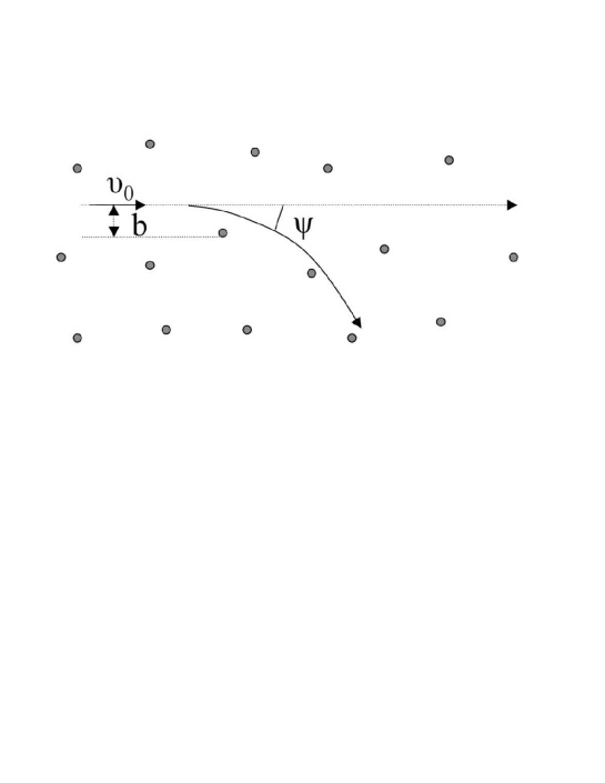
Figure 1: Deflection of a test particle (star) moving in a homogeneous sea of other particles.

Due to Chandrasekhar’s calculation of the relaxation time, the basic paradigm for galaxies is a collisionless stellar system in which the collisionless Boltzmann equation applies (subsection 2.3). However, the true nature of relaxation depends also somewhat on what region of the galaxy we consider as well as on the properties of the system’s stellar orbits. For example, the above analysis is not precise at the centers of galaxies, especially when the latter are occupied by large central mass concentrations. Furthermore, if a system has a large degree of stochasticity, i.e., many orbits with Lyapunov times smaller or equal to the Hubble time, then the two-body relaxation time for such a system is drastically reduced, perhaps by more than three orders of magnitude (Gurzandyan and Savvidy 1986, Pfenniger 1986). This is because an initially small deflection, caused by a two-body encounter, is amplified by the mechanism of exponential deviations of nearby orbits due to positive Lyapunov exponents. This may have affected systems that are ‘granular’, for example galaxies containing a high percentage of globular clusters (Udry and Pfenniger 1988). The extent to which such phenomena appear in real galaxies is not yet fully known.

2.2 Distribution function

The most basic quantity in stellar systems is the fine-grained distribution function:

$$f(\mathbf{x},\mathbf{v},t)=\lim_{d^{6}\mu\rightarrow 0}\frac{dm(\mathbf{x},\mathbf{v},t)}{d^{3}\mathbf{x}d^{3}\mathbf{v}}$$ (4)

yielding the mass $dm(\mathbf{x},\mathbf{v},t)$ contained at time $t$ within an infinitesimal phase-space volume $d^{6}\mu=d^{3}\mathbf{x}d^{3}\mathbf{v}$ centered around any point $(\mathbf{x},\mathbf{v})$ of the 6D phase space of stellar motions (called the $\mu-$space in statistical mechanics). In the N-Body approximation the mass $dm(\mathbf{x},\mathbf{v},t)$ can be considered proportional to the number of particles, i.e., stars or fluid elements of the dark matter, within the volume $d^{3}\mathbf{x}d^{3}\mathbf{v}$. Furthermore, it is often convenient to introduce a coarse-grained distribution function

$$F(\mathbf{x},\mathbf{v},t)={1\over\Delta^{3}\mathbf{x}\Delta^{3}\mathbf{v}}\int_{\Delta^{3}\mathbf{x}\Delta^{3}\mathbf{v}}f(\mathbf{x},\mathbf{v},t)d^{3}\mathbf{x}d^{3}\mathbf{v}$$ (5)

which gives the average of the fine-grained distribution function $f$ in small, but not infinitesimal volume elements $\Delta^{3}\mathbf{x}\Delta^{3}\mathbf{v}$ around the phase space points $(\mathbf{x},\mathbf{v})$. Contrary to the fine-grained distribution $f$, the value of the coarse-grained distribution $F$ depends on the particular choice of partitioning of the phase-space by which the volume elements $\Delta^{3}\mathbf{x}\Delta^{3}\mathbf{v}$ are defined. This fact has some interesting implications in the modelling process of a galaxy, discussed in section 3 below.

The distribution function can be used to derive several other useful quantities. For example, the spatial mass density $\rho(\mathbf{x},t)$ of the system is given by the integral of the d.f. $f$ over velocities, e.g. (in Cartesian coordinates)

$$\rho(\mathbf{x},t)=\int_{-\infty}^{\infty}\int_{-\infty}^{\infty}\int_{-\infty}^{\infty}f(\mathbf{x},\mathbf{v},t)dv_{x}dv_{y}dv_{z}$$ (6)

The latter quantity, $\rho(\mathbf{x},t)$, can be used in turn to calculate the gravitational potential $\Phi(\mathbf{x},t)$ via Poisson’s equation:

$$\nabla^{2}\Phi(\mathbf{x},t)=4\pi G\rho(\mathbf{x},t)~{}~{}~{}.$$ (7)

The orbits of stars are given by the Hamiltonian

$$H(\mathbf{x},\mathbf{p},t)\equiv{\mathbf{p}^{2}\over 2}+\Phi(\mathbf{x},t)$$ (8)

setting, for simplicity, $\mathbf{p}=\mathbf{v}$ in Cartesian coordinates and the average stellar mass equal to unity. We often consider galaxies in steady state equilibrium (subsection 2.3), in which case we drop the explicit dependence of $f$ on the time $t$:

$$H(\mathbf{x},\mathbf{p})\equiv{\mathbf{p}^{2}\over 2}+\Phi(\mathbf{x})~{}~{}~{}.$$ (9)

Assuming a nearly constant mass-to-light ratio, the observable photometric or kinematic profiles of a galaxy can be deduced from various moments of $f$. For example, if the axis $x$ is identified to the direction of the line of sight, the surface density at any point $\mathbf{R}\equiv(y,z)$ of the plane of projection normal to $x$ is given by:

$$\Sigma(\mathbf{R})=\int_{-\infty}^{\infty}\rho(x,\mathbf{R})dx$$ (10)

with $\rho$ given by Eq.(6). The quantity $\Sigma(\mathbf{R})$ can be compared to observed surface brightness profiles. On the other hand, the line-of-sight velocity distribution at a particular point $\mathbf{R}$ of the same plane of projection is given by

$$LOSVD(\mathbf{R},v_{x})={1\over\Sigma(R)}\int_{-\infty}^{\infty}\int_{-\infty}^{\infty}\int_{-\infty}^{\infty}dxdv_{y}dv_{z}f(x,\mathbf{R},v_{x},v_{y},v_{z})$$ (11)

and the latter quantity can be compared to the profiles of spectral lines determined also observationally. Via the line-of-sight velocity distributions we can determine mean velocity profiles,

$$\mu(\mathbf{R})=\int_{-\infty}^{\infty}v_{x}LOSVD(\mathbf{R},v_{x})dv_{x}$$ (12)

and velocity dispersion profiles

$$\sigma^{2}(\mathbf{R})=\int_{-\infty}^{\infty}(v_{x}-\mu(\mathbf{R}))^{2}LOSVD(\mathbf{R},v_{x})dv_{x}~{}~{}.$$ (13)

Also related to observations is the concept of velocity ellipsoid. This is an ellipsoid in velocity space assigned to every point $\mathbf{x}$ of ordinary space. Fixing an orthogonal coordinate system, say, Cartesian axes $x_{1}=x,x_{2}=y,x_{3}=z$, we calculate the second moments

$$\sigma_{ij}^{2}(\mathbf{x})={1\over\rho(\mathbf{x})}\int_{-\infty}^{\infty}(v_{i}-V_{i})(v_{j}-V_{j})f(\mathbf{x},\mathbf{v})d^{3}\mathbf{v}$$ (14)

where the indices $i,j$ run the values $1,2$, or $3$, $V_{i}$ is the mean velocity in the i-th direction at the point $\mathbf{x}$ and the integral denotes a triple integral with respect to the velocities. The $3\times 3$ matrix $\mathbf{\sigma}$, with elements $\sigma_{ij}$, is symmetric, thus it has three real eigenvalues, say $\sigma_{1}$, $\sigma_{2}$, and $\sigma_{3}$ and unit eigenvectors $\mathbf{e}_{\sigma,k}$, $k=1,2,3$. The velocity ellipsoid is defined by the equation

$$\sum_{k=1}^{3}{(\mathbf{v}\cdot\mathbf{e}_{\sigma,k})^{2}\over\sigma_{k}^{2}}=1~{}~{}.$$ (15)

The shape of the velocity ellipsoid at a point $\mathbf{x}$ gives the dispersion of the distribution of velocities in different local directions of motion. In particular, a system is called isotropic at the point $\mathbf{x}$ if the velocity ellipsoid at $\mathbf{x}$ is a sphere, otherwise it is called anisotropic. In the case of anisotropic systems, we further distinguish systems with two or three unequal axes of the velocity ellipsoid. This distinction is important, because it allows one to link the kinematic observations available for a particular system to dynamical features of the same system. For example, the observation that the velocity ellipsoid in the Solar neighborhood has three unequal axis led to the discovery that the stellar orbits in the Solar neighborhood are subject to a ‘third integral’ (Contopoulos 1960), besides the energy and angular momentum integrals.

2.3 Stellar dynamical equilibria - Old and new versions of Jeans’ Theorem

The basic equation governing the time evolution of the distribution function $f$ in collisionless stellar systems is Liouville’s equation implemented in the $\mu-$space of motion of the Hamiltonian (8), otherwise called Boltzmann’s equation (or Vlasov’s equation in plasma physics):

$${df\over dt}={\partial f\over\partial t}+\mathbf{p}{\partial f\over\partial\mathbf{x}}-{\partial\Phi\over\partial\mathbf{x}}{\partial f\over\partial\mathbf{p}}=0$$ (16)

where we have adopted the notation $\mathbf{p}\equiv\mathbf{v}$ for canonical momenta, i.e., consider stellar masses equal to unity. Eq.(16) states that the mass contained within any infinitesimal volume $d^{6}\mu$ that travels in phase space along the orbits corresponding to the potential $\Phi$ (determined by Eq.(7)) is preserved. Furthermore, the measure of the volume $d^{6}\mu$ is also preserved (Liouville’s theorem). Now, the morphological regularity and the commonly observed characteristics of most galaxies suggest that the majority of these systems are close to a state of statistical equilibrium. Thus, we often look for steady-state solutions of Eq.(16) that do not have an explicit dependence of $f$ on time. Setting $\partial f/\partial t=0$ in Eq.(16) yields

$$\mathbf{p}{\partial f\over\partial\mathbf{x}}-{\partial\Phi\over\partial\mathbf{x}}{\partial f\over\partial\mathbf{p}}=\{f,H\}=0$$ (17)

where $\{\cdot,\cdot\}$ denotes the Poisson bracket operator.

Despite its formal simplicity, the physical content of Eq.(17) is remarkable. Consider a fixed phase volume $d^{6}\mu$ centered at some phase space point $(\mathbf{x},\mathbf{p})$ of a galaxy in steady-state equilibrium. The stars follow orbits determined by the Hamiltonian (9). The orbits remain smooth in the course of time, because there are no short range stochastic force terms affecting the stars, similar, for example, to collisions in a perfect gas. Nevertheless, a detailed equilibrium is established in the phase space, i.e., if Eq.(17) is valid the number of stars leaving the volume $d^{6}\mu$ at any moment $t$ must be equal to the number of stars entering the same volume. Furthermore, the gravitational potential determining the orbits is given by Eq.(7), which involves also the positions of the stars. This means that the motions of the stars are combined in such a way so as to reproduce the same macroscopic distribution of matter continually in time. For this reason, galactic equilibria are called self-consistent, i.e., supported solely by the orbits of stars within the system. It is a great theoretical challenge to understand the processes by which nature forms such remarkable systems.

Consider a system in steady-state equilibrium and suppose that the mathematical form of the function $f(\mathbf{x},\mathbf{p})$ was given. Then, according to Eq.(17), the function $f$ constitutes an integral of the motion in involution with the Hamiltonian. If, on the other hand, we know by independent means a complete set of functionally independent integrals of motion $I_{1},I_{2},...$ under the Hamiltonian flow of $H$, it follows that $f$ is necessarily a composite function of the phase space canonical variables $(\mathbf{x},\mathbf{p})$ through one or more of the integral functions $I_{1},I_{2},...$. That is

$$f(\mathbf{x},\mathbf{p})\equiv f(I_{1}(\mathbf{x},\mathbf{p}),I_{2}(\mathbf{x},\mathbf{p}),\ldots)~{}~{}~{}.$$ (18)

The last equation is known as Jeans’ theorem of stellar dynamics (Jeans 1915).

Although fundamental in theory, Jeans’ theorem, in the above general form, is of limited usefulness, because it specifies neither a) which integrals out of the set $I_{1},I_{2},...$ should actually appear as arguments in the distribution function of a specific system, nor b) the explicit form of the dependence of $f$ on these integrals. Regarding point (a), a ‘strong’ Jeans theorem proved by Lynden-Bell (1962a) asserts that only isolating integrals can be arguments of the function $f$. An integral $I_{i}$ is called isolating if the constant value condition $I_{i}(\mathbf{x}(t),\mathbf{p}(t))=c_{i}$ defines a manifold in phase space of dimension lower than the phase space dimension (equal to six for three dimensional systems). If we have a set of $M$ isolating integrals $I_{1},I_{2},...I_{M}$, any orbit $(\mathbf{x}(t),\mathbf{p}(t))$ is restricted on a sub-manifold of phase space which is the intersection of all the manifolds defined by the constant value conditions $I_{i}(\mathbf{x}(t),\mathbf{p}(t))=c_{i},i=1,2,...,M$.

A case of particular interest is when the Hamiltonian of motion $H$ is integrable in the Arnold-Liouville sense. In three degrees of freedom systems this means that there are three functionally independent integrals ($H$ itself can be taken as one of them) which are mutually in involution, namely

$$\{I_{i},I_{j}\}=\sum_{k=1}^{3}{\partial I_{i}\over\partial x_{k}}{\partial I_{j}\over\partial p_{k}}-{\partial I_{i}\over\partial p_{k}}{\partial I_{j}\over\partial x_{k}}=0~{}~{}~{}.$$ (19)

In that case, the Arnold-Liouville theorem (see e.g. Arnold 1978 or Giorgilli 2002) asserts that if the manifolds defined by the constant value conditions $I_{i}(\mathbf{x}(t),\mathbf{p}(t))=c_{i},i=1,2,3$ are compact, then they are topologically equivalent to 3-tori. The integrals $I_{i},i=1,2,3$ are isolating and the strong Jeans theorem takes the following form: if the Hamiltonian of a collisionless stellar system in steady-state equilibrium is Arnold-Liouville integrable, the fine-grained distribution function $f$ has constant value at all the points $(\mathbf{x},\mathbf{p})$ of an invariant torus of the system.

We examine below some simple examples of application of the strong Jeans theorem in stellar dynamics.

Spherical systems

A spherical system in equilibrium is the simplest model of a galactic system. This model is not very realistic, but it serves a) to introduce some basic concepts, and b) as a starting point for the analysis of more realistic systems. In spherical coordinates, the distribution function depends on $r$ and on the three velocity components $v_{r}=\dot{r}$, $v_{\theta}=r\dot{\theta}$, $v_{\phi}=r\sin\theta\dot{\phi}$, namely $f\equiv f(r,v_{r},v_{\theta},v_{\phi})$. The mass density depends only on $r,$ $\rho\equiv\rho(r)$. The orbits are determined by a spherical potential $\Phi(r)$, given by the solution of Eq.(7):

$$\Phi(r)=-\frac{GM(r)}{r}-\int_{r}^{\infty}{Gdm(r^{\prime})\over r^{\prime}}=-{G\over r}\int_{0}^{r}4\pi r^{\prime 2}\rho(r^{\prime})dr^{\prime}-G\int_{r}^{\infty}4\pi r^{\prime}\rho(r^{\prime})dr^{\prime}$$ (20)

The orbits obey three isolating integrals of motion in involution, namely the energy $E=H$, and the components of the angular momentum $p_{\theta}=r^{2}\dot{\theta}$ and $p_{\phi}=r^{2}sin^{2}\theta\dot{\phi}$. The angular momentum vector $\mathbf{L}=\mathbf{r}\times\mathbf{v}$ is constant and an orbit is restricted on the plane normal to $\mathbf{L}$. The modulus $L=|\mathbf{L}|$ is an integral in involution with $p_{\phi}$, and the triplet $(E,L,p_{\phi})$ is the usual choice of integrals in the study of spherical systems.

According to the strong Jeans’ theorem, the general form of the distribution function $f(r,v_{r},v_{\theta},v_{\phi})$ in equilibrium can only be a composite function:

$$f\equiv f(E(r,v_{r},v_{\theta},v_{\phi}),L(r,v_{r},v_{\theta},v_{\phi}),p_{\phi}(r,v_{r},v_{\theta},v_{\phi}))$$ (21)

Further restrictions in the form of $f$ can be imposed on the basis of the kinematical properties of the system under study. For example, if the system has no preferential kinematical axis (e.g. an axis of rotation), the integral $p_{\phi}$ cannot appear as an argument in $f$. This implies that there is equal probability to find a star moving in a plane of any possible orientation with respect to the galactic frame of reference. This is applicable, e.g., to the spherical limit of giant elliptical galaxies, since there is evidence that the these galaxies are not rotationally supported against gravity (e.g. Bertola and Capaccioli 1975, Illingworth 1977, Davies et al. 1983) but they are ‘hot systems’ with small or no rotation, in which gravity is balanced by the distribution of velocities in random directions (e.g. Binney 1976, 1978). In the spherical limit, we use distribution functions of the form $f(E)$ or $f(E,L)$. If $f\equiv f(E)$ the galaxy is called isotropic. The expression for the orbital energy $E=v_{r}^{2}/2+v_{\theta}^{2}/2+v_{\phi}^{2}/2+\Phi(r)$ yields a symmetric dependence of $f$ on either of the three velocity components. This implies equal axes of the velocity ellipsoid $\sigma_{r}^{2}=\sigma_{\theta}^{2}=\sigma_{\phi}^{2}$. On the other hand, if $f\equiv f(E,L)$ the system is called anisotropic. The appearance of $L=r\sqrt{v_{\theta}^{2}+v_{\phi}^{2}}$ in $f$ breaks the symmetry of the functional dependence of $f$ on $v_{r}$ and $v_{\theta}$ (or $v_{\phi}$). The velocity ellipsoid has two equal axes $\sigma_{r}^{2}\neq\sigma_{\theta}^{2}=\sigma_{\phi}^{2}$. Since every orbit is confined to a plane, we consider the total velocity in the transverse direction of motion $v_{t}^{2}=v_{\theta}^{2}+v_{\phi}^{2}$ and define the anisotropy parameter $\beta(r)$ (Binney and Tremaine 1987, p.204):

$$\beta(r)=1-{\sigma_{r}^{2}(r)\over 2\sigma_{t}^{2}(r)}$$ (22)

with

$$\sigma_{r}^{2}(r)={1\over\rho(r)}\int_{0}^{\sqrt{-2\Phi(r)}}\int_{0}^{\sqrt{-2\Phi(r)-v_{r}^{2}}}fv_{r}^{2}v_{t}dv_{r}dv_{t}$$

and

$$\sigma_{t}^{2}(r)={1\over\rho(r)}\int_{0}^{\sqrt{-2\Phi(r)}}\int_{0}^{\sqrt{-2\Phi(r)-v_{r}^{2}}}fv_{t}^{3}dv_{r}dv_{t}~{}~{}~{}.$$

The limits of integration in the above equations are imposed by the consideration of only bound orbits ($E<0$). The parameter $\beta$ is a function only of $r$. In practice we find that realistic systems are nearly isotropic in their central parts, $\beta(r)\rightarrow 0$ as $r\rightarrow 0$, and radially anisotropic in their outer parts, i.e., $\beta(r)\rightarrow 1$ for $r$ large. This means that there is a predominance of radial orbits in the outer part of the galaxy, i.e., orbits with a large difference between the apocentric and pericentric distances. This phenomenon is linked to the relaxation process of galaxies (section 3). In particular, this is the expected final behavior of systems subject to a phase of ‘collapse’ (Eggen et al. 1962), and this behavior is confirmed by N-Body experiments of violent relaxation (e.g. Aguilar and Merritt 1990, Voglis 1994a).

Axisymmetric systems and the ‘third integral’ of motion

The Hamiltonian of motion in an axisymmetric galaxy can be written in cylindrical canonical variables $(R,\phi,z,p_{R},p_{\phi},p_{z})$:

$$H\equiv{p_{R}^{2}\over 2}+{p_{\phi}^{2}\over 2R^{2}}+{p_{z}^{2}\over 2}+\Phi(R,z)$$ (23)

where $z$ is the axis of symmetry, and $p_{R}=\dot{R}$, $p_{\phi}=R^{2}\dot{\phi}$, $p_{z}=\dot{z}$. Since the azimuthal angle $\phi$ is ignorable, the canonical momentum $p_{\phi}$ is a second integral of motion, besides the energy $E=H$. This can be identified to the z-projection of the angular momentum vector $p_{\phi}=L_{z}$. The study of orbits can be simplified by considering only the motion on the meridional plane $(R,z)$

$$\ddot{R}=-{\partial\Phi\over\partial R}+{L_{z}^{2}\over R^{3}},~{}~{}~{}~{}\ddot{z}=-{\partial\Phi\over\partial z}~{}~{}.$$ (24)

The form of these equations implies that Eq.(23) can be viewed as a two degrees of freedom Hamiltonian, where $p_{\phi}$, replaced by $L_{z}$, is considered as a parameter. The angular motion is readily found via $\dot{\phi}=L_{z}/R^{2}$. The orbits on the equatorial plane are defined by a central potential $\Phi(R,0)$ (provided that the system is symmetric with respect to the equatorial plane, i.e., the function $\Phi(R,z)$ is even with respect to $z$).

If we consider circular orbits in the equatorial plane for a particular value of $L_{z}$, the circular radius is given by the root of the equation:

$$-{\partial\Phi(R_{c},0)\over\partial R}+{L_{z}^{2}\over R_{c}^{3}}=0$$ (25)

The circular orbit appears as a equilibrium point on the meridional plane, at $R=R_{c},\dot{R}=0$. If we expand the Hamiltonian with respect to this point we get (ignoring a constant term $L_{z}^{2}/2R_{c}^{2}$):

$$H={1\over 2}\big{(}p_{Y}^{2}+p_{z}^{2}+\omega_{Y}^{2}Y^{2}+\omega_{z}^{2}z^{2}\big{)}+\sum_{k=3}^{\infty}H^{(k)}(Y,z;L_{z})$$ (26)

where $Y=R-R_{c}$, $\omega_{Y}^{2}=\dfrac{\partial^{2}\Phi(R_{c},0)}{\partial^{2}R}+\dfrac{3L_{z}^{2}}{R_{c}^{4}}$, $\omega_{z}^{2}=\dfrac{\partial^{2}\Phi(R_{c},0)}{\partial^{2}z}$, and the functions $H^{(k)}(Y,z;L_{z})$ are polynomials of degree $k$ in the variables $Y,z$, depending also on $L_{z}$ as a parameter.

The Hamiltonian (26) has a particular place in the history of both galactic dynamics and dynamical systems theory because a) it is the first Hamiltonian for which a ‘third integral’ of motion was calculated (Contopoulos 1960), and b) its third order truncation yields the Hénon - Heiles (1964) Hamiltonian that has served as a prototype of many studies in nonlinear Hamiltonian dynamical systems.

Special forms of the third integral, e.g. quadratic in the velocities, were considered by various authors (see references in Ogorodnikov 1965). On the other hand, Contopoulos (1960) explored the question of whether a third integral of motion $I$, besides $H$ and $L_{z}$ can be constructed algorithmically for the Hamiltonian (26). The existence of $I$ implies that all the orbits are regular (no chaos is present). Furthermore, according to Jeans’ theorem’s the integral can possibly appear as an argument in the distribution function. Recalling arguments similar to the spherical case, we then find that if $f$ depends on $I$ the velocity ellipsoid at any point of ordinary space has unequal axes $\sigma_{R}\neq\sigma_{z}$, while if $f$ does not depend on $I$ the dispersions are equal $\sigma_{R}=\sigma_{z}$. The observational data in our own Galaxy, in the Solar neighborhood, favored the former case to be true.

Contopoulos (1960) combined two earlier methods of Whittaker (1916) and Cherry (1924a,b) in order to show that, in the so-called non-resonant case, when the frequencies $\omega_{Y}$, $\omega_{z}$ are incommensurable, an integral can be formally constructed in the form of a polynomial series in the canonical variables, by an algorithm which is significantly simpler than the use of canonical transformations as in the Birkhoff - von Zeipel method (Birkhoff 1927), widely used in Celestial Mechanics. Given that such formal series are, in general, not convergent (Siegel 1941), the above series does not represent a real third integral of the system. However, we shall see below that the series has an asymptotic behavior. Namely, if we define a remainder $R^{(n)}$ for the series at the n-th order of truncation, the remainder initially decreases as $n$ increases, giving the impression that the series is convergent. However, after an optimal order $n_{opt}$ the remainder becomes an increasing function of $n$ (Fig.2), implying divergence of the series. If we truncate the integral series at the order $n_{opt}$, we obtain a function $I=I^{(2)}+I^{(3)}+...+I^{(n_{opt})}$ which is an approximate integral of motion, in the sense that the time variations $dI/dt$ are quite small, of order $R^{(n_{opt})}$. The apparent improvement of the accuracy of the integral as $n$ increases (below $n_{opt}$) was checked by a computer program that calculated the series (Contopoulos and Moutsoulas 1965). This was confirmed later by Gustavson (1966) with a calculation of the Birkhoff series in the Hénon - Heiles Hamiltonian.

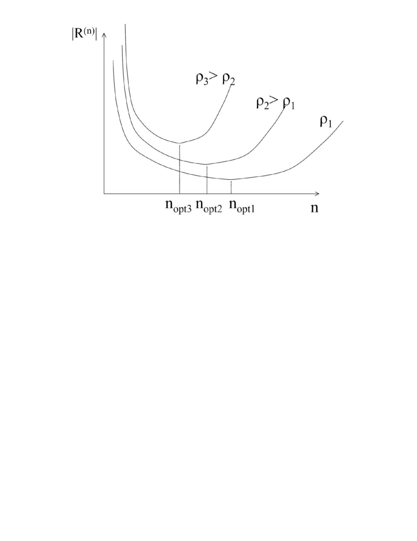
Figure 2: Asymptotic behavior of the ‘third integral’. The size of the remainder $|R^{(n)}|$ of the integral series as a function of the order of truncation $n$ for three different effective distances from the equilibrium point.

While in the non-resonant case the calculation of the third integral by the direct method of Contopoulos is simpler than by the Birkhoff normal form, the situation is reversed in the case of resonant integrals, i.e., when the frequencies satisfy a commensurability relation $m_{1}\omega_{Y}+m_{2}\omega_{z}=0$, with $m_{1},m_{2}$ integers. A direct method to construct a resonant integral without use of a normal form was given by Contopoulos (1963) and exploited in the case of particular resonances by Contopoulos and Moutsoulas (1965). However, this method involves a ‘back and forth’ algorithm between successive orders of truncation, which is an essential complication. The discrete analog of the direct method for symplectic mappings was given by Bazzani and Marmi (1991), in the non-resonant case, and by Efthymiopoulos (2005) in the resonant case. However, all these direct methods are currently superseded by the use of the Birkhoff method via Lie canonical transformations (Hori 1966, Deprit 1969, Giorgilli and Galgani 1978, Verhulst 1979), which is the simplest method to implement in the computer (e.g. Giorgilli 1979).

The Lie method of construction of a third integral was implemented in axisymmetric galaxies by Gerhard and Saha (1991). These authors studied various constructive methods of the canonical perturbation theory. A particular method is to express the Hamiltonian in the action-angle variables of the spherical part of the potential, since analytical expressions yielding the action-angle variables in terms of the usual canonical variables are explicitly known in that case. The Lie method can then be used in order to construct a formal third integral, besides the energy and $L_{z}$. The so-obtained expressions represented a well-preserved integral if the system’s axial ratio was greater than 0.5. Further models of this type were given by Dehnen and Gerhard (1993), starting from the spherical isochrone model (subsection 3.4) to represent the unperturbed system. On the other hand, Matthias and Gerhard (1999) tested whether the boxy elliptical galaxy NGC 1600 is better fitted by a two-integral or three-integral model. They found that three-integral models better reproduce the available kinematic data for the galaxy. This conclusion was confirmed in subsequent studies (e.g. Gebhardt et al. 2000, 2001, Cappellari et al. 2002, Verolme et al. 2002, Dejonghe and Bruyne 2003, sect. 4 and references therein). We will return below to the question of the choice between two-integral or three-integral axisymmetric models, when discussing relevant results from N-Body simulations.

Besides the harmonic oscillators, or the spherical model, there are other integrable axisymmetric models that can serve as starting models for the construction of formal third integrals. For example, Petrou (1983) constructed a third integral starting from an axisymmetric model of the form $\Phi(r,\theta)=\Phi_{0}(r)+\Phi_{1}(\theta)/r^{2}$ (in polar coordinates) which is known to be integrable (e.g. Goldstein 1980, p.457). Another possible choice is an axisymmetric Stäckel potential (Stiavelli and Bertin 1987, Dejonghe et al. 1996). Other models based on local Stäckel fits are reviewed in Dejonghe and Bruyne (2003).

When the potential has a central cusp, a convenient method to calculate third integrals is the semi-analytical (or semi-numerical) method. Essentially, this means to start with a plausible model in which action - angle variables are explicitly constructed, and then to introduce canonical transformations to new action - angle variables with generating functions specified through a numerical criterion. This criterion can be based on either the ‘theoretical’ Hamiltonian flow (found by the normal form) fitting the true Hamiltonian flow of the system, or the theoretical tori, viewed as geometrical objects, fitting the real tori of the system. Such fitting methods were introduced in galactic dynamics by Ratcliff et al. (1984), McGill and Binney (1990) and Kent and de Zeeuw (1991).

(Non-)convergence properties of the ‘third integral’. The theory of Nekhoroshev

The optimal order of truncation $n_{opt}$ of the third integral series, as well as the size of the optimal remainder $R^{(opt)}$ are questions that can be examined in the framework of the theory of Nekhoroshev (Nekhoroshev 1977, Benettin et al. 1985, Lochak 1992, Pöshel 1993), implemented, in particular, in the case of elliptic equilibria (Giorgilli 1988, Fassò et al. 1998, Guzzo et al. 1998, Niederman 1998). This theory states that as the parameter $\epsilon$ that quantifies the perturbation of the system from an integrable system decreases, the size of the optimal remainder becomes exponentially small in $1/\epsilon$, that is:

$$R_{opt}=O\left(\exp\left(-{1\over\epsilon^{p}}\right)\right)$$ (27)

where the exponent $p$ depends on the number of degrees of freedom of the system under study. Conversely, approximate integrals of the type of the ‘third integral’ retain almost constant values for times exponentially long in $1/\epsilon$, that is, $T_{Nek}=O(\exp(1/\epsilon^{p}))$. In galactic Hamiltonians such as (26), the effective perturbation $\epsilon$ is identified to the average distance $\rho$ of an orbit from the elliptic equilibrium. Thus, without being able to prove the existence of an exact third integral for the orbits $R(t),z(t)$ on the meridional plane, we can assert that, even if such orbits are chaotic, an orbit will behave effectively like regular for a time exponentially long in $1/\rho$, where $\rho$ is the distance of the orbit from the equilibrium $R=R_{c},z=0$.

A heuristic derivation of the formula $R_{opt}=O\big{(}\exp(-1/\rho)\big{)}$, based on the use of integrals calculated by the direct method, can be given following a theorem by Giorgilli (1988). We make the derivation in action - angle variables $(J,\phi)$. We set $Y=\sqrt{2J_{1}}\sin\phi_{1}$, $p_{Y}=\sqrt{2J_{1}}\cos\phi_{1}$, $z=\sqrt{2J_{2}}\sin\phi_{2}$, $p_{z}=\sqrt{2J_{2}}\cos\phi_{2}$, and $\omega_{1}\equiv\omega_{Y}$, $\omega_{2}\equiv\omega_{z}$. The Hamiltonian (26) takes the form

$$H=\omega_{1}J_{1}+\omega_{2}J_{2}+\sum_{k=3}^{\infty}H^{(k)}(J_{1},J_{2},\phi_{1},\phi_{2})$$ (28)

where the functions $H^{(k)}$ are of degree $k/2$ in the actions and contain trigonometric terms of the form $e^{i(k_{1}\phi_{1}+k_{2}\phi_{2})}$ with $k_{1},k_{2}$ integers, $|k_{1}|+|k_{2}|\leq k$ and of the same parity as $k$. We look for a third integral as a series yielding a correction to the action $J_{1}$, or $J_{2}$ (each of the actions is an exact integral in the harmonic oscillator limit of Eq.(26)). We thus set

$$I=J_{1}+\sum_{k=3}^{\infty}I^{(k)}(J_{1},J_{2},\phi_{1},\phi_{2})~{}~{},$$

the functions $I^{(k)}$ satisfying the same properties as the functions $H^{(k)}$ (we set $I^{(2)}=J_{1}$). The integral is calculated by splitting the integral condition $\{I,H\}=0$ to terms of equal order. This yields the relation

$$\{I^{(k)},H^{(2)}\}=-\sum_{s=2}^{k-1}\{I^{(s)},H^{(k+2-s)}\}$$ (29)

with $H^{(2)}=\omega_{1}J_{1}+\omega_{2}J_{2}$. Eq.(29) can be solved recursively to yield $I^{(k)}$ in the k-th step from the terms $I^{(s)}$, $s=2,...,k-1$ determined in the previous steps. If we express the terms $I^{(s)}$ in sums of Fourier terms of the form $J_{1}^{s_{1}\over 2}J_{2}^{s_{2}\over 2}e^{i(k_{1}\phi_{1}+k_{2}\phi_{2})}$, we readily see that the algebraic nature of the direct scheme (29) is quite similar to that of the Birkhoff-von Zeipel normal form scheme: Each Fourier term is an eigenfunction of the linear differential operator $\{\cdot,H^{(2)}\}$ with eigenvalue equal to $-i(k_{1}\omega_{1}+k_{2}\omega_{2})$, that is

$$\{J^{s\over 2}e^{ik\cdot\phi},H^{(2)}\}=-i(k\cdot\omega)J^{s\over 2}e^{ik\cdot\phi}$$

where we use the abbreviations $J^{s\over 2}\equiv J_{1}^{s_{1}\over 2}J_{2}^{s_{2}\over 2}$, $k\equiv(k_{1},k_{2})$, $\omega\equiv(\omega_{1},\omega_{2})$. This implies that the solution of Eq.(29) for $I^{(k)}$ yields precisely a sum of the same Fourier terms as in the r.h.s. of the same equation, each term being divided by the divisor $k\cdot\omega$. The presence of divisors is important because, for generic incommensurable frequency vectors $\omega$ there are integer vectors $k$ that can be found, which render the product $k\cdot\omega$ a small divisor. For example, from number theory it is known (e.g. Berry 1978) that most irrationals satisfy diophantine conditions of the form

$$|k\cdot\omega|\geq{\gamma\over|k|^{\tau}}$$ (30)

with $\gamma$ an $O(1)$ constant and $\tau$, the diophantine exponent, depending on the number of degrees of freedom ($\tau\geq n-1$). This means that, as $|k|$ increases, the minimum size of divisors appearing in the recurrent solution of Eq.(29) decreases, i.e., the divisors become smaller and smaller. Furthermore, as one repeatedly implements the recurrence relation, such small divisors accumulate in the form of products in the denominators of the various integral terms. That is, there are Fourier terms $f^{(k)}$ in $I^{(k)}$ with an accumulation of divisors yielding a size

$$||f^{(k)}||\sim{F^{(k)}\over a_{3}a_{4}...a_{k}}$$ (31)

with divisors $a_{s},s=3,4,\ldots,k$ satisfying $a_{s}\sim 1/s^{\tau}$ according to Eq.(30). The numerator $F^{(k)}$ in Eq.(31) can be estimated by the remark that, for any term $I^{(s)}$, the Poisson bracket in the r.h.s. of Eq.(29) means to take the derivatives $\partial I^{(s)}/\partial J$, or $\partial I^{(s)}/\partial\phi$, which both cause the appearance of a factor $O(s)$ in front of the corresponding Fourier terms of $I^{(s)}$. Hence, the repeated action of Poisson brackets, up to order $k$ creates a factor $F^{(k)}\sim O(3)O(4)...O(k)\sim k!$ in the numerator of the Fourier terms of $I^{(k)}$ (see Efthymiopoulos et al. 2004 for a more detailed analysis). Putting these remarks together, the size of Fourier terms (31) can be estimated as $||f^{(k)}||\sim k!^{\tau+1}$. If we now consider an orbit of effective distance $\rho$ from the equilibrium, we have $J^{s/2}\sim\rho^{s}$ for this orbit, so that the value of the remainder of the formal series at the k-th order of truncation can be estimated as:

$$R^{(k)}\sim k!^{\tau+1}\rho^{k}$$ (32)

The estimate (32) contains the essential result regarding the asymptotic character of formal series: using Stirling’s formula $k!\sim(k/e)^{k}$, for large k, we have $R^{(k)}\sim(k^{\tau+1}\rho/e^{\tau+1})^{k}$. We then want to check whether the remainder decreases or increases as the order $k$ of calculation of the formal integral increases. We see immediately that as long as $k<<e/\rho^{1/(\tau+1)}$, the remainder decreases with $k$, while if $k>>e/\rho^{1/(\tau+1)}$ the remainder increases with $k$. Thus the optimal order is at an order $n_{opt}$ were the remainder is minimum, which can be estimated as $n_{opt}\sim e/\rho^{1/(\tau+1)}$. Inserting this in Eq.(32) we find the value of the remainder at the optimal order of truncation $R_{opt}\sim\exp(-n_{opt})\sim\exp(-1/\rho^{(1/(\tau+1)})$, which leads to Nekhoroshev’s formula of exponentially small time variations of the truncated integral $I=I^{(2)}+I^{(3)}+...+I^{(n_{opt})}$.

In generic nearly-integrable Hamiltonian systems of the form $H(J,\phi)=H_{0}(J)+\epsilon H_{1}(J,\phi)$ the Nekhoroshev theory is much more complicated than in the simple case of elliptic equilibria. The main complication is that the frequencies $\omega(J)=\partial H/\partial J$ depend on the actions, a fact that renders necessary the separate treatment of several non-resonant or resonant domains that coexist in the space of actions. This treatment is the so-called geometric part of Nekhoroshev theorem (see Morbidelli and Guzzo 1997 for an instructive introduction and Giorgilli 2002 for a rigorous but still pedagogical proof). On the other hand, the analytic part of the theorem is treated more easily if we avoid dealing with repeated Poisson brackets, as above, acting on the series terms of successive orders of normalization. This is done by setting from the start a number of assumptions regarding the analyticity properties of the Hamiltonian under consideration in a complexified space of actions and angles and by using various forms of Cauchy theorem for analytic functions. This simplifies considerably the proof of the analytical part of the theorem.

Nevertheless, it seems that when one wants to find realistic estimates as regards the optimal order of truncation and the optimal value of the remainder, one has to rely on the classical methods of analysis of series convergence. The first systematic exploitation of these questions, referring to the method of Birkhoff series, was made by Servizi et al. (1983), who calculated ‘pseudoradii of convergence’ for the Birkhoff normal form in symplectic mappings representing the Poincaré surface of section of 2D Hamiltonian systems. Kaluza and Robnik (1992) found that there was no indication of divergence of the formal series below the order $n=15$ in the Hénon - Heiles model. A particular application in the problem of stability of the Trojan asteroids (Giorgilli and Skokos 1997) showed that the optimal order of truncation of the integrals in this case is beyond $n=32$ (in some cases we find $n_{opt}>60$, Efthymiopoulos and Sándor 2005). But a precise treatment of the problem was made only very recently (Contopoulos et al. 2003, Efthymiopoulos et al. 2004). In these works scaling formulae are given yielding the optimal order of truncation as a function of the distance from the elliptic equilibrium and of the number of degrees of freedom. These formulae are derived theoretically and verified by computer algebraic calculations. A recent application in the case of galactic potentials was given by Belmonte et al. (2006).

The estimate $n_{opt}\sim e/\rho^{1/(\tau+1)}$ implies that the optimal order of truncation is smaller, and the value of the optimal remainder is larger, for larger $\rho$. This behavior is shown schematically in Fig.2. On the other hand, when $\rho$ surpasses a threshold value $\rho_{c}$, at which $n_{opt}$ approaches the lowest possible value $n_{opt}=3$, there is no more meaning in calculating a third integral $I$, since the series will be divergent from the start. This situation corresponds physically to the fact that for $\rho>\rho_{c}$, or energy $E>E_{c}\sim\rho_{c}^{2}$, the majority of orbits in phase-space are chaotic. In fact, in generic Hamiltonian systems of the form (26), some degree of chaos exists in the phase space of motions for arbitrarily small values of the energy. When regular and chaotic orbits co-exist, the system is said to have a divided phase-space (e.g. Contopoulos 2004a, pp.17-19). However, for values $E<E_{c}\sim\rho_{c}^{2}$, the largest measure in phase space is occupied by regular orbits, laying on invariant tori, while for $E>E_{c}$ it is occupied by chaotic orbits. In the Hénon - Heiles system, for example, $E_{c}=1/6$.

The occurrence of a divided phase space, which is a generic phenomenon, renders problematic the implementation of Jeans’ theorem in realistic stellar systems because there is no uniform answer regarding the number and the form of integrals (or approximate integrals) which are preserved in different regions of the phase space. We shall come back to this question in subsection (2.5).

Triaxial systems

The paradigm of integrable triaxial galactic potential models are ellipsoidal Stäckel potentials (Stäckel 1890, 1893, Eddington 1915, Kuzmin 1956, Lynden-Bell 1962b, de Zeeuw and Lynden-Bell 1985):

$$\Phi(\lambda,\mu,\nu)=-{F_{1}(\lambda)\over(\lambda-\mu)(\lambda-\nu)}-{F_{2}(\mu)\over(\mu-\nu)(\mu-\lambda)}-{F_{3}(\nu)\over(\nu-\lambda)(\nu-\mu)}$$ (33)

where $(\lambda,\mu,\nu)$ are the so-called ellipsoidal coordinates. These can be related to Cartesian coordinates $(x,y,z)$ via the three solutions for $u$ of the equation

$${x^{2}\over u-a^{2}}+{y^{2}\over u-b^{2}}+{z^{2}\over u-c^{2}}=1$$ (34)

where the constants $a^{2}\geq b^{2}\geq c^{2}$ represent the axes of concentric ellipsoids. The form of the two integrals, besides the Hamiltonian, is given e.g. in Contopoulos (1994) where the main types of orbits are also analyzed. A case of particular interest for galactic dynamics is the perfect ellipsoid. The density is given by

$$\rho={\rho_{0}\over(1+m^{2})^{2}}$$ (35)

where $m$ is the ellipsoidal radius defined as:

$$m^{2}={x^{2}\over a^{2}}+{y^{2}\over b^{2}}+{z^{2}\over c^{2}}~{}~{}.$$ (36)

The form of the integrals in that case is given e.g. in de Zeeuw and Lynden- Bell (1985). The density function (35) belongs to a more general class of density functions that can serve as models of triaxial galaxies

$$\rho={\rho_{0}\over(1+m^{2})^{q}}~{}~{}~{}.$$ (37)

However, a numerical study (Udry and Pfenniger 1988) indicated that, for $q>0$, only the value $q=2$ of the perfect ellipsoid yields an integrable system, since other values yield systems containing stochastic orbits with positive Lyapunov exponents.

The use of an ellipsoidal radius $m$ is an easy method to ‘produce’ triaxial systems from known spherical systems, namely if one has a given potential or density function for the spherical system $\Phi(r),\rho(r)$, one obtains a triaxial system by replacing $r$ with $m$ in either the potential $\Phi$ or the density $\rho$. One then has to solve again Poisson’s equation for the missing function. Examples of this type of models are reviewed in Merritt (1999, sect.1).

If the potential near the center of a triaxial galaxy is close to harmonic, one may try to calculate approximate integrals of motion of the type of the ‘third integral’. Namely, expanding the potential as:

$$\Phi(x,y,z)={1\over 2}(\omega_{x}^{2}x^{2}+\omega_{y}^{2}y^{2}+\omega_{z}^{2}z^{2})+\sum_{k=3}^{\infty}P_{k}(x,y,z)$$ (38)

where the functions $P_{k}$ are polynomial of degree $k$ in the cartesian coordinates $x,y,z$, one looks for approximate integrals of the form

$$I_{x}={1\over 2}\omega_{x}^{2}x^{2}+...$$ (39)

and similarly for $I_{y}$, $I_{z}$. Such integrals can be constructed either by the direct method or by the Birkhoff normal form. If resonances are present among the frequencies, one may look for resonant integrals that are given as linear combinations of the actions $J_{x}$, $J_{y}$ and $J_{z}$ with integer coefficients (Verhulst 1979, de Zeeuw and Merritt 1983, Belmonte et al. 2006). As in the two degrees of freedom case, the validity of the approximation of such integrals is determined by the theory of Nekhoroshev. A particular example was studied in Contopoulos et al. (1978). It was found that there are cases where a) two integrals, b) no integrals, and c) only one integral besides the Hamiltonian, appear to be well-preserved along the orbits’ flow. Case (c) is the most interesting, because it contradicts a claim by Froeschlé and Scheidecker (1973) that the number of preserved integrals besides the energy is either two or zero, that is, the orbits either lie on 3D invariant tori of the phase space or they are completely chaotic. There was a recent revival of interest in this issue after the remark (Varvoglis et al. 2003) that the case of preservation of one more integral besides the energy (or the Jacobi constant in rotating systems) may be associated with the phenomenon of ‘stable chaos’ (Milani and Nobili 1985, 1992) that is well known in Celestial Mechanics. Besides the differences in the form of local velocity ellipsoids, that were discussed above, the question of other consequences of the number and form of preserved integrals on the dynamical structure of galactic systems is still open.

Jeans’ theorem in systems with divided phase-space

As already mentioned, the occurrence of a divided phase space, which is a generic phenomenon in stellar systems apart from the idealized spherical or Stäckel cases, renders problematic the implementation of Jeans’ theorem in realistic stellar systems. This is because a) it is not clear how to incorporate approximate integrals of the form of the ‘third integral’ in the arguments of the distribution function, b) such integrals have different expressions when resonances are present, each resonance being characterized by its own form of resonant integral, and c) the integrals are not valid for chaotic orbits, which, however, co-exist with the regular orbits within any hypersurface of the phase space defined by a constant energy condition.

As regards the form of the distribution function in the chaotic sub-domain of the phase-space, the theorem of Arnold (1964) suggests that in generic Hamiltonian systems of more than two degrees of freedom there is an a priori topological possibility for $O(1)$ excursions of chaotic orbits in phase space, even if the system differs from an integrable system by an arbitrarily small perturbation $O(\epsilon)$. Such excursions are possible through heteroclinic chains that span the whole interconnected chaotic subset of the phase space, i.e., the Arnold web. Furthermore, if $\epsilon$ is large enough, there are large chaotic domains formed by the ‘resonance overlap’ mechanism (Contopoulos 1966, Rosenbluth et al. 1966, Chirikov 1979). In that case, the results of numerical integrations (e.g. Contopoulos et al. 1995) indicate that the transport of chaotic orbits is efficient enough so as to create a uniform measure throughout any connected chaotic domain. On the other hand, as $\epsilon\rightarrow 0$, the resonance overlap mechanism almost disappears and the transport of chaotic orbits through the Arnold web occurs in a timescale characteristic of Arnold diffusion. The latter is much slower than any timescale of relevance to galactic dynamics, as exemplified in a number of studies (e.g. Laskar 1993a, Giordano and Cincotta 2004, Guzzo et al. 2005). The slowness of Arnold diffusion has the consequence that there may be considerable deviations of the phase-space density from a uniform measure in the chaotic subdomain of the phase space. Such deviations are opposed to the validity of Jeans’ theorem, i.e., that the distribution function $f(E)$ is constant within the chaotic subdomain of any hypersurface of constant energy. In that sense, the latter statement should be true only in integrable isotropic systems such as the spherical systems considered in subsection 2.3.

This is precisely the claim made by Binney (1982a) in a paper that initiated a fruitful discussion on the interconnection between global phase space dynamics, on the one hand, and the form of the distribution function, on the other hand. In particular, an important line of research in galactic dynamics since the 80s has been the detailed exploration of the various types of regular or chaotic orbits that co-exist in a galaxy, as well as their relative statistical importance in creating building blocks of the self-consistent distribution function of the system. This research on self-consistent models of galaxies, discussed in section 4 below, is today a very active area of research. Furthermore, an even more powerful line of research on the same problem has appeared in recent years: exploring the orbital content of systems resulting from N-Body simulations. This was made possible after the use of appropriate ‘smooth potential’ techniques of simulation of the N-Body problem that yield smooth solutions of the equations of motion and of the variational equations for stellar orbits. In section 5, we refer to the main results of this approach which yields the closest approximations to the study of realistic stellar systems, since the equilibria reached in N-Body simulations are by definition a) self-consistent and b) stable. The above methods are quite powerful and have yielded some important results towards understanding the equilibria of systems with divided phase space.

Our basic understanding today is that there are two types of orbits that play a major role in the equilibria of galaxies. These are a) the regular orbits, and b) chaotic orbits exhibiting significant chaotic diffusion over times comparable to the Hubble time. In particular, the orbits in the chaotic subdomain are important if they can spread and produce an almost uniform measure in this domain at times comparable to the age of the system. On the other hand, weakly chaotic orbits that exhibit ‘stickiness’ phenomena (e.g. Contopoulos 1971, Karney 1983, Efthymiopoulos et al. 1997) play a role similar to the role of regular orbits. Such differences can be quantified by the introduction of appropriate measures of the inverse Lyapunov number, i.e., the Lyapunon time of orbits (e.g. Voglis et al. 2002).

In the context of the above discussion, we can mention a proposal of a new form of Jeans’ theorem by Merritt (see for example Merritt and Fridman 1996, Merritt 1999), that is applicable to systems with a divided phase space: “The phase-space density of a stationary stellar system must be constant within every well-connected region”. The definition of ‘well-connected’ is “…one that cannot be decomposed into two finite regions such that all trajectories lie on either one or the other (what the mathematicians call ‘metric transitivity’)” (Merritt 1999).

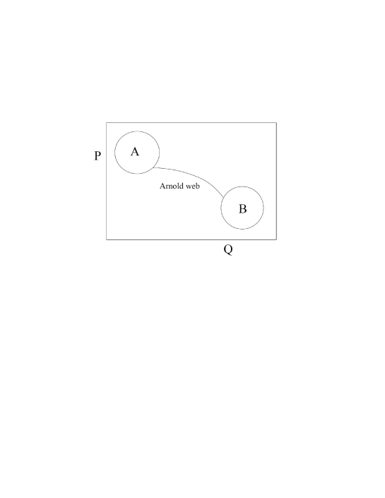
Figure 3: A schematic representation of the phase-space. Regions A and B communicate via the Arnold web.

In the idealized case of a phase fluid set from the start to satisfy the above condition, the above version of Jeans’ theorem corresponds essentially to the preservation of the phase space density under the system’s Hamiltonian flow. In practice, however, a definition of ‘well-connected’ region such as the above one, i.e., based only on topological arguments, may not be so convenient in describing galactic equilibria. We can give the following qualitative argument: Suppose the 6D phase space of a galactic system is represented schematically as the $(Q,P)$ space of Fig.3. Suppose also that the system’s Hamiltonian $H$ differs from an integrable Hamiltonian, with exact integrals $I_{1},I_{2},I_{3}$, by an arbitrarily small perturbation, of order $O(\epsilon)$. According to Nekhoroshev theorem, if $\epsilon$ is below a threshold, there are approximate integrals $\tilde{I}_{1},\tilde{I}_{2},\tilde{I}_{3}$ that have variations of order $O(\exp(-1/\epsilon))$ over timescales of order $O(\exp(1/\epsilon))$, i.e., much longer than the age of the galaxy. Thus, for all practical purposes, we may describe the system by a distribution function depending on these approximate integrals $f(\tilde{I}_{1},\tilde{I}_{2},\tilde{I}_{3})$. Consider now two different regions of $(Q,P)$, region A and region B (Fig.3), with an $O(1)$ separation in phase-space (in units normalized to the overall extent of the phase space in $P$ and $Q$). As a consequence, the values of $\tilde{I}_{i}$, which are functions of the variables $(Q,P)$, will in general also have an $O(1)$ difference in the two regions, that is $|\tilde{I}_{i}(A)-\tilde{I}_{i}(B)|=O(1)$ . Since these integrals are arguments of the distribution function, it follows that the same order of the difference will also appear in $f$, that is

$$|f(A)-f(B)|=O(1)~{}~{}.$$ (40)

Given, now, that the Nekhoroshev theorem for approximate integrals is valid in open domains of the phase space, it follows that Eq.(40) is valid for $f(A),f(B)$ standing for the value of the distribution function at any pair of points inside the regions A and B respectively, provided that the approximate integrals $\tilde{I}_{i}$ are well preserved in both regions. On the other hand, according to the KAM theorem (Kolmogorov 1954, Arnold 1963, Moser 1962), there is a chaotic subset of measure $O(\epsilon)$ in region A, which is the compement of the invariant tori of A, and a similar subset in region B. Suppose that the two subsets communicate via the Arnold web. Then, according to the previous definitions, the two subsets belong to one ’well-connected’ chaotic region and we should have $f(A)-f(B)=0$ for any pair of points in A and B belonging to this region. Thus we see that if we use the approximate integrals $\tilde{I}_{i}$ as arguments in the distribution function we reach a different conclusion (Eq.(40)) than if we use the concept of well-connectedness. This is because the integrals $\tilde{I}_{i}$ are not exact, but they are preserved for times of the order of the Nekhoroshev time $t_{Nek}$. Thus the equalization of $f(A)$ and $f(B)$ in the chaotic subset can happen only after a time $t>t_{Nek}$, which is much larger than the age of the system.

The above example shows that a more pragmatic definition of what ‘well-connected’ means is required in the case of galaxies, in order to take into account the fact that the topological well-connectedness may not have always practical dynamical implications for the equilibria of galaxies. This is because the lifetime of galaxies is much smaller than the typical Nekhoroshev time.

A numerical example of the form of the distribution function in systems with divided phase space was given by analyzing the orbits and approximate integrals in the phase space of systems produced by N-Body simulations (Efthymiopoulos 1999, Contopoulos et al. 2000, Efthymiopoulos and Voglis 2001, Contopoulos et al. 2002). Fig.4 (Contopoulos et al. 2000) shows one example of a nearly prolate system. This system resulted from a collapse simulation with cosmological initial conditions (Efthymiopoulos and Voglis 2001). The self-consistent gravitational potential is calculated by the self-consistent field code of Allen et al. (1990). If we ignore triaxial terms, the potential can be expanded in a polynomial series in the $(R,z)$ variables, namely:

$$\Phi(R,z)=\sum_{k=0}^{8}\sum_{l=0}^{8}g_{kl}R^{2k}z^{2l}$$ (41)

where $z$ is the long axis of the system and the coefficients $g_{kl}$ are specified numerically, via the code potential. The form of the potential (41) is such that a third integral can be calculated in the form of series. We calculate a different integral for box orbits (non-resonant integral) or for higher-order resonant orbits (e.g. 1:1 resonance for tube orbits).

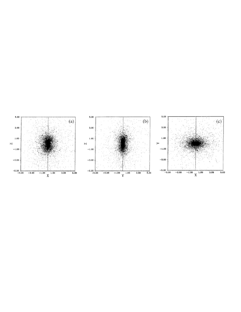
Figure 4: Projection of the final state of an N-Body collapse experiment in the three planes (a) X-Z, (b) Y-Z, (c) X-Y of ordinary space. The system is nearly prolate, with one long axis (Z) and two short axes (X,Y) (after Contopoulos et al. 2000).

The question, now, is whether such integrals should appear as arguments in the distribution function of the system. The answer is affirmative, as indicated by Fig.5. Panel (a) shows a Poincaré surface of section $(R,\dot{R})$ for an energy $E=-1.6\times 10^{6}$ (in the N-Body units) which is close to the central value of the potential well ($-2\times 10^{6}$), and angular momentum $L_{z}$ close to zero. We then integrate the orbits of the real particles of the N-Body system with energies in a bin centered at the above value of $E$, until each orbit intersects the Poincaré section for the first time. By this numerical process, a particle located on an invariant torus of the system, that corresponds to a particular value of the third integral $I$, is transferred to a point on an invariant curve of the section $(R,\dot{R})$ where the section is intersected by the torus. This also means that if the phase-space density (distribution function $f$) depends on $I$, the surface density of points in the section $(R,\dot{R})$ will also be stratified in such a way that the equidensities should coincide with the invariant curves corresponding to different label values of $I$. Precisely, this is what we see in Fig.5b. Namely, the equidensity contours of the distribution of the real particles in the surface of section have a good coincidence with the invariant curves (shown together in Fig.5c). This is a numerical indication that the integral $I$ should, indeed, be included as an argument in $f$ (see also Contopoulos et al. 2002). We have calculated numerically the dependence of the surface density $f_{S}$ on $I$ and found it to be exponential (Fig.5d).

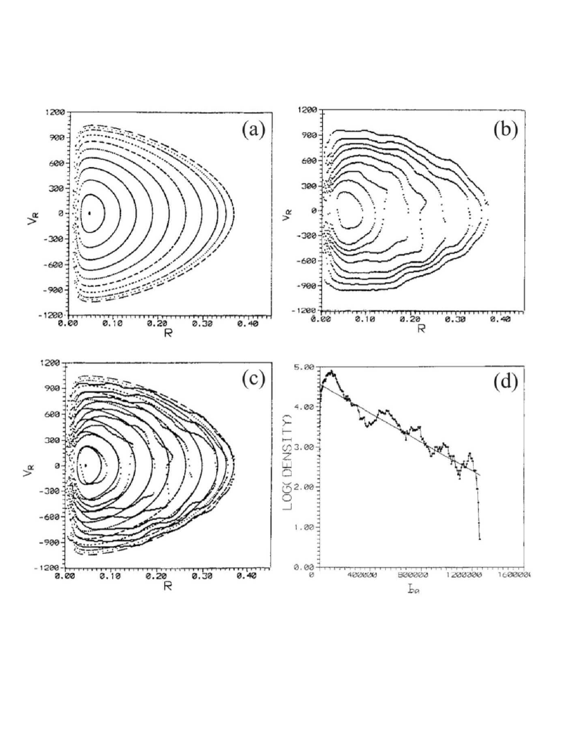
Figure 5: (a) The Poincaré surface of section of the system of Fig.4 for energy $E=-1.6\times 10^{6}$ (in the N-Body units) and $L_{z}$ very close to zero $L_{z}=0.045$. (b) The equidensity contours of the distribution of the real particles in the Poincaré section, for energies within a bin $\Delta E=2\times 10^{4}$ around the value $E$ of (a) and angular momentum $|L_{z}|\leq 0.09$. (c) the plots (a) and (b) together. (d) Exponential dependence of the distribution function on the value of the third integral along the invariant curves of (a) (after Contopoulos et al. 2000).

For larger energies, the divided nature of the phase-space is clearly manifested (Fig.6a). In particular, besides the region of invariant curves corresponding to box orbits (A), we distinguish a second island around the 1:1 resonance (B) as well as a connected chaotic domain (C) separating the two regular domains. Some finer details, e.g., secondary resonances (D) are distinguished but they are not dynamically so important. If, now, we compare this figure to the equidensity plot of the distribution of particles (Figs.6b,c), the tendency to have a distribution stratified according to the underlying phase-space structure is again visible to a large extent. This indicates that both the non-resonant third integral, yielding the tori of region (A), and the resonant integral yielding the tori of (B), should appear locally as arguments of the distribution function $f$ (the dependence of $f$ on $I$ in region A is again exponential, Fig.6d).

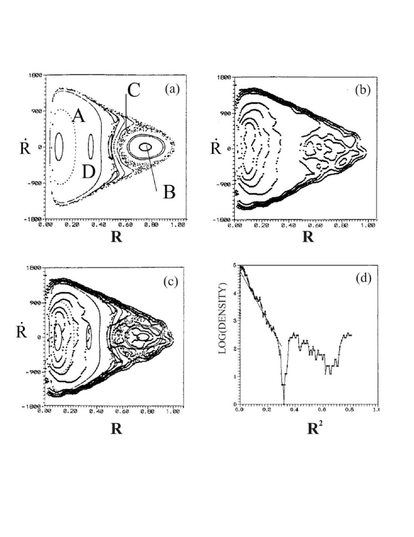
Figure 6: As in Fig.5, for a different value of the energy ($E=-9\times 10^{5}$). The region (A) corresponds to box orbits, (B) to loop orbits (1:1 resonance), (C) chaotic orbits, and (D) a secondary resonance inside the domain of box orbits. In (d) we use the approximation $I\propto R^{2}$ (after Contopoulos et al. 2000).

For still larger energies, the chaotic domain occupies a large volume of the phase space (Fig.7a). We find that the phase-space density of the real particles in the connected chaotic domain is nearly constant. Fig.7b shows the density on the Poincaré section along a constant line $R=0.65$, as a function of $\dot{R}$. The variations shown in Fig.7b are not completely due to the sampling noise, but, in general, they are small enough so as to allow us to characterize the density as nearly constant in the connected chaotic domain (C). In this case Merritt’s version of Jeans’ theorem is applicable.

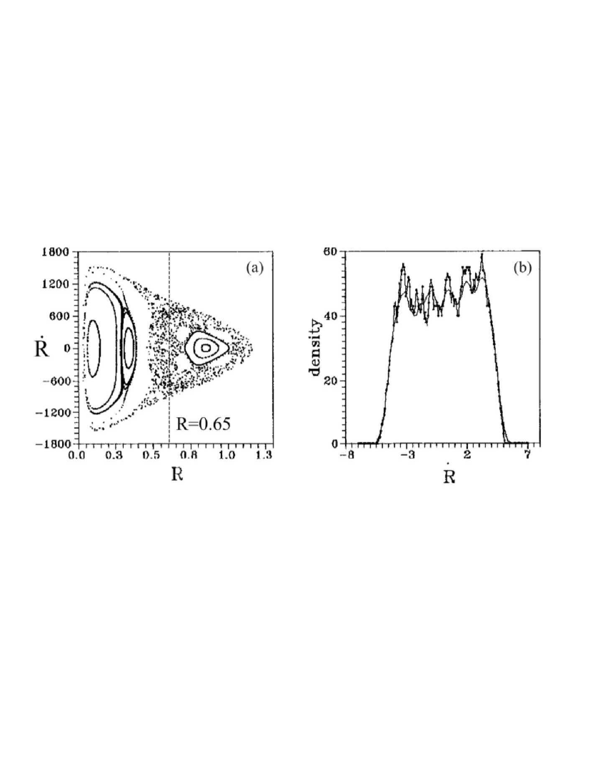
Figure 7: (a) As in Fig.5a for energy $E=-8\times 10^{5}$. (b) the density of real particles of the N-Body system in a slice around the line $R=0.65$ is almost constant (after Contopoulos et al. 2000).

The nature of the above questions prevents one from making clearcut statements as per what phenomena introduced by regular or chaotic orbits should be considered as dynamically important. Let us notice, however, that galaxies are quite complex systems and such questions have not yet been fully explored even in simple toy models of basic research in Hamiltonian dynamical systems. We mention one example which is of particular importance in the study of global dynamics of galaxies: the distinction between Arnold diffusion (Arnold 1964) and resonance overlap diffusion (Contopoulos 1966(7), Rosenbluth et al. 1966, Chirikov 1979) and the role of these two types of diffusion in galaxies. The difference between these two types of diffusion is topological, but it is also a difference in the diffusion rate. As regards the rate of Arnold diffusion, there is a general belief that this should be connected to Nekhoroshev theorem and that, hence, it is very slow to be of any importance in galaxies. This was partly verified recently by the interesting numerical experiments of Froeschlé and his collaborators (Froeschlé et al. 2000, Guzzo et al. 2002, 2005, Lega et al. 2003). More work is requested in order that such simulations help us clarify questions such as what is a pragmatic definition of ‘well-connected’ domains of phase space and how to implement such ideas in galactic dynamics.

3 The Statistical Mechanical Approach - Violent Relaxation

3.1 Observational evidence of the equilibrium state assumption

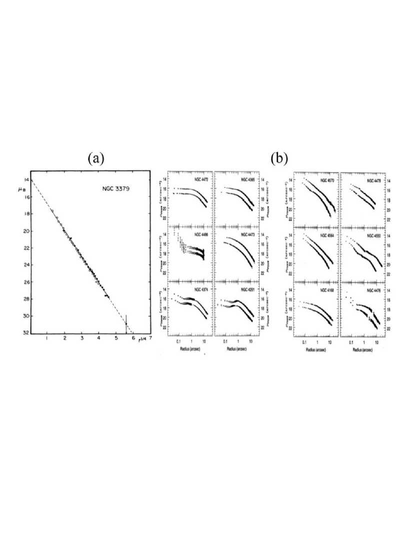
Figure 8: (a) Fitting of the elliptical galaxy NGC3379 by de Vaucouleurs’ law (after de Vaucouleurs and Capaccioli 1979). (b) Shallow (left) and cuspy (right) profiles of the cores of elliptical galaxies (after Ferrarese et al. 1994).

The smoothness of observed photometric profiles suggests that at least the spheroidal components of galaxies are in a form of statistical equilibrium. The surface brightness profiles of many elliptical galaxies are well-fitted by the de Vaucouleurs’ (1948) $R^{1/4}$ law (Fig.8a):

$$I(R)=I_{e}\exp\big{(}-7.67[(R/R_{e})^{1/4}-1]\big{)}$$ (42)

where $I_{e}$ is the value of the surface brightness (in $mag/arcsec^{2}$) at the radius $R_{e}$ of a disk in the plane of projection containing half of the total light. In a number of galaxies this relation is verified in a range up to ten magnitudes (e.g. de Vaucouleurs and Capaccioli 1979). The profiles of bulges and of some ellipticals follow a similar law, namely the Sersic $R^{1/n}$ law (Sersic 1963, 1968). On the other hand, the central profiles of elliptical galaxies were reliably observed by the Hubble space telescope. It was found that the profiles have central cusps, i.e., the surface brightness grows as a power-law in the center $I(R)\propto R^{-\gamma}$, $\gamma>0$ (Crane et al. 1993, Ferrarese et al. 1994, Lauer et al. 1995). There are two groups of observed central profiles (Fig.8b), namely a) shallow profiles ($\gamma\leq 0.2$), and b) abrupt profiles ($\gamma\sim 1$). However, as emphasized by Merritt (1996), even shallow profiles in the surface brightness correspond to power-law cusps in the 3D density profile $\rho(r)\propto r^{-a}$ with power exponents $a>1$. This means that at least the centers of galaxies deviate considerably from simple isothermal models with a Boltzmann - type distribution function such as the King models (King 1962):

$$f(\mathbf{x},\mathbf{p})=A\exp\left[-\beta\left(E(\mathbf{x},\mathbf{p})-E_{0}\right)\right]=A\exp\left[-\beta\left({\mathbf{p}^{2}\over 2}+\Phi(\mathbf{x})-E_{0}\right)\right]$$ (43)

with $A,\beta,E_{0}$ constants, or their non-isotropic generalizations (Michie 1963). The latter models are characterized by flat density profiles at the center (Binney and Tremaine, 1987, p.234). Thus, the nature of statistical equilibrium of galaxies should be quite different to the isothermal equilibrium. Furthermore, since the time of two-body relaxation is much larger than the age of the Universe, galaxies had no time to approach such an equilibrium. The very fact that galaxies are statistically relaxed systems seems, at first, to be a paradox (the so-called ‘Zwicky’s paradox’).

3.2 The theory of violent relaxation

A way out of the paradox developed gradually in the sixties, after a systematic study of the hypothesis that in the early phase of galaxy formation, galaxies were subject to a sort of ‘violent relaxation’ (Lynden-Bell 1967) caused by the collapse and ultimate merger of clumps of matter produced by the nonlinear evolution of initially small density inhomogeneities in the early Universe. We can mention in this context an influential paper by Eggen, Lynden-Bell and Sandage (1962) under the characteristic title “Evidence from the Motions of Old Stars that the Galaxy Collapsed”, as well as one of the first numerical simulations of a spherical gravitational system in the computer by M. Hénon (1964).

The theoretical foundations of the statistical mechanics of violent relaxation were set by Lynden-Bell (1967), using a continuum approach for the distribution function, and re-derived by Shu (1978) with a particle approach to the same distribution. These analytical studies are now considered classical, despite the fact that the so-derived equilibrium distribution functions are far from able to account for the properties of systems produced by realistic N-Body simulations or for the data of observed galaxies in the sky.

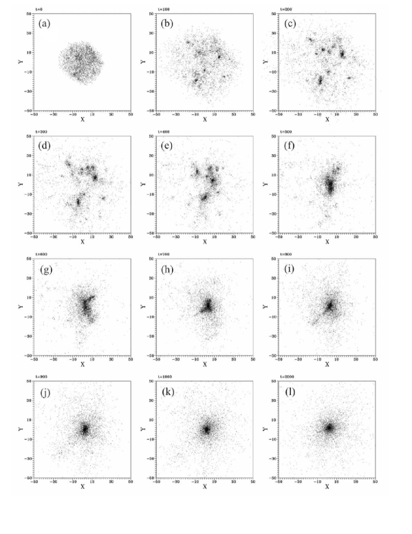
Figure 9: N-Body simulation of the collapse and violent relaxation of a nearly spherical mass (protogalaxy). The initial conditions correspond to a hierarchical clustering scenario (clumpy initial conditions) in a $\Lambda-$CDM expanding Universe (after Efthymiopoulos and Voglis 2001).

An example of such a collapse process is shown in Fig.9 (Efthymiopoulos and Voglis 2001). This is an N-Body simulation of an isolated system containing one galactic mass represented with 5616 particles. The mass is initially contained in a nearly spherical subvolume of the Universe. The particles are assigned positions and velocities in agreement with the general Hubble expansion of the Universe in a $\Lambda-$CDM scenario, but the position and velocity vectors of each particle are perturbed according to a prescription for the spectrum of density perturbations in the Universe at the moment of decoupling, and following a well-known technique of translating these perturbations into perturbations of positions and velocities introduced by Zel’dovich (1970). As seen in Fig.9, the system initially expands following the general expansion of the Universe (Figs.9a,b), but the extra gravity due to local overdensities results in a gradual detachment of the system from the average Hubble flow, so that the system reaches a maximum expansion radius (Fig.9c) and then begins to collapse. At the initial phase of collapse, small subclumps are formed within the spherical volume which collapse to local centers forming larger bound objects (Figs.9d,e). However, these clumps also collapse towards a common center of gravity (Fig.9f), until the overall system relaxes, after a phase of rebound, to a final equilibrium (Figs.9g-l).

There is a wide variety of initial conditions that lead to the above type of relaxation process. For example, a currently popular scenario of formation of elliptical galaxies via the merger of spiral galaxies (Toomre and Toomre 1972, Gerhard 1981, Negroponte and White 1983, Barnes 1988, 1992, Hernquist 1992, Naab et al. 1999, Burkert and Naab 2003) corresponds to a case where, instead of many clumps, as in Fig.9, we have only two major clumps corresponding to the dark halos of the spiral galaxies. In that case the presence of gas dynamical processes must be taken into account. Nevertheless, the main process driving the system towards a final equilibrium state is again a violent relaxation process, although the initial conditions and the detailed time evolution of the system is different than in the case of a simple collapse or a multiple merger event.

The statistical mechanical theory of violent relaxation aims, precisely, at justifying theoretically the tendency of such systems to settle down to an equilibrium, and to find the form of the distribution function $f$ at this equilibrium.

A simplified version of the main steps in the derivation of Lynden-Bell’s statistics is the following:

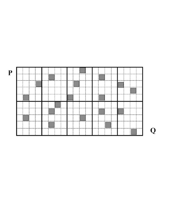
Figure 10: A simple schematic representation of the phase-space (Q,P) of a violently relaxing system. The gray squares represent elements of the phase fluid. The phase-space is partitioned in micro-cells (fine grid of dashed lines) and macro-cells (coarse grid of bold lines).

1) We consider a compact $\mu-$space (i.e. we consider that escapes are negligible), and implement a coarse - graining process by dividing the $\mu-$space in a number of, say, $N$ macrocells of equal volume (Fig.10) labelled by an index $i=1,2,...,N$. We further divide each macrocell into a number of microcells that may or may not be occupied by elements of the Liouville phase flow of the stars moving in $\mu-$space. In Fig.10 these phase elements are shown by dark squares that occupy some microcells within each macrocell.

2) We adopt the equal a priori probability assumption, namely we assume that each element of phase flow has equal a priori probability to be found in any of the macrocells of Fig.10. As the system evolves in time, each phase element travels in phase space by respecting this assumption. We should note that, because of phase mixing, the form of the phase elements also changes in time. However, this deformation does not change the volume of an element. We can thus proceed in counting the number of phase elements in each macrocell by keeping the simple schematic picture of Fig.10.

3) We denote by $n_{i}$ the occupation number of the i-th macrocell, i.e., the number of fluid elements inside this macrocell at any fixed time $t$. The set of numbers $(n_{1},n_{2},...,n_{N})$, called a macrostate, can thus be viewed as a discretized realization of the coarse-grained distribution function of the system at the time $t$.

4) For any given macrostate, the mutual exchange of any two phase elements, or the shift of an element in a different cell within the same macrocell leaves the macrostate unaltered. Thus, we can calculate the number $\Omega(n_{1},n_{2},...,n_{N})$ of all possible microscopic configurations that correspond to a given macrostate, and define a Boltzmann entropy $S=\ln\Omega$ for this particular macrostate. If we denote by $n=\sum_{i=1}^{N}n_{i}$ the total number of phase elements and by $\nu$ the (constant) number of microcells within each macrocell, the combinatorial calculation of $\Omega$ readily yields:

$$\Omega(n_{1},n_{2},...,n_{N})={n!\over n_{1}!n_{2}!...n_{N}!}\prod_{i=1}^{N}{\nu!\over(\nu-n_{i})!}$$ (44)

5) We finally seek to determine a statistical equilibrium state as the most probable macrostate, i.e., the one maximizing $S$ under the constraints imposed by all preserved quantities of the phase flow. Besides mass conservation $n=\sum_{i=1,N}n_{i}$, we can assume conservation of the total energy of the system $E=\sum_{i=1}^{N}n_{i}\epsilon_{i}$ (where $\epsilon_{i}$ is the average energy of particles in the macrocell $i$), and perhaps of other quantities such as the total angular momentum (if spherical symmetry is preserved during the collapse) or any other ‘third integral’ of motion. In the simplest case of mass and energy conservation, we maximize $S$ by including the mass and energy constraints as Lagrange multipliers $\lambda_{1}$, $\lambda_{2}$ in the maximization process, namely:

$$\delta\ln\Omega-\lambda_{1}\delta n-\lambda_{2}\delta E=0$$ (45)

We furthermore apply Stirling’s formula for large numbers $\ln N!\approx N\ln N-N$. In view of Eq.(44), Eq.(45) then yields

$$F_{i}={\eta n_{i}\over\nu}|_{S=max}={\eta\over\exp(\lambda_{1}+\lambda_{2}\epsilon_{i})+1}$$ (46)

where $\eta$ is the (constant) value of the phase-space density inside each moving phase-space element. Eq.(46) is Lynden-Bell’s formula for the value $F_{i}$ of the coarse-grained distribution function within the i-th macrocell at statistical equilibrium. Following the conventions of thermodynamics, we interpret $\lambda_{2}$ as an inverse temperature constant $\lambda_{2}\equiv\beta\propto 1/T$ and $\lambda_{1}$ in terms of an effective ‘chemical potential’ $\epsilon_{0}=-\lambda_{1}/\beta$ (or ‘Fermi energy’). We thus rewrite Eq.(46) in a familiar form reminiscent of Fermi-Dirac statistics

$$F_{i}={\eta\over\exp[\beta(\epsilon_{i}-\epsilon_{0})]+1}={\eta\exp[-\beta(\epsilon_{i}-\epsilon_{0})]\over 1+\exp[-\beta(\epsilon_{i}-\epsilon_{0})]}$$ (47)

by recalling, however, that the energy and effective chemical potential in Eq.(47) have in fact dimensions of energy per unit mass, in accordance to our general treatment of orbits in $\mu-$space (subsection 2.2). Therefore, contrary to two-body relaxation, the process of violent relaxation cannot lead to mass segregation at the equilibrium state. At any rate, in the so-called non-degenerate limit $F_{i}<<\eta$, Eq.(47) tends to the form of a Boltzmann distribution $F_{i}\simeq A\exp(-\beta\epsilon_{i})$, that is, the final state approaches the isothermal model.

The above exposition of Lynden-Bell’s theory is simplified in many aspects. In particular: a) The expression given for the constraint in the total energy is not precise. One should calculate the energy self-consistently by the gravitational interaction of the masses contained in each phase element. However, the final result turns out to be the same with this more precise calculation. b) All phase elements in the above derivation are assumed to have the same value of the phase space density $\eta$, i.e., the same ‘darkness’ in Fig.10.

A more general distribution function was derived by Lynden-Bell when the phase elements of Fig.10 can be grouped into $K$ groups of distinct darkness $\eta_{J}$, $J=1,\ldots K$. The final formula, derived also by the standard combinatorial calculation, reads:

$$F_{i}=\sum_{J=1}^{K}{\eta_{J}\exp\big{(}-\beta_{J}(\epsilon_{i}-\epsilon_{0J})\big{)}\over 1+\sum_{J=1}^{K}\exp\big{(}-\beta_{J}(\epsilon_{i}-\epsilon_{0J})\big{)}}$$ (48)

that is, it depends on a set of $K$ pairs of Lagrange multipliers $\beta_{J},\epsilon_{0J}$, $J=1,\ldots,K$. This more realistic formula links the initial conditions of formation of a system, parameterized by the values of $\eta_{J}$ which are conserved during the relaxation, to the final distribution function. In the non-degenerate limit, the latter is a superposition of nearly Boltzmann distributions, meaning that each group of phase elements is characterized by its own Maxwellian distribution of velocities which yields a different velocity dispersion in each group, depending on the value of $\eta_{J}$ This poses a problem as regards the possibility to express the overall distribution of velocities in the galaxy by a single Maxwellian function. (see for example Shu 1978 and the debate Shu 1987 - Madsen 1987). We return to this question in subsection (3.5) where we discuss alternative formulations of the statistical mechanics of violently relaxing systems.

3.3 Incomplete relaxation

The basic prediction of Lynden-Bell’s theory, namely the possibility for a stellar system to settle down to a statistical equilibrium within a time comparable to a few system’s mean dynamical times, has been completely verified in a series of numerical simulations over subsequent years (e.g. Gott 1973, 1975, White 1976, 1978, Aarseth and Binney 1978, Hoffman et al. 1979, van Albada 1982, 1987, May and Van Albada 1984, McGlynn 1984, Villumsen 1984, Aguilar and Merritt 1990, Burkert 1990, Mineau et al. 1990, Katz 1991, Dubinski and Calberg 1991, Londrillo et al. 1991, Cannizzo and Holister 1992, Curir et al. 1993, Voglis 1994a, Voglis et al. 1995, Carpintero and Muzzio 1995, Henriksen and Widrow 1997, 1999, Efthymiopoulos and Voglis 2001, Merrall and Henriksen 2003, Trenti et al. 2005). However, the data of these experiments, as well as other considerations converge to the conclusion that Lynden-Bell’s formula (47) is not applicable even in the simplest cases of realistic galactic systems (Cuperman et al. 1969, Goldstein et al. 1969, Lecar and Cohen 1972, White 1976, Binney 1982b, May and Van Albada 1984, Severne and Luwel 1986, Madsen 1987, Hjorth and Madsen 1991, Voglis et al. 1991, Voglis 1994a, Takizawa and Inagaki 1997, Efthymiopoulos and Voglis 2001, Trenti et al. 2005).

There are many phenomena which act as factors of obstruction to a convergence of $F$ towards Lynden-Bell’s prediction. We refer below to one of the most important factors considered in the literature: incomplete relaxation. This is a phenomenon that may happen even in the simplest case of systems relaxing via a monolithic collapse. The term ‘incomplete’ means that the process of mixing of phase elements in $\mu$ space, during the relaxation process, is not efficient enough so as to justify the assignment of equal a priori probability on a phase element to be in any of the macrocells of $\mu$. This also implies that some memory of initial conditions survives in the final equilibrium state. This phenomenon is commonly verified by N-Body experiments (May and Van Albada 1984, Stiavelli and Bertin 1987, Voglis et al. 1991, 1995, Efthymiopoulos and Voglis 2001, Trenti et al. 2005). An example is shown in Fig.11 (Voglis et al. 1995) which shows a plot of the final versus initial energies (Fig.11a) or angular momenta (Fig.11b) for each particle in a N-Body collapse experiment. The correlation between initial and final values of the angular momentum is obvious from the concentration of points towards the diagonal.

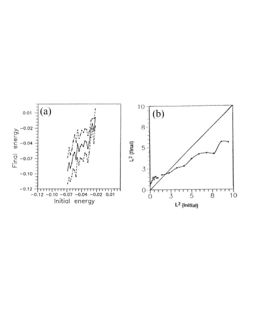
Figure 11: (a) Initial versus final energies (solid line=mean, dashed lines = lower and upper limits) of the particles before and after the collapse. (b) Initial versus final angular momenta for the same particles (after Voglis et al. 1995).

We may quantify this correlation by calculating, in N-Body collapse experiments, the time-dependence of the correlation coefficient defined by

$$CR(t)={\sum_{i=1}^{N}(E_{0i}-\bar{E}_{0})(E_{ti}-\bar{E}_{t})\over\sqrt{\sum_{i=1}^{N}(E_{0i}-\bar{E}_{0})^{2}\sum_{i=1}^{N}(E_{ti}-\bar{E}_{t})^{2}}}$$ (49)

where $E_{0i}$ , $i=1,...,N$ are the energies of the N particles at the initial snapshot of the experiment, $E_{ti}$ the energies of the same particles (each labelled by $i$) at a time $t$, and $\bar{E}_{0}$, $\bar{E}_{t}$ the mean energies respectively (Fig.12). In this and in subsequent plots we refer to a series of collapse experiments corresponding to the time evolution of the matter distributed in a spherical volume in the Universe containing one galactic mass, in which, at the moment of decoupling, we impose a field of density perturbations consistent with a standard $\Lambda-$ CDM cosmological scenario. We furthermore distinguish between a) experiments with a spherically symmetric field of initial density perturbations, and b) clumpy initial density perturbations (S and C experiments, see Efthymiopoulos and Voglis 2001 for a detailed description of the initial conditions of the experiments). Finally, we examine various exponents $n$ of the power spectrum of density perturbations, that is, the r.m.s. dependence of a density perturbation on scale $r$ is given by

$${\delta\rho(r)\over\rho}\propto{1\over r^{n+3\over 2}}$$ (50)

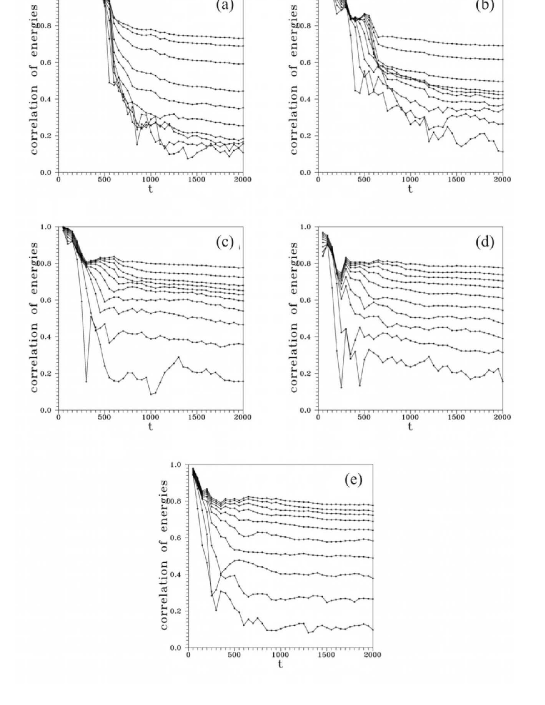
Figure 12: The time evolution of the initial - final energy correlation coefficient (Eq.(49)) for five collapse experiments differentiated by the value of the power exponent $n$ of initial density perturbations, namely (a)$n=-2.9$, (b)$n=-2$, (c)$n=-1$, (d)$n=0$, (e)$n=1$. The curves in each panel from down to the top correspond to the values of the correlation coefficient for the innermost 10%,20%,…90% of the bound matter.

according to standard cosmological considerations (see Voglis 1994b). In the case of S-experiments, Eq.(50) is viewed as the radial profile of a spherically symmetric density perturbation, while in the C-experiments the perturbation field inside the spherical volume is determined by a superposition of plane waves with power spectrum $P(k)\propto k^{n}$ and random phases. The resulting perturbation field is translated to perturbation of the particles’ positions and velocities with respect to an ideal Hubble flow by means of Zel’dovich approximation (Zel’dovich 1970). We choose different values of the exponent $n$ in the range $-3<n\leq 1$, consistent with the hierarchical clustering scenario.

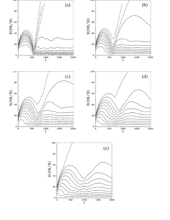
Figure 13: The time evolution of the radii of spherical shells containing 10%,20%,…90% of the matter in the same experiments as in Fig.12.

The value of $n$ is a parameter that regulates the violence of the collapse phase by affecting the distribution of power between perturbations of small and large scale. This can be seen by the following analysis, due to Palmer and Voglis (1983): if the r.m.s profile of mass perturbation in a structure of scale $h$ at the moment of cosmological decoupling is, according to Eq.(50) taken to be $\mu^{2}(h)=\mu_{0}h^{-(n+3)}$, then the total mass contained in the interior of a sphere of radius $h$, given by $M(h)={4\pi\over 3}\rho_{0}h^{3}[1+\mu(h)]$, where $\rho_{0}$ is the average density of the Universe at decoupling, will cause a gravitational attraction of the spherical shell at radius $h$ so that the expansion of the shell will gradually detach from the average Hubble expansion of the Universe. If $r(t)$ denotes the radius of the shell at the moment $t$, the solutions of the equations of motion in a $\Omega=1$ Universe can be given parametrically in the form of cycloid motion

$$r=h{1+\mu(h)\over 2\mu(h)}(1-\cos u),~{}~{}~{}t=t_{0}{3[1+\mu(h)]\over 4\mu(h)^{3/2}}(u-\sin u)$$

where $t_{0}$ is the time of decoupling, $r(t_{0})=h$, and we use units in which $G=1$ and the Hubble constant at decoupling is $H_{0}=\sqrt{2}$. From these equations we find that a shell of radius $h$ will reach its maximum expansion at $t_{max}\approx 3t_{0}\pi/4\mu(h)^{3/2}$, and from there on the shell will begin to collapse, the collapse time being almost equal to the expansion time. We may now use the form of the profile $\mu(h)\propto h^{-(n+3)/2}$ and find that the collapse time for a spherical shell including in its interior spherical volume a percentage $\Delta M\over M$ of the total mass of the system is given by:

$$t_{collapse}\propto\left({\Delta M\over M}\right)^{n+3\over 4}~{}~{}.$$ (51)

This power-law is well verified in N-Body experiments. In Fig.13 we show the evolution of the radii $r(t)$ of spherical shells containing a percentage $10\%,20\%,...,90\%$ of the total mass of the collapsing object for different values of $n$, namely a) $n=-2.9$, b) $n=-2$, c) $n=-1$, d) $n=0$, and e) $n=1$. It is immediately seen that in the limit $n\rightarrow-3$ (Fig.13a), meaning a homogeneous profile of the initial density perturbation (Eq.(50)), all shells collapse at about the same time. This is the well known spherical ‘top-hat’ model. On the other hand, as $n$ increases, the collapse becomes more gradual, and in the other limit $n\rightarrow 1$ (Fig.13e) the outer shells collapse at a time which is an order of magnitude larger than the collapse time of the inner shells.

Fig.14 shows the value of the correlation coefficient (49) of the particles’ energies at the initial and final snapshot of the experiment, as a function of the exponent $n$. There are nine curves in this diagram, corresponding to the value of the correlation coefficient for the innermost 10%, 20%, …, 90% of the matter. We see that, independently of the value of $n$, the innermost 20% of the matter yields low correlation coefficients (0.2 to 0.3), meaning that we can speak about almost complete relaxation. In the case of the $n=-2.9$ experiment, this percentage raises to 40%. However, for the rest of matter the correlation coefficient has values that can be as high as 0.7. This means that the mixing of energies is incomplete. Such high values of the correlation coefficient are observed in all the experiments, including the limit of the ‘top-hat’ model ($n=-2.9$).

Figure 14: The final value of the correlation coefficient (at $t=2000$) for the 10%, 20%,…90% of matter (from down to top) as a function of the exponent $n$ of the initial density perturbations. The correlation coefficient has relatively high values for an important fraction of the matter of all the systems, indicating that the relaxation is incomplete.

This fact is remarkable, and requires some further explanation. This is related to a problem regarding the very nature of violent relaxation that was posed by Miller (private correspondence with Lynden-Bell, see Merritt 2005). In the original approach of Lynden-Bell, the energies of stars are subject to stochastic changes caused by the time fluctuations of the self-gravitational potential of the system, since the rate of energy change of each star is given by:

$${dE\over dt}={\partial\Phi\over\partial t}$$ (52)

The rate of relaxation is thus linked to the mean timescale of the time-dependent variations in the r.h.s. of Eq.(52), that is $T_{rel}\sim<(\Phi/\dot{\Phi})^{2}>^{1/2}$. Lynden-Bell established that this timescale is of the order of the mean dynamical period of the system, hence the term ‘violent’ relaxation. Nevertheless, Miller notices that if we have an isolated galaxy and a mass $m$ which is uniformly distributed in a spherical shell surrounding the galaxy, then, if we let the mass $m$ vary in time $m\equiv m(t)$, the total gravitational potential $\Phi=\Phi_{galaxy}+\Phi_{shell}$ becomes time-dependent. As a result, the energy of each star in the galaxy changes, according to Eq.(52), but these changes are only due to the addition of a time-dependent uniform term to the energies of all stars and, in reality, they have no effect in the stars’ orbits, since the shell does not excert any force to particles in its interior. Miller concludes that Eq.(52) cannot characterize the effectiveness, or timescale, of mixing of the energies in a violent relaxation process, but other criteria must be established in order to distinguish when and how fast such a mixing actually occurs.

The results for the ‘top-hat’ case $n=-2.9$ are in certain aspects similar to Miller’s example. Since the shells collapse all at the same time, the variations of the energies of all the stars are in-phase, that is, all the stars gain or lose energy during collapse and rebound of the system, so that the mixing of energies is not very effective despite the fact that the rate of change of energies is very fast. On the other hand, in the limit $n\rightarrow 1$, the variations of energies of the stars are to a large extent out-of-phase, since the inner shells are at the rebound phase when the outer shells are still in the collapse phase (Fig.13). This is caused by the decreasing profile of mass perturbation $\mu(h)\propto h^{-2}$. At the same time, this mechanism implies that the overall time fluctuations of the potential are less violent than in the ‘top-hat’ model. As a conclusion, in both limits $n\rightarrow-3$ and $n\rightarrow 1$ the relaxation cannot be complete, although the reasons for that are different in each limit.

The question of more refined criteria characterizing the violence or effectiveness of the relaxation process is still unanswered to a large extent. A recent proposal in this direction was made by Kandrup (Kandrup 2003, Kandrup et al. 2003). When the potential has strong time fluctuations, these fluctuations introduce chaos to the relaxing system through time-dependent terms of the Hamiltonian. This happens even in a spherically symmetric, but pulsating, or collapsing, system. For example, such chaos is found in models of spherical galaxies in which the galaxy undergoes stable periodic oscillations (e.g. Louis and Gerhard 1988, Miller and Smith 1994, Smith and Contopoulos 1995). Now, in regions of phase space where chaos is prominent, the rate of mixing is determined by the Lyapunov times of the orbits of stars that move as ensembles within the phase space (Kandrup and Mahon 1994). This so-called chaotic mixing process is much faster than the phase mixing process discussed already in Lynden-Bell (1967). In Kandrup’s view the rate of chaotic mixing determines essentially the rate of approach of the system to equilibrium.

There is no direct experimental test so far, e.g. by N-Body collapse simulations, of the validity of Kandrup’s suggestion. One way to produce such tests is by a detailed exploration of plots from N-Body collapse experiments showing in detail the spreading of particles in phase space during the relaxation phase. A schematic example is given in Fig.15. If we consider a ‘frozen’ spherical potential corresponding to one snapshot of the collapse experiment, the invariant tori of the Hamiltonian of this momentary potential have the form shown schematically in Fig.15. As long as the system is not in equilibrium, the phase flow is transverse to the direction determined by the foliation of these tori (arrows in Fig.15). However, as the system approaches closer and closer to the equilibrium, the flow becomes more and more tangent to the directions defined by the foliation of the tori. This simple picture is not precise when chaotic mixing takes place. This causes irregularities of the flow both in the transverse and tangent directions that may be the dominant source of mixing. Such irregularities are distinguishable in some real plots of the phase flow in collapse experiments (e.g. Burkert 1990, Henriksen and Widrow 1997, 1999), but, to our knowledge, there has been no systematic qualitative or quantitative study of the time evolution of this flow so far.

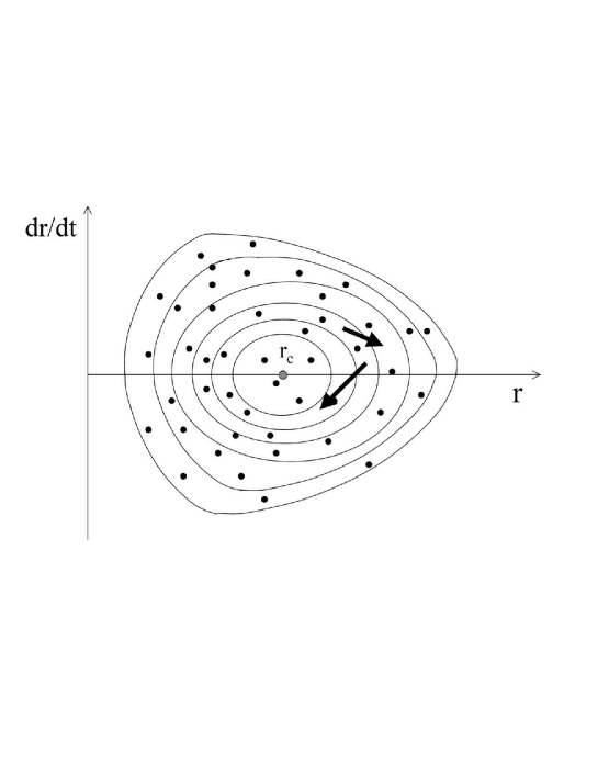
Figure 15: Schematic representation of the theoretical invariant tori in the space $r,\dot{r}$ of a spherical system for a constant pair of energy - angular momentum values. If the system is collapsing, these tori correspond to a ‘frozen’ snapshot of the time-dependent spherical potential. The relaxation process continues for as long as the phase flow of the real particles (bold arrows) is transverse to the tori. The points represent the n-body sampling of the distribution function.

3.4 Collective instabilities

Stellar systems relaxing from different initial conditions cannot in general be expected to relax to the same equilibrium endstate, since the properties of the latter are determined, to a large extent, by dynamical instabilities affecting the system in the course of or after the relaxation process. The topic of instabilities in collisionless stellar systems is a whole chapter of galactic dynamics (see Fridman and Polyachenko 1984 and Palmer 1995 for a review).

Collective instabilities in the simplest case of a spherical system where first discussed by Antonov (1960). Such instabilities may lead to interesting phenomena such as the ‘gravothermal catastrophe’ (Lynden-Bell and Wood 1968) that is believed to have played some role in dense systems such as the cores of spherical clusters. The main result of Antonov’s studies is that a spherical isotropic system is stable against radial or non-radial instabilities if its distribution function is a monotonically decreasing function of the energy (see Binney and Tremaine 1987, p.307). Subsequent studies (Hénon 1973, Dejonghe and Merritt 1988) gave criteria for the stability of anisotropic systems under various types of radial perturbations. The analog of such instabilities in the case of disks are axisymmetric instabilities (e.g. Toomre 1964).

A type of instability relevant to elongated galaxies is the ‘radial orbit instability’ (Polyachenko 1981, Polyachenko and Shukman 1984, Palmer and Papaloizou 1987). If a galaxy contains initially many radial orbits, i.e., $\sigma_{r}>>\sigma_{t}$ (subsection 2.2), a small deviation of the angular distribution of these orbits from spherically symmetric creates a collective collaboration of the orbits, based on their mutual torques, that results in a large departure of the system from the spherical symmetry. The final states can be either axisymmetric (usually prolate) or triaxial. In the case of disks, Lynden-Bell (1979) examined a similar collaboration of elongated orbits that can lead to the formation of a rotating bar inside the inner Lindblad resonance.

The general theory of the radial orbit instability is based on perturbative solutions to the collisionless Boltzmann equation. The final result can be cast in the form of Polyachenko’s criterion: a system is stable against the radial orbit instability when

$${2T_{r}\over T_{t}}\leq 1.7\pm 0.7$$ (53)

where $T_{r}=<v_{r}^{2}/2>$ and $T_{t}=<v_{t}^{2}/2>$ (in non-rotating galaxies), $v_{r}$, $v_{t}$ being the velocities of stars in the radial and transverse direction respectively. The $\pm 0.7$ error in Eq.(53) is produced by a compilation of different values of the ratio $2T_{r}/T_{t}$ reported in the literature by use of different basic models used to study the instability (see Merritt 1999, subsection 6.2 and references there in). For example, we may consider a spherical distribution function which is initially in steady state and find a somewhat different ratio $2T_{r}/T_{t}$ depending on what is the model chosen for the initial distribution function. Other, similar in spirit, criteria were proposed by different authors. For example, Merritt and Aguilar (1985) proposed the criterion $2T/|U|\leq 0.1$, where $T$ is the initial kinetic energy $U$ the initial potential energy of the system. Such criteria are verified in N-Body studies of the radial orbit instability when we start with initial conditions which are perturbations to a spherical equilibrium (e.g. Merritt and Aguilar 1985, Barnes et al. 1986, Aguilar and Merritt 1990, Canizzo and Holister 1992). If, on the other hand, we consider initial conditions corresponding to a cosmological collapse scenario (Carpintero and Muzzio 1995, Efthymiopoulos and Voglis 2001), we find that when we start with a spherically symmetric collapsing object, which has an overpopulation of radial orbits, then the system relaxes to its final equilibrium only after the ratio $2T_{r}/T_{t}$, which is initially very large, settles down to a value near Polyachenko’s value 1.7 (Fig.16a). The resulting endstates are triaxial systems with axial ratios of long to short axis corresponding to E5 - E6 galaxies. On the contrary, if we start with clumpy initial conditions (Fig.16b), which are characterized by a more random initial distribution of the directions of the particles’ velocities, the ratio $2T_{r}/T_{t}$ goes below the value $1.7$ very quickly (at $t\simeq 150$ in Fig.16b), at times smaller than the collapse time ($t_{collapse}\approx 1000$). Then the systems do not exhibit a strong radial orbit instability, and the resulting endstates resemble to E2 - E3 galaxies.

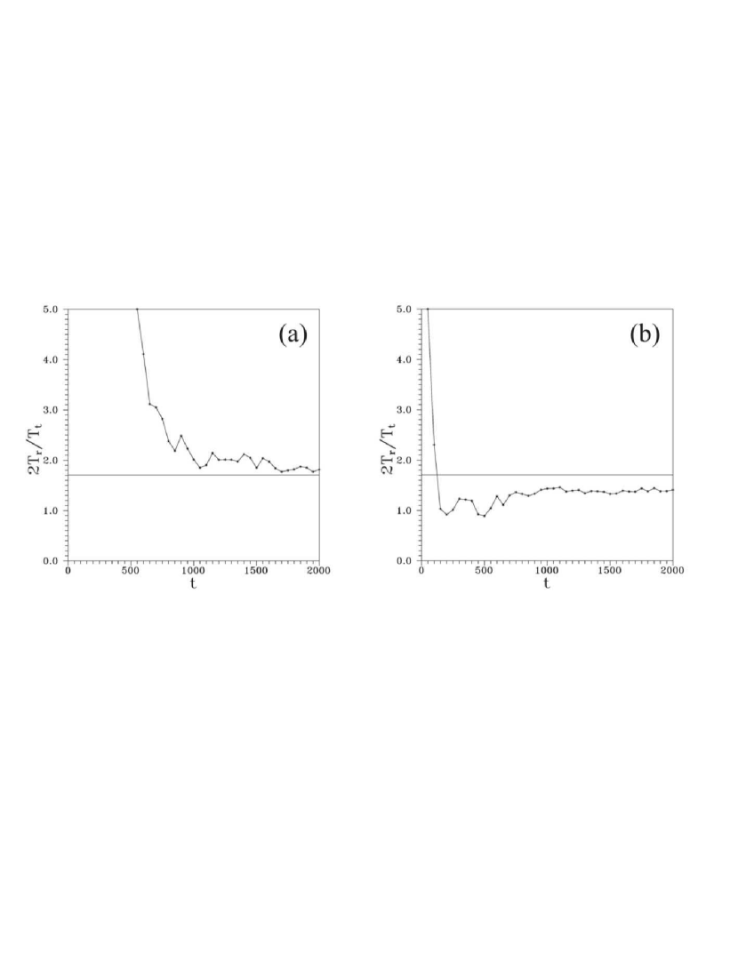
Figure 16: The time evolution of the ratio $2T_{r}/T_{t}$ in two experiments of violent relaxation from (a) quiet (spherically symmetric) initial conditions, and (b) clumpy initial conditions. For both systems, the final value stabilizes near Polyachenko’s criterion $2T_{r}/T_{t}=1.7$. Only for the system (a) the radial orbit instability is prominent.

Other types of instabilities (see Palmer 1995) are the ‘bending’ (Toomre 1966, Fridman and Polyachenko 1984, Merritt and Sellwood 1994), ‘tumbling bar’ (Allen et al. 1992) instabilities, and the bar instability in disks (Hohl 1971, Ostriker and Peebles 1973, Athanassoula and Sellwood 1986).

3.5 Alternative formulations of the statistical mechanics of violent relaxation

Both the violent relaxation process and collective instabilities processes can be described by solutions of Boltzman’s equation (see e.g. Hoffman et al. 1979, Henriksen and Widrow 1997, 1999, Merrall and Henriksen 2003 for the violent relaxation case and references in subsection (3.4) for the case of a collective instability). However, it is not clear how to distinguish between these two types of solutions, which essentially both describe excursions of a system in Liouville space, until the system settles down to a stable equilibrium state. We may say that when collective phenomena are present, these phenomena constitute the main factor determining the system’s excursion in Liouville space. The extent that this happens determines also the limits of applicability of statistical mechanical considerations such as those forming the basis of the violent relaxation theory.

On the other hand, we can always say that a stable equilibrium state of a system of many particles should correspond to a local, or global, maximum of a kind of entropy functional $S[F]$ (where $F$ is the coarse-grained distribution function). The use of such functionals to describe the endstate of a system subject to dynamical instabilities was pioneered by Ipser (1974) and Ipser and Horwitz (1979). In the case of violent relaxation, a debate was caused by a paper of Tremaine et al. (1986), supporting the view that other functionals than the Boltzman functional $S[F]=-\int F\log Fd^{6}\mu$, or its generalization by Lynden-Bell (1967) can be used in the description of statistical equilibria. In particular, any functional $S[F]$ that is convex in $F$ will be an increasing function of time that reaches a maximum at the equilibrium state, that is, it can play the role of ‘entropy’ of a stellar system. This approach to equilibrium can be measured by quantities alternative to the entropy functionals of Tremaine et al. (Mathur 1988). This point of view was immediately criticized by Kandrup (1987), Sridhar (1987) and Dejonghe (1987) on the basis of the remark that Tolman’s proof of H-theorem does not apply in the case of an arbitrary convex functional $S[F]$ and that the monotonic increase of such an ‘entropy’ cannot be established by elementary arguments. In order to resolve this issue, Soker (1996) studied in detail the time evolution of a particular choice of functional $S[F]$ which is a variant of a functional proposed by Spergel and Hernquist (1992). He found that the relaxation process can be divided in two phases: During the first phase, which includes the first collapse and rebound, the Spergel - Hernquist entropy functional may increase or decrease with time. During the second phase (called the ‘calm’ phase), it is an increasing function of time. The calm phase can perhaps be identified with the so-called ‘secondary infall’ of matter (Filmore and Goldreich 1984) that characterizes the formation of dark halos, or with the process of progressive mixing in finer and finer scales that takes place in the phase space during the late phase of relaxation.

Another class of modifications of Lynden-Bell’s statistics aims at curing the problem of superpositions of Maxwelian velocity distributions with different dispersions when the phase-space elements are divided in groups of different phase densities (subsection 3.2). Kull et al. (1997) suggested a statistical mechanics based on phase elements of unequal volumes but equal masses. They show that the resulting velocity distribution is again a superposition of Maxwellians, but this time they all have the same velocity dispersion. Nakamura (2000) made a completely different proposal in order to address the same problem. He suggested to use a particle approach for collisionless systems and defined an entropy $S=-\sum P_{i,j}\log P_{i,j}$, where $P_{i,j}$ is the probability that if a particle is at the i-th cell of the phase space at the initial time $t_{0}$, it will be at the j-th cell in the end. Numerical simulations by Merrall and Henriksen (2003) yielded the result that in collapse simulations the final velocity distribution appears to be a unique Maxwellian in the center, but in merger simulations there were considerable deviations from such a unique distribution if the centers were initially well separated. On the other hand, Arad and Johansson (2005) and Arad and Lynden-Bell (2005) made a detailed comparison of Lynden-Bell’s and Nakamura’s theories both by numerical and analytical means. The final conclusion is somewhat disappointing, since the authors support that both theories yield results not compatible with numerical experiments. Arad and Lynden Bell (2005) conclude that a proper description of the violent relaxation process should rely on dynamical arguments for the evolution of the coarse-grained distribution function rather than on the classical statistical mechanical approach.

A yet different approach is based on the search for criteria that can characterize an equilibrium of Boltzmann’s equation without reference to the concept of entropy, classical or modified. The basic proposal in this direction was made by Wiechen et al. (1988) and Ziegler and Wiechen (1989). We notice first that Boltzmann’s equation can be deduced from a Hamiltonian density function $H[f]$. Furthermore, an equilibrium state $f_{0}$ is a fixed point of $H[f]$. Ziegler and Wiechen (1989) then define a ‘dynamical energy function’ $W[f]$ such that $f_{0}$ is a minimum of $W[f]$. The difference $W[f]-W[f_{0}]$ defines a kind of energy ‘dissipated’ during the relaxation process. The same authors proposed an algorithm of calculation of the dynamical energy functional and of the state $f_{0}$. In a similar spirit, Kandrup (1998) proposed to consider the stability character of ‘orbits’ in the so-called $\Gamma$ space, the space of all states $f$, by giving a suitable definition of Lyapunov Characteristic number that is applicable to the case of the Hamiltonian density $H[f]$.

A final proposal has been to use the well known Tsallis entropy (Tsallis 1988)

$$S_{q}[f]=-{1\over q-1}\int(f^{q}-f)d^{6}\mu$$ (54)

as more relevant to the description of the relaxation process, since gravitational systems are, in general, non-extensive (Plastino and Plastino 1993, Taruya and Sakagami 2002, 2003). If the functional (54) is maximized under the usual constraints of mass and energy conservation, the resulting distribution function has the form of a polytropic distribution $f\propto|E|^{p}$, where the power index $p$ is related to the q-index of Tsallis’ entropy. This approach was criticized by Chavanis (2006), who points out the fact that the equilibria of galaxies are far from polytropic. Chavanis emphasizes that the use of the Tsallis entropy in stellar dynamics is somewhat ad hoc, because the Tsallis entropy applies when the phase space of a system is a fractal, or multifractal, while the fractal properties of the phase-space structure of stellar systems are not known. This is an open problem that requests more work to be clarified. On the other hand, Chavanis (1998, 2002) proposed a method to study the approach to equilibrium that is close in spirit to Arad and Lynden-Bell’s call upon a dynamical description of violent relaxation. The proposal is to consider a Boltzmann-type equation that describes the time evolution of either the coarse-grained distribution function $F(\mathbf{x},\mathbf{v},t)$ (Chavanis 1998), or a distribution function $\rho(\mathbf{x},\mathbf{v},\eta,t)$ that is different for each subset of phase elements with initial phase-space density equal to $\eta$ (subsection 3.2). In this studies, the analog of the partial derivative $\partial f/\partial t$ in Boltzmann’s equation (16), namely $\partial F/\partial t$ or $\partial\rho/\partial t$, is replaced by a diffusion-like term the form of which is chosen on the basis of dynamical considerations.

3.6 The number density function in the space of integrals of motion. Stiavelli - Bertin statistical mechanics

The distribution function $f$ is a density function in the six-dimensional phase space, i.e., it gives the mass of stars per unit values of the phase space coordinates. If, however, the orbits obey integrals of motion, the distribution function depends on these integrals $f\equiv f(I_{1},I_{2},...,I_{K})$, thus it can be expressed in terms of a different function, $N(I_{1},I_{2},...,I_{K})$ which yields the mass of stars $dm$ per unit value of each of the integrals $I_{i}$. The latter function, $N$, is called the number density function

$$N(\mathbf{I})={dm\over d\mathbf{I}}$$ (55)

were $\mathbf{I}$ is the K-dimensional vector of integrals considered and $d\mathbf{I}$ is an infinitesimal volume in the space of integrals. The relation between $f$ and $N$ is specified by providing the density of states function

$$W(\mathbf{I})={d\Omega(\mathbf{I})\over d\mathbf{I}}$$ (56)

where $d\Omega(\mathbf{I})$ is the elementary volume of phase space that comprises all phase-space points $(\mathbf{x},\mathbf{p})$ yielding values of the integrals in the range $\mathbf{I},\mathbf{I}+d\mathbf{I}$.

There are indications that the number density function $N$ may be more fundamental than the distribution function $f$ in the characterization of particular properties of stellar dynamical systems. A first such suggestion was made by Binney (1982b) who found that in spherical isotropic galaxies obeying de Vaucouleurs law, the number density function $N(E)$ depends exponentially on the energy $N(E)\propto\exp(-\beta E)$, a fact that allows one to characterize these systems as “isothermal after all” (Binney 1982b). In order to find the isotropic spherical equilibrium associated with de Vaucouleurs’ law (Eq.(42)), we recall that in isotropic systems only the energy $E$ appears as an argument of the distribution function $f$. We can then make use of a the well-known Eddington’s inversion formula (Eddington 1916):

$$f(E)={1\over\sqrt{8}\pi^{2}}{d\over dE}\int_{E}^{0}{d\rho\over d\Phi}{d\Phi\over\sqrt{E-\Phi}}$$ (57)

which allows one to find the unique isotropic distribution function $f(E)$ consistent with a given density - potential profile $\rho(r),\Phi(r)$ (by eliminating $r$ we use the function $\rho(\Phi)$ in the actual calculation). Since $\Phi$ is derived from Eq.(20), the only unknown of the problem is the density profile $\rho(r)$. However, we may also invert Eq.(10) and obtain $\rho(r)$ from a known surface brightness profile $\Sigma(R)$.

In the case of de Vaucouleurs’ surface brightness profile (42) we find, numerically, a particular distribution function $f(E)$. The value of $f$ is the same at all the points of phase space which lie on the same hypersurface of constant energy $E$. We next consider an elementary phase space volume $\Delta\Omega(E)=\Delta^{3}\mathbf{x}\Delta^{3}\mathbf{p}$ by taking all the points of phase space corresponding to energies in a small interval $E,E+\Delta E$. The density of states function $W(E)=\Delta\Omega(E)/\Delta E$ is then calculated. Finally, we define the number density function

$$N(E)={\Delta N\over\Delta E}={\Delta N\over\Delta\Omega}{\Delta\Omega\over\Delta E}=f(E)W(E)$$ (58)

yielding the number of particles per unit energy of the system. We stress again that $N(E)$ represents a density in energy space, while $f(E)$ represents a density in phase space. The two functions can be linked only because the distribution of velocities is isotropic. Binney’s numerical calculation showed that the number density function $N(E)$ for a system with de Vaucouleurs’ profile is, to a good approximation, an exponential function $N(E)\simeq N_{0}\exp(-\beta E)$. This suggests that a kind of statistical mechanics is applicable in these systems, which, however, should introduce a non-uniform partition of the phase-space in terms of elementary volumes $\Delta\Omega$ corresponding to the energies in intervals $E,E+\Delta E$.

This approach can be generalized in the case of anisotropic systems. In that case we consider distribution functions of the form $f(E,L^{2})$, and look for a number density distribution $N(E,L^{2})$ in the space $(E,L^{2})$, called the ‘Lindblad space’ (Merritt 1985). The calculation of the elementary volume $\Delta\Omega(E,L^{2})=\Delta^{3}\mathbf{x}\Delta^{3}\mathbf{p}$, corresponding to the volume of the union of invariant tori with energy and angular momentum values in the range $E,E+\Delta E$, $L^{2},L^{2}+\Delta L^{2}$ can be done as follows (Ogorodnikov 1965): a phase-space element corresponding to values of the phase-space variables in the range $r,r+dr$, $\theta,\theta+d\theta$, $\phi,\phi+d\phi$, $v_{r},v_{r}+dv_{r}$, $v_{t},v_{t}+dv_{t}$ (where $v_{r}$, $v_{t}$ denote the modulus of the radial and transverse velocity respectively) is given by

$$d^{3}\mathbf{r}d^{3}\mathbf{v}=r^{2}\sin\theta drd\theta d\phi 4\pi v_{t}dv_{t}dv_{r}$$ (59)

Considering the transformation $r\rightarrow r$, $\theta\rightarrow\theta$, $\phi\rightarrow\phi$, $v_{t}^{2}\rightarrow L^{2}/r^{2}$, $v_{r}^{2}\rightarrow 2[E-\Phi(r)]-L^{2}/r^{2}$, we can take the determinant of the transformation’s Jacobian matrix and write Eq.(59) in the form

$$d^{3}\mathbf{r}d^{3}\mathbf{v}=2\pi\sin\theta d\theta d\phi{dr\over v_{r}}dEdL^{2}$$ (60)

Then, the total phase space volume occupied by tori with energies in the interval $E,E+dE$ and angular momenta $L^{2},L^{2}+dL^{2}$ is given by

$$d\Omega(E,L^{2})=dEdL^{2}\pi\int_{r_{p}(E,L^{2})}^{r_{a}(E,L^{2})}{2dr\over v_{r}}\int_{0}^{\pi}\sin\theta d\theta\int_{0}^{2\pi}d\phi=dEdL^{2}4\pi^{2}T_{r}(E,L^{2})$$ (61)

where $r_{p}(E,L^{2})$, $r_{a}(E,L^{2})$ are the radii of pericenter and apocenter respectively, for given $(E,L^{2})$, that is, the roots of the equation

$$E-\Phi(r)-{L^{2}\over 2r^{2}}=0$$ (62)

and $T_{r}(E,L^{2})$ is the radial period of orbits, i.e., the time needed to go from pericenter to apocenter and back to pericenter, given by

$$T_{r}(E,L^{2})=2\int_{r_{p}(E,L^{2})}^{r_{a}(E,L^{2})}{dr\over\sqrt{2(E-\Phi(r))-{L^{2}\over r^{2}}}}$$ (63)

We thus have that:

$$W(E,L^{2})={d\Omega\over dEdL^{2}}=4\pi^{2}T_{r}(E,L^{2})~{}~{}.$$ (64)

It is remarkable that for a wide class of galactic potentials the behavior of the function $T_{r}(E,L^{2})$ is, to a very good approximation, independent of $L^{2}$, and very close to the Keplerian limit $T_{r}\propto|E|^{-3/2}$. For example, Hénon (1959) proved that the most general class of spherical potential functions for which the integral (63) is strictly independent of $L^{2}$ is the isochrone model:

$$\Phi(r)=-{GM\over b+\sqrt{r^{2}+b^{2}}}$$ (65)

and for this model Eq.(63) yields precisely the same result $T_{r}\propto|E|^{-3/2}$ as in the Keplerian case. This is also verified in the monopole terms of the potential of N-Body experiments (Voglis 1994a, Efthymiopoulos and Voglis 2001), and in the polytropic model (Palmer 1995).

In order, now, to generalize Binney’s result $N(E)\propto\exp(-\beta E)$ in the anisotropic case, we request that the number density function $N(E,L^{2})$ has exponential dependence on its arguments, that is

$$N(E,L^{2})\propto\exp\big{(}-\beta(E+b^{\prime}L^{2})\big{)}$$ (66)

On the other hand, the generalization of Eq.(58) reads:

$$f(E,L^{2})={N(E,L^{2})\over W(E,L^{2})}$$ (67)

Thus, substituting the ansatz $W\propto|E|^{-3/2}$ in Eq.(67), Eq.(66) leads to

$$f(E,L^{2})\propto|E|^{3/2}\exp\big{(}-\beta(E+b^{\prime}L^{2})\big{)}~{}~{}~{}.$$ (68)

The formula (68) was proposed by Stiavelli and Bertin (1985, 1987) as a candidate to fit the distribution function of spherically anisotropic systems. This can also be generalized to axisymmetric systems according to the formula

$$f(E,L_{z},I_{3})\propto|E|^{3/2}\exp\big{(}-\beta(E+b^{\prime}{L_{z}^{2}\over 2}+cI_{3})\big{)}$$ (69)

where we consider an axisymmetric potential

$$\Phi(r,\theta)={\zeta(r)\over r^{2}}+{\eta\cos\theta\over r^{2}}$$

which yields an integrable system third integral $I_{3}={(v_{\theta}^{2}+v_{\phi}^{2})r^{2}\over 2}+\eta\cos\theta$. A more general formula involving axisymmetric Stäckel potentials is given in Stiavelli and Bertin (1985).

The Stiavelli-Bertin distribution function can be derived on the basis of statistical mechanical considerations (Stiavelli and Bertin 1987). This is done by implementing the microcanonical approach of statistical mechanics, but assigning unequal a priori probabilities of a phase-element to visit one of the macrocells of the $\mu-$space such as in Fig.10, or partitioning this space to macrocells of unequal volume. The resulting entropy can be written in the form of a Boltzman-Gibbs entropy functional defined in the Lindblad space:

$$S[N]=-\int N(E,L^{2})\log N(E,L^{2})dEdL^{2}$$ (70)

under the usual constraints of mass and energy conservation, and one additional constraint regarding a combination of the energy and angular momentum that is quasi-preserved during the collapse (Stiavelli and Bertin 1987). The maximization of the entropy (70) leads then to an exponential law for the number density function $N(E,L^{2})$ such as in Eq.(66). A partitioning of the phase-space in terms of unequal volumes ($\propto|E|^{-3/2}$) seems quite justified by the fact that, in an integrable potential, the foliation of invariant tori create a natural partition in phase space and that, when a system is in equilibrium, there are no motions of the phase flow transverse to these tori (see discussion of Fig.15). In the next subsection we discuss the types of distribution functions found in N-Body experiments by use of similar arguments.

Independently on whether the Stiavelli - Bertin formula for $N$ is the most convenient choice or not, the important point in the above analysis is the shift of emphasis from entropy functionals depending on $f$ to entropy functionals depending on $N$, which thus becomes the important quantity to study. This point is emphasized by Tremaine (1987), see also Merritt et al. (1989). An entropy functional similar to (70) was proposed by Spergel and Hernquist (1992) in the case of isotropic spherical systems. The resulting distributions were also found in good agreement with the results of numerical experiments.

3.7 The distribution function found in N-Body experiments of violent relaxation

The number of particles used in galactic N-Body simulations has grown from $10^{4}-10^{5}$ in the 90’s to $N=10^{6}-10^{7}$ today. Even so, it remains a hardly tractable task to obtain numerically the distribution function of a relaxed system by the counting method, i.e., by counting the number of particles in cells of the six-dimensional $\mu-$space. Even a very coarse division of the phase space, say by 10 bins per dimension, would result in $10^{6}$ cells to consider, implying 1 to 10 particles per cell on average. Thus the signal would be hidden by the statistical noise.

On the other hand, with such a number of particles it is possible to do statistics in the space of integrals, or approximate integrals of motion, such as the Lindblad space $(E,L^{2})$, which has dimension equal to two, i.e., allowing for a meaningful statistics. If the system has a spherical symmetry, one can then pass from $N$ to $f$ according to the formulae of the previous subsection. Scatter plots of the positions of the particles in the space $(E,L^{2})$ can be found in a number of papers (e.g. May and van Albada 1984, Aguilar and Merritt 1990). But the first systematic study of the resulting number density function $N(E,L^{2})$ was made by Voglis (1994a), who proposed fitting formulae to represent the contours of $N$ in the space $(E,L^{2})$ (Fig.17). Similar figures were given by Natarajan et al. (1997) and Trenti et al. (2005).

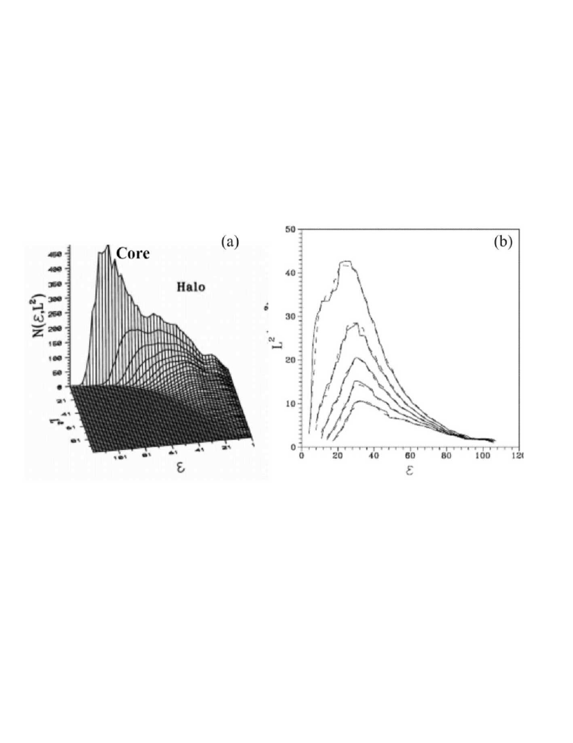
Figure 17: (a) A typical form of the ‘number density’ distribution $N(E,L^{2})$ of an N-Body system after the relaxation. (b) The contours of the function $N(E,L^{2})$ (solid line) together with the fitting by the model of Voglis 1994a (dashed line). The quantity in the abscissa is ${\cal E}=-E$ (after Voglis 1994a).

Voglis’ method gave three main results:

a) A violently relaxed system in equilibrium is characterized by the existence of a time-invariant function $N(E,L^{2})$ despite the fact that the arguments $(E,L^{2})$ are not precise integrals of motion. In particular, the energy of particles has small fluctuations due to numerical fluctuations in the coefficients of the potential of the N-Body code. On the other hand, the modulus of the angular momentum $L^{2}$ is not even approximately preserved because the final system is not spherical. Nevertheless, the function $N(E,L^{2})$ is found to remain invariant in time as a result of a ‘detailed equilibrium’ established in the space $(E,L^{2})$, namely the numbers of exchanged particles between any two elementary cells of the space $(E,L^{2})$ are equal in the course of the N-Body run.

b) The distribution $N(E,L^{2})$ is characterized by the existence of two main loci of maximum of the distribution.

The first locus, called the ‘core’ is given by pairs of values $(E,L^{2})$ which are very close to the locus of the energy of circular orbits $E_{c}(L^{2})$ if we only consider the monopole term of the multipole potential expansion of the system. The function $N(E,L^{2})$ near this maximum can be fitted by a modified Lynden-Bell’s formula:

$$N(E,L^{2})\propto{|E|^{p}\over\exp\big{(}-\beta(E-E_{c}(L^{2}))\big{)}+1}$$ (71)

where the function $E_{c}(L)$ plays the role of ‘chemical potential’. The numerator $|E|^{p}$ represents a polytropic function. The polytropic index $p$ can be shown to depend monotonically on the power-exponent of the initial density perturbation $n$ that caused the system to collapse (Efthymiopoulos and Voglis 2001).

The second locus, called ‘halo’, is in mild energies but extends to high values of the angular momentum. The associated function $E_{m}(L_{m}^{2})$ is given by two formulae relating the energy $E_{m}$ or angular momentum $L_{m}$ of the halo maximum with the value of the number density $N$ at the maximum, namely

$$\log|E|_{m}=\log{\cal E}_{0}+\nu\log\log N,~{}~{}~{}L_{m}^{2}=L_{0}^{2}(P-\log\log N)$$ (72)

with parameters ${\cal E}_{0},\nu,L_{0},P$ depending again monotonically on the exponent $n$ of density perturbations.

c) The behavior of the system near both loci indicates a local change of the sign of the temperature of the system from positive to negative. In fact, the concept of ‘negative temperature’ was introduced by Merritt et al. (1989) who had proposed ‘negative temperature’ Stiavelli-Bertin like models

$$N(E,L^{2})\propto\exp(\beta(E+b^{\prime}L^{2}))$$ (73)

i.e., with a positive factor $\beta$ appearing in the exponential dependence of $N$ on $E$. Merritt et al. (1989) suggested that such models better fit the observed surface density profiles as well as the energy distributions of violently relaxed systems. The detailed fits to numerical experiments by Aguilar and Merritt (1990) favored the negative temperature models. However, even these models failed to reproduce the N-Body distribution of particles $N(E,L^{2})$, or $N(E)$, in the region of energies close to zero. The authors suggested that this might be attributed to incomplete relaxation in the outer parts of the systems. On the other hand, Voglis’ study indicated that there is no fundamental reason to consider a unique sign of the constant $\beta$ throughout the whole available Lindblad space.

Efthymiopoulos and Voglis (2001) presented a more fundamental understanding of these results in terms of modified Stiavelli-Bertin number density statistics. In the same time, they showed that the method is applicable to systems that deviate considerably from the spherical symmetry, i.e., triaxial systems corresponding to $E5-E6$ galaxies. The key remark is that if one considers a multipole expansion of the potential written in spherical coordinates:

$$\Phi(r,\theta,\phi)=\Phi_{0}(r)+\sum_{l=0}^{\infty}\sum_{m=-l}^{l}\Phi_{lm}(r)Y_{l}^{m}(\theta,\phi)$$ (74)

where $Y_{l}^{m}(\theta,\phi)$ are spherical harmonics, then the only part of the potential which is guaranteed to yield an integrable system is the monopole term $\Phi_{0}(r)$. One can then use this term to define tori of constant label values $E,L^{2}$ under the flow induced by the Hamiltonian $H_{0}$ corresponding to $\Phi_{0}$. These, of course, are not invariant tori of the full Hamiltonian of the system. They are, however, well-defined geometrical objects in the phase space, and, therefore, they can be used in order to produce a partition of the phase space in terms of volumes $d\Omega(E,L)$ given by Eq.(60), with $\Phi_{0}$ in the place of $\Phi$. This partition is a geometrical structure, not depending on the dynamics. One can then ask what is the value of the coarse-grained distribution function $F(d\Omega)$ within each elementary volume $d\Omega$. In the case of a spherical system, this is, by definition, equal also to the value of the fine-grained distribution function $f(\mathbf{x},\mathbf{v})$ at any point $\mathbf{x},\mathbf{v}$ of $d\Omega$. In the case of an axisymmetric or triaxial system, however, $F$ is only an average value of $f$ throughout the volume $d\Omega$. We find nevertheless that $F$ can be used in the place of $f$ to reproduce the profile of the density and the profile of the anisotropy parameter $\beta$ of the system under study with very good accuracy (Efthymiopoulos and Voglis 2001).

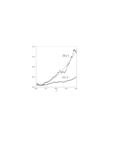
Figure 18: The Lagrange multipliers $\beta(r)$ and $B(r)$ of the ‘spherical-shell’ modified Stiavelli-Bertin statistics (Eq.(75)) for a relaxed system as functions of the distance $r$ from the center (after Efthymiopoulos and Voglis 2001).

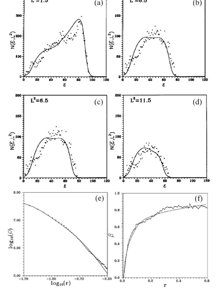
Figure 19: (a-d) Four different slices of the distribution $N({\cal E},L^{2})$ for constant angular momentum values $L^{2}=1.5,5.5,11.5$ and $29.5$. The fitting by the model of Efthymiopoulos and Voglis (2001) is shown as a solid line. (e) Reproduction of the N-Body density profile $\rho(r)$ (points) by the model (solid line) (f) same as (e) for the anisotropy parameter profile $\beta_{an}(r)$.

As regards the functional form of $F$, this is given by Eq.(67) with $F$ in the place of $f$. The problem is thus again transferred to the determination of the number density function $N(E,L^{2})$. It was found that if the system is divided in a number of spherical shells of radii $r$, width $dr$, then locally, within each shell, the number density function $\nu(E,L^{2},r)=\Delta N/\Delta E\Delta L^{2}\Delta r$ takes the form of a modified Stiavelli - Bertin’s formula

$$\nu(E,L^{2},r)={\exp\big{(}-\beta(r)E+B(r)L^{2}\big{)}\over\exp[-\beta_{c}(E-E_{a}(r,L^{2}))]+1}$$ (75)

This function fits well the numerical function $\nu(E,L^{2},r)$ found in the N-Body experiments. The latter has the same property as (a) above, i.e., it remains practically invariant in different time snapshots. The numerator of Eq.(75) has, precisely, the form of Stiavelli - Bertin statistics for the number density function (Eq.(66)). However, we find that the parameters $\beta$ and $B$, measuring the temperature and velocity anisotropy within the shell, are functions of the shell radius $r$ (Fig.18). Since these parameters enter as Lagrange multipliers in the maximization of an entropy functional in the Lindblad space, such as the functional (70), the authors concluded that the results hint towards a new type of statistics that incorporates the different degree of mixing in phase-space during relaxation between the inner and outer system’s shells. We finally note that the denominator in Eq.(75) introduces again a cut-off of the shell number density function $\nu$ for energies lower than $E_{a}(r,L)$, the energy of an orbit reaching the shell at its apocenter:

$$E_{a}(r,L^{2})={L^{2}\over 2r^{2}}+\Phi_{0}(r)~{}~{}~{}.$$ (76)

In the spherical case, Eq.(76) provides an absolute cut-off, i.e, no particle with energy $E<E_{a}$ can reach the shell. But in a triaxial system there is some tolerance around this cut-off introduced by the multipole terms of Eq.(74), which is measured by the value of the constant $\beta_{c}$.

The global number density function $N(E,L^{2})$ found by integrating $\nu(E,L^{2},r)$ over the radii of all shells

$$N(E,L^{2})=\int_{0}^{\infty}\nu(E,L^{2},r)dr$$ (77)

fitted quite nicely the numerical data in a series of experiments collapsing under either spherically symmetric or clumpy initial conditions (Figs.19a-d). The goodness of the fit was also evident in the profiles of the density $\rho(r)$ and of the anisotropy parameter $\beta_{an}(r)$ of the same systems (Fig.19e and Fig.19f respectively).

4 The orbital approach. Global dynamics and self-consistent models of galaxies

In the previous section, the focus were on studying the distribution function of galaxies on the basis of statistical mechanical considerations. However, a different approach to the same problem lies in studying the orbital content of stellar systems. An orbital study should give the main characteristics of the phase space structure and find which types have the dominant contribution in the self-consistency of the system. As a rule, a type of orbits is important if the form of the orbits supports the form of the galaxy.

In the sequel, we analyze the main types of orbits in spherical, axisymmetric and triaxial systems (we focus on non-rotating systems). We then refer to applications of ‘global dynamics’ in galaxies, based mostly on the frequency analysis of Laskar (see e.g. Laskar 1990, 1993a,b, Laskar et al. 1992, Dumas and Laskar 1993, Sidlichovsky and Nesvorny 1997, Laskar 1999, Laskar 2003). Finally, we discuss the method of self-consistent models (Schwazschild 1979) which is widely used today in order to explore the relative contribution of various types of orbits in the composition of the distribution function of a galaxy.

4.1 Orbits in spherical systems

As already discussed in subsection 2.3, the orbits in a spherical potential $\Phi(r)$ are confined to planes normal to their (constant) angular momentum vector $\mathbf{L}=\mathbf{r}\times\mathbf{\dot{r}}$. The modulus of $\mathbf{L}$ appears as a parameter in the effective one degree of freedom Hamiltonian

$$H(r,p_{r};L^{2})={p_{r}^{2}\over 2}+\Phi_{eff}(r,L)={p_{r}^{2}\over 2}+{L^{2}\over 2r^{2}}+\Phi(r)$$ (78)

with $p_{r}=\dot{r}$. The Hamiltonian (78) yields the radial motion on the orbital plane. The value $E_{c}=L^{2}/2r_{c}^{2}+\Phi(r_{c})$, where

$${d\Phi(r_{c})\over dr}-{L^{2}\over r_{c}^{3}}=0$$ (79)

yields the energy $E_{c}$ of the circular orbit with radius $r_{c}$. In galactic potentials, the radius $r_{c}$ corresponds to a minimum of the effective potential. As a result, the circular orbits are stable against radial perturbations. On the other hand, for any value of the energy $0<E\leq E_{c}$ the orbits are confined between a minimum pericentric distance $r_{p}$ and a maximum apocentric distance $r_{a}$. These are the roots of Eq.(62). The forms of the orbits are rosettes (Fig.20). The radial period is given by Eq.(63), while the azimuthal period is (e.g. Binney and Tremaine 1987, p. 107)

$$T_{\theta}(E,L^{2})=\frac{2\pi T_{r}(E,L^{2})}{\Delta\phi}$$ (80)

with

$$\Delta\phi=2L\int_{r_{p}(E,L^{2})}^{r_{a}(E,L^{2})}{dr\over r^{2}\sqrt{2(E-\Phi(r))-L^{2}/r^{2}}}$$

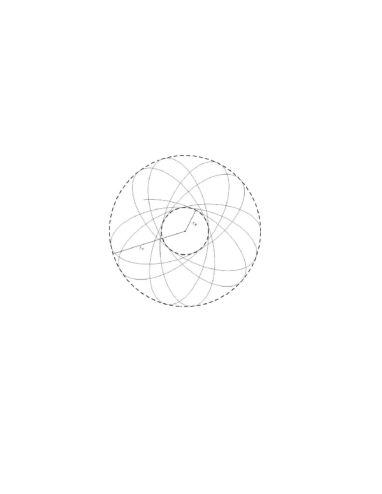
Figure 20: A typical orbit (rosette) in a spherical potential.

If the orbit is close to circular ($r_{a}-r_{p}<<r_{c}$), the radial period tends to the epicyclic period $T_{\kappa}=2\pi/\kappa$, with

$$\kappa^{2}=\frac{\partial^{2}\Phi_{eff}(r_{c})}{\partial r^{2}}={3L^{2}\over r_{c}^{4}}+{\partial^{2}\Phi\over\partial r_{c}^{2}}$$ (81)

If the density $\rho(r)$ is a decreasing function of $r$, then $1<T_{\theta}/T_{r}<2$, that is, the angle $\Delta\phi$ covered within one radial period lies between $\pi$ and $2\pi$ (Contopoulos 1954). Limiting cases are the Keplerian $\Phi(r)\propto-1/r,\rho(r)=\delta(r)$, where $\Delta\phi=2\pi$, and the homogeneous $\Phi(r)\propto r^{2},\rho(r)=const$, where $\Delta\phi=\pi$. In these potentials, there are no rosettes but only closed (periodic) orbits. In any other case, we have closed orbits if

$$\Delta\phi=\frac{m}{n}2\pi~{}~{}~{}.$$ (82)

with $m,n$ integers, $n\neq 0$.

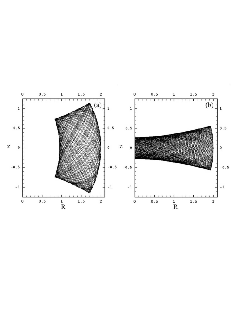
Figure 21: (a) A tube type orbit with $L_{z}\neq 0$ on the rotating meridional plane $(R,z)$ in the case of an axisymmetric potential. (b) When $L_{z}=0$ we have a box orbit. This orbit is 2D and lies on the meridional plane $(R,z)$.

4.2 Orbits in axisymmetric systems

The effective Hamiltonian of motion in the meridional plane of an axisymmetric galaxy is given by Eq.(23). We consider the potential symmetric on both sides of the plane $z=0$, $(\Phi(R,z)=\Phi(R,-z))$. All orbits preserve, besides the energy, the angular momentum component $L_{z}=R^{2}\dot{\varphi}$ which is a parameter in the two degrees of freedom Hamiltonian (23). We call $\Phi_{eff}(R,z)=\Phi(R,z)+\frac{L_{z}^{2}}{2R^{2}}$ the effective potential. The 3D orbit of a star is the result of the combination of the motion on the meridional plane $(R,z)$ and of the rotation about the $z$ axis with angular speed $\dot{\varphi}=L_{z}/R^{2}$ (which is not constant). If the orbit obeys a ‘third integral’, the orbit is called regular, otherwise it is called chaotic.

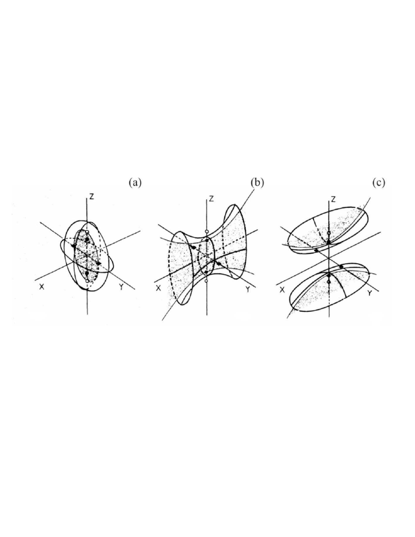
Figure 22: (a), (b), (c) Contour surfaces of constant ellipsoidal coordinates $\lambda,\mu,\nu$, respectively. The surfaces of constant $\lambda$ are ellipsoids. The surfaces of constant $\mu$ are hyperboloids of one sheet and the surfaces of constant $\nu$ are hyperboloids of two sheets (after de Zeeuw 1985).

Fig.21a shows an example of regular orbit on the meridional plane with $L_{z}\neq 0$. The model used has a potential function that corresponds to a flat central density profile. The orbit appears as a deformed parallelogram in the meridional plane. However, as the orbit also rotates, there is a cylindrical hole around the z-axis that is created by the rotation of the left boundary of the parallelogram. Such regular orbits are called ‘tubes’ (see e.g. Dehnen and Gerhard 1993). On the other hand, when $L_{z}=0$ the orbit’s left boundary touches the axis $z=0$, and the hole disappears (Fig.21b). Furthermore, there is no rotation because $\dot{\varphi}=0$. Thus, the orbits are two-dimensional, and they are called ‘box’ orbits, because their shape on the meridional plane resembles a box with curvilinear sides.

The box orbits are quasi-periodic orbits associated with two independent oscillations with incommensurable frequencies, on the $R$ and $z$ axes respectively. The limiting periodic orbits are stable orbits along the z-axis, or the R-axis. In general, the z-axis orbit is stable for values of the energy close to the central potential value. At larger values the z-axis orbit become unstables and there can be no box orbits around it. At the transition to instability, a 1:1 stable periodic orbit bifurcates from the z-axis orbit. The 1:1 orbit forms a loop on the meridional plane. Such is the orbit of figure 28c below, that corresponds to the center of the island of stability of the 1:1 resonance marked with (B) in figure 6a. Higher order periodic orbits can also exist that correspond to various ratios of the fundamental frequencies in the $z$ and $R$ axes.

In models with flat central profiles most orbits are regular (e.g. Gerhard and Binney 1985). An exploration of the phase space by means of Poincaré surfaces of section yields typically invariant curves corresponding to boxes or tubes, and only small secondary resonances with limited chaos. If, however, the galaxy has a central black hole or, more generally, a ‘Central Mass Concentration’ (CMC), the box orbits or tube orbits with low values of $L_{z}$ lose their regular character and they are converted to chaotic orbits (subsection 4.4 below).

Finally, the orbits laying on the equatorial plane follow the same rules as the orbits in spherical potentials, since they feel a 2D axisymmetric potential $\Phi(R,0)$.

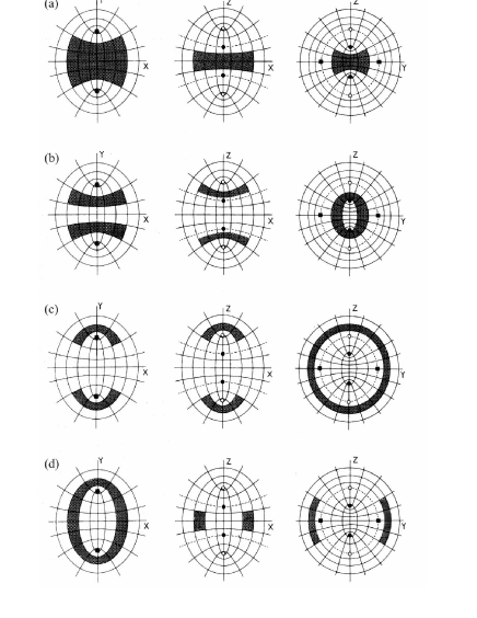
Figure 23: The cross sections of the four types of (regular) orbits with the three principal planes in the case of perfect ellipsoid Eq.(35). The coordinate surfaces confine the various types of orbits (after de Zeeuw 1985). The are (a) Box, (b) ILAT, (c) OLAT and (d) SAT orbits.

4.3 Orbits in triaxial systems

In generic triaxial models of galaxies only the energy is a global integral of motion. An exception is the perfect ellipsoid (Eq.(35)) which yields an integrable Stäckel potential (de Zeeuw 1985). The regular orbits of this model have served as a basic guide for the form of regular orbits in generic triaxial potential models. Figs.22a-c show the contour surfaces of the ellipsoidal coordinates $(\lambda,\mu,\nu)$, respectively (subsection 2.3). The surfaces of constant $\lambda$ are ellipsoids, while the surfaces of constant $\mu$ and $\nu$ are hyperboloids, of one and two sheets respectively (de Zeeuw 1985). The orbits can be of four types: a) box, b) Inner Long Axis Tube - ILAT, c) Outer Long Axis Tube - OLAT, and d) Short Axis Tube – SAT. Fig.23 shows the cross-sections of these orbits with the three principal planes as well as the limits of these orbits determined by the ellipsoidal coordinate lines.

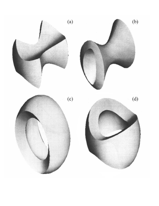
Figure 24: (a) Box, (b) ILAT, (c) OLAT, (d) SAT. The four types of (regular) orbits in 3D space (for perfect ellipsoid). These orbits are very good guides for the form of regular orbits that exist in most galactic models (after Statler 1987).

Fig.24 shows the same orbits in 3D configuration space (Statler 1987). Box orbits fill a region that resembles a parallelepiped with curved surfaces. These orbits pass arbitrarily close to the system’s center. 3D boxes do not exist in an axisymmetric configuration. On the other hand, ILATs are tube orbits which fill an elongated region around the long axis, they have a hole along the same axis and they are compatible with triaxial or prolate configurations. OLATs are tube orbits with a hole also around the long axis (like ILATs), which however do not approach close to the center of the system. OLATs are also compatible with triaxial or prolate configurations. SATs resemble like OLATs except that their hole is around the small axis. SATs are compatible with triaxial or oblate configurations. Orbits such as in Fig.21a are limiting cases of either a SAT in an oblate configuration, or an ILAT or OLAT in a prolate configuration.

Besides the above main families of orbits, in generic triaxial potentials there can be higher order periodic orbits corresponding to different commensurabilities of the basic frequencies of oscillation in the three axes (see Merritt 1999 for some examples of such orbits). When stable, these orbits are surrounded by quasi-periodic orbits which form thin tubes around the periodic orbits. We call the these orbits ‘Higher Order Resonant Tubes’ (HORT).

4.4 Chaotic orbits. The role of chaos in galaxies

The role of chaos in galaxies is currently a very active field of research (see the volume of proceedings Contopoulos and Voglis 2003). In the case of elliptical galaxies, the successful construction of self-consistent models of triaxial galaxies composed practically only by regular orbits (Schwarzschild 1979, 1982, subsection 4.6) suggested that galactic equilibria favor, for some reason, nearly-integrable models with mostly regular orbits. An explanation was provided on the basis of Statler’s (1987) self-consistent models of the perfect ellipsoid. In these models (which are integrable) there was a clear predominance of box orbits, and it was naturally expected that such a predominance should be generic. Besides the usual box orbits, which are symmetric with respect to the three axes, Levison and Richtone’s work (1987) on self-consistent models of the logarithmic potential demonstrated that there were many ‘tilted’ box orbits that were probably not associated with the axial periodic orbits, but with other higher order periodic orbits. On the other hand, Schwarzschild (1993) studied triaxial models of galactic halos of the form $\varrho\propto r^{-2}$ (cuspy density profiles) and found a significant percentage of chaotic orbits indicating thereby the substantial role of chaos for systems with cuspy profiles. The role of chaos in such systems was emphasized in recent years mostly by Merritt and his collaborators (e.g. Valluri and Merritt 1998, Merritt and Fridman 1996, Merritt and Valuri 1996, 1999, see Merritt 1999, 2006 for a review), supporting the view that the percentage of chaotic orbits in an elliptical galaxy with a central density cusp may raise up to 60%.

Central black holes or CMCs are known also to contribute to the creation of a large percentage of chaotic orbits. From the early 60s, it was known that black holes possibly exist at the centers of galaxies (see e.g. Salpeter 1964, Zel’dovich 1964, Lynden-Bell 1969). The presence of the black holes was proposed, initially, in order to explain the Active Galactic Nuclei (AGN). However, during the last 10-15 years, in view of better quality observations (e.g. with the Hubble Space Telescope), many researchers (e.g. Kormendy and Richstone 1995, Kormendy et al. 1997, 1998, van der Marel et al. 1997, van der Marel and van den Bosch 1998, Magorrian et al. 1998, Cretton and van den Bosch 1999, Gebhardt et al. 2000) found evidence of the existence of massive black holes at the centers of galaxies. The density of matter in many galaxies is not constant at the center but it appears in a similar ‘cuspy’ form as in the models of Schwarzschild (1993) (e.g. Crane et al. 1993, Ferrarese et al. 1994, Lauer et al. 1995, Gebhardt et al. 1996, Faber et al. 1997). Today, the dominant point of view is that practically all galaxies contain a massive black hole at their center.

The presence of a CMC produces a significant number of chaotic orbits in galaxies that have triaxial form, by destroying the regular character of many regular orbits (e.g. Gerhard and Binney 1985, Merritt and Fridman 1996, Merritt and Valluri 1996, Fridman and Merritt 1997, Valluri and Merritt 1998, Merritt and Quinlan 1998, Siopis 1999, Siopis and Kandrup 2000, Holley-Bockelmann 2001, 2002, Poon and Merritt 2001, 2002, 2004, Kandrup and Sideris 2002, Kandrup and Siopis 2003, Kalapotharakos et al. 2004, Kalapotharakos and Voglis 2005). In particular, with the inclusion of a massive CMC, many (previously box) orbits acquire positive Lyapunov exponents that correspond to Lyapunov times much smaller than the age of galaxies in which they reside. The reason for this destabilization of the orbits is that, when approaching arbitrarily close to the center, the box orbits, are scattered by the CMC and become chaotic, tending to fill the whole available space inside the equipotential surface corresponding to the constant energy condition. As a consequence, the orbits cover a more spherical domain. The insertion of a CMC in a triaxial galaxy produces many chaotic orbits, which cannot, in general, support a triaxial equilibrium state. In reality, after such an insertion, the chaotic orbits cause a secular evolution of the system towards a different equilibrium state. We show below (subsection 5.4) that, while under certain circumstances the final equilibrium can still be triaxial, more often it is very close to axisymmetric (oblate spheroid). In any case, the structure of the system in the final equilibrium state is mainly supported by regular orbits of the SAT type, which have a large amount of angular momentum, because the latter condition is required in order that an orbit avoids the (singular) center.

Another example of the importance of chaos is the case of disk galaxies. Chaos is known to play an important role mostly near the corotation region (Contopoulos 1983, Kauffmann and Contopoulos 1996, Contopoulos et al. 1996). In the case of barred galaxies, the chaos is prominent near corotation and it is considered as responsible for the termination of strong bars (see Contopoulos 2004a, section 3.3.8). On the other hand, recent findings from N-Body experiments (Voglis et al. 2006a) suggest that the spiral structure beyond corotation is also composed almost entirely by chaotic orbits. A theoretical mechanism explaining this phenomenon was proposed by Voglis et al. (2006b).

4.5 Global dynamics

In two degrees of freedom (DOF) Hamiltonian systems, an easy way to visualize the structure of the phase-space is by means of Poincaré surfaces of section. In 3DOF cases, however, the surface of section is four-dimensional and cannot be visualized. In such systems, an efficient method to study the phase space structure is by means of the analysis of fundamental frequencies of orbits. This is usually called the study of ‘Global Dynamics’ of galaxies. An early example of frequency analysis was given by Binney and Spergel (1982), who used the Fourier transform to test the variability of the frequencies of orbits in a logarithmic potential model of a galaxy. But the most precise treatment of the same problem can be made by the Frequency Map method of Laskar (1990, 1993a,b). The frequency map offers a clear representation of the picture of the phase space by providing a distinction of regular or chaotic domains in the space of actions, or of their associated frequencies. Thus, one may visualize the Arnold web of the various resonances and identify which resonances play the dominant role.

Figure 25: Frequency maps (rotation numbers $(a_{1},a_{2})$) of the box orbits in the case of the logarithmic potential Eq.(83) for a fixed energy level and for various pairs of the parameters $q_{1},q_{2}$. Each point in these diagrams corresponds to one orbit. We distinguish regions of regular orbits (well ordered points), regions of chaotic orbits (scattered points), and various resonance lines (after Papaphilippou and Laskar 1998).

The distinction between the chaotic and regular orbits is based on the fact that the regular orbits have constant frequencies whereas chaotic orbits show a variability of the frequencies calculated in different time windows. The calculation of the frequencies takes place with an advanced numerical technique that reduces, in general, the scaling of the error with respect to the width of the time window $T$ to $O(1/T^{4})$, instead of $O(1/T)$ as in the fast Fourier transform. This method was implemented in the galactic problem firstly by Papaphilippou and Laskar (1996, 1998). The potential adopted was the logarithmic potential

$$V(x,y,z)=\ln\left(R_{c}^{2}+x^{2}+\frac{y^{2}}{q_{1}^{2}}+\frac{z^{2}}{q_{2}^{2}}\right)$$ (83)

that represents elliptical galaxies with flat density profiles at the center. The parameter $R_{c}$ is a softening radius, and $q_{1},q_{2}$ are two parameters that control the ellipticity and the triaxiality of the system.

Figs.25a-d show a characteristic example of a frequency map of box orbits for four different sets of the parameters’ values of the potential (83) and for one particular value of the energy (Papaphilippou and Laskar 1998). Every point in these diagrams corresponds to one orbit in phase space. The axes give the rotation numbers $a_{1},a_{2}$ of the orbits. The horizontal axis corresponds to the ratio $a_{1}=\omega_{x}/\omega_{z}$ of the orbital frequency along the long axis $x$ over the frequency along the short axis $z$. Similarly, $a_{2}=\omega_{y}/\omega_{z}$ is the ratio of the frequency of oscillation along the middle axis to the frequency along the short axis.

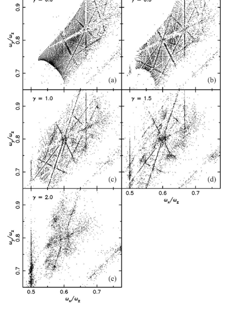
Figure 26: As in Fig.25 for the Dehnen (or $\gamma$) model Eq.(84), for various values of the parameter $\gamma$. Chaos becomes more prominent as the parameter $\gamma$ increases (after Valluri and Merritt 1998).

In these diagrams, areas filled with well ordered points correspond to regular orbits, whereas areas with scattered points correspond to chaotic orbits. We also distinguish various resonance lines and resonance strips with borders covered by chaotic orbits. A resonance line is specified by a linear combination of the form $k_{1}a_{1}+k_{2}a_{2}+k_{3}=0$ with integer $k_{1},k_{2},k_{3}$. At the intersection of two resonance lines there are periodic orbits of various stability types. Inside each resonance strip, on the other hand, there are invariant tori of dimensionality lower than three. The orbits near the central resonance lines are usually on 2D elliptic tori, which cause a concentration of points along the resonant line. On the other hand, the orbits in resonance lines devoid of points are usually on tori which are at least partially hyperbolic. The study of Papaphilippou and Laskar demonstrated in a clear way the complexity of the phase space in 3D galactic systems by giving detailed information not only about the existence of periodic orbits but also about the interaction of resonances. They also confirmed that triaxial systems with a flat central density profile contain all the types of regular orbits found in the simple perfect ellipsoid model (see Fig.24), but also many chaotic orbits that appear to play an important role in the system’s global dynamics.

Figure 27: As in Fig.26, for $\gamma=0.5$ and various mass values of a central black hole. The chaos in these cases is even more prominent than in the cases of Fig.26 (after Valluri and Merritt 1998).

Wachlin and Ferraz-Mello (1998) and Valluri and Merritt (1998) used the same technique as Papaphillippou and Laskar (1998) in order to study the dynamics of triaxial galaxies with cuspy central density profiles and massive black holes. These studies use the Dehnen (or $\gamma$) density model (Dehnen 1993, Tremaine et al. 1994)

$$\varrho(m)=\frac{(3-\gamma)M}{4\pi abc}m^{-\gamma}(1+m)^{-(4-\gamma)}$$ (84)

where $m^{2}=\frac{x^{2}}{a^{2}}+\frac{y^{2}}{b^{2}}+\frac{z^{2}}{c^{2}}$ with $a>b>c$. The total mass of the system is given by $M$ and the equidensity surfaces are stratified ellipsoids with axial ratio $a:b:c$. The parameter $\gamma$ specifies the form of the central density profile and can take values $0\leq\gamma<3$. For $\gamma=0$ we have a flat central density profile, while for $\gamma>0$ we have a cuspy profile, with $\rho\rightarrow\infty$ as $m\rightarrow 0$, and $\gamma$ regulating the logarithmic slope of the density profile. The studied values of $\gamma$ were $0\leq\gamma\leq 2$. Fig.26 shows the frequency maps in the domain of box orbits for different values of $\gamma$. These diagrams render obvious that, as the value of $\gamma$ increases, the total volume occupied by regular orbits decreases while that of chaotic orbits increases. Furthermore, the density of points near resonance lines increases. When $\gamma$ is large, the orbits near resonances are the only surviving regular orbits of the system.

Valluri and Merritt (1998) studied the case with $\gamma=0.5$ combined with massive central black holes. They found that chaos becomes even more prominent at the presence of the black hole, leading to full stochasticity when the mass of the black hole becomes of order $M_{h}\approx 0.03M_{galaxy}$ (Fig.27). The same authors noticed that the regular character of tube orbits is not greatly affected by the presence of a black hole or CMC, since, by definition, these orbits avoid anyway the center of the system.

4.6 Self-Consistent Models - Schwarzschild’s Method

The next step after a study of global dynamics is to examine the relative contribution of various types of orbits in supporting self-consistently the equilibrium state of the considered galactic model. The basic method towards such a study was introduced in stellar dynamics by M. Schwarzschild (1979). The main steps of Schwarzschild’s method are the following:

1) a spatial density function $\rho(\mathbf{r})$ is initially selected and we pose the question whether this function can represent the density of a galaxy in steady-state equilibrium. Via Poisson’s equation, the potential $\Phi(\mathbf{r})$ corresponding to $\rho(\mathbf{r})$ is obtained.

2) A grid of initial conditions is specified in a properly chosen subset of the phase space, e.g. on equipotential surfaces. The orbits with these initial conditions are integrated for sufficiently long time intervals. This creates a ‘library of orbits’ (typical number is of order $10^{4}$ orbits).

3) The configuration space is divided into small cells, and the time is recorded that each orbit spends inside each cell. Let $N_{c}$ be the number of cells, $N_{o}$ the number of orbits $(N_{c}<<N_{o})$ and $t_{oc}$ the time that the orbit $o$ spends inside the cell $c$. We then assign statistical weights $w_{o}$ $(o=1,...,N_{o})$ to the orbits that represent the relative contribution of each orbit, i.e., percentage of stars that follow the same orbit, in the system. Based on these weights, it is possible to construct a response density, that is the density in ordinary space created by the superposition of the orbits with the above weights. The problem is then to find for which values of the weights the response density can be made to match the imposed density, namely $\rho(\mathbf{r})$. Mathematically, we look for solutions for $w_{o}$ of

$$\sum_{i=1}^{N_{o}}w_{o}t_{oc}=m_{c}\quad c=1,...,N_{c}$$ (85)

where $m_{c}$ is the total mass in the $c$-th cell determined by the value of the imposed density $\rho(\mathbf{r_{c}})$ at the center $\mathbf{r_{c}}$ of the cell times the volume of the cell. We furthermore impose the constraint $w_{o}\geq 0$, since the density contributed by each orbit can only be a positive quantity.

In most implementations of the above algorithm, a solution to Eq.(85), under the imposed constraints, is seeked by reformulating the problem as an optimization problem. Namely, we look for weights that minimize the absolute difference, for all $c$, of the left and right hand sides of Eq.(85). This request takes the form of an objective function that is to be minimized. The problem is then solved by various algorithmic techniques such as linear programming solved e.g. by the Simplex method (see e.g. Schwarzschild 1979, Richstone and Tremaine 1984, Statler 1987), Non Negative Least Squares NNLS, (e.g. Pfenniger 1984, Wozniak and Pfenniger 1997, Rix et al. 1997), Lucy algorithm (e.g. Lucy 1974, Newton and Binney 1984, Statler 1987), maximization of a suitably defined ‘entropy’ functional (e.g. Richstone 1987) and Quadratic Programming (e.g. Merritt and Fridman 1996).

The main drawback in the above method is that the algorithm usually yields non-unique solutions. This is not physically unacceptable, since it is known that there can be more than one distribution functions compatible with a particular density function (Pfenniger 1984). However, the non-uniqueness of Schwarzschild’s solutions is also partly due to numerical reasons or to the fact that the problem’s formulation is not sufficiently constrained. This means that the number of unknowns in the equations (i.e. the weights) is larger than the number of available equations. This is because in Schwarzschild’s method we seek to match the distribution of matter only in configuration space but we ignore the velocity distribution which is an outcome of the method for any particular solution ${w_{o}}$. Thus, different solutions imply the same distribution in ordinary space but quite different distributions in velocity space. An alternative version of Schwarzschild’s method has been applied (Cretton et al. 1999, 2000) that requests, besides the spatial density, to reproduce also the velocity profiles observed along the line of sight (subsection 2.2). This new request reduces the number of solutions by increasing the number of equations, yet it still leaves some possibility for more than one solutions.

Another selection criterion among different solutions is the stability properties of each solution. Actually this is also a drawback of Schwarzschild’s method, since the latter cannot decide on whether a particular solution found by the method is stable or not. This can only be decided after an N-Body realization of the system is prepared and runs in the computer. Such a stability analysis for the original Schwarzschild (1979) model (Smith and Miller 1982) demonstrated that, despite the authors characterization of the model as ‘robust’, the model was actually not remaining in steady-state (see also Siopis 1999, p.80). This can be due to two reasons: a) the self-consistent fitting is not perfect, i.e., we find weights that minimize the difference between the imposed and response density, but the difference is not actually equal to zero, and b) the model found is not stable. Smith and Miller (1982) concluded that while the N-Body system was evolving in time, the differences in time were seemingly not growing exponentially.

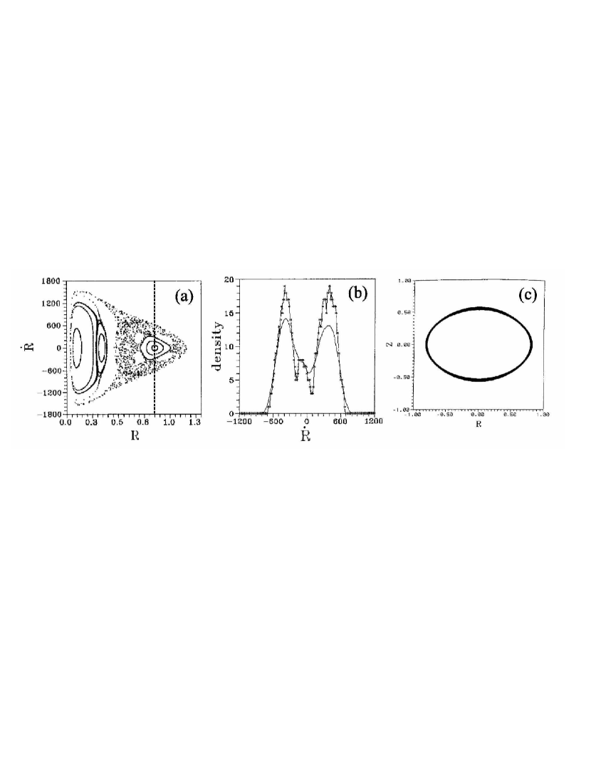
Figure 28: (a) Same as in Fig.7a. (b) The density of real particles of the N-Body system along a vertical line passing from the center of the 1:1 resonance (dashed line in (a)) has a minimum at the center of the resonance. (c) The form of a very thin tube orbit in the meridional plane around the stable 1:1 periodic orbit. The orbit is elongated perpendicularly to the Z-axis, while the system as a whole is elongated along the Z-axis (Fig.4).

For most other self-consistent models of galaxies presented so far in the literature, there have been no accompanying N-Body tests of the stability of the models. We believe, however, that such tests are indispensable, otherwise the conclusions drawn by the self-consistent modelling alone may not reflect real properties of the systems under study.

We finally mention a variant of Schwarzschild’s method implemented in disk galaxies, i.e., spiral (Contopoulos and Grosbøl 1986, Patsis et al. 1991), or barred (Kaufmann and Contopoulos 1996). In these authors’ approach, one has first to calculate the basic families of periodic orbits that (presumably) constitute the backbone of the galaxy. Then, one builds the library of orbits by considering initial conditions preferably in the neighborhood of the periodic orbits (e.g. with a Gaussian distribution). This method can be advantageous over Schwarzschild’s method in that one starts with some insight as regards which orbits play the major role in the galaxy, rather than using a blind grid of initial conditions. On the other hand, this can also turn to be a disadvantage in case the leading hypothesis about which orbits are important is wrong.

A further complication is due to the fact that there are cases in which the distribution of matter has a minimum rather than maximum near some particular stable periodic orbits. Such an example is shown in Fig.28, referring to the same N-Body experiment as in Figs.(4-7). In Fig.28a we see that, for a particular value of the energy, there is a large island of stability near a 1:1 stable periodic orbit of the system. If, however, we find the number of N-Body particles as a function of the distance from the central periodic orbit (Fig.28b), this plot has a minimum rather than maximum at the position of the periodic orbit. This is because the form of this orbit is an elongated ellipse (Fig.28c), but the elongation is at right angle with the elongation of the galaxy (Fig.4a,b). This means that the distribution of matter has to have a minimum near the particular periodic orbit, because the shape of this orbit, and of other nearby quasi-periodic orbits, cannot support the shape of the galaxy.

4.7 The importance of chaos through self-consistent models of galaxies

Schwarzschild (1979) constructed self-consistent models of triaxial elliptical galaxies using only regular orbits (box and SAT). In the decade following his paper, Schwarzschild’s method was implemented for the construction of self-consistent models using almost exclusively regular orbits (Schwarzschild 1982, Richstone 1980, 1982, 1984, Richstone and Tremaine 1984, Levison and Richstone 1987, Stattler 1987). These systems were either integrable (e.g. spherical or the perfect ellipsoid), or nearly-integrable (e.g. axisymmetric with a flat central density profile). Goodman and Schwarzschild (1981) pointed out that a large number of the orbits that were considered as regular in their models were in reality weakly chaotic (called ‘semistochastic’). However, these orbits exhibited a nearly regular behavior for times comparable to the galaxy’s lifetime. This means that the orbits obey an approximate integral of motion (subsection 2.3.2), or that they exhibit the ‘stickiness phenomenon’ (subsection 2.3) associated with slow Arnold diffusion in phase space.

On the other hand, as we have seen above, Schwarzschild (1993) searched for self-consistent solutions of cuspy halo models of the form $\varrho\propto r^{-2}$ near the center. In these models, he found a large number of chaotic orbits. For systems with a moderate ellipticity (smaller than E5), it was in fact possible to find multiple solutions that contained either a mixed population of regular and chaotic orbits or only regular orbits. But for more elongated models (ellipticities larger than E5) it was not possible to find any solution composed entirely by regular orbits. It thus became evident that cuspy models of elliptical galaxies render necessary the presence of chaotic orbits.

Merritt and Fridman (1996) studied the construction of self-consistent models in systems with the potential function corresponding to the $\gamma$ model for the values $\gamma=1$ (weak cusp) and $\gamma=2$ (strong cusp). In both models the axial ratios were $c/a=0.5$ and $b/a=0.79$. These correspond to a case of a maximally triaxial E5 galaxy, i.e. a galaxy with triaxiality

$$T=\frac{a^{2}-b^{2}}{a^{2}-c^{2}}$$ (86)

equal to $T\simeq 0.5$ (T=0 in oblate systems ($a=b$), and T=1 in prolate ($b=c$) systems). Furthermore, the same authors quantified the distinction of orbits into regular or chaotic by means of the Lyapunov characteristic number. They concluded that efforts to construct self-consistent models without the presence of chaotic orbits were unsuccessful in both cases of weak or strong cusps. If instead chaotic orbits are included in the same manner as regular ones (one weight assigned to each chaotic orbit), then it becomes possible to find successful models. In fact, these models are not precisely stationary, because the chaotic orbits exhibit observable diffusion in phase space, especially at low energy levels (where diffusion times are much smaller than the Hubble time). As a result, the superposition of orbits creates a model that changes shape in time. Furthermore, many chaotic orbits do not manage to fill ergodically the whole available connected chaotic domain during an integration time $\approx 100T_{dyn}$, which corresponds to the age of the system. Nevertheless, by ignoring chaotic orbits at low energy levels (which are responsible for the fastest diffusion), it was possible to produce quasi-stationary solutions that provided good self-consistent models, especially in the case of weak cusp.

The next step in the same study was the search of fully mixed solutions. These are solutions in which all the chaotic orbits of the library that correspond to the same value of the energy can essentially be considered as different pieces of only one orbit. If this can be established, the library representatives of this one orbit do not cause a macroscopic change in the shape of the response density field due to chaotic diffusion. This means that the resulting models are guaranteed to be stationary. Merritt and Fridman (1996) concentrated on such solutions applicable to the chaotic orbits of low energy levels. This was completely successful in the case of weak cusps, but only partly successful in the case of strong cusps. The so found ‘fully mixed’ solutions yielded large percentages of chaotic orbits in the final orbital composition, up to 45% in the case of weak cusps, and 60% in the case of strong cusps.

5 The N-Body approach

5.1 Numerical integration of the N-Body problem

The simplest method to integrate the N-Body problem, with $N$ large, is the so-called direct method, namely the direct numerical solution of the softened equations of motion

$$\mathbf{\ddot{r}_{i}}=-\sum_{j=1,j\neq i}^{N}{Gm_{j}(\mathbf{r_{i}}-\mathbf{r_{j}})\over\big{(}|\mathbf{r_{i}}-\mathbf{r_{j}}|^{2}+\epsilon^{2})^{3/2}}$$ (87)

for each particle $i=1,\ldots,N$. The softening parameter $\epsilon$ is introduced in order to avoid the singular behavior of the Keplerian force whenever two particles have a close approach. The value of $\epsilon$ should be such that the equations (87) ‘mimic’ the collisionless character of the system under study (subsection 2.1), without, however, introducing a large error to Newton’s law. Typical values are a fraction of $D/N^{1/3}$, where $D$ is the typical scale length of the integrated system. Specialized softening techniques are often combined with numerical implementations of regularization techniques (in the case of two-body encounters) or approximate regularization (for triple encounters). A review of these techniques is made by Aarseth (1994), a leading scientist in this field over decades.

The direct method is very accurate, but its algorithmic complexity is $O(N^{2})$, hence prohibitive for $N$ large. For this reason, Aarseth has developed codes that use a direct summation only for neighboring particles, while they use a multipole expansion of the potential, or the force, for groups of distant particles. The algorithm used to split the particles into neighboring or distant was introduced by Ahmad and Cohen (1973). The introduction of this scheme reduces the algorithmic complexity from $O(N^{2})$ to about $O(N^{1.5})$.

Another direction followed in order to reduce the computational cost of N-Body calculations was the construction of special hardware (GRAPE, e.g. Sugimoto et al. 1990, Makino and Funato 1993, Makino et al. 1997) based on specially designed chips to perform the sum (87) with speed exceeding by orders of magnitude any program written in conventional programming languages.

In simulations of galactic systems we are usually not interested in having an accuracy comparable to that requested in Celestial Mechanics. In the latter case the integration must often extend over billions of periods of the solar system bodies, while in the former case we are interested in integration times of order $10^{2}-10^{3}$ periods of the stars. Furthermore, in galactic dynamics we usually pose questions regarding the collective behavior of the system, which do not require an accuracy of integration of individual orbits as high as celestial mechanical calculations.

Such differences have led to the consideration of special techniques to integrate the N-Body problem with N large. Besides traditional ‘particles-in-cell’ or ‘grid’ methods (see the review by Sellwood 1987) that are applicable also to plasma physics, there are two methods that fit particularly the nature of the gravitational N-Body problem: the TREE method (Barnes and Hut 1986, Hernquist 1987, McMillan and Aarseth 1993), and the smooth potential field method (Clutton-Brock 1972, 1973, Allen et al. 1990, Hernquist and Ostriker 1992, Weinberg 1999). The so-called ‘spherical harmonics’ method (Villumsen 1982, McGlynn 1984, Merritt and Aguilar 1985) is a hybrid method similar to the smooth field code but with a ‘stepwise’ numerical calculation of the radial part of the spherical harmonics expansion of the potential of the system (Sellwood 1987), that requires sorting of the parcles with respect to their distances from the center. There have also been simulations in which the collisionless Boltzmann equation (16) is solved directly. This is numerically tractable in systems forced to retain a particular symmetry (usually spherical). The Boltzmann equation can be integrated either through calculation of its moments (e.g. Hoffman et al. 1979), or by its characteristic system of ordinary differential equations (e.g. Hénon 1964, Burkert 1990, Henriksen and Widrow 1997).

The main idea of the TREE algorithm (Barnes and Hut 1986) is to define a criterion by which, considering, say, the i-th particle of the system, the other particles can be divided in groups of close or distant particles with respect to the position of the i-th particle. The forces on i-th particle by close particles are added by direct summation. However, the forces of distant particles are added by considering one term for each group rather than for each particle. This effectively reduces the algorithmic complexity of the code from $O(N^{2})$ to $O(N\log N)$.

In the algorithm of Barnes and Hut (1986) all the particles are set initially in one cubic cell of volume $s_{0}$. This cell is divided by consecutive bisections into subcells of volume $s_{k}=s_{0}/2^{3k}$, where the index $k=1,2,\ldots$ denotes the order of division. If, for some order $k$, one subcell contains no more than one particle, this subcell is not further divided, otherwise the subdivision continues at order $k+1$. The data structure storing the hierarchy of all subcells is called the ‘tree’.

A ‘tolerance parameter’ $\theta_{tol}$ is also defined in to distinguish close cells from distant cells with respect to the position of one particle (suggested values are around $\theta_{tol}\approx 1$, Hernquist 1987). Considering the i-th particle, a cell is called distant if the following condition holds:

$$r\geq{s_{k}^{1/3}\over\theta_{tol}}$$ (88)

where $r$ is the distance of the cell from the i-th particle. If condition (88) is true, the particles in the cell are viewed as one group of mass $M_{c}$ (the sum of the particles’ masses). The contribution of this group to the force on the i-th particle is calculated by a multipole expansion (usually up to quadrupole terms).

The TREE method is very efficient. While the integration time is drastically reduced, there are many different cases of N-Body experiments that can be effectively treated with TREE. Examples are a) collapsing galaxies (e.g. Cannizzo and Holister 1992, Curir et al. 1993, Voglis 1994a, Voglis et al. 1995) b) merging galaxies (Barnes 1988, 1992, Hernquist 1992, Viturro and Carpintero 2000, Burkert and Naab 2003), c) multiple merger events (Efthymiopoulos and Voglis 2001), and d) Cosmological simulations (where TREE is often combined with a particle-mesh (PM) algorithm, Bouchet and Hernquist 1988, Kravtsov et al. 1997). This flexibility is due to the fact that the TREE code can follow simultaneously the evolution of different parts of a system that may have large density contrasts or a rapidly varying spatial distribution. For these reasons, TREE codes or hybrid TREE - PM codes have been developed continually over the years, resulting in drastic improvements of the $O(N\log N)$ scaling (e.g. Dehnen 2000) and in parallel implementations of the algorithm for either galactic or cosmological simulations (e.g. Warren and Salmon 1993, Dubinski 1996, Kravtsov et al. 1997, Viturro and Carpintero 2000, Springel et al. 2001, Becciani and Antonuccio-Delogu 2001, Miocchi and Capuzzo-Dolcetta 2002, Bode and Ostriker 2003). The TREE code can also be combined with the special hardware GRAPE (e.g. Fukushige et al. 1991, Athanassoula et al. 1998).

On the other hand, the main disadvantage of the TREE code is that it does not allow one to have the potential function of the system $\Phi(\mathbf{x},t)$ in a closed analytical form. This means that one cannot make global dynamical studies with TREE, such as, e.g., the calculation of orbits, variational equations, Poincaré sections, frequency maps etc. (section 4).

The class of self-consistent field codes is particularly suited to global dynamical studies of galaxies. The main idea in such codes is that a spatial distribution of particles represents a Monte Carlo realization of an ideally smooth density field. The smooth density $\rho$ is given by Eq.(6), i.e., in terms of a smooth distribution function $f$. If the system’s geometry is not very peculiar, the smooth function $\rho(\mathbf{x})$ can be expanded in a truncated series of basis functions. Different basis functions can be chosen taylored to the particular properties of the system under study.

We shall follow the formalism of Weinberg (1999) in order to show the method to obtain suitable sets of basis functions for triaxial systems. If we anticipate that the average density profile of the system that is to be simulated will not be very different from a model function $\rho_{00}(r)$, we express the monopole term of the density as a truncated series of the form:

$$\rho_{monopole}(r)=\rho_{00}(r)\sum_{n=0}^{n_{max}}b_{n00}u_{n00}(r)$$ (89)

The sum in the r.h.s. represents the residuals of the fit of the monopole term of the real density of the system by the model density $\rho_{00}(r)$. The coefficients $b_{n00}$ are unknown and the main task of the N-body code is to find their values. The functions $u_{n00}(r)$, on the other hand, are known functions which are eigenfunctions of a Sturm-Liouville problem specified below. We can similarly express all multipole contributions to the density, i.e., we fix some model functions $\rho_{ml}(r)$ and express the density as:

$$\rho(r,\theta,\phi)=\sum_{l=0}^{l_{max}}\sum_{m=-l}^{l}\sum_{n=0}^{n_{max}}b_{nml}\rho_{ml}(r)u_{nml}(r)Y_{l}^{m}(\theta,\phi)$$ (90)

with functions $u_{nml}(r)$ specified by a Sturm-Liouville problem and coefficients $b_{nml}$ calculated by the N-Body code.

The Sturm-Liouville problem for $u_{nml}(r)$ is formulated as follows: writing the potential in a form similar to (90)

$$\Phi(r,\theta,\phi)=\sum_{l=0}^{l_{max}}\sum_{m=-l}^{l}\sum_{n=0}^{n_{max}}c_{nml}\Phi_{ml}(r)u_{nml}(r)Y_{l}^{m}(\theta,\phi)$$ (91)

we couple equations (90) and (91) via Poisson equation (7) in spherical coordinates. After the separation of variables, this leads to:

$$-\dfrac{d}{dr}\left(r^{2}\Phi_{ml}^{2}\dfrac{du_{nml}}{dr}\right)+\left[l(l+1)\Phi_{ml}^{2}-\Phi_{ml}\dfrac{d}{dr}\left(r^{2}\dfrac{d\Phi_{ml}}{dr}\right)\right]u_{nml}=\\ -(4\pi G\lambda_{nml}r^{2}\Phi_{ml}\rho_{ml})u_{nml}$$ (92)

with $\lambda_{nml}=b_{nml}/c_{nml}$. This equation, supplemented with appropriate boundary conditions at two particular radii $r_{a}$ and $r_{b}$ is a case of the Sturm-Liouville eigenvalue problem

$$-\dfrac{d}{dx}\left[p(x)\dfrac{dy}{dx}\right]+q(x)y=\lambda w(x)y$$ (93)

with

$$\begin{split}p(x)&=x^{2}\Phi_{ml}^{2}(x)\\ q(x)&=l(l+1)\Phi_{ml}^{2}(x)-\Phi_{ml}(x)\dfrac{d}{dx}\left(x^{2}\dfrac{d\Phi_{ml}(x)}{dx}\right)\\ w(x)&=-4\pi Gx^{2}\Phi_{ml}(x)\rho_{ml}(x)\end{split}$$ (94)

The functions $u_{nml}(r)$ are eigenfunctions of a differential operator acting on $u_{nml}$ in the l.h.s. of Eq.(92). Since this operator does not depend on $n$, the index $n$ can be identified to the serial index of successive eigenvalues and eigenvectors, starting from the ground state value $n=0$. The problem is well defined if boundary conditions are given in the form

$$\begin{split}a_{1}u-a_{2}\left(p(r)\dfrac{du}{dr}\right)&=\lambda\left(a_{1}^{\prime}u-a_{2}^{\prime}\dfrac{du}{dr}\right)\qquad\text{at}\quad r=r_{a}\\ b_{1}u+b_{2}\left(p(r)\dfrac{du}{dr}\right)&=0\qquad\qquad\qquad\quad\quad\quad\text{at}\quad r=r_{b}\end{split}$$ (95)

In galactic problems, the radii $r_{a},r_{b}$ are set equal to $r_{a}=0$ (center of the system), and $r_{b}=R_{p}$ or $r_{b}\rightarrow\infty$. If $r_{b}=R_{p}$, the radius $R_{p}$ is set to represent the size of the system, and the boundary conditions at $R_{p}$ are obtained by the request of continuity, and continuous derivative, of the potential function at the point $R_{p}$ where we pass from Poisson to Laplace equation.

If the model functions $\Phi_{ml}(r)$, $\rho_{ml}(r)$ satisfy Poisson’s equation, they are called potential - density pair functions. The eigenfunctions of the Sturm-Liouville problem (92) are mutually orthogonal with respect to the inner product definition:

$$<f|g>=\int_{r_{a}}^{r_{b}}f(r)g(r)w(r)dr$$ (96)

The above equations provide the general framework of the self-consistent field method. In order to have a concrete N-body implementation we proceed by the following steps:

a) Specify a set of potential - density model functions $\Phi_{ml}(r)$, $\rho_{ml}(r)$. These are arbitrary functions which may, or may not really depend on the indices $l$, or $m$.

b) Substitute the functions $\Phi_{ml}(r)$ and $\rho_{ml}(r)$ in Eq.(92) and solve the Sturm-Liouville problem. This will specify the eigenfunctions $u_{nml}$ and eigenvalues $\lambda_{nml}$. Although a numerical solution of Eq.(92) is in principle possible for any choice of $\Phi_{ml}(r),\rho_{ml}(r)$, we prefer to use sets of functions for which the solution of Eq.(92) is reduced to known functions from the literature. Examples are:

- the Clutton-Brock (1973) set:

$$\begin{split}\rho_{ml}(r)&=\sqrt{4\pi}\dfrac{r^{l}}{(1+r^{2})^{l+5/2}}\\ \Phi_{ml}(r)&=-\sqrt{4\pi}\dfrac{r^{l}}{(1+r^{2})^{l+1/2}}\end{split}$$ (97)

in which the eigenfunctions $u_{nlm}(r)$ are Gegenbauer polynomials of the form $C_{n}^{l+1}(\xi)$ where $\xi=\frac{r^{2}-1}{r^{2}+1}$,

- the set of Allen et al. (1990)

$$\begin{split}\rho_{ml}(r)&=-1\\ \Phi_{ml}(r)&=1\end{split}$$ (98)

where the eigenfunctions $u_{nml}(r)$ are spherical Bessel functions, and

- the Hernquist - Ostriker (1992) set

$$\begin{split}\rho_{ml}(r)&=\sqrt{4\pi}\dfrac{1}{2\pi}\dfrac{(2l+1)(l+1)}{r}\dfrac{r^{l}}{(1+r)^{2l+3}}\\ \Phi_{ml}(r)&=-\sqrt{4\pi}\dfrac{r^{l}}{(1+r)^{2l+1}}\end{split}$$ (99)

where the eigenfunctions $u_{nml}$ are Gegenbauer polynomials of the form $C_{n}^{2l+\frac{3}{2}}(\xi)$ where $\xi=\frac{r-1}{r+1}$.

In the case of galactic disks, potential-density pairs were proposed by Clutton-Brock (1972), Kalnajs (1976), Aoki and Iye (1978) and Earn (1996). We note that such pairs are also extremely useful in the study of the stability properties of galaxies (e.g. Palmer 1995).

c) Given the positions of the $N$ particles, we calculate the coefficients $b_{nml}$ and $c_{nml}$ of the full density and potential expansions (90) and (91). We determine first the coefficients $b_{nml}$ by exploiting the orthogonality of the functions $u_{nml}$, i.e. $<u_{nml}|u_{n^{\prime}ml}>=\delta_{n,n^{\prime}}$, as well as the orthogonality of the spherical harmonic functions. If we multiply both sides of Eq.(90) by $w(r)u_{nml}(r)Y_{l}^{m}(\theta,\phi)$ and take the integral over all positions we find:

$$b_{nml}=\int_{r_{a}}^{r_{b}}\int_{0}^{\pi}\int_{0}^{2\pi}w(r)\rho(r,\theta,\phi)u_{nml}(r)Y_{l}^{m*}(\theta,\phi)drd\theta d\phi$$ (100)

Assuming that the positions of the N particles provide a Monte Carlo sampling of the function $\rho(r,\theta,\phi)$, the triple integral in (100) can be approximated by a sum over particles:

$$b_{nml}\simeq\sum_{i=1}^{N}w(r_{i})u_{nml}(r_{i})Y_{l}^{m*}(\theta_{i},\phi_{i})$$ (101)

The potential coefficients $c_{nml}$ are finally determined via the relation $c_{nml}=b_{nml}/\lambda_{nml}$.

The use of the Monte Carlo integration method implies that, contrary to what the term ‘smooth field’ might signify, there is some sort of noise in the system introduced by its discreteness. This noise appears in a quite different way than in the direct or TREE algorithm. Namely, the uncertainties, or inevitable small fluctuations of the coefficients $b_{nml}$ during the simulation of even an ‘equilibrium’ system result in a relaxation of this system which is essentially due to discreteness effects (see Weinberg 1998 for a detailed discussion). However, this noise is reduced, in general, as the number of particles $N$ increases. As $N$ increases we may also use a larger number of basis functions to fit the density, or the potential.

Since the calculation of the sum (101) has an $O(N)$ algorithmic complexity, the overall complexity of a smooth field code scales linearly with $N$. This, in combination with the fact the parallelization of the sum (101) is straightforward, renders such codes very powerful even in small computers or computer clusters, with applications reaching $N=10^{7}-10^{8}$.

Besides its linear algorithmic complexity, the main power of a smooth field code lies in that the outcome of the potential evaluation can be expressed analytically in terms of a series of basis functions. This allows one to have the Hamiltonian of the system in closed form, a fact which greatly facilitates the orbital or global dynamical study of the system. The use of smooth field codes has been very fruitful in galactic dynamics so far, and we can anticipate only better prospects for the future.

5.2 The Global Dynamics of N-Body systems

We have already discussed Schwarzschild’s method for the construction of self-consistent models of galaxies as well as the limitations of this method (subsection 4.5). Such limitations are not present if one uses N-body simulations. The equilibria of such simulations are by definition self-consistent and stable. Thus, questions like what is the relative importance of ordered or chaotic orbits in a galaxy are better answered within the framework of global dynamical studies of N-Body systems. The N-Body method allows one to deal also with systems exhibiting secular evolution such as, e.g., systems with a CMC or central black hole.

An early example of orbital analysis in triaxial systems resulting from N-Body simulations was given by Udry and Martinet (1994). These authors presented histograms yielding the distribution of particles with respect to the ratios of the fundamental frequencies of their orbits. They subsequently discuss the link between the orbital structure and the shape of the N-Body systems.

A extended study of global dynamics in N-Body systems was made by Voglis et al. (2002), Kalapotharakos et al. (2004) and Kalapotharakos and Voglis (2005). This is a study of N-Body systems in equilibrium resulting from the cosmological simulations described in subsection 2.5. We have seen that spherically symmetric (or ‘quiet’) initial conditions lead to very elongated galaxies as a result of the radial orbit instability. We call such an experiment the ‘Q-system’. On the other hand, clumpy initial conditions lead to a less elongated final state (the ‘C-system’). These systems remain in a steady state for long time periods ($>>1t_{Hubble}$). The smooth field code of Allen et al. (1990) is used to calculate a smooth analytic potential and the corresponding density. These are given by:

$$\Phi(r,\vartheta,\varphi)=-\frac{G}{R_{0}}\sum_{l=0}^{\infty}\sum_{n=0}^{\infty}\sum_{m=-n}^{n}b_{lmn}j_{n}\left(a_{ln}\frac{r}{R_{0}}\right)P_{n}^{|m|}(\cos\vartheta)e^{im\varphi}~{}~{}~{}\mbox{if}~{}~{}~{}r\leq R_{0}$$ (102)

$$\Phi(r,\vartheta,\varphi)=-\frac{G}{R_{0}}\sum_{l=0}^{\infty}\sum_{n=0}^{\infty}\sum_{m=-n}^{n}b_{lmn}j_{n}\left(a_{ln}\right)\left(\frac{R_{0}}{r}\right)^{n+1}P_{n}^{|m|}(\cos\vartheta)e^{im\varphi}~{}~{}~{}\mbox{if}~{}~{}~{}r>R_{0}$$ (103)

$$\rho(r,\vartheta,\varphi)=\frac{1}{4\pi R_{0}^{3}}\sum_{l=0}^{\infty}\sum_{n=0}^{\infty}\sum_{m=-n}^{n}a^{2}_{ln}b_{lmn}j_{n}\left(a_{ln}\frac{r}{R_{0}}\right)P_{n}^{|m|}(\cos\vartheta)e^{im\varphi}~{}~{}~{}\mbox{if}~{}~{}~{}r\leq R_{0}$$ (104)

where $b_{lmn}$ are the coefficients of the expansion and $R_{0}$ is a parameter of the code fixing the outermost radius inside which Poisson’s equation is solved. The functions $j_{n}(r)$ are spherical Bessel functions and $P_{n}^{m}$ are Legendre polynomials.

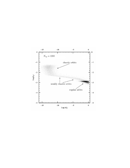
Figure 29: The distinction of regular and chaotic orbits on the $(\log L_{j}-\log AI_{j})$ plane. The orbits with small values of $AI_{j}$ and stabilized values of $L_{j}$ are identified as chaotic orbits. The orbits with large values of $AI_{j}$ ($>10^{-3}$) and decreasing values of $L_{j}$ (as $t^{-1}$) are identified as regular orbits. The orbits on the lane joining the two regions are weakly chaotic orbits (after Voglis et al. 2002).

When calculating orbits, care is needed as regards the characterization of an orbit as regular or chaotic. The usual criterion of the Lyapunov characteristic number

$$LCN=\lim_{t\rightarrow\infty}{1\over t}\ln\left|{\xi(t)\over\xi(0)}\right|$$ (105)

cannot be applied in a straightforward manner in the case of galaxies. The reason has to do with the (inevitably) finite time of numerical integration of orbits (in order to obtain an estimate of the LCN), that has to be compared with the lifetime of the system. In fact, the periods of stars in the inner and outer parts of a galaxy differ by about three orders of magnitude. This suggests that the Lyapunov times of orbits (inverse of the LCNs) be normalized with respect to the periods of orbits. On the other hand, the lifetime of the galaxy defines a second relevant timescale, i.e., an orbit is effectively chaotic only if its Lyapunov time is of the order of the galaxy’s lifetime or smaller. This second timescale is uniform for all orbits. The question then is what is a proper normalization of Lyapunov times (or Lyapunov exponents) that provides a fair measure of the ‘chaoticity’ of an orbit.

In order to address this question, Voglis et al. (2002) introduced a new type of calculation based on the combination of two methods: a) the ‘specific time Lyapunov number’ $L_{j}$, normalized with respect to the orbit’s inverse of the period, and b) the Alignment Index (AI). The Alignment Index is a numerical method based on certain properties of the time evolution of deviation vectors (Voglis et al., 1998, 1999, Skokos, 2001). Along regular orbits the index AI has a value close to unity while along chaotic orbits it tends exponentially to zero.

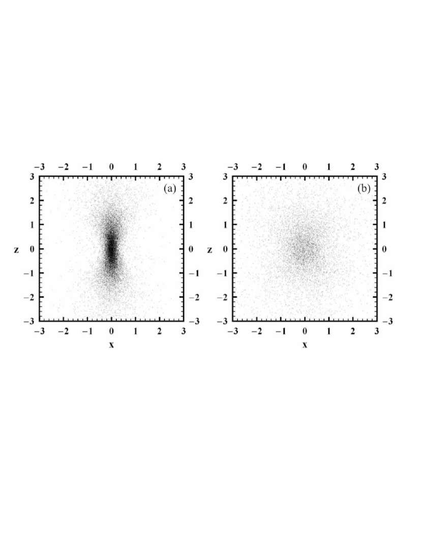
Figure 30: , Projection of the particles in (a) regular and (b) chaotic orbits on the plane of short - long axis. The distribution of chaotic orbits is almost spherical while the distribution of regular orbits is strongly elongated along the long axis of the system. (after Voglis et al. 2002).

In order to make the distinction of the orbits, one considers a particular snapshot of the system and uses the potential expansion (102-103) as a time-independent potential in which orbits can be calculated. The orbits with initial conditions given by the positions and velocities of the N-Body particles are integrated. The distinction of the orbits in the case of the Q system, after an integration for $N_{rp}=1200$ radial periods of each orbit, is shown in Fig.29. The triangular group of points in the down-right part of the diagram corresponds to regular orbits with $\log(AI)\gtrsim-3$ and Lyapunov numbers decreasing in time as $t^{-1}$. The group of points in the up-left part ($\log(AI)<-12$) are chaotic orbits. The index $AI$ of such orbits reaches, after a fast decrease, the accuracy limit of the computer. Furthermore, their calculation of the LCN stabilizes to a positive limit. We also distinguish a lane of points connecting the two groups. These are particles in weakly chaotic orbits. In this case the time evolution of the index $AI$ shows a relatively slow decrease, compared to that of strongly chaotic orbits.

Based on the above method, the bodies found in chaotic orbits are 23% and 32% of the total mass in the C and Q system respectively. When the whole procedure was repeated after 100 half-mass crossing times ($T_{hmct}$), the above percentages remained essentially unaltered. Keeping track of the identities of particles that where characterized in regular or chaotic orbits, there was no change of character except for a 3% of the particles.

It should be stressed that only a fraction of the particles characterized chaotic can, in fact, develop appreciable chaotic diffusion within a Hubble time. The estimated percentage of such particles is less than 8%. Although most orbits are only weakly chaotic, the spatial distribution of the chaotic mass component is very different from that of the regular component (Fig.30). Namely, the chaotic component is distributed rather spherically, i.e., isotropically, while the regular component has a spatial distribution elongated in the direction of the long axis of the system. Moreover, contrary to the regular component, the chaotic component has a flat central surface density profile (Fig.31). The superposition of the two profiles creates a hump in the total surface density profile roughly at the point where the two profiles cross each other. In the case of the Q-system, this transition is manifested also in the ellipticity profile (Fig.32) which has an abrupt decrease by two units from the inner region, where regular orbits dominate, to the outer region, where chaotic orbits dominate.

The conclusion is that there is an upper limit to the ellipticity of galaxies containing chaotic orbits, while systems with only regular orbits can reach much larger values of the ellipticity.

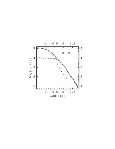
Figure 31: Profiles of the surface density on the projected plane of short - long axis for the regular component (dashed line), chaotic component (dotted line) and the overall system (solid line). The superposition of the two profiles (regular and chaotic) creates a hump in the overall surface density profile roughly at the point where the two partial profiles cross each other (after Voglis et al. 2002).

In a similar study, Muzzio et al. (2005) found that the fraction of mass in chaotic motion in their system (similar to the Q-system above) is about $53\%$. This larger fraction is due to two reasons: a) the use of a smaller threshold in the Lyapunov number for the characterization of an orbit as chaotic, and b) a less flat density profile near the center. However, the different spatial distribution of the particles in regular or chaotic orbits (as in Fig.30), was also found in the experiments of Muzzio et al.

There is a variety of different orbital structures that are able to support systems with smooth centers (Contopoulos et al. 2002, Kalapotharakos and Voglis 2005, Kalapotharakos 2005, see also Jesseit et al. 2005). This seems to apply both to regular and chaotic orbits. The self-consistency condition imposes some restrictions on the permissible orbital distributions. For example, the Q-system, being very elongated, is formed by particles moving almost exclusively in box orbits, and it has only a small fraction of particles in tube types (SAT or LAT). This, despite the fact that the SAT and LAT types of orbits are very stable and occupy an extended domain in phase space. On the other hand, in the C system, which is more spherical, the particles move preferentially in tube orbits, especially SAT. This fact clearly shows that even if a global dynamical analysis establishes the existence of large domains of stability in phase space, this does not imply that the real particles of the N-Body system will fill these domains. The preferential domains in phase-space are only partly determined by the regular or chaotic character of the orbits. The other determining factor is the request for self-consistency.

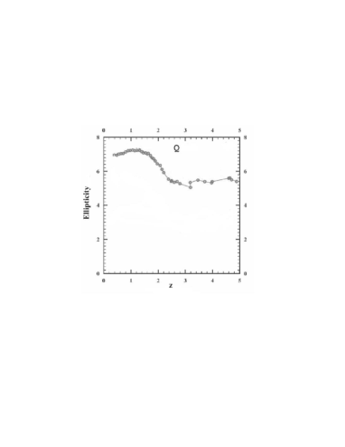
Figure 32: The ellipticity of the Q-system on the short-long axis plane as a function of the distance from the center along the long axis $z$. The abrupt decrease of the ellipticity at about $r_{rc}=2$ marks the transition from a region where regular orbits dominate (inside $r_{rc}$) to a region where chaotic orbit dominate (outside $r_{rc}$) (after Voglis et al. 2002).

Fig.33 shows the orbital content of the Q-system in frequency space (the fundamental frequencies are calculated by the algorithm of Sidlichovsky and Nesvorny 1997). The points correspond to particles moving on regular orbits (Fig.33a), and chaotic orbits (Fig.33b). In Fig.33a we can distinguish the distribution of particles in different domains of the frequency space, according to whether an orbit is of the box type or one of the tube subtypes. The points in Fig.33b show a scatter due to their chaotic character, which implies variability of the frequencies. The orbits with large variability of frequencies have also large Lyapunov characteristic numbers. Nevertheless, there are also chaotic orbits that remain localized along the resonance lines of other, regular, orbits. These are weakly chaotic orbits which are temporarily trapped in particular resonances, diffusing mostly along the resonance lines and only marginally across these lines.

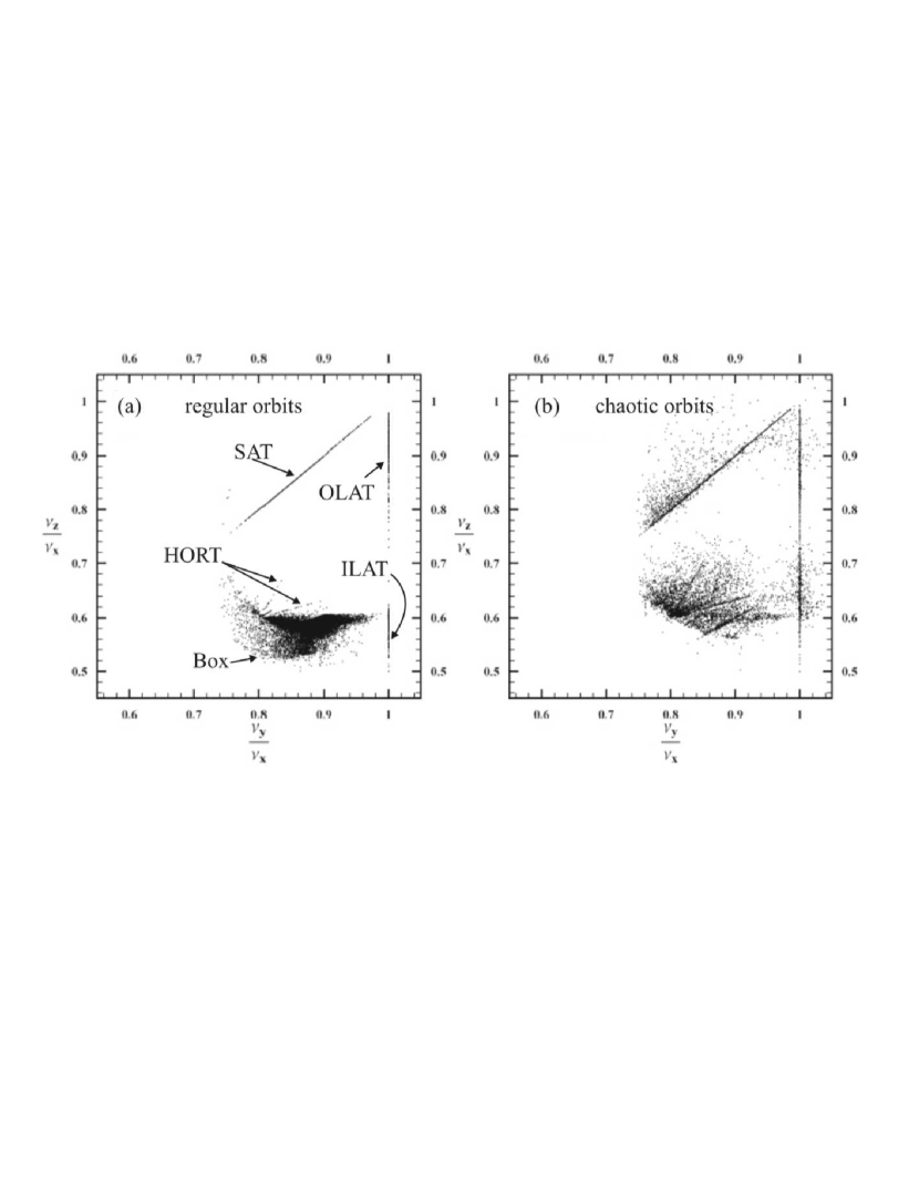
Figure 33: Frequency maps (rotation numbers) for (a) the regular and (b) the chaotic orbits of the Q-system. The regions of various types of regular orbits are marked in (a). In (b) many chaotic orbits are concentrated in particular resonance lines and they diffuse mainly along these lines (after Kalapotharakos and Voglis 2005).

5.3 Secular evolution under the presence of a CMC. Self-organization

Secularly evolving models can be created by inserting a black hole, or CMC, to a Q or C system (Kalapotharakos et al. 2004). The evolution and the properties of these systems depend on the value of the relative mass parameter $m=\frac{M_{cmc}}{M_{galaxy}}$. We consider values of $m$ in a range [0.0005, 0.01]. Just after the insertion of the CMC, the fraction of mass in chaotic motion increases suddenly to the level of 80% in systems generated by the Q-system, and 50% in systems generated by the C-system. The sudden rise of the chaotic component causes a secular evolution in these systems (subsection 4.6). This is mainly due to the anisotropic, i.e. non-mixed distribution of the chaotic orbits caused by the fact that, before the insertion of the CMC, these were mostly regular orbits (boxes) of the original system. Voglis and Kalapotharakos (2006) found that the mean rate of exponential divergence (or mean level of LCN) of this chaotic component has a narrow correlation with $m$, scaling as $m^{1/2}$. Furthermore, in order to measure the effectiveness of chaotic diffusion, these authors defined a parameter called ‘effective diffusion momentum’ ${\cal L}$ as the product of the anisotropically distributed chaotic mass times the mean logarithmic divergence of the orbits of this mass. Numerically, it is found that the parameter ${\cal L}$ measures the ability of secular evolution of the system. Namely, if ${\cal L}\lesssim 0.0045$ there is negligible secular evolution due to chaotic diffusion even for times longer than a Hubble time. On the other hand, if ${\cal L}\gtrsim 0.0045$ the models evolve following a process of self-organization that converts chaotic orbits to regular. The resulting reduction of entropy is partly balanced by the increase of the mean level of exponential divergence of the remaining chaotic orbits. During the whole process, the fraction of chaotic mass distributed anisotropically decreases in time, resulting in smaller values of ${\cal L}$. The evolution ceases when ${\cal L}$ goes below the value 0.0045.

Figure 34: The distribution of the real particles with respect to values of $\log L_{j}$ in four models with CMCs. For larger values of the mass $m$, the maximum of the distributions is shifted at larger values of $\log L_{j}$ (after Kalapotharakos et al. 2004).

Fig.34 shows the distributions of the Lyapunov numbers for all the systems after half a Hubble time from the CMC insertion. Smaller CMCs produce in general smaller Lyapunov numbers (the Lyapunov number at the peak of the distribution scales with $m$ as $m^{1/2}$). This also implies a slower rate of secular evolution. In fact, the morphology of systems with small CMCs ($m\leq 0.001$) remains close to the morphology of the original Q or C systems for at least a Hubble time, as indicated by a plot of the time evolution of the triaxiality index $T$ (Fig.35). The fact that regular orbits of the original systems are now characterized as weakly chaotic does not have serious consequences in the resulting morphology of the systems.

In systems with $m\geq 0.005$ the secular evolution is faster, and it leads from a prolate, or maximally triaxial shape to a final equilibrium which is characterized either by almost zero triaxiality (oblate), or moderate triaxiality, depending on the size of $m$ and on the initial orbital distribution of the system at the time when the CMC is inserted. Larger CMCs and small initial percentages of tube orbits (like in the Q-system) favor oblate final equilibria.

During the secular evolution of the systems, the fraction of mass in chaotic motion decreases in time, and in the final equilibrium it reaches a range 12% to 25%. As already mentioned, the systems present strong indications of self-organization. This means that in the course of secular evolution, many chaotic orbits are gradually converted into regular orbits of the SAT type. This process can be understood with the help of Figs.36 and 37. Figs.36a-d show projections of the 4D Poincaré sections at successive snapshots of the secular evolution of a Q-system with a CMC $m=0.01$. The phase portraits in the background are obtained by integrating many reference orbits in a potential frozen at the time corresponding to each snapshot. On the other hand, the orbits of the real particles of the N-Body system are integrated in an evolving N-Body potential and superposed on the phase portraits at different snapshots. Fig.36 shows the successive Poincaré consequents (stars or dots) of one orbit of a real particle. Initially, before the insertion of the CMC, this is box orbit. Thus, immediately after the insertion this orbit becomes a chaotic orbit yielding Poincaré consequents on the chaotic domain of the surface of section (stars). However, as the volume of the regular domain progressively increases, the character of the orbit is converted at a particular moment from chaotic to regular (open circles). The new regular orbit is of the SAT type. As a result of many such orbits, the triaxiality parameter $T$ of the system decreases.

Figure 35: The time evolution of the triaxiality parameter $T$ in various systems. One Hubble time corresponds to $t_{Hub}\approx 300$. The systems (Q, $m=0.01$), (Q, $m=0.005$) and (C, $m=0.01$) reach an oblate ($T=0$) final equilibrium state. Only the system (Q, $m=0.01$) achieves this equilibrium within a Hubble time. The (C, $m=0.005$) system reaches an equilibrium with modest triaxiality. Systems with smaller CMCs $(m\leq 0.001)$ do not appear to evolve significantly within a Hubble time (e.g. system (Q, $m=0.001$) (after Kalapotharakos et al. 2004).

Figure 36: Projections on the ($R,V_{R}$) plane of the 4D Poincaré section $z=0,\dot{z}>0$ at four different snapshots of the evolution of the (Q, $m=0.01$) system, at times a) $t=5$, b) $t=120$, c) $t=185$ and d) $t=355$. The island of stability to the right corresponds to SAT orbits and its size increases as a result of changes in the self-consistent potential. The stars or dots give the successive Poincaré consequents of an orbit which was a box in the original Q-system (before the insertion of the CMC), up to the time corresponding to each panel. A star is plotted as long as the orbit falls in the chaotic domain of the surface of section. part of the portrait. A dot is plotted after the moment when the orbit is captured in the regular domain (after Kalapotharakos et al. 2004).

Figs.37a-d show the particles of the Q-system (with $m=0.01$) on the plane of rotation numbers at four different snapshots ($t=30,90,150,210$, a Hubble time corresponds to 300 time units). Initially the box orbits of the original Q system are converted to chaotic orbits or they are trapped along the various resonance lines of HORT orbits. As the chaotic orbits diffuse in the phase space the system’s geometry changes. Namely, the system becomes less elongated and its triaxiality parameter $T$ decreases. Due to this evolution, some particles are trapped in orbits confined on SAT tori. During this self-consistent evolution the areas of HORT and ILAT orbits move upwards, approaching the line of SAT orbits. The number of SAT orbits increases while the number of all other orbital types decreases. At the equilibrium position there are only regular orbits of SAT type and chaotic orbits.

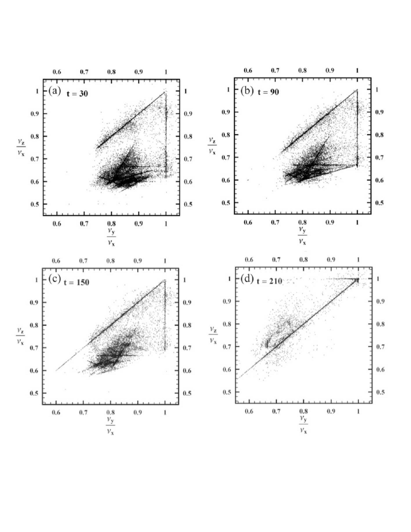
Figure 37: Frequency maps for the orbits of all the particles of the (Q, $m=0.01$) system at the snapshots a) $t=30$, b) $t=90$, c) $t=150$, and d) $t=210$. Initially there are many (previously box) chaotic orbits, trapped in various resonance lines (a). During the self-consistent evolution of the system, the population of SAT orbits increases while the population of all other types of orbits decreases (b,c). At equilibrium all orbits are either regular (of SAT type) or chaotic (d) (after Kalapotharakos and Voglis 2005).

Kalapotharakos et al. (2004) concluded that a system must have a CMC of at least $m\approx 0.01$, in order to complete its evolution and reach a new equilibrium state within a Hubble time. For smaller mass parameters the evolution to equilibrium is prolonged over many Hubble times. The exact evolution rate of the systems with CMCs depends mainly on two factors. a) the fraction of non-mixed chaotic orbits and b) the mean Lyapunov number of these orbits (Voglis and Kalapotharakos 2006). For example, the C-system with $m=0.01$ needs longer time than the Q-system with the same $m$ in order to evolve towards the final oblate configuration (Fig.35). This is because the C-System, as we have seen above, had initially a smaller fraction of box orbits than the Q-system. Therefore, after the insertion of the CMC, the C-system has a smaller fraction of chaotic orbits than the Q-system.

These results are in agreement with previous studies of Merritt and Quinlan (1998) and Holley-Bockelmann et al. (2002). Merritt and Quinlan (1998) studied the evolution of systems for various values of the mass of the central black hole. The black hole is inserted at the center of a maximally triaxial E5 elliptical galaxy in equilibrium. They found that black holes with $m=0.01$ are capable to make the system evolve towards an oblate axisymmetric configuration within a Hubble time. On the other hand, Holley-Bockelmann et al. (2002) found that the insertion of a black hole with mass $m=0.01$ leaved unchanged their system (especially in the external parts). However, the original system that they used was a triaxial E2 elliptical galaxy, while the original system of Merritt and Quinlan (1998) is similar to the Q-system considered above (many box orbits). As explained above, given that box orbits become chaotic after the insertion of the black hole, such a system evolves rapidly towards a new equilibrium. On the contrary, the system of Holley-Bockelmann et al. (2002) (similar to the C-system above) has a smaller initial fraction of box orbits and it evolves at a slower rate.

References

- Aarseth and Binney (1978) Aarseth, S. and Binney, J.: 1978, Mon. Not. R. Astr. Soc. 185, 227
- Aarseth (1994) Aarseth, S. J.: 1994, in G. Contopoulos, K. N. Spyrou, and L. Vlahos (eds.), Galactic Dynamics and N-Body Simulations, Vol. 433 of Lectures Notes In Physics, p. 277, Springer-Verlag, New York
- Aguilar and Merritt (1990) Aguilar, L. and Merritt, D.: 1990, Astrophys. J. 354, 33
- Ahmad and Cohen (1973) Ahmad, A. and Cohen, L.: 1973, J. Comput. Phys. 12, 389
- Allen et al. (1990) Allen, A., Palmer, P., and Papaloizou, J.: 1990, Mon. Not. R. Astr. Soc. 242, 576
- Allen et al. (1992) Allen, A., Palmer, P., and Papaloizou, J.: 1992, Mon. Not. R. Astr. Soc. 256, 695
- Antonov (1960) Antonov, V.: 1960, Sov. Astron. 4, 859
- Aoki and Iye (1978) Aoki, S. and Iye, M.: 1978, Publ. Astron. Soc. Japan 30, 519
- Arad and Johansson (2005) Arad, I. and Johansson, P.: 2005, Mon. Not. R. Astr. Soc. 362, 252
- Arad and Lynden-Bell (2005) Arad, I. and Lynden-Bell, D.: 2005, Mon. Not. R. Astr. Soc. 361, 385
- Arnold (1963) Arnold, V.: 1963, Russian Math. Surveys 18, 5
- Arnold (1964) Arnold, V.: 1964, Sov. Math. Dokl. 5, 581
- Arnold (1978) Arnold, V.: 1978, Mathematical Methods of Classical Mechanics, Springer, New York
- Athanassoula et al. (1998) Athanassoula, E., Bosma, A., Lambert, J., and Makino, J.: 1998, Mon. Not. R. Astr. Soc. 293, 369
- Athanassoula and Sellwood (1986) Athanassoula, E. and Sellwood, J.: 1986, Mon. Not. R. Astr. Soc. 221, 213
- Barnes (1988) Barnes, J.: 1988, Astrophys. J. 331, 699
- Barnes (1992) Barnes, J.: 1992, Astrophys. J. 393, 484
- Barnes et al. (1986) Barnes, J., Goodman, J., and Hut, P.: 1986, Astrophys. J. 300, 112
- Barnes and Hut (1986) Barnes, J. and Hut, P.: 1986, Nature 324, 446
- Bazzani and Marmi (1991) Bazzani, A. and Marmi, S.: 1991, Nuovo Cimento B 106, 673
- Becciani and Antonuccio-Delogu (2001) Becciani, U. and Antonuccio-Delogu, V.: 2001, Comput. Phys. Comm. 136, 54
- Belmonte et al. (2006) Belmonte, C., Boccaletti, D., and Pucacco, G.: 2006, Cel. Mech. Dyn. Astron. p. in press
- Benettin et al. (1985) Benettin, G., Galgani, L., and Giorgilli, A.: 1985, Cel. Mech. 37, 2
- Berry (1978) Berry, M.: 1978, AIP Conference Proc. 46, 16
- Bertin (2000) Bertin, G.: 2000, Dynamics of Galaxies, Cambridge Univ. Press, Cambridge
- Bertin and Trenti (2004) Bertin, G. and Trenti, M.: 2004, AIP Conf. Proc. 703, 318
- Bertola and Capaccioli (1975) Bertola, F. and Capaccioli, M.: 1975, Astrophys. J. 338, 723
- Binney (1976) Binney, J.: 1976, Mon. Not. R. Astr. Soc. 177, 19
- Binney (1978) Binney, J.: 1978, Mon. Not. R. Astr. Soc. 183, 501
- Binney (1982a) Binney, J.: 1982a, Mon. Not. R. Astr. Soc. 201, 15
- Binney (1982b) Binney, J.: 1982b, Mon. Not. R. Astr. Soc. 200, 951
- Binney and Spergel (1982) Binney, J. and Spergel, D.: 1982, Astrophys. J. 252, 308
- Binney and Tremaine (1987) Binney, J. and Tremaine, S.: 1987, Galactic Dynamics, Princeton University Press, New Jersey
- Birkhoff (1927) Birkhoff, G.: 1927, Dynamical Systems, Amer. Math. Soc., Providence, R.I.
- Bishop (1987) Bishop, J. L.: 1987, Astrophys. J. 322, 618
- Boccaletti and Pucacco (1996) Boccaletti, D. and Pucacco, G.: 1996, Theory of Orbits, Springer, Berlin
- Bode and Ostriker (2003) Bode, P. and Ostriker, P.: 2003, Astrophys. J. Sup. Ser. 145, 1
- Bouchet and Hernquist (1988) Bouchet, F. and Hernquist, L.: 1988, Astrophys. J. Sup. Ser. 68, 521
- Burkert (1990) Burkert, A.: 1990, Mon. Not. R. Astr. Soc. 247, 152
- Burkert and Naab (2003) Burkert, A. and Naab, T.: 2003, in G. Contopoulos and N. Voglis (eds.), Galaxies and Chaos, Vol. 626 of Lecture Notes in Physics, p. 327, Springer-Verlag, Heidelberg
- Canizzo and Hollister (1992) Canizzo, J. and Hollister, T.: 1992, Astrophys. J. 400, 58
- Cappellari et al. (2002) Cappellari, M., Verolme, E., van der Marel, R., Verdoes Kleijn, G., Illingworth, G., Franx, M., Carollo, C., and de Zeeuw, T.: 2002, Mon. Not. R. Astr. Soc. 578, 787
- Carpintero and Muzzio (1995) Carpintero, D. and Muzzio, J.: 1995, Astrophys. J. 440, 5
- Chandrasekhar (1942) Chandrasekhar, S.: 1942, Principles of Stellar Dynamics, Chicago University Press, Chicago
- Chavanis (1998) Chavanis, P.: 1998, Mon. Not. R. Astr. Soc. 300, 981
- Chavanis (2002) Chavanis, P.: 2002, astro-ph/0212205
- Chavanis (2006) Chavanis, P.: 2006, Physica A 365, 102
- Cherry (924a) Cherry, T.: 1924a, Proc. Cambridge Phil. Soc. 22, 325
- Cherry (924b) Cherry, T.: 1924b, Proc. Cambridge Phil. Soc. 22, 510
- Chirikov (1979) Chirikov, B.: 1979, Phys. Rep. 52, 263
- Clutton-Brock (1972) Clutton-Brock, M.: 1972, Astroph. & Sp. Sc. 16, 101
- Clutton-Brock (1973) Clutton-Brock, M.: 1973, Astroph. & Sp. Sc. 23, 55
- Contopoulos (1954) Contopoulos, G.: 1954, Z. Astroph. 35, 67
- Contopoulos (1960) Contopoulos, G.: 1960, Z. Astroph. 49, 273
- Contopoulos (1963) Contopoulos, G.: 1963, Astron. J. 68, 763
- Contopoulos (1966) Contopoulos, G.: 1966, The theory of Orbits in the Solar System and in Stellar Systems, IAU Symp. 25, Academic Press, London
- Contopoulos (9667) Contopoulos, G.: 1966(7), in M. Hénon and F. Nahon (eds.), Les Nouvelles Méthodes de la Dynamique Stellaire, Vol. 2 of Bull. Astron., 2e Ser., p. 223, CNRS, Paris
- Contopoulos (1971) Contopoulos, G.: 1971, Astron. J. 76, 147
- Contopoulos (1983) Contopoulos, G.: 1983, Astron. & Astrophys. 117, 89
- Contopoulos (1994) Contopoulos, G.: 1994, in G. Contopoulos, N. Spyrou, and L. Vlahos (eds.), Galactic Dynamics and N-Body Simulations, Vol. 433 of Lecture Notes in Physics, pp 33–68, Springer-Verlag, Berlin
- Contopoulos (004a) Contopoulos, G.: 2004a, Order and Chaos in Dynamical Astronomy, Springer, New York
- Contopoulos (004b) Contopoulos, G.: 2004b, Adventures in Order and Chaos, Kluwer Academic Publishers, Dordrecht
- Contopoulos et al. (2003) Contopoulos, G., Efthymiopoulos, C., and Giorgilli, A.: 2003, J. Phys. A 36, 8639
- Contopoulos et al. (2000) Contopoulos, G., Efthymiopoulos, C., and Voglis, N.: 2000, Cel. Mech. Dyn. Astron. 78, 243
- Contopoulos et al. (1978) Contopoulos, G., Galgani, L., and Giorgilli, A.: 1978, Phys. Rev. A 18, 1183
- Contopoulos and Grosbol (1988) Contopoulos, G. and Grosbol, P.: 1988, Astron. & Astrophys. 197, 83
- Contopoulos and Moutsoulas (1965) Contopoulos, G. and Moutsoulas, M.: 1965, Astron. J. 70, 817
- Contopoulos et al. (1996) Contopoulos, G., Voglis, N., and Efthymiopoulos, C.: 1996, in A. Sandqvist and P. Lindblad (eds.), Barred Galaxies and Circumnuclear Activity, Vol. 474 of Lecture Notes in Physics, p. 19, Springer-Verlag, Heidelberg
- Contopoulos et al. (1995) Contopoulos, G., Voglis, N., Efthymiopoulos, C., and Grousouzakou, E.: 1995, in J. Hunter and R. Wilson (eds.), Waves in Astrophysics, Vol. 773 of N. York Acad. Sci. Proc., pp 145–168,
- Contopoulos et al. (2002) Contopoulos, G., Voglis, N., and Kalapotharakos, C.: 2002, Cel. Mech. Dyn. Astron. 83, 191
- Crane et al. (1993) Crane, P., Stiavelli, M., King, I., Deharveng, J., Albrecht, R., Barbieri, C., Blades, J., Boksenberg, A., Disney, M., Jakobsen, P., Kamperman, T., Machetto, F., Mackay, C., Paresce, F., Weigelt, G., Baxter, D., Greenfield, P., Jedrzejewski, R., Nota, A., and Sparks, W.: 1993, Astron. J. 106, 1371
- Cretton et al. (1999) Cretton, N., de Zeeuw, P. T., van der Marel, R. P., and Rix, H. W.: 1999, Astrophys. J.Supplement Series 124, 383
- Cretton et al. (2000) Cretton, N., Rix, H. W., and de Zeeuw, T. P.: 2000, Astrophys. J. 536, 319
- Cretton and van den Bosch (1999) Cretton, N. and van den Bosch, F.: 1999, Astrophys. J. 514, 704
- Cupperman et al. (1969) Cupperman, S., Goldstein, S., and Lecar, M.: 1969, Mon. Not. R. Astr. Soc. 146, 161
- Curir et al. (1993) Curir, A., Diaferio, A., and de Felice, F.: 1993, Astrophys. J. 413, 70
- Davies et al. (1983) Davies, R., Efstathiou, G., Fall, S., Illingworth, G., and Schechter, P.: 1983, Astrophys. J. 266, 41
- de Vaucouleurs (1948) de Vaucouleurs, G.: 1948, Ann. d’Astrophys. 11, 247
- de Vaucouleurs and Capaciolli (1979) de Vaucouleurs, G. and Capaciolli, M.: 1979, Astrophys. J. Suppl. 40, 699
- de Zeeuw (1985) de Zeeuw, T.: 1985, Mon. Not. R. Astr. Soc. 216, 279
- de Zeeuw and Lynden-Bell (1985) de Zeeuw, T. and Lynden-Bell, D.: 1985, Mon. Not. R. Astr. Soc. 215, 713
- de Zeeuw and Merritt (1983) de Zeeuw, T. and Merritt, D.: 1983, Astrophys. J. 267, 571
- Dehnen (1993) Dehnen, W.: 1993, Mon. Not. R. Astr. Soc. 265, 250
- Dehnen (2000) Dehnen, W.: 2000, Astrophys. J. 536, L39
- Dehnen and Gerhard (1993) Dehnen, W. and Gerhard, O.: 1993, Mon. Not. R. Astr. Soc. 261, 311
- Dejonghe (1987) Dejonghe, H.: 1987, Astrophys. J. 320, 477
- Dejonghe and de Bruyne (2003) Dejonghe, H. and de Bruyne, V.: 2003, in G. Contopoulos and N. Voglis (eds.), Galaxies and Chaos, Vol. 626 of Lecture Notes in Physics, p. 243, Springer-Verlag, Heidelberg
- Dejonghe et al. (1996) Dejonghe, H., de Bruyne, V., Vauterin, P., and Zeilinger, W.: 1996, Astron. & Astrophys. 306, 363
- Dejonghe and Merritt (1988) Dejonghe, H. and Merritt, D.: 1988, Astrophys. J. 328, 93
- Deprit (1969) Deprit, A.: 1969, Cel. Mech. 1, 12
- Dubinski (1996) Dubinski, J.: 1996, New Astronomy 1, 133
- Dubinski and Calberg (1991) Dubinski, J. and Calberg, R.: 1991, Astrophys. J. 378, 496
- Dumas and Laskar (1993) Dumas, H. S. and Laskar, J.: 1993, Physical Review Letters 70, 2975
- Earn (1996) Earn, D.: 1996, Astrophys. J. 465, 91
- Eddington (1915) Eddington, A.: 1915, Mon. Not. R. Astr. Soc. 76, 37
- Eddington (1916) Eddington, A.: 1916, Mon. Not. R. Astr. Soc. 76, 572
- Efthymiopoulos (1999) Efthymiopoulos, C.: 1999, Ph.D. thesis, University of Athens
- Efthymiopoulos (2005) Efthymiopoulos, C.: 2005, Cel. Mech. Dyn. Astron. 92, 29
- Efthymiopoulos et al. (2004) Efthymiopoulos, C., Contopoulos, G., and Giorgilli, A.: 2004, J. Phys. A 37, 10831
- Efthymiopoulos et al. (1997) Efthymiopoulos, C., Contopoulos, G., Voglis, N., and Dvorak, R.: 1997, J. Phys. A 30, 8167
- Efthymiopoulos and Sandor (2005) Efthymiopoulos, C. and Sandor, Z.: 2005, Mon. Not. R. Astr. Soc. 364, 253