First stars VII. Lithium in extremely metal poor dwarfs

Abstract

Context. The primordial lithium abundance is a key prediction of models of big bang nucleosynthesis, and its abundance in metal-poor dwarfs (the Spite plateau) is an important, independent observational constraint on such models.

Aims. This study aims to determine the level and constancy of the Spite plateau as definitively as possible from homogeneous high-quality VLT-UVES spectra of 19 of the most metal-poor dwarf stars known.

Methods. Our high-resolution ($R\sim 43000$), high S/N spectra are analysed with OSMARCS 1D LTE model atmospheres and turbospectrum synthetic spectra to determine effective temperatures, surface gravities, and metallicities, as well as Li abundances for our stars.

Results. Eliminating a cool subgiant and a spectroscopic binary, we find 8 stars to have $-3.5<$[Fe/H]$<-3.0$ and 9 stars with $-3.0<$[Fe/H]$<-2.5$. Our best value for the mean level of the plateau is A(Li) $=2.10\pm 0.09$. The scatter around the mean is entirely explained by our estimate of the observational error and does not allow for any intrinsic scatter in the Li abundances. In addition, we conclude that a systematic error of the order of 200 K in any of the current temperature scales remains possible. The iron excitation equilibria in our stars support our adopted temperature scale, which is based on a fit to wings of the H$\alpha$ line, and disfavour hotter scales, which would lead to a higher Li abundance, but fail to achieve excitation equilibrium for iron.

Conclusions. We confirm the previously noted discrepancy between the Li abundance measured in extremely metal-poor turnoff stars and the primordial Li abundance predicted by standard Big-Bang nucleosynthesis models adopting the baryonic density inferred from WMAP. We discuss recent work explaining the discrepancy in terms of diffusion and find that uncertain temperature scales remain a major question.

1 Introduction

Metal-poor stars in the Galactic halo provide a fossil record of the chemical composition of the early Galaxy. Although this is true for most elements in both dwarfs and unmixed giants, in the case of the fragile element Li, it applies only to dwarf stars. Li is easily diluted in the atmospheres of cool giant stars when material that has experienced temperatures in excess of $2.5\times 10^{6}$ K, and is therefore Li-depleted, is mixed into the outer atmosphere of the star. Although, in principle, it would be possible to measure Li in early giants and correct the value using the dilution factor derived from models, in practice the models are not yet realistic enough to exploit this strategy. As a result, to study Li in the early Galaxy, one has to study dwarfs or early subgiants. Because of their low intrinsic luminosity, it is more difficult to observe large samples of metal-poor halo dwarfs, but the key role of Li in constraining the nature of the early Universe amply justifies the effort.

Spite & Spite (1982a; 1982b) first demonstrated that metal-poor dwarfs share the same measured Li abundance regardless of temperature and metallicity in the range $\rm 5700\leavevmode\nobreak\ K\la T_{eff}\la 6250$ K and $\rm-2.4\leq[Fe/H]\leq-1.4$. This behaviour is distinctively different from that of other elements, whose abundances generally drop with declining metallicity. They interpreted this plateau (hereafter Spite plateau) as a signature of the nucleosynthesis in the hot and dense early phase of the Universe.

This observation confirmed the theoretical prediction of Wagoner et al. (1967), who computed the nucleosynthesis in material with temperatures above $10^{9}$ K on the short timescales (10s-10³s) appropriate to the first phases of a hot and dense expanding Universe (the Big Bang), and showed that a non-negligible amount of Li could be produced in this manner. The most straightforward interpretation of the Cosmic Microwave Background (CMB) and the Hubble Law requires that the Universe has indeed passed through such a hot and dense phase, and the computations of Wagoner et al. (1967) demonstrated that the primordial abundances of ⁷Li, ⁴He, ³He, and D depend on the a-priori unknown density of baryons.

In the original interpretation of the Spite plateau, the Li abundance in metal-poor dwarfs is virtually equal to the primordial value preserved in the atmospheres of these stars due to their shallow convection zones. The mixing of primordial matter with the ejecta of SN II, where Li has been burned, may slightly lower the Li abundance with respect to the primordial one. Note that this contrasts with the situation in the Sun, where the photospheric Li is depleted by two orders of magnitude with respect to the initial (meteoritic) value.

Since its discovery, the Spite plateau has been subject to numerous investigations, increasing the number of stars with Li measurements and extending the sample to include ever lower metallicities. Several recent studies have shown that the Spite plateau exhibits very little, if any, dispersion (Bonifacio & Molaro 1997; Ryan, Norris, & Beers 1999; Meléndez & Ramírez 2004; Charbonnel & Primas 2005).

There are, however, several concerns regarding the identification of the Li abundance of the Spite plateau with the primordial value. The most serious challenge comes from the determination of the baryonic density obtained from the spectrum of fluctuations in the CMB observed by the WMAP satellite (Spergel et al. 2003, 2006). The baryon-to-photon ratio, $\eta$, once considered a free parameter in standard Big Bang nucleosynthesis (SBBN), is constrained by these observations to be $\eta=6.11\pm 0.22\times 10^{-10}$. When inserted into SBBN computations, this value implies a primordial Li abundance of A(Li) = 2.64. The highest values claimed for the Spite plateau (Bonifacio et al. 2002; Meléndez & Ramírez 2004) are about 0.3 dex lower; many other recent claims are lower still. If one accepts the WMAP determination of $\eta$, there are three possibilities: Either the SBBN computations are wrong, the Li seen in halo dwarfs does not represent the primordial value, or the current temperature scales are far too cool and the main-sequence turnoff of metal-poor stars lies at $T_{\rm eff}$ $\sim 7300$ K (Meléndez et al. 2006).

Another challenge to the primordial interpretation of the Spite plateau arises from claims that a slope in Li abundance vs. [Fe/H] exists, in the range 0.1–0.2 dex/dex (Ryan et al. 1996; Ryan, Norris, & Beers 1999; Boesgaard et al. 2005; Asplund et al. 2006). However, other investigators employing different temperature scales than these authors failed to detect any slope (Spite et al. 1996; Bonifacio & Molaro 1997; Bonifacio 2002; Meléndez & Ramírez 2004) or found only a very shallow one (Charbonnel & Primas 2005). If one interprets the slope as evidence for Li production in the early Galaxy, then the primordial Li value should be obtained by extrapolating the slope down to the lowest metallicities, exacerbating the discrepancy with the primordial Li implied by the baryonic density determined by WMAP.

Our Large Programme  “First Stars” was designed, inter alia, to significantly enlarge the sample of extremely metal-poor main-sequence turnoff stars with available high-resolution spectroscopy, to shed new light on the behaviour of the Spite plateau at the lowest metallicities. Prior to our observations, only ten dwarfs with [Fe/H] $\leq-3$ had measured Li abundances (BD –13 3442, BS 16968-061, CS 22884-108, CS 29527-015, CD –24 17504, CD –33 01173, G 064-012, G 064-037, LP 815-43, and LP 831-70), as well as three binary stars (CS 22873-139, CS 22876-032, and HE 1353-2735); the present observations add to this sample another seven new extremely metal-poor stars for which iron and Li abundances, based on high-resolution analysis, are presented here for the first time.

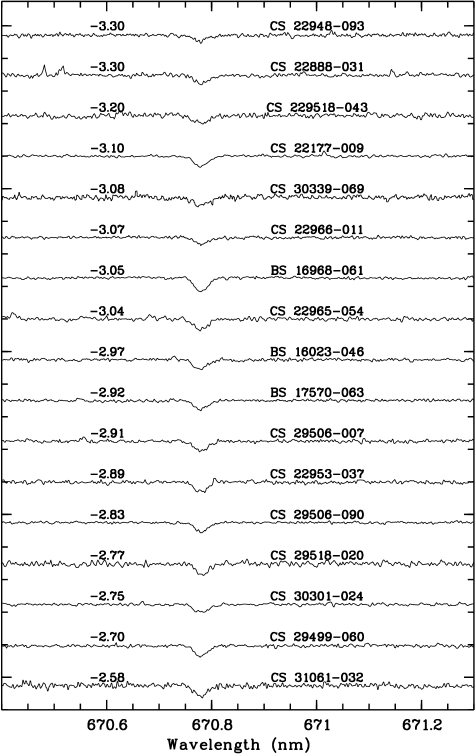
Figure 1: The Li I doublet in the 17 single main-sequence turnoff (TO) stars of our sample. Multiple spectra of each star have been coadded and normalized; for clarity, they are shifted vertically by arbitrary amounts, one tick on the vertical axis corresponding to 0.2 in residual intensity. Each spectrum is labelled with the name and [Fe/H] of the star. The stars are shown in order of increasing [Fe/H] from top to bottom.

2 Observations and data reduction

Our spectroscopic data were obtained as a part of the ESO Large Programme “First Stars”; the log of observations is given in Table First stars VII. Lithium in extremely metal poor dwarfs . We used the VLT-Kuyen 8.2m telescope and the UVES spectrograph (Dekker et al. 2000) in two non-standard settings, both with dichroic # 1: 396+573, 396+850; the numbers are the central wavelength in nm in the blue and red arms, respectively. The central wavelengths in the red arm were chosen in such a way that both settings would cover the Li doublet, essentially doubling the number of Li spectra for each star.

Most of the observations were made with a projected slit width of $1^{\prime\prime}$, yielding a resolving power of $R=43000$. Equivalent-width measurements for unblended lines were accomplished by fitting Gaussian profiles, using the genetic algorithm code described in François et al. (2003). The last column of Table 1 lists the S/N ratio per pixel near the Li line.

3 Atmospheric parameters

Our analysis used OSMARCS model atmospheres (Gustafsson et al. 1975; Plez et al. 1992; Edvardsson et al. 1993; Asplund et al. 1997; Gustafsson et al. 2003) and the turbospectrum spectral synthesis code (Alvarez & Plez 1998). Effective temperatures, $T_{\rm eff}$ , for our programme stars were determined using the wings of H$\alpha$, which is a very good temperature indicator (Cayrel 1988; Fuhrmann et al. 1993; van’t Veer-Menneret & Mégessier 1996; Barklem et al. 2002). We did not use other Balmer lines because their profiles are sensitive to the treatment of convection (Fuhrmann et al. 1993). Adopting the broadening theory of Barklem et al. (2000), we performed a $\chi^{2}$ fit of the computed profiles to the observed spectra. For the H$\alpha$ fitting we assumed log g = 4.0 for all stars.

The derived effective temperatures are about 150 K cooler than obtained previously, using the Vidal et al. (1973) theory (results presented at the IAU General Assembly in 2003; see Bonifacio et al. 2003). The error in our effective temperatures is only very weakly dependent on the photon noise, given the large number of pixels in our spectra ($\sim 5\times 10^{4}$) that define the H$\alpha$ wings. A Monte Carlo simulation showed that at S/N=50/1 the error is of only 12 K.

A more important source of error is the slight gravity dependence of H$\alpha$, which is about $-50$ K for a change of +0.25 dex in log g. In principle, it is possible to re-determine $T_{\rm eff}$ after log g has been determined from the iron ionization equilibrium (see below) and iterate the process. The worst possible case is CS 22888-031 ($T_{\rm eff}$ = 6151 K, log g = 5.00), which, after the iterations, would end up at a $T_{\rm eff}$ 150 K lower and a log g 0.25 dex lower. In practice, we feel that our gravities (based on at most four Fe ii lines) are too inaccurate to use this approach. Although internally self-consistent, this method would have introduced more scatter in $T_{\rm eff}$ than is implied by our assumption of equal gravity for all stars (for the purpose of the $T_{\rm eff}$ determination).

A further source of uncertainty is residual curvature and fringing in the echelle orders and uncertainties in the order merging. These effects are not easily modelled; to obtain a crude estimate of the associated errors, we used our observed spectra as templates and introduced the same “wiggles” on a synthetic spectrum. We then performed a model fit to this simulated spectrum and recovered effective temperatures, which could differ up to about 40 K from the effective temperature of the model used to compute the synthetic spectrum.

Another source of error is the finite pixel size in our spectra. If we rebin a synthetic spectrum (computed at a resolution $R=500,000$) to the same binning as our observed spectra and fit it again, we recover an effective temperature that may differ by up to 50 K from the input one, the average error being of about 20 K. By summing these errors linearly (we consider these errors as systematic), we estimate a total error on $T_{\rm eff}$   of about 130 K. Although this estimate has been obtained in a somewhat crude manner, we believe there is little prospect for refining it. Errors as small as 50 K are clearly not realistic, while errors as large as 200 K appear unlikely. For the rest of our discussion it would make little difference if the error is 110 K or 150 K. Note that this estimate does not include any systematic errors in the line broadening theory; as implied above, this may be in the range 150-200 K. The determination of temperatures by colours is discussed below (see Sect. 5.4).

For each star, we initially adopted a surface gravity of log g = 4.0 and used the metallicity derived in Bonifacio et al. (2003). With these parameters and the H$\alpha$-based $T_{\rm eff}$ , we interpolated a model atmosphere within a grid of OSMARCS models that was specifically computed for our application, over the metallicity range $\rm-4\leq[Fe/H]\leq-2$, with abundances of the $\alpha$ elements enhanced by 0.4 dex. Using the equivalent widths of the lines listed in Tables First stars VII. Lithium in extremely metal poor dwarfs , First stars VII. Lithium in extremely metal poor dwarfs , First stars VII. Lithium in extremely metal poor dwarfs , and First stars VII. Lithium in extremely metal poor dwarfs , where the adopted log gf values and their references are also listed, we determined the abundance of Fe i and Fe ii. The microturbulent velocity was adjusted by requiring that strong lines and weak lines yield the same abundance. The process was iterated by adjusting the gravity until an iron ionization equilibrium was achieved to within 0.05 dex. The final derived atmospheric parameters are listed in Table 1. The line-to-line scatter for Fe i was typically in the range 0.10 to 0.15 dex. As the reference solar iron abundance, we adopted A(Fe)_☉= 7.51, which is the value determined by Anstee et al. (1997) and which coincides with the meteoritic value. The [Fe/H] given in Table 1 is the mean Fe i abundance.

4 Lithium abundances

The equivalent width (EW) of the Li I doublet for each star was measured by fitting a synthetic profile, following the procedures discussed by Bonifacio et al. (2002). The EW errors listed in Table 1 were estimated using Monte Carlo simulations, in which Poisson noise was added to a synthetic spectrum to reach the same S/N ratio as the observed spectrum. However, the Poisson noise is not the only source of error in the EWs. At the wavelength of the Li doublet, CCD detectors show effects of “fringing”, which is never totally removed by flat-fielding. Residual fringing is always present at the level of a few per cent, and may introduce even larger errors than Poisson noise.

For our data, we estimated this effect by comparing results for the same star as obtained from spectra in the 573 nm setting (where the Li doublet falls on the EEV CCD) and in the 850 nm setting (where the Li doublet falls on the deep-deletion MIT CCD), which show different fringing patterns. We also compared measurements of the same star on different dates, when the Li line falls on a different portion of the fringing pattern. We conclude that residual fringing may introduce an error of about 0.1 pm, which dominates over Poisson noise. An error of 0.1 pm in the EW results in an error of 0.03 dex in the derived lithium abundance.

We used turbospectrum and the model atmosphere with parameters determined in Sect. 3 to iteratively compute synthetic spectra of the doublet until the synthetic EW matched the measured EW to better than 1%. The adopted atomic data for the Li doublet is the same as that used by Asplund et al. (2006), thus taking into account the hyperfine structure of the lines and also the isotopic components, for an assumed solar isotopic ratio. Note that changes in the isotopic ratio or even neglect of the isotopic structure have no effect on the Li abundance derived from these weak lines. The various steps of the iteration provide a curve of growth for the Li doublet, which we used to determine the error in A(Li) arising from the error in EW. For each star we also determined A(Li) from models with effective temperatures set to $\pm 130$ K with respect to the adopted temperature, which allowed us to determine the error in A(Li) due to uncertainty in effective temperature; this amounts to 0.09 dex. The errors arising from reasonable uncertainties in surface gravity and microturbulent velocity are less than 0.01 dex, and can be ignored. The total error in A(Li) is determined by summing the errors from EW and $T_{\rm eff}$ in quadrature. Due to the high quality of our data, the final error is dominated by the uncertainty in $T_{\rm eff}$ . In the present analysis we have adopted 1D model atmospheres, which ignore the effects of stellar granulation. Previous computations for the Sun (Kiselman 1997, 1998) and metal-poor stars (Cayrel & Steffen 2000; Asplund et al. 2003) suggest that these are not important for the Li doublet.

5 Analysis

Our full sample consists of 19 stars from the HK objective-prism survey of Beers and collaborators (Beers et al. 1985, 1992; Beers 1999), all of which had been classified as TO stars on the basis of medium-resolution spectra and photometry. The original sample consisted of 27 stars, but we have excluded two known spectroscopic binaries, three carbon-rich stars, one Halo Blue Straggler, and two Horizontal-Branch (HB) stars, from the present discussion. The carbon-rich stars are the topic of another paper in this series (Sivarani et al. 2006), and the binaries will be the subject of yet another paper.

We did not detect any Li features in either the Halo Blue Straggler or the two HB stars. This non-detection is consistent with our current understanding of both types of stars. In HB stars the Li, having already been diluted and partially destroyed during the star’s red giant-branch phase, is fully destroyed during the He-flash that brings the star onto the Zero Age Horizontal Branch (ZAHB). The study of Li in high-velocity A- and F-type stars by Glaspey, Pritchet, & Stetson (1994) clearly indicates that Li is strongly depleted in all Blue Straggler stars; Ryan et al. (2001; 2002) explain these depletions as the result of mass-transfer from a former companion.

In the remaining sample, BS~16076-006 turned out to be a cool subgiant; its Li abundance is A(Li)=1.13, considerably lower than in the other stars where detectable Li was expected. We interpret this as an effect of dilution, as predicted by standard models. It is interesting to note that an order of magnitude of the effect in subgiants may be estimated from the Li depletion isochrones of Deliyannis, Demarque, & Kawaler (1990). Once corrected for this depletion, as well as for expected NLTE effects, the pristine value of Li in this subgiant is A(Li) = 2.43 (see Fig. 2), which is above the range spanned by the Li abundances in the TO stars. From the paper of Ryan & Deliyannis (1998), an independent evaluation of the dilution of Li in halo subgiants may be also found; it leads to a similar result. However, note that the error on the depletion corrections for subgiants and giants are probably larger than those for dwarfs. Therefore the above value should be used with some caution.

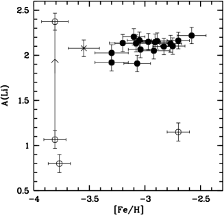
Figure 2: Derived Li abundances, corrected for standard depletion and NLTE effects, vs. [Fe/H]. The open symbols indicate the cool subgiant BS~16076-006 and the two giants/HB stars of similar $T_{\rm eff}$ , CS~22896-154 and BS~16467-062 (Cayrel et al. 2004); the observed A(Li) and the value corrected for standard depletion for BS~16076-006 are connected by an arrow; the asterisk is CS~29527-015, which is a double-lined spectroscopic binary.

From spectra taken over several runs, we find CS~29527-015 to be a double-lined spectroscopic binary (SB2). On our spectra, the measured EW of the Li doublet varies from 1.0 pm to 1.8 pm, far more than our expected observational error. This presumably reconciles the non-detection of Li in this star by Thorburn (1994) and Norris et al. (1997) with the Li detection by Spite et al. (2000); continuum light from the companion star could easily fill in the weak Li doublet (see the analysis of the SB2 CS 22876-032 by Norris et al. 2000).

Table 1: Atmospheric parameters and Li abundances

Star	V	K	$T_{\rm eff}$	log $g$	$\xi_{\rm t}$	[Fe/H]	EW	$\sigma_{EW}$	A(Li)	A(Li)c	$\mathrm{\sigma}_{A(Li)}$	S/N
	mag	mag	K	cgs	${\rm km\,s}^{-1}$	dex	pm	pm	dex	dex	dex	@670nm
BS~16023-046	14.17	12.93	6364	4.50	1.3	-2.97	1.93	0.060	2.18	2.15	0.09	186
BS~16076-006	13.44	11.69	5199	3.00	1.4	-3.81	1.29	0.080	1.07	2.37	0.09	224
BS~16968-061	13.26	11.89	6035	3.75	1.5	-3.05	2.79	0.032	2.12	2.17	0.09	289
BS~17570-063	14.51	13.19	6242	4.75	0.5	-2.92	1.76	0.040	2.05	2.05	0.09	200
CS~22177-009	14.27	13.03	6257	4.50	1.2	-3.10	2.42	0.030	2.21	2.20	0.09	178
CS~22888-031	14.90	13.58	6151	5.00	0.5	-3.30	1.87	0.040	2.01	2.03	0.09	157
CS~22948-093	15.18	14.01	6356	4.25	1.2	-3.30	1.19	0.060	1.94	1.92	0.09	181
CS~22953-037	13.64	12.43	6364	4.25	1.4	-2.89	1.95	0.030	2.16	2.16	0.09	284
CS~22965-054	15.10	13.45	6089	3.75	1.4	-3.04	2.21	0.060	2.03	2.06	0.09	150
CS~22966-011	14.55	13.28	6204	4.75	1.1	-3.07	1.37	0.050	1.90	1.91	0.09	257
CS~29499-060	13.03	11.82	6318	4.00	1.5	-2.70	2.07	0.060	2.18	2.16	0.09	163
CS~29506-007	14.18	12.92	6273	4.00	1.7	-2.91	2.05	0.040	2.15	2.15	0.09	223
CS~29506-090	14.33	13.06	6303	4.25	1.4	-2.83	1.85	0.050	2.12	2.10	0.09	222
CS~29518-020	14.00	12.70	6242	4.50	1.7	-2.77	2.10	0.110	2.14	2.13	0.09	105
CS~29518-043	14.57	13.37	6432	4.25	1.3	-3.20	1.72	0.110	2.17	2.14	0.09	107
CS~29527-015	14.25	13.02	6242	4.00	1.6	-3.55	1.86	0.060	2.07	2.08	0.09	121
CS~30301-024	12.95	11.64	6334	4.00	1.6	-2.75	1.77	0.060	2.12	2.10	0.09	183
CS~30339-069	14.75	13.47	6242	4.00	1.3	-3.08	2.04	0.110	2.13	2.13	0.09	117
CS~31061-032	13.90	12.59	6409	4.25	1.4	-2.58	2.10	0.060	2.25	2.22	0.09	116

Table 2: Parametric fits in the A(Li)–[Fe/H] plane, 17 points

	Method
$\rm A(Li)=3.20(\pm 0.37)+0.37(\pm 0.13)\times[Fe/H]$	BCES
$\rm A(Li)=2.76\pm 0.33)+0.22(\pm 0.11)\times[Fe/H]$	fitxy e $\chi^{2}=10$ ; P = 0.78
$\rm A(Li)=2.92(\pm 0.40)+0.28(\pm 0.13)\times[Fe/H]$	fitexy  $\chi^{2}=9.5$ ; P = 0.85

5.1 Dispersion in the plateau

After removing the two stars discussed above, the sample of TO stars we can use to probe the Spite plateau comprises 17 stars. The straight mean A(Li) of the sample is A(Li) $=2.11\pm 0.094$ (s.d.). The error budget is totally dominated by the error on $T_{\rm eff}$ and totals about 0.09 dex, even if we adopt an error of 0.1pm for the EW of the Li doublet, thus leaving no room for any intrinsic scatter in the plateau. Of course, this relies on our estimate of the error on $T_{\rm eff}$; if the true errors on $T_{\rm eff}$ are smaller, a small amount of intrinsic scatter in A(Li) cannot be completely ruled out.

In their analysis of the Spite plateau, Bonifacio & Molaro (1997) corrected the measured Li abundances for the effects of both standard depletion and NLTE. Similarly corrected values for our present sample are listed in Col. 9 of Table 1. Both effects are rather small, due to the high effective temperatures of our TO stars. With the corrections, the mean A(Li) lowers slightly to A(Li) = 2.10, but there is hardly any change in standard deviation (0.087 dex vs. 0.094 dex). Thus, the statistical properties of the sample change very little whether we consider the measured A(Li) or the “corrected” A(Li). The following discussion refers throughout to the “corrected” A(Li), which we simply call A(Li). It is suggestive that the dispersion is slightly reduced when the NLTE and depletion corrections are included, which suggests that those corrections are not far from the truth.

5.2 The A(Li)–[Fe/H] plane

Figure 2 shows A(Li) versus [Fe/H] for our final sample of 17 stars. At first glance, a slope of A(Li) with [Fe/H] seems to exist. However, Kendall’s $\tau$ test yields a probability of correlation between these variables of 87%; usually, correlations with a probability of less than 95% are not considered real. For example, if we remove CS~31061-032 (the most metal-rich star) from the sample and recalculate the statistic, the correlation probability drops to 66%.

Table 2 shows the results of several parametric fits to the data, including the BCES algorithm (Akritas & Bershady 1996), a least-squares fit with errors in the dependent variable only (fitxy, Press et al. 1992), and a least-squares algorithm with errors in both variables (fitexy, Press et al. 1992). The BCES and fitexy fits formally indicate a possible slope, but only at slightly more than 3$\sigma$ significance, confirming the negative result of the non-parametric test discussed above. It is interesting to note that a simulation of 10000 bootstrap samples, extracted from the real data set, fitted with BCES, provides a mean slope of 0.439, but a standard deviation of 0.387, indicating that the slope is driven by a few data points. When the most deviant points are excluded from the bootstrap sample, essentially no slope is detected. A preliminary analysis of this sample was presented at the 2003 IAU General Assembly (Bonifacio et al. 2003), where we reported the detection of a similar slope to that obtained by fitexy. The main difference in comparison to the former analysis is the removal from the sample of a few stars.

5.3 The A(Li) – $T_{\rm eff}$ plane.

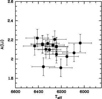
Figure 3: Derived Li abundances, corrected for standard depletion and NLTE effects, versus $T_{\rm eff}$. The asterisk denotes the double-lined spectroscopic binary CS~29527-015.

Figure 3 shows A(Li) versus $T_{\rm eff}$ for our sample. There is no clearly detectable slope in this case. Kendall’s $\tau$ provides a probability of 87% of a positive correlation. Neither of the two parametric fits detects a slope at greater than 2$\sigma$ significance.

Table 3: Parametric fits in the A(Li)–$T_{\rm eff}$ plane

	Method
$\rm A(Li)=-9.0(\pm 43)+0.18(\pm 0.69)\times(T_{eff}/100)$	BCES
$\rm A(Li)=1.07(\pm 1.32)+0.02(\pm 0.02)\times(T_{eff}/100)$	fitxye $\chi^{2}=14$ ; P $=0.53$
$\rm A(Li)=-1(\pm 3)+0.05(\pm 0.04)\times(T_{eff}/100)$	fitexy $\chi^{2}=13$ ; P = 0.62

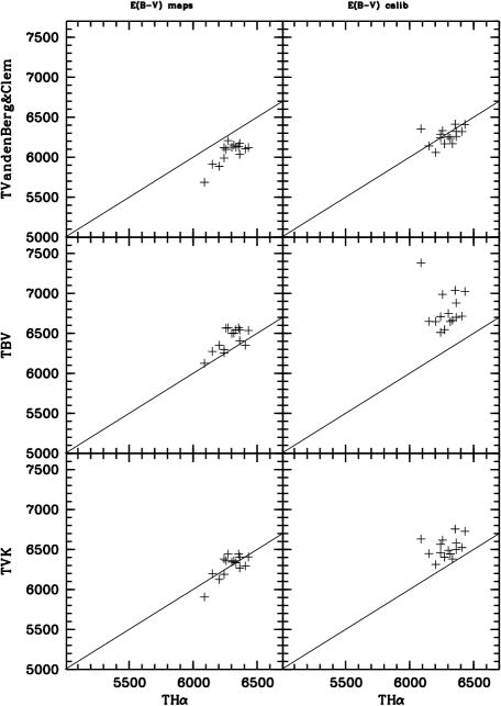
Figure 4: Comparison of different colour temperatures with the H$\alpha$ scale. From top to bottom we show the temperatures derived from $V-K$, and the Alonso, Arribas, & Martínez-Roger (1996) calibration, $B-V$ using the VandenBerg & Clem (2003) theoretical colours, and $B-V$ and the Alonso, Arribas, & Martínez-Roger (1996) calibration. The panels on the left adopt the reddening derived from the Schlegel et al. (1998) maps, corrected as in Bonifacio et al. (2000a). The panels on the right adopt the reddenings derived from the Bonifacio et al. (2000b) intrinsic colour calibration. In each panel the one-to-one relation is shown as a solid line.

Figure 5: Comparison of the different effective temperature scales based on $V-K$. The lower panels show the difference from the H$\alpha$ based temperature of the Ramírez & Meléndez (2005) calibration. The upper panels show the same for the Alonso, Arribas, & Martínez-Roger (1996) calibration. Note the different vertical scales in each panel. The panels on the left assume the reddening derived from the Schlegel et al. (1998) maps, while those on the right use the reddening that was deduced from the Bonifacio et al. (2000b) calibration.

5.4 Effects of different $T_{\rm eff}$ scales

The slope of A(Li) versus [Fe/H] described in Sect. 5.2, detected at slightly over 3$\sigma$, is of the order of 0.4 dex/dex, more than a factor of two larger than that reported by Ryan, Norris, & Beers (1999). A lively debate exists, both about the reality of this slope and, if real, about its interpretation. Bonifacio (2002) re-analysed a subsample of the stars from Ryan, Norris, & Beers (1999) for which he had accurate IRFM temperatures, but was unable to detect any slope using the published Li equivalent widths and metallicities. Recently, Meléndez & Ramírez (2004) analysed a sample of 62 metal-poor dwarfs from the literature, using IRFM effective temperatures, and again found no detectable slope. This result might be taken as confirmation of the conclusions of Bonifacio & Molaro (1997). Note that the offset in mean A(Li) of the plateau between Bonifacio & Molaro (1997) and Meléndez & Ramírez (2004) is due essentially to the different model atmospheres employed (ATLAS overshooting models by Meléndez & Ramírez 2004 vs. ATLAS non-overshooting models by Bonifacio & Molaro 1997). Thus, a slope may appear or disappear, depending on the temperature scale used. In this paper we have used H$\alpha$-based effective temperatures, which are usually found to be on the same scale as IRFM temperatures (Gratton et al. 2001; Barklem et al. 2002).

The effect of the adopted temperature scale on the existence of a slope (and the mean value of A(Li) on the plateau) requires closer inspection. For most of our stars we had $JHK$ magnitudes from 2MASS as well as $UBV$; thus, we may consider four temperature sensitive colours: $J-H$, $J-K$, $B-V$, and $V-K$. When deducing temperatures from colours one is always confronted with the problem of reddening. We decided to explore two different approaches, to be able to estimate the uncertainty on the reddening also. We used the $E(B-V)$ derived from the reddening maps of Schlegel et al. (1998), corrected as in Bonifacio et al. (2000a), as well as the $E(B-V)$ derived from the Bonifacio et al. (2000b) intrinsic colour calibration. The latter requires KP and HP indexes, which were available for all of our stars from the medium-resolution HK-survey spectra.

We note that the Bonifacio et al. (2000b) relation is derived for stars that are more metal-rich than [Fe/H] = –2.5. Thus, for all our stars we are applying an extrapolation beyond its stated range of validity. It is nevertheless interesting to compare these two $E(B-V)$ values for each star. On average, the Schlegel et al. (1998) maps yield a reddening 0.05 mag smaller than the alternative calibration (the dispersion about the mean is of similar size as the offset, $\sim$ 0.04 mag).

Bonifacio et al. (2000b) noted that an offset of 0.01 mag exists between their calibration and the reddening derived from the Schlegel et al. (1998) maps. In this case the offset appears considerably larger; however, the dispersion is compatible with the expected accuracy of each method, which is $\sim$0.02 mags for the maps and 0.03 mags for the calibration. Using these two values for the reddening, we derive effective temperatures from the Alonso, Arribas, & Martínez-Roger (1996) calibrations for all four colours. The Alonso, Arribas, & Martínez-Roger (1996) calibration for $V-K$ is given in the Johnson system; we therefore used the transformation given in Cutri et al. (2003) to transform the 2MASS $K$ magnitude to the Bessell & Brett (1988) homogenized system. The $J-H$ and $J-K$ calibrations are given for the TCS system; since a direct transformation 2MASS to TCS is not available, we performed a two-step calibration: 2MASS to CIT using the transformation of Cutri et al. (2003), and then CIT to TCS using the transformation of Alonso et al. (1994). For $B-V$ we determined $T_{\rm eff}$ using both the Alonso, Arribas, & Martínez-Roger (1996) calibration and the theoretical colours of VandenBerg & Clem (2003).

The IRFM $T_{\rm eff}$ scale has been recently revised by Ramírez & Meléndez (2005), who added a few metal-poor stars to the original sample of calibrators of Alonso, Arribas, & Martínez-Roger (1996), and computed new polynomial fits. We also considered the $V-K$ calibration of Ramírez & Meléndez (2005); in this case the calibration is performed assuming $V$ in the Johnson system and $K$ in the 2MASS system. Figure 4 shows a comparison of some of the colour-based effective temperatures with those derived from H$\alpha$. The plot suggests that offsets exist among the temperatures derived from different colours, for any chosen $E(B-V)$, as well as with respect to the $H_{\alpha}$ temperature. For some choices the colour-based $T_{\rm eff}$ and the H$\alpha$ temperature appear in good agreement; this is the case for both the $V-K$ temperature with the Schlegel et al. (1998) reddenings and the $T_{\rm eff}$ obtained from $B-V$ with the VandenBerg & Clem (2003) colours and the Bonifacio et al. (2000b) reddening corrections.

We wish to look more closely at the V-K calibrations of Alonso, Arribas, & Martínez-Roger (1996) and Ramírez & Meléndez (2005). For this purpose, from the sample of 17 stars we exclude BS 16968-061, which has no 2MASS photometry, and BS 17570-063, which lacks some of the spectral information needed by the Bonifacio et al. (2000b) calibration. With the Bonifacio et al. (2000b) reddenings, we note that both the Alonso, Arribas, & Martínez-Roger (1996) and the Ramírez & Meléndez (2005) calibrations provide higher temperatures than those estimated from H$\alpha$, Ramírez & Meléndez (2005) being by far the hottest. Furthermore, the differences are larger for the more metal-poor stars, as clearly seen in Fig. 5.

On the other hand, when the reddening based on the Schlegel et al. (1998) maps is adopted, there appears to be no trend with metallicity. In this case the mean difference $\rm T_{{(V-K)}_{A96}}-T_{H\alpha}$ is only 7.5 K with a standard deviation of 100 K, as compared to a mean difference $\rm T_{{(V-K)}_{RM05}}-T_{H\alpha}$ of 265 K, with a standard deviation of 122 K. None of the above discussed residuals shows any trend with $T_{\rm eff}$ . We conclude that the IRFM-based temperatures derived from the Alonso, Arribas, & Martínez-Roger (1996) calibration are in good agreement with the H$\alpha$ temperatures, even for these extremely low metallicities, in keeping with what is found at higher metallicities (Gratton et al. 2001; Barklem et al. 2002). On the other hand, the temperatures derived from the Ramírez & Meléndez (2005) calibration are considerably higher and essentially incompatible with the H$\alpha$ temperatures. These discrepancies suggest that a systematic error in the adopted temperature scale of the order of 200 K is still possible.

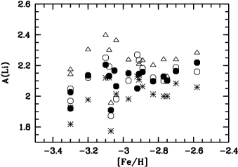
Figure 6: Effect of different temperature scales on the Spite plateau. Filled circles: H$\alpha$ scale; open circles: $V-K$ with reddening from the Schlegel et al. (1998) maps; open triangles: $V-K$ with reddening from the Bonifacio et al. (2000b) calibration; asterisks: $B-V$ from VandenBerg & Clem (2003) and reddening from the Schlegel et al. (1998) maps.

To illustrate the effects of different temperature scales on the Spite plateau, Fig. 6 compares A(Li) as derived with the H$\alpha$ temperatures with that derived using three other $T_{\rm eff}$ scales. The comparison is slightly inconsistent, since we did not recompute [Fe/H] with the different $T_{\rm eff}$ scales, only A(Li). However, we believe this is sufficient to illustrate the general trends. Figure 6 shows that, although the $V-K$ temperatures (with the Schlegel et al. (1998) reddening) and the H$\alpha$ temperature (which should not be affected by reddening) appear to be on the same scale, the Spite plateau has a very different appearance in the two cases. With the H$\alpha$-based temperatures there is (weak) evidence for a slope in A(Li) vs. [Fe/H]; when using the $V-K$ temperatures there is no evidence for a slope (but the scatter in A(Li) is larger in this case). The most extreme situation is when we adopt the Ramírez & Meléndez (2005) $V-K$ calibration and the reddenings from the Bonifacio et al. (2000b) calibration – not only is there no slope (probability of correlation of 2%), but two stars have A(Li) $\sim 2.6$, and one star would be assigned essentially a meteoritic Li abundance. This is a consequence of the fact that in this case the temperature difference with respect to the H$\alpha$ scale is larger at lower metallicities. This trend may be totally spurious, and arise from the fact that we are extrapolating the Bonifacio et al. (2000b) calibration beyond its range of validity.

We note here that our H$\alpha$ temperatures yield an excitation equilibrium for iron, i.e., no detectable abundance trend with excitation potential, for most of our stars (13 out of 19). For those in which a mild slope was found (at most 0.06 dex/eV), it could be removed by adopting a slightly cooler $T_{\rm eff}$, by 100 K in the worst cases. In contrast, with the high $T_{\rm eff}$ derived from the Ramírez & Meléndez (2005) calibration, no iron-excitation equilibrium is achieved; remaining slopes are of the order of 0.15 dex/eV. Furthermore, achieving iron-ionization equilibrium in such cases would require substantially larger surface gravities, as large as log g = 5.5 in some cases, which is very unlikely in TO stars. We conclude that the Alonso, Arribas, & Martínez-Roger (1996) calibration is in good agreement with both H$\alpha$ temperatures and iron excitation temperatures.

5.5 Comparison with the results of Asplund et al.

In a recent paper Asplund et al. (2006, , hereafter A06) measured both ⁶Li and ⁷Li from UVES spectra for a sample of 24 metal-poor stars. To investigate ⁶Li, which has a very small isotopic separation from ⁷Li, the S/N ratios of their spectra had to be extremely high, and therefore their measured equivalent widths are of very high accuracy as well. Their adopted temperature scale is based on the wings of H$\alpha$, modelled with the Barklem et al. (2000) broadening theory, and is thus, in principle, identical to ours.

Since we have no stars in common with A06, and at the suggestion of the referee, we downloaded UVES spectra from the ESO archive for two of the most metal-poor stars in the sample of A06, LP 815-43 and CD –33 1173. These data include the spectra used by A06, taken with the image slicer, as well as other spectra taken with a slit, which are more similar to our own data. The details of the analysis of H$\alpha$ from these data is shown in the appendix, and the spectra used are detailed in Table A. The main result is that, even taking into account the different data available and the differences in data reduction and line-profile fitting, our temperature scale agrees with that of A06, although a zero point shift of up to to 40 K is possible. To be certain on this point, we should determine effective temperatures for a large fraction, if not all of, the stars in the A06 sample. This is clearly beyond the scope of the present paper.

We also used these data to compare the metallicity scales. Table A lists our measurements of iron lines for LP 815-43. These data, analysed with the $T_{\rm eff}$ = 6400 K used by A06 and our models and atomic data, provides [Fe/H]=–2.94, log g = 3.90, and $\xi=1.6$  ${\rm km\,s}^{-1}$ . We conclude that the metallicity scales of the present paper (based on neutral iron lines) and that of A06 (based on ionized iron lines) are offset by $\sim 0.2$dex, in the sense that our analysis provides lower metallicities. A06 find a mean difference between A(Fe i) and A(Fe ii) of 0.08 dex, which suggests that the offset between the metallicity scales is not entirely due to the use of neutral or ionized iron, but may also be related to differences in the choice of lines, the adopted atomic data, and, possibly, also the line formation codes. It is interesting to note, however, that the study of metal-poor subgiants by García Pérez et al. (2006), who adopt the same approach and methods as A06, finds a mean imbalance of 0.19 dex between neutral and ionized iron, virtually identical to the offset we are discussing. It may well be that, after all, the line-to-line scatter for both Fe i and Fe ii is too large to allow strong conclusions on the ionization balance, and, consequently, on surface gravities. Whatever the case, for the purpose of the present comparison we applied this shift to the A06. Although a thorough re-analysis of their spectra would be preferable, again, it would be beyond the purpose of the present paper.

We finally compared the derived A(Li) abundances. Somewhat to our surprise, we found that using the equivalent widths published by A06, and their adopted atmospheric parameters, with the use of turbospectrum the derived lithium abundance is about 0.04 dex higher than the one found by the A06 study. In spite of extensive investigations, with the collaboration of M. Asplund, we were unable to resolve the reason of this discrepancy. We did, however, ascertain that this small offset is not due to the models employed, to the adopted atomic line data, or to the adopted continuum opacities. This finding indicates the likely level of systematic error in derived Li abundances due to the use of different spectrum synthesis codes. For the present comparison we recomputed all of the Li abundances using the equivalent widths and model parameters of the A06 study. The A06 “rescaled” data is plotted in Fig.7, together with our own. The fact that now the most metal–poor stars of the A06 sample fall in the midst of our measurements supports the notion that the adopted rescaling in [Fe/H] and the re-computation of A(Li) have brought the two samples onto the same scales.

Figure 7: Comparison of our sample (filled circles), with that of A06 (open circles). The temperature scale of both samples is based on H$\alpha$ profiles.

As was pointed out by Cayrel et al. (2004), Mg is perhaps a better reference element to study chemical evolution, since its production in relatively external layers of massive stars is linked to the volume of the Li-poor external layers more directly than to the volume of the deep iron-rich ejected layers, which depend on additional parameters (fallback and mass cut). In Fig. 8 we plot A(Li) as a function of [Mg/H]. Magnesium has typically been measured using 7 lines for each star, and should be quite accurate; details will be given in a forthcoming paper of this series (Spite et al., in preparation, see also Spite et al. 2005). For the A06 data, we estimate Mg abundances from their [O/H] measurements by adopting [Mg/H] = [O/H]–0.46, since we find a mean [Mg/O]= –0.46 for our giants (Cayrel et al. 2004), and [Mg/O] is constant with [Mg/H] (see Fig. 13 of Cayrel et al. 2004).

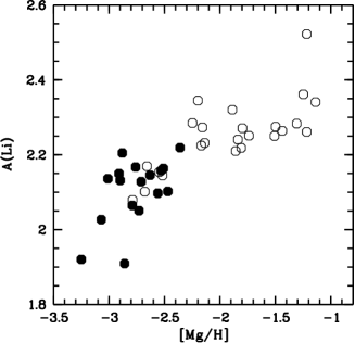
Figure 8: Comparison of our sample (filled circles), with that of A06 (open circles) using Mg as a reference element. For the stars of A06 Mg has been estimated by rescaling their oxygen measurements (see text).

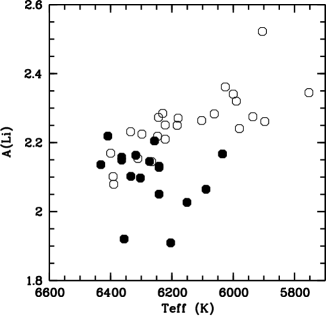
Figure 9: Comparison of our sample (filled circles), with that of A06 (open circles) in the Li-$T_{\rm eff}$ plane.

Figure 9 displays A(Li) versus $T_{\rm eff}$ for the two samples. It is clear that, while our data do not exhibit any slope with $T_{\rm eff}$, the data of A06 exhibit a sizeable slope of about $-0.04$ dex/100 K, the hotter stars exhibit the lowest Li abundances. This may be related to the structure of the A06 stellar sample, which shows a strong correlation between [Fe/H] and $T_{\rm eff}$, their most metal-poor stars are also the hottest. We stress that the A(Li) vs. $T_{\rm eff}$ slope is in the opposite direction of that found by Ryan et al. (1996). Note as well that for the most metal-poor stars of the sample described by Charbonnel & Primas (2005), there exists a slope similar to that of Asplund et al., although it is not very well defined. Also, Ryan et al. (2001) provide a figure of A(Li) versus $T_{\rm eff}$, which suggests a changing slope for the hottest stars, but only as a subtle effect.

6 Discussion

The two main reasons that drove our investigation were, first, to understand whether the interpretation of a primordial origin of the Spite plateau is supported by the new observations of the most metal–poor stars, and secondly, if this is the case, to assess the value of the primordial Li abundance. In this context, the existence or non-existence of a slope in A(Li) versus [Fe/H] in the Spite plateau plays an important role. It is possible that a real slope may indicate either that there has been Li production by cosmic rays in the early Galaxy, as suggested by Ryan et al. (2000), or that some atmospheric phenomenon, such as diffusion, has altered the atmospheric Li abundance in a metallicity-dependent manner, or even that a metallicity-dependent astration of Li in the progenitors, as proposed recently by Piau et al. (2006), may exist. In the first case the primordial Li abundance might be estimated by simply extrapolating the slope down to very low metallicities, while in the other cases the primordial abundance cannot be estimated in a model-independent way.

6.1 The scatter in the plateau

As has been found by all (recent) investigations, based on data of the highest quality, we confirm a very low scatter in the Li abundances among stars on the Li plateau, a scatter which may be explained by observational errors alone. However if we arbitrarily divide the sample of 17 stars into two subsamples, one with [Fe/H]$\leq-3.0$ (8 stars) and its complement (9 stars), we find a scatter of 0.11 dex for the lower-metallicity subsample and 0.05 dex for the higher-metallicity subsample. The increased scatter in A(Li) for the lowest metallicities could be due to the fact that they are TO stars. The transition between the dwarf and subgiant phase may produce some transport processes that result in a reduction of photospheric Li in these stars, but this remains to be confirmed by further study, and empirical data suggest the contrary (Charbonnel & Primas 2005).

6.2 The slope of the plateau

From our measurements alone the evidence for any slope in A(Li) vs. [Fe/H] in the Spite plateau is weak. Its existence or non-existence remains a very delicate issue, the resolution of which will likely require temperatures with accuracies of the order of 50 K, roughly a factor of two better than what can be achieved at present. The larger scatter in A(Li) when the $V-K$ temperatures are adopted can be ascribed to a larger error on estimated $T_{\rm eff}$, as compared to that obtained using the H$\alpha$-based temperatures. We attribute this error to being dominated by the uncertainty in the reddening, which will always prevent one from obtaining accurate temperatures from colours alone.

The situation is totally different when we look at the combined sample formed from our stars and those of A06. In this case, sizeable slopes exist, both with $T_{\rm eff}$ and with [Fe/H], which are, however, entirely driven by the A06 data at higher metallicity. We note that while A06. stress the existence of a slope with [Fe/H] in their data, they do not comment or even mention the existence of a steep slope with $T_{\rm eff}$.

We are thus faced with surprising and somewhat contradictory information. The correlation between [Fe/H] and A(Li) is clearly present, with a slope of about 0.15 dex/dex. The impression one obtains from inspection of Fig. 7 is that of an almost vertical drop of lithium abundance at the lowest metallicities. The fact that the A06 data also displays a steep slope with $T_{\rm eff}$, in the opposite direction of that which has been found by previous investigations, suggests that A06 may have unveiled a new physical phenomenon for the first time (see Sects. 6.5 and 6.7 for possible interpretations). This is, of course, predicated on the absence of a systematic temperature-dependent error in the adopted $T_{\rm eff}$ scale.

Note that for LP 815-43, which is one of the stars that outline the slope, Meléndez et al. (2006) derive $T_{\rm eff}$ = 6622 K, 222 K higher than the $H\alpha$-based $T_{\rm eff}$. If one were to adopt this $T_{\rm eff}$, the derived A(Li) would rise to 2.3, i.e., at the level of the less metal–poor stars. It is clear from figure 8 of Meléndez et al. (2006), and confirmed by our own analysis, that their temperatures are considerably hotter than H$\alpha$-based temperatures only for the extremely metal-poor stars. Our analysis disfavours the Ramírez & Meléndez (2005) temperature scale, on account of its inconsistency with the iron excitation equilibrium. However, it is unclear at this stage whether the increase in the difference between the Ramírez & Meléndez (2005) $T_{\rm eff}$ estimates and H$\alpha$-based $T_{\rm eff}$ estimates with decreasing metallicity reflects a problem in the H$\alpha$ scale, in the Ramírez & Meléndez (2005) scale, or both.

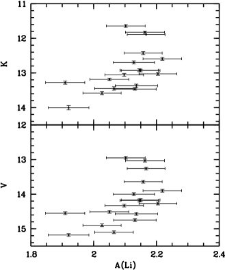
Figure 10: Li abundance vs. apparent $V$ and $K$ magnitudes. Kendall’s $\tau$ test indicates a correlation at over the 99% level in both cases.

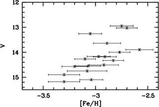
Figure 11: [Fe/H] vs. apparent $V$ magnitude. Kendall’s $\tau$ test indicates a correlation at over the 99% level.

We find it somewhat disturbing that, at least in our present sample of stars, a slope of A(Li) with apparent magnitude exists, as shown in Fig. 10. The slope is obvious, whether one employs $V$ or $K$ magnitudes; the fainter stars have lower derived Li abundances. The correlation is detected at over the 99% confidence level for both bands, and hence cannot be questioned. A correlation, with a similar confidence level, exists between apparent magnitude and [Fe/H] (Fig. 11). It is worth mentioning that this correlation between apparent magnitude and A(Li) is not peculiar to our sample. The 62 stars in Charbonnel & Primas (2005) with $T_{\rm eff}$ $>5700$ K and [Fe/H] $\leq-1.5$ exhibit a similar trend.

The correlation between [Fe/H] and apparent magnitude might be understood as an observational bias, such as that suggested by Bonifacio (2002). To observe a similar number of stars at [Fe/H] = –3.2 as at [Fe/H] = –2.8, one must sample a larger volume of the Galactic halo. As a result, on average, the most metal-poor stars are more distant, and their apparent magnitudes are fainter. One can easily see that if such a correlation exists along with a correlation between A(Li) and [Fe/H], then a correlation between A(Li) and apparent magnitude must exist. Moreover, the slopes in the different planes must be simply related, e.g., the slope in the [Fe/H], A(Li) plane must be the product of the slopes in the $K$, A(Li) and $K$, [Fe/H] planes, which is in fact verified.

Bonifacio (2002) also suggested that the trend of A(Li) vs. [Fe/H] may be due to observational bias. In a large sample of stars from the literature, he found a clear trend of the equivalent width of the Li doublet with metallicity. This arises because the most metal-poor stars are also the hottest. The combination of small equivalent widths and faint magnitudes may yield less accurate measurement and systematic underestimates of the equivalent widths.

In Bonifacio (2002), the slope of A(Li) vs. [Fe/H] was seen in the full sample of 73 stars, but not in the subsample of 22 stars with reported errors in equivalent widths less than 0.1 pm. The present sample has been designed to avoid such a bias, both because all of the stars are rather hot and because we obtained very high S/N ratio for all stars, independent of their apparent magnitude. Our sample does not exhibit any trend of the Li doublet equivalent width with metallicity. In our sample, 15 of 17 stars have errors on the equivalent width of the Li doublet less than 0.1 pm; the two remaining stars have errors of 0.11 pm, which shows that our goal of obtaining a uniformly high S/N ratio for all our program stars has been achieved.

The situation is therefore the following. Having established that there exists a plausible reason for the existence of a correlation between [Fe/H] and apparent magnitude (the observational bias), at least one of the two correlations A(Li) vs. apparent magnitude and A(Li) vs. [Fe/H] must have a physical origin. The other may simply be a consequence of the former two.

6.3 Li production by Galactic cosmic rays

If the trend with [Fe/H] is real, we must try to understand the physical reason for it. Ryan et al. (2000) interpreted the correlation found by them as evidence for Galactic production of Li. However, adopting this interpretation results in a primordial Li abundance in stark contradiction to SBBN (with $\eta$ derived from the WMAP observations). Extrapolating the trend of A(Li) linearly down to a metallicity of [Fe/H] = –4.0, we find A(Li) =1.80, i.e., (Li/H) $=6.3\times 10^{-11}$, compared to the minimum (Li/H) $\sim 1.13\times 10^{-10}$ predicted by our Kawano-code primordial nucleosynthesis computations. To avoid finding a primordial Li below the minimum allowed by the theoretical computations, Ryan et al. (2000) increased all their A(Li) values by 0.08 dex, arguing that this brought the zero point of their temperature scale in agreement with the IRFM temperatures.

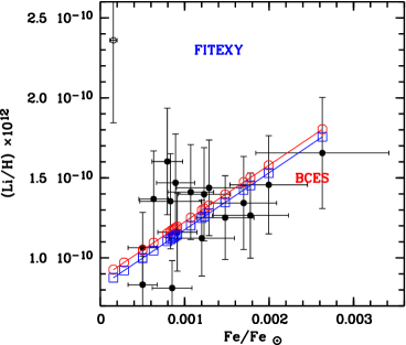
Figure 12: Fits of (Li/H) as a function of $\rm(Fe/Fe_{\odot})$.

Ryan et al. (2000) argued that an early flux of Galactic cosmic rays (GCR) should result in a lithium production that exhibits a linear trend of (Li/H) with $\mathrm{(Fe/Fe_{\odot})}$. In this case a fitting function of the form $\mathrm{(Li/H)=a+b(Fe/Fe_{\odot})}$ is more appropriate than a linear fit of the logarithmic abundances, as was discussed above. Figure 12 shows the result of such a fit. The BCES fit and fitexy provide similar results. BCES suggests $\mathrm{a}=(8.72\pm 1.71)\times 10^{-11}$ and $\mathrm{b}=(3.54\pm 1.10)\times 10^{-8}$. Extrapolation down to a metallicity of [Fe/H] = –4.0 implies (Li/H) $=8.72\times 10^{-11}$, which is higher than the logarithmic fit, but still below the minimum predicted by SBBN ((Li/H) = $1.13\times 10^{-10}$). It is clear that for all metallicities below [Fe/H] $=-4.0$, the term $\mathrm{b(Fe/Fe_{\odot})}$ is negligible compared to $\mathrm{a}$, and if we take the $\mathrm{a}$ value at $+3\sigma$ we have (Li/H)$\sim 1.61\times 10^{-10}$. We cannot avoid the conclusion that if the trend of A(Li) with [Fe/H] is due to GCR Li production, then either SBBN is wrong and should be replaced by some other theory of Li formation, or the baryonic density determined by WMAP is overestimated and should be reduced to a lower value, compatible with both the D/H and the Li/H values.

6.4 Diffusion at work?

One alternative explanation would be that the correlations between A(Li) and [Fe/H] could be caused by some metallicity- and/or temperature-dependent Li depletion mechanism. In this regard, it is of significance that recent investigations of the effects of diffusion (with the inclusion of turbulence: Richard et al. 2002; Richard, Michaud, & Richer 2002; Michaud, Richard, & Richer 2004; Richard et al. 2005) have been able to reproduce the Li-$T_{\rm eff}$ dependence found by Ryan, Norris, & Beers (1999). Richard et al. (2005), in their figure 3, show that their best-fitting model provides a curve with a mean slope vs. $T_{\rm eff}$ of 0.013 dex/100K. It is interesting to recall here, that, while our sample alone shows no trend with $T_{\rm eff}$ , when including the sample of A06 we find a slope that is considerably larger, but of the opposite sign. Could it be that we are seeing the downturn of the Spite plateau at the highest temperatures, predicted by the old diffusive models (e.g., Vauclair & Charbonnel 1995)? Here the downturn could be linked to metallicity rather than to temperature.

No curve is provided by Richard et al. (2005) to illustrate the “constancy” of A(Li) versus [Fe/H], but the text of the paper emphasises the basic facts that should lead to this constancy. The primary theme of Richard et al. (2005) is not the numerical values of the (small) slopes of A(Li) vs. $T_{\rm eff}$ and [Fe/H], but the global constancy of the modelled A(Li) on the plateau and the net depletion. These authors claim to be able, by this approach, to satisfactorily close the gap between the mean observed value of A(Li) of the plateau and the A(Li) value derived from the WMAP measurements.

Recently, Korn et al. (2006) have claimed the detection of a diffusion “signature” in the Globular Cluster NGC 6397. According to their analysis the TO stars in this cluster exhibit lower iron and lithium abundances than the slightly more evolved stars. Both these facts may be interpreted in the framework of the diffusive models of Richard et al. (2005). This result is very suggestive; however, it relies heavily on the adopted temperature scale, which is plausible, albeit inconsistent with the cluster photometry. An increase by only 100 K of the effective temperature assigned to the TO stars would remove the abundance differences between TO and subgiant stars. Previous analyses of the same cluster (Castilho et al. 2000; Gratton et al. 2001), with different assumptions on the effective temperature scale, failed to find any difference in [Fe/H] between TO, subgiant, and giant stars. Thus, we are again faced with the need to be able to determine effective temperatures to better than 50 K to confirm or refute this result.

6.5 A Population II Li dip?

Another possibility is that we are observing a phenomenon that is similar to the “Li dip” (Boesgaard & Tripicco 1986), a depletion of lithium observed within a small temperature range in some field Pop I stars and also in old open clusters. We recall that the Li dip is not observed in young clusters, but is seen in old, preferably slightly metal-poor clusters. Interpretations by diffusion (Michaud 1986; Proffitt et al. 1990), rotationally induced mixing (Böhm-Vitense 2004; Talon & Charbonnel 2003; Pinsonneault et al. 1992), or mass loss (Schramm et al. 1990) have been proposed.

The observation of a low Li content in subgiants lead Balachandran (1990) to conclude that the Li dip is due to the previous destruction of Li in the main sequence phase, which is improbable for very low-metallicity dwarfs. Balachandran (1990) found that a lithium depletion is noted in subgiants which had a temperature larger than 7000 K on the main sequence, and suggested that this depletion corresponds to the dip. At solar metallicity the dip is around the mass 1.35 $M_{\sun}$, at intermediate metallicity it is around 1.25 $M_{\sun}$, and at low metallicity it is around 1.1 $M_{\sun}$. A dip at 0.8 $M_{\sun}$ for extremely low metallicity would be in line with this trend.

Dearborn et al. (1992) have claimed that the mass-loss scenario (Schramm et al. 1990) that is capable of explaining the Hyades Li dip necessarily predicts an Li dip for Pop II stars also. In their computation, the red edge of the dip should appear at around $T_{\rm eff}$ = 6600 K, i.e., only slightly hotter than our most metal-poor stars. No Li dip has been clearly observed in Pop II stars yet; however, Fig. 9 is reminiscent of what one should see approaching the Li dip from the cool side. So, perhaps, the temperature trend discovered by A06 constitutes the first evidence in favour of a Pop II Li dip. It is unclear why previous investigations have failed to detect it, as it is unclear why it is not detected among Pop I field stars (Lambert & Reddy 2004). Such a process would not necessarily explain the low Li in the hyper iron-poor dwarf HE 1327-2326 (Frebel et al. 2005), which does not have a very low global metallicity $Z$ (Collet et al. 2006), but has a still lower mass.

6.6 The ⁶Li plateau

The measurements of ⁶Li in halo stars also have implications for the interpretation of the Spite plateau. In the 1990s a firm detection of ⁶Li was achieved for only one halo star, HD 84937 (Smith, Lambert, & Nissen 1993; Hobbs & Thorburn 1994; Smith et al. 1998; Cayrel et al. 1999). The measured ⁶Li/⁷Li ratio was of the order of 5%. Detections of ⁶Li have been claimed for only three other halo stars, but these have been withdrawn on the basis of higher quality spectra. Smith et al. (1998) claimed a detection of ⁶Li in BD $+26^{\circ}3578$ (= HD 338529) at the level of 5%, which has been changed to an upper limit by A06. The detection of ⁶Li in HD 140283 by Deliyannis & Ryan (2000) was changed to an upper limit by Aoki et al. (2004). Finally, the detection of ⁶Li in G 271-162 by Nissen et al. (2000) was changed to an upper limit by A06.

Recently, A06 claimed detection of ⁶Li in nine more halo stars. Surprisingly, these stars seem to have the same Li isotopic ratio of $\sim$ 5%, defining a ⁶Li plateau which appears to mirror the ⁷Li plateau.

Given the extreme difficulty of measuring the ⁶Li ratio and the history of several claimed detections and withdrawals, caution is advised in accepting the measurements of A06 until they are confirmed by an independent analysis, preferably based on data from a different spectrograph. However, the fact that the ⁶Li measurement in HD 84937 has been confirmed in four independent analyses suggests that it is unlikely that all the detections claimed by A06 will later be found to be upper limits. Hence, for the sake of the discussion, we shall take these measurements at face value.

The measurements of ${}^{6}\mathrm{Li}$ in halo stars imply the production of both Li isotopes by GCR at [Fe/H]$\sim-2.3$. At low metallicities, the $\alpha-\alpha$ fusion process may be competitive with spallation. The fusion process is favoured in the special environments near supernovae; thus, unless the early Galaxy was very well mixed, there should be some scatter in Li, and some stars having higher Li because they were formed from an ISM enriched by $\alpha-\alpha$ fusion. This could explain a tiny scatter; moreover, since on average it is more likely to observe such a process at higher metallicities, it may cause a slight rise of A(Li) with metallicity. This expectation is contradicted, however, by the apparent constancy of ⁶Li in halo stars.

Clearly, the 5% ${}^{6}\mathrm{Li}$ observed in HD~84937 and other halo stars is not enough by itself to produce the slope with metallicity in the Spite plateau found by Ryan, Norris, & Beers (1999) and A06. To achieve this, the ${}^{6}\mathrm{Li}$/${}^{7}\mathrm{Li}$ ratio must be higher at lower metallicities, which is again contradicted by the observations. To reconcile the absence of slope in the ⁶Li plateau with the slope in the ⁷Li plateau, Asplund et al. (2006) invoke a metallicity-dependent pre-main-sequence (PMS) depletion of ⁶Li; after correction for this, their ⁶Li data show a slope similar to that of ⁷Li. Although viable, this explanation appears somewhat contrived, and the prediction of Li destruction is less certain on the PMS than on the main sequence (Proffitt & Michaud 1989). For example, the models of Piau (2005) are marginally consistent with the ⁶Li measurements, but they do not lead to a slope in ⁶Li.

6.7 Pre-Galactic Li processing

Piau et al. (2006) suggested that the first massive supernovae have ejected large quantities of Li-poor (and D-poor) hydrogen. If these ejections are triggering local star formation, the stars so formed will have inhomogeneous Li abundances. The following yields of (more numerous) lower mass (less astration) supernovae will provide slightly higher (and more homogeneous) Li abundances. The observed Li abundance would be a reduced Li primordial abundance, especially for the most metal-poor stars of the sample, only slightly reduced for the less metal-poor ones. This scenario would not completely explain the gap between the Spite plateau and the prediction derived from WMAP, but could account for 0.2–0.3 dex. Piau et al. (2006) account for the remaining discrepancy by appealing to depletion during the lifetimes of the low-mass stars.

A massive astration of Li in half of the Pop II material has been suggested by Piau et al. (2006). This process destroys Li by a factor 2 in 2% of the mass of the Milky Way, i. e., the halo. Later the remaining 98% of the mass of the Milky Way joins the halo by infall. This infalling matter is made of primordial gas and the mixture produces the Pop I. Is this large amount of primordial gas also astrated depleting Li? Not more than by a factor of 2, if the models of chemical evolution of D in the Galaxy are to be trusted. We note in passing that all the scenarios advocating the destruction of ⁷Li imply an even larger destruction of ⁶Li. On the other hand, production of ⁶Li implies production of ⁷Li, thus some of the above scenarios may be difficult to reconcile with the ⁶Li observations.

Finally, there is the possibility of a pre-Galactic origin for both isotopes as suggested by Asplund et al. (2006). Possible ⁶Li production channels include proto-galactic shocks (Suzuki & Inoue 2002; Fields & Prodanović 2005) and late-decaying or annihilating supersymmetric particles during the era of big bang nucleosynthesis (Jedamzik et al. 2006), as mentioned below. The presence of ⁶Li limits the possible degree of stellar ⁷Li depletion and thus sharpens the discrepancy with standard big bang nucleosynthesis.

6.8 New physics

The dominant uncertainty in SBBN Li production is the cross section of the $\rm{}^{3}He(\alpha,\gamma)^{7}Be$ reaction. This has been examined in detail by Cyburt et al. (2004), who concluded that large errors in the cross section of this reaction are unlikely. The possibility that $\rm{}^{7}Be$ is destroyed by the reactions $\rm{}^{7}Be$ $(d,p)$ $\rm 2^{4}He$ and ⁷Be$(d,\alpha)^{5}$Li has been considered by Coc et al. (2004), who concluded that the issue remains open, pending accurately measured cross sections for these often-neglected reactions. However Angulo et al. (2005) have recently measured this cross section at energies appropriate to the big bang environment and find it to be a factor of 10 smaller than what was previously assumed. Thus, this possibility for reconciling the Spite plateau with the baryonic density derived from the WMAP measurement no longer appears viable. On the contrary, (Leonard et al. 2006) have recently provided a high precision measurement of the $\rm{}^{2}H({\mathit{d},\mathit{p}})^{3}H$ and $\rm{}^{2}H({\mathit{d},\mathit{n}})^{3}He$ total cross sections, which imply an increase of 0.02 dex of the predicted Li abundance, thus making the discrepancy even larger.

Other possibilities exist, e.g., using non-standard BBN to predict the abundances of the light elements. The most appealing such model is the case of a late-decaying massive particle (Jedamzik 2004a, b). However, in the case of an electromagnetic decay, this hypothesis implies either a D abundance that is too low with respect to current observations, or a $\rm{}^{3}He/D$ ratio that is too high (Ellis et al. 2005). Recently Jedamzik et al. (2006) have shown that if the late decaying particle is a gravitino, then the Spite plateau and the baryonic density determined by WMAP may be reconciled. Even more interestingly, a primordial production of ⁶Li at the level of what was observed in metal-poor stars (Smith, Lambert, & Nissen 1993; Hobbs & Thorburn 1994; Cayrel et al. 1999; A06) can also be attained for appropriate choices of the gravitino properties.

6.9 What else?

We find that none of the above scenarios is very satisfactory to describe existing data as depicted by Fig.7. However, the number of stars on which these conclusions rest is still very small, and observations of more extremely metal-poor stars are still needed to clarify the situation.

7 Conclusions

Our investigation has considerably increased the number of TO stars below [Fe/H] = –3.0 with available ⁷Li abundance estimates. The interpretation of the results is by no means straightforward. Our measurements alone do not support the existence of any slope with metallicity or $T_{\rm eff}$; however, an increase in the dispersion at the lowest metallicities or an abrupt downturn of Li abundances below [Fe/H] = –3.0 could be consistent with the data. When considering the A06 data, which after suitable rescaling should be on the same metallicity and temperature scale as our own data, sizeable slopes with [Fe/H] and $T_{\rm eff}$ are found. Our data are not in contradiction with the A06 data, being somewhat complementary, in the sense that our data populate the lowest metallicity regions. When considering the complete data set (A06 plus our own) the situation described by Fig. 7 is that of a slope with [Fe/H] and an increased scatter at the lowest metallicities. We stress again that the slope is implied only by the data of A06, relative to a sample showing a strong correlation between [Fe/H] and $T_{\rm eff}$ .

The existence of a gap between A(Li) in metal–poor stars and the primordial Li predicted by the SBBN and the baryonic density determined by WMAP is confirmed. The gap could be filled if metal–poor TO stars had effective temperatures $\sim 7300$ K, which appears inconsistent with the colours of the stars, the profiles of their H$\alpha$ lines, and their iron-excitation equilibria. The temperature scale of metal-poor stars still has a zero point uncertainty at the level of $\sim 200$ K. The iron-excitation equilibria in our stars do not support extremely high temperature scales, such as that of Ramírez & Meléndez (2005); however, our analysis does assume LTE and makes use of 1D model atmospheres. Departures from LTE and granulation effects should be investigated to assess the significance of our result. In any case, the present observations constitute a strong constraint for any theory seeking to explain the Li-WMAP discrepancy in terms of Li depletion in metal-poor stars. Parallaxes for these stars would be extremely valuable, since their TO status rests entirely on spectroscopic surface gravities, which could be affected by systematic errors in the analysis (NLTE effects on Fe i, 3D effects, etc.); these should become available around 2020 from the GAIA mission and/or SIM. The issue of the temperature scale of metal-poor stars is still not settled; a direct measurement of the angular diameter of even one metal-poor star would be extremely valuable.

[x]llllllllllllll Equivalent widths and abundances of iron lines

BS 16076-006 CS 29527-015 CS 22888-031 CS 22948-093 CS 29518-043
$\lambda$ $\chi$ log gf Ref. EW A(Fe) EW A(Fe) EW A(Fe) EW A(Fe) EW A(Fe)
nm eV pm dex pm dex pm dex pm dex pm dex

continued.

BS 16076-006 CS 29527-015 CS 22888-031 CS 22948-093 CS 29518-043
$\lambda$ $\chi$ log gf Ref. EW A(Fe) EW A(Fe) EW A(Fe) EW A(Fe) EW A(Fe)
nm eV pm dex pm dex pm dex pm dex pm dex

Fe i
337.0783 2.69 $-0.266$ BWL – – – – – – – – – –
339.9333 2.20 $-0.622$ BWL 1.54 3.57 – – 1.38 4.38 – – – –
340.1519 0.92 $-2.059$ BWL 1.37 3.54 – – – – – – – –
340.7460 2.18 $-0.020$ BWL 3.68 3.52 1.76 3.96 2.38 4.08 – – 1.54 4.06
341.3132 2.20 $-0.404$ BWL 2.03 3.51 – – —- – – – –
341.7841 2.22 $-0.676$ BWL – ———- – – – –
341.8507 2.22 $-0.761$ BWL 1.12 3.57 ——– – – – –
342.4284 2.18 $-0.703$ BWL – – – – – – – – – –
342.5010 3.05 $-0.500$ BWL – ———- – – – –
342.6383 0.99 $-1.909$ BWL – —— 0.75 4.23 – – 1.82 4.23
342.7119 2.18 $-0.098$ BWL 3.48 3.54 —- 2.53 4.20 – – – –
342.8193 2.20 $-0.822$ BWL 0.82 3.44 —- 1.17 4.49 – – – –
344.0606 0.00 $-0.673$ BWL 10.11 3.60 7.22 4.08 8.11 4.19 – – 7.25 4.52
344.0989 0.05 $-0.958$ BWL 8.83 3.64 6.00 4.03 7.35 4.39 – – 6.25 4.51
344.3876 0.09 $-1.374$ BWL 7.93 3.83 3.79 3.90 4.96 4.27 – – 4.40 4.34
344.5149 2.20 $-0.535$ BWL 2.22 3.69 – – – – – – – –
345.0328 2.22 $0.902$ BWL – – – – 0.83 4.42 – – – –
345.2275 0.96 $-1.919$ BWL 1.65 3.54 – – – – – – – –
347.5450 0.09 $-1.054$ BWL 8.53 3.67 4.94 3.85 6.50 4.34 – – 5.62 4.41
347.6702 0.12 $-1.507$ BWL 7.22 3.76 4.07 4.12 4.66 4.34 – – 3.15 4.16
348.5340 2.20 $-1.149$ BWL – – – – – – – – – –
349.0574 0.05 $-1.105$ BWL 9.11 3.84 4.96 3.87 6.96 4.45 – – 5.32 4.32
349.7841 0.11 $-1.549$ BWL 7.07 3.73 2.62 3.81 4.13 4.21 – – 3.18 4.20
352.1261 0.92 $-0.988$ BWL 6.16 3.74 2.15 3.87 3.03 4.07 – – 2.54 4.20
353.3198 2.88 $-0.112$ BWL – – – – – – – – – –
353.6556 2.88 $+0.115$ BWL 1.71 3.60 – – 0.73 3.93 – – 0.90 4.26
354.1083 2.85 $+0.252$ BWL – – – – – – – – 1.37 4.32
354.2076 2.87 $+0.207$ BWL 2.09 3.61 – – 0.87 3.91 – – 1.08 4.25
355.3739 3.57 $+0.269$ BWL 1.07 3.95 – – 1.18 4.64 – – – –
355.4118 0.96 $-2.206$ BWL 1.80 3.86 – – – – – – – –
355.4925 2.83 $+0.538$ BWL 2.75 3.42 – – 2.33 4.09 – – 1.55 4.08
355.6878 2.85 $-0.040$ FMW 2.18 3.87 – – – – – – – –
356.5379 0.96 $-0.133$ BWL 7.86 3.43 4.90 3.72 5.89 4.01 – – 5.52 4.22
358.1193 0.86 $+0.406$ FMW 11.12 3.49 7.43 3.81 9.04 3.94 – – 7.41 4.19
358.4659 2.69 $-0.157$ BWL 1.57 3.62 – – 1.17 4.26 – – – –
358.5319 0.96 $-0.802$ BWL 6.79 3.77 2.60 3.84 3.84 4.14 – – 3.28 4.24
358.5705 0.92 $-1.187$ FMW 5.45 3.72 – – 2.72 4.17 – – 1.99 4.23
358.6113 3.24 $+0.173$ BWL 1.18 3.73 – – 1.05 4.38 – – 0.83 4.48
358.6985 0.99 $-0.796$ BWL – – – – 3.81 4.15 – – 3.34 4.28
358.9105 0.86 $-2.115$ FMW 1.96 3.71 – – – – – – – –
360.3204 2.69 $-0.256$ BWL 1.11 3.54 – – – – – – – –
360.6679 2.69 $+0.323$ BWL 3.55 3.66 – – 1.74 4.00 1.94 4.24 1.25 4.05
360.8859 1.01 $-0.100$ FMW 8.36 3.57 4.61 3.66 6.92 4.23 5.34 4.12 5.23 4.14
361.0159 2.81 $+0.176$ BWL 2.06 3.57 – – 1.88 4.29 1.35 4.28 1.10 4.23
361.7786 3.02 $-0.029$ BWL+BK 1.39 3.78 – – – – – – – –
361.8768 0.99 $-0.003$ BWL 8.85 3.58 5.35 3.73 6.74 4.08 5.12 3.93 5.74 4.18
362.2003 2.76 $-0.150$ BWL 2.09 3.85 – – 0.57 3.96 – – – –
362.3186 2.40 $-0.767$ BWL 1.24 3.80 – – – – – – – –
363.8296 2.76 $-0.375$ BWL – – – – – – – – – –
364.0389 2.73 $-0.107$ BWL 1.46 3.57 – – 6.45 4.07 – – – –
364.7843 0.92 $-0.194$ FMW 8.45 3.52 5.66 3.76 – – 5.96 4.11 5.82 4.10
380.5343 3.30 $0.312$ BWL – – – – 0.84 4.12 – – – –
380.6696 3.27 $+0.017$ BWL – – – – – – – – – –
380.7537 2.22 $-0.992$ BWL – – – – – – – – – –
381.5840 1.49 $+0.237$ BWL 8.56 3.63 5.67 3.82 7.00 4.18 6.37 4.25 6.33 4.27
381.6340 2.20 $-1.196$ BWL 0.68 3.65 – – 0.53 4.40 – – 0.46 4.51
382.0425 0.86 $+0.119$ FMW 10.82 3.58 7.92 3.94 8.70 4.06 8.43 4.39 8.01 4.32
382.1178 3.27 $+0.198$ BWL 1.14 3.66 – – 0.63 4.07 1.46 4.57 0.84 4.34
382.5881 0.92 $-0.037$ FMW 9.89 3.62 – – 8.00 4.16 7.67 4.40 0.82 4.24
382.7823 1.56 $+0.062$ FMW 7.49 3.60 – – 5.94 4.20 – – – –
384.0438 0.99 $-0.506$ FMW – – – – 4.93 4.05 – – – –
384.1048 1.61 $-0.045$ BWL – – – – 4.67 4.07 – – – –
384.3257 3.05 $-0.241$ BWL – – – – – – – – – –
384.9967 1.01 $-0.871$ FMW 6.64 3.71 3.34 3.99 3.75 4.13 3.52 4.19 – –
385.0818 0.99 $-1.734$ FMW 3.21 3.72 0.55 3.87 1.67 4.39 0.97 4.25 – –
385.2573 2.18 $-1.185$ BWL .70 3.63 – —- – – – 0.55 4.56
385.6372 0.05 $-1.286$ FMW 9.26 3.85 5.45 3.96 7.04 4.50 5.31 4.19 5.99 4.43
385.9213 2.40 $-0.749$ BWL 1.10 3.66 – – 0.57 4.17 – – 0.60 4.36
385.9911 0.00 $-0.710$ FMW 11.39 3.66 8.22 4.07 8.73 4.17 8.26 4.46 8.54 4.57
386.5523 1.01 $-0.982$ FMW 6.30 3.72 2.91 4.01 3.91 4.28 2.92 4.15 3.22 4.28
386.7216 3.02 $-0.451$ BWL 0.73 3.82 – – 0.76 4.57 0.37 4.33 – –
387.2501 0.99 $-0.928$ FMW 6.39 3.67 3.08 3.97 4.27 4.30 2.18 3.88 3.24 4.22
387.3761 2.43 $-0.876$ BWL – – – – 0.91 4.55 – – – –
387.8018 0.96 $-0.914$ FMW 6.90 3.76 – – 4.05 4.20 – – – –
388.6282 0.05 $-1.076$ FMW – – – – – – – – – –
388.7048 0.91 $-1.144$ FMW – – – – – – – – – –
389.5656 0.11 $-1.670$ FMW 8.06 3.94 – – 5.14 4.48 – – – –
389.9707 0.09 $-1.531$ FMW 8.47 3.90 – – 5.34 4.37 – – – –
390.2946 1.56 $-0.466$ FMW 6.01 3.71 3.49 4.11 3.22 4.08 3.20 4.19 – –
390.6480 0.11 $-2.243$ FMW 6.00 3.91 1.41 4.01 1.99 4.17 1.70 4.25 1.59 4.29
391.7181 0.99 $-2.155$ FMW 1.76 3.76 – – – – 0.72 4.52 0.41 4.33
392.0258 0.12 $-1.746$ FMW 7.62 3.89 3.27 4.02 4.63 4.42 2.67 4.04 3.30 4.26
392.7920 0.11 $-1.522$ BWL 8.70 3.97 4.32 4.00 5.41 4.39 4.72 4.30 4.56 4.32
394.0878 0.96 $-2.600$ FMW 1.14 3.94 – – – – 0.42 4.68 – –
394.9953 2.18 $-1.251$ BWL 0.96 3.84 – – 0.38 4.26 – – – –
395.6677 2.69 $-0.429$ BWL 1.31 3.73 – – 0.35 3.88 – – – –
397.7741 2.20 $-1.119$ BWL 0.96 3.72 – – – – – – – –
399.7392 2.73 $-0.479$ BWL 1.03 3.69 0.72 4.32 0.75 4.32 – – 0.41 4.19
400.5242 1.56 $-0.610$ FMW 5.10 3.61 2.27 3.97 3.13 4.19 2.64 4.19 3.04 4.34
400.9713 2.22 $-1.252$ BWL 0.73 3.75 – – – – – – 0.50 4.61
401.4531 3.05 $-0.587$ BWL 0.65 3.92 – – – – – – – –
402.1867 2.76 $-0.729$ BWL 0.61 3.72 – – – – – – – –
404.5812 1.49 $+0.280$ FMW 8.88 3.61 6.84 4.02 7.07 4.12 6.52 4.21 7.02 4.38
406.3594 1.56 $+0.062$ BWL 7.92 3.65 5.49 3.98 5.98 4.18 5.51 4.21 5.84 4.33
407.1738 1.61 $-0.022$ FMW 7.36 3.64 4.80 3.97 5.16 4.13 5.03 4.22 5.40 4.35
413.2058 1.61 $-0.675$ BWL 4.88 3.66 1.81 3.94 2.51 4.13 2.09 4.14 2.48 4.30
413.4678 2.83 $-0.649$ BWL 0.63 3.72 – – – – – – – –
414.3415 3.05 $-0.204$ BWL 0.75 3.59 – – – – – – 0.59 4.35
414.3868 1.56 $-0.511$ BWL 5.63 3.62 2.59 3.93 3.28 4.11 2.55 4.05 3.11 4.25
418.1755 2.83 $-0.371$ BWL 1.43 3.84 – – 0.70 4.26 0.74 4.39 0.77 4.45
418.7039 2.45 $-0.548$ FMW 1.36 3.58 – – 0.81 4.14 – – 0.72 4.26
418.7795 2.42 $-0.554$ FMW 1.56 3.63 – – 0.99 4.22 – – 0.74 4.26
419.1431 2.47 $-0.666$ BWL 1.15 3.63 – – 0.80 4.27 – – 0.80 4.45
419.8304 2.40 $-0.719$ FMW 1.63 3.79 – – 0.55 4.09 – – 0.60 4.30
419.9095 3.05 $+0.155$ BWL 1.94 3.71 – – 1.05 4.12 1.36 4.35 0.95 4.22
420.2029 1.49 $-0.708$ FMW 5.68 3.74 – – 3.11 4.20 2.78 4.24 2.72 4.28
421.0344 2.48 $-0.928$ BWL 0.82 3.74 – – – – – – 0.33 4.31
421.6184 0.00 $-3.356$ FMW 1.80 3.84 – – 0.47 4.39 – – 0.24 4.37
421.9360 3.57 $+0.000$ BWL 0.55 3.80 – – – – – – – –
422.2213 2.45 $-0.967$ FMW 1.18 3.92 – – 0.66 4.46 – – – –
422.7427 3.33 $+0.266$ BWL 1.08 3.60 – – – – – – 0.77 4.25
423.3603 2.48 $-0.604$ FMW 1.44 3.69 – – 0.61 4.09 – – 0.39 4.06
423.5937 2.42 $-0.341$ FMW 2.21 3.60 – – 1.17 4.09 1.40 4.30 1.37 4.35
425.0119 2.47 $-0.405$ FMW 1.98 3.65 – – 0.93 4.08 0.88 4.17 1.09 4.33
425.0787 1.56 $-0.714$ BWL 5.02 3.66 – – 2.66 4.15 1.71 4.01 2.37 4.26
426.0474 2.40 $+0.109$ BWL+BK 4.18 3.56 – – 2.39 4.00 2.33 4.12 2.28 4.16
427.1154 2.45 $-0.349$ FMW 2.41 3.68 – – 1.19 4.12 0.98 4.15 0.96 4.19
427.1761 1.49 $-0.164$ FMW 7.87 3.74 – – 5.69 4.26 5.06 4.23 5.28 4.33
428.2403 2.18 $-0.779$ BWL 1.69 3.62 – – 0.71 4.05 0.55 4.06 0.90 4.35
429.9235 2.42 $-0.405$ BWL – – 0.25 3.46 1.25 4.18 1.08 4.23 1.61 4.49
432.5762 1.61 $+0.006$ BWL 7.77 3.67 – – 5.70 4.19 4.91 4.13 5.33 4.27
435.2735 2.22 $-1.287$ BWL 0.83 3.81 – – – – – – – –
437.5930 0.00 $-3.031$ FMW 3.17 3.85 – – 0.91 4.37 – – 0.68 4.50
438.3545 1.49 $+0.200$ FMW 9.00 3.63 – – 7.42 4.22 6.36 4.20 7.18 4.45
440.4750 1.56 $-0.142$ FMW 7.32 3.63 – – 5.24 4.18 4.54 4.14 5.32 4.37
441.5123 1.61 $-0.615$ FMW 5.45 3.69 – – 3.16 4.21 2.86 4.26 3.52 4.47
442.7310 0.05 $-2.924$ BWL 2.65 3.67 – – – – – – – –
444.2339 2.20 $-1.255$ FMW 1.09 3.88 – – – – – – – –
445.9118 2.18 $-1.279$ FMW 0.98 3.82 – – – – – – – –
446.1653 0.09 $-3.210$ FMW 1.80 3.77 – – 0.86 4.60 – – 0.47 4.58
448.2170 0.11 $-3.501$ FMW 1.48 3.97 – – – – – – – –
449.4563 2.20 $-1.136$ FMW 0.99 3.71 – – 0.35 4.09 – – – –
452.8614 2.18 $-0.822$ FMW 2.05 3.75 – – 0.84 4.16 0.85 4.29 – –
487.1318 2.87 $-0.363$ BWL 0.97 3.62 – – 0.51 4.08 0.86 4.44 – –
487.2138 2.88 $-0.567$ BWL 0.58 3.60 – – 0.35 4.13 0.30 4.17 – –
489.0755 2.88 $-0.394$ BWL 0.90 3.63 0.49 4.13 0.75 4.30 – – 0.60 4.36
489.1492 2.85 $-0.112$ BWL 1.58 3.60 0.47 3.81 0.75 3.99 0.72 4.09 0.79 4.18
491.8994 2.87 $-0.342$ BWL 1.14 3.68 0.43 4.01 0.57 4.11 – – – –
492.0503 2.83 $+0.068$ BWL 2.63 3.69 1.11 4.01 1.38 4.09 1.18 4.13 1.25 4.21
495.7299 2.85 $-0.408$ BWL 1.08 3.70 0.60 4.21 0.65 4.22 0.44 4.15 0.33 4.07
495.7597 2.81 $+0.233$ BWL 3.03 3.58 1.28 3.90 1.71 4.01 1.60 4.10 1.65 4.17
500.6119 2.83 $-0.638$ BWL+BK 0.62 3.64 – – 0.31 4.10 – – 0.50 4.47
501.2068 0.86 $-2.642$ FMW 1.18 3.79 – – 0.53 4.49 – – – –
504.1756 1.49 $-2.203$ BWL 0.75 3.82 – – 0.40 4.51 – – – –
505.1635 0.92 $-2.795$ FMW 0.68 3.73 – – – – – – – –
511.0413 0.00 $-3.760$ FMW 0.97 3.84 – – – – – – – –
513.9463 2.94 $-0.509$ BWL 0.83 3.76 – – – – – – 0.55 4.46
517.1596 1.49 $-1.793$ FMW 1.44 3.72 – – 0.75 4.39 – – – –
519.1455 3.04 $-0.551$ BWL 0.37 3.53 – – – – – – – –
519.2344 3.00 $-0.421$ BWL 0.57 3.56 – – 0.34 4.07 – – – –
519.4942 1.56 $-2.090$ FMW 0.85 3.83 – – – – – – – –
522.7190 1.56 $-1.228$ BWL 3.24 3.71 0.77 3.94 1.31 4.17 0.85 4.10 0.85 4.16
523.2940 2.94 $-0.058$ BWL 1.60 3.63 0.96 4.16 0.91 4.10 0.58 4.00 1.07 4.34
526.6555 3.00 $-0.386$ BWL 0.65 3.58 0.28 3.97 0.34 4.03 – – 0.39 4.24
526.9537 0.86 $-1.321$ FMW 7.42 3.95 2.48 3.99 3.80 4.31 2.40 4.11 3.06 4.34
527.0356 1.61 $-1.339$ BWL 2.80 3.78 0.51 3.91 1.33 4.33 0.94 4.30 1.04 4.42
532.4179 3.21 $-0.103$ BKK 0.66 3.53 – – 0.64 4.22 0.38 4.09 – –
532.8039 0.92 $-1.466$ FMW 6.08 3.83 – – 2.93 4.29 1.54 4.05 1.82 4.21
532.8532 1.56 $-1.850$ BWL 1.31 3.80 1.66 3.96 0.35 4.15 – – 0.32 4.32
534.1024 1.61 $-1.953$ BWL 1.11 3.87 – – 0.32 4.26 – – – –
537.1490 0.96 $-1.645$ FMW 5.09 3.84 0.90 3.87 2.23 4.32 1.21 4.14 1.57 4.34
539.7128 0.92 $-1.993$ FMW 3.41 3.79 – – 1.29 4.31 – – 0.95 4.39
540.5775 0.99 $-1.844$ FMW 3.52 3.74 – – 1.48 4.30 0.62 4.03 0.90 4.28
542.9697 0.96 $-1.879$ FMW 3.81 3.80 0.54 3.86 1.27 4.22 1.05 4.29 0.87 4.27
543.4524 1.01 $-2.122$ FMW 2.44 3.80 – – 0.88 4.33 – – – –
544.6917 0.99 $-1.914$ BWL 3.54 3.82 – – 0.95 4.14 0.76 4.20 0.86 4.33
545.5609 1.01 $-2.091$ BWL 2.39 3.76 – – 0.75 4.22 – – 0.72 4.44
561.5644 3.33 $+0.050$ BKK 0.92 3.65 – – 0.56 4.11 0.50 4.16 0.37 4.07
Fe ii
423.3172 2.58 $-1.900$ av 1.06 3.74 – – 0.64 4.42 0.91 4.35 1.09 4.45
492.3927 2.89 $-1.320$ av 1.87 3.74 1.34 4.09 0.87 4.23 1.50 4.26 1.58 4.30
501.8440 2.89 $-1.220$ B 2.38 3.78 – – 1.08 4.24 1.54 4.17 1.91 4.30
516.9033 2.89 $-0.870$ FMW 3.34 3.64 – – 1.63 4.10 2.17 4.01 2.59 4.12

[x]llllllllllllll Lines

CS 22177-009 CS 30339-069 CS 22966-011 BS 16968-061 CS 22965-054
$\lambda$ $\chi$ log gf Ref. EW A(Fe) EW A(Fe) EW A(Fe) EW A(Fe) EW A(Fe)
nm eV pm dex pm dex pm dex pm dex pm dex

continued.

CS 22177-009 CS 30339-069 CS 22966-011 BS 16968-061 CS 22965-054
$\lambda$ $\chi$ log gf Ref. EW A(Fe) EW A(Fe) EW A(Fe) EW A(Fe) EW A(Fe)
nm eV pm dex pm dex pm dex pm dex pm dex

Fe i

337.0783 2.69 $-0.266$ BWL 0.89 4.34 – – – – – – – –
339.9333 2.20 $-0.622$ BWL 0.77 4.17 – – 1.12 4.31 – – – –
340.1519 0.92 $-2.059$ BWL – – – – 0.60 4.25 – – – –
340.7460 2.18 $-0.020$ BWL 2.80 4.28 – – – – 3.75 4.32 3.50 4.35
341.3132 2.20 $-0.404$ BWL 1.34 4.23 – – 1.73 4.32 1.89 4.25 1.64 4.23
341.7841 2.22 $-0.676$ BWL 0.90 4.32 – – – – 1.37 4.37 1.75 4.56
341.8507 2.22 $-0.761$ BWL 0.69 4.28 – – – – 1.48 4.49 – –
342.4284 2.18 $-0.703$ BWL 1.07 4.39 – – 1.46 4.51 – – 1.68 4.52
342.5010 3.05 $-0.500$ BWL – – – – – – – – – –
342.6383 0.99 $-1.909$ BWL – – – – – – – – – –
342.7119 2.18 $-0.098$ BWL 2.85 4.36 – – 2.47 4.21 3.50 4.34 3.52 4.43
342.8193 2.20 $-0.822$ BWL – – – – – – – – – –
344.0606 0.00 $-0.673$ BWL 8.06 4.43 9.31 4.90 8.99 4.44 8.99 4.47 8.42 4.54
344.0989 0.05 $-0.958$ BWL 6.96 4.47 – – 7.58 4.49 8.23 4.58 – –
344.3876 0.09 $-1.374$ BWL 5.59 4.49 – – 6.41 4.64 6.67 4.51 – –
344.5149 2.20 $-0.535$ BWL 1.25 4.32 – – 1.47 4.36 1.63 4.29 – –
345.0328 2.22 $+0.902$ BWL – – – – – – – – – –
345.2275 0.96 $-1.919$ BWL – – – – – – – – – –
347.5450 0.09 $-1.054$ BWL 6.88 4.56 7.13 4.73 7.47 4.58 8.15 4.67 6.29 4.27
347.6702 0.12 $-1.507$ BWL 5.08 4.49 6.28 4.92 5.50 4.54 5.94 4.43 5.37 4.43
348.5340 2.20 $-1.149$ BWL – – – – – – – – – –
349.0574 0.05 $-1.105$ BWL 6.80 4.56 7.35 4.82 7.37 4.58 7.91 4.61 7.17 4.60
349.7841 0.11 $-1.549$ BWL 5.09 4.52 – – 5.21 4.48 6.20 4.54 5.11 4.37
352.1261 0.92 $-0.988$ BWL 3.43 4.24 – – 4.45 4.44 4.72 4.32 4.09 4.27
353.3198 2.88 $-0.112$ BWL 0.86 4.32 – – – – – – – –
353.6556 2.88 $+0.115$ BWL 1.15 4.24 – – 1.55 4.35 1.86 4.35 1.74 4.37
354.1083 2.85 $+0.252$ BWL 1.68 4.28 – – 1.90 4.30 2.38 4.34 2.11 4.32
354.2076 2.87 $+0.207$ BWL 1.21 4.16 – – 1.78 4.32 2.59 4.45 – –
355.3739 3.57 $+0.269$ BWL – – – – – – – – – –
355.4118 0.96 $-2.206$ BWL – – – – – – – – – –
355.4925 2.83 $+0.538$ BWL 2.61 4.25 2.68 4.29 2.60 4.19 3.42 4.29 3.23 4.32
355.6878 2.85 $-0.040$ FMW 1.69 4.57 – – 1.33 4.40 2.82 4.74 – –
356.5379 0.96 $-0.133$ BWL 6.84 4.37 5.64 4.07 7.19 4.32 7.62 4.36 6.70 4.28
358.1193 0.86 $+0.406$ FMW 9.55 4.33 8.32 4.27 9.98 4.20 9.92 4.32 8.67 4.24
358.4659 2.69 $-0.157$ BWL 0.69 4.09 – – – – 1.92 4.46 – –
358.5319 0.96 $-0.802$ BWL 4.31 4.32 3.02 3.99 5.39 4.53 6.26 4.60 5.36 4.49
358.5705 0.92 $-1.187$ FMW 3.36 4.41 – – 3.29 4.34 4.36 4.42 4.24 4.50
358.6113 3.24 $+0.173$ BWL 1.09 4.47 – – 1.22 4.49 2.06 4.69 – –
358.6985 0.99 $-0.796$ BWL 4.59 4.42 3.63 4.17 5.48 4.58 – – 5.91 4.70
358.9105 0.86 $-2.115$ FMW 1.01 4.55 – – 1.31 4.62 1.92 4.67 – –
360.3204 2.69 $-0.256$ BWL 0.88 4.30 – – 1.23 4.42 2.00 4.59 – –
360.6679 2.69 $+0.323$ BWL 2.51 4.31 – – 1.85 4.07 3.19 4.32 – –
360.8859 1.01 $-0.100$ FMW 6.76 4.35 6.66 4.41 7.50 4.39 7.94 4.46 6.78 4.31
361.0159 2.81 $+0.176$ BWL 1.55 4.27 – – 1.98 4.36 2.62 4.43 – –
361.7786 3.02 $-0.029$ BWL+BK 0.92 4.39 – – 1.00 4.39 1.42 4.47 – –
361.8768 0.99 $-0.003$ BWL 6.96 4.29 6.52 4.25 8.25 4.43 7.82 4.30 7.00 4.26
362.2003 2.76 $-0.150$ BWL 1.08 4.36 – – 1.21 4.37 1.67 4.44 1.88 4.56
362.3186 2.40 $-0.767$ BWL – – – – 0.89 4.51 1.38 4.61 – –
363.8296 2.76 $-0.375$ BWL 0.65 4.33 – – 1.14 4.56 1.02 4.40 – –
364.0389 2.73 $-0.107$ BWL 0.97 4.23 – – 1.39 4.37 1.56 4.33 – –
364.7843 0.92 $-0.194$ FMW 6.70 4.19 5.80 3.93 7.69 4.33 7.46 4.11 7.03 4.17
380.5343 3.30 $+0.312$ BWL – – – – – – – – – –
380.6696 3.27 $+0.017$ BWL – – – – 0.78 4.37 – – – –
380.7537 2.22 $-0.992$ BWL – – – – 0.43 4.15 – – – –
381.5840 1.49 $+0.237$ BWL 7.10 4.31 6.54 4.18 7.81 4.36 8.43 4.41 8.29 4.55
381.6340 2.20 $-1.196$ BWL – – – – – – 0.64 4.36 0.75 4.48
382.0425 0.86 $+0.119$ FMW 9.54 4.42 8.25 4.23 9.62 4.28 10.35 4.42 9.83 4.49
382.1178 3.27 $+0.198$ BWL 1.29 4.46 – – 1.04 4.32 1.52 4.39 1.58 4.45
382.5881 0.92 $-0.037$ FMW 8.30 4.38 8.44 4.48 8.91 4.37 – – 9.06 4.52
382.7823 1.56 $+0.062$ FMW – – – – 6.93 4.41 – – 7.62 4.61
384.0438 0.99 $-0.506$ FMW – – – – 6.62 4.43 – – – –
384.1048 1.61 $-0.045$ BWL – – – – 5.83 4.31 – – – –
384.3257 3.05 $-0.241$ BWL – – – – 0.51 4.22 – – – –
384.9967 1.01 $-0.871$ FMW – – 4.30 4.26 5.42 4.51 5.70 4.34 5.57 4.44
385.0818 0.99 $-1.734$ FMW 1.63 4.44 1.69 4.44 1.78 4.45 2.09 4.36 2.08 4.42
385.2573 2.18 $-1.185$ BWL 0.55 4.44 – – 0.47 4.33 0.52 4.23 – –
385.6372 0.05 $-1.286$ FMW 7.02 4.56 7.11 4.58 7.38 4.57 8.30 4.59 7.67 4.61
385.9213 2.40 $-0.749$ BWL 0.85 4.41 1.41 4.65 1.03 4.48 1.27 4.44 1.50 4.57
385.9911 0.00 $-0.710$ FMW 9.34 4.49 9.25 4.59 9.56 4.38 10.62 4.57 10.27 4.70
386.5523 1.01 $-0.982$ FMW 4.40 4.42 5.09 4.56 4.76 4.46 5.35 4.36 5.61 4.56
386.7216 3.02 $-0.451$ BWL 0.35 4.26 – – 0.51 4.41 0.84 4.51 – –
387.2501 0.99 $-0.928$ FMW 4.80 4.44 4.10 4.25 5.22 4.50 5.60 4.35 6.01 4.59
387.3761 2.43 $-0.876$ BWL 0.62 4.42 – – 0.61 4.38 1.29 4.60 1.18 4.60
387.8018 0.96 $-0.914$ FMW – – 4.89 4.39 5.22 4.45 6.33 4.49 5.18 4.32
388.6282 0.05 $-1.076$ FMW – – – – – – – – – –
388.7048 0.91 $-1.144$ FMW – – – – – – – – – –
389.5656 0.11 $-1.670$ FMW – – – – – – – – – –
389.9707 0.09 $-1.531$ FMW – – – – 6.62 4.64 7.56 4.63 7.04 4.67
390.2946 1.56 $-0.466$ FMW 4.70 4.46 – – 4.80 4.44 5.65 4.43 5.41 4.49
390.6480 0.11 $-2.243$ FMW 2.67 4.43 – – 3.08 4.49 4.11 4.48 3.60 4.46
391.7181 0.99 $-2.155$ FMW 0.72 4.44 – – 0.94 4.53 1.34 4.53 1.15 4.51
392.0258 0.12 $-1.746$ FMW 4.99 4.50 4.96 4.46 5.53 4.60 6.32 4.52 5.62 4.48
392.7920 0.11 $-1.522$ BWL 6.20 4.60 6.15 4.56 6.58 4.64 7.75 4.69 6.82 4.61
394.0878 0.96 $-2.600$ FMW 0.48 4.66 – – 0.55 4.68 0.49 4.45 – –
394.9953 2.18 $-1.251$ BWL 0.52 4.47 – – 0.60 4.50 0.66 4.40 0.49 4.30
395.6677 2.69 $-0.429$ BWL 0.93 4.39 – – – – – – – –
397.7741 2.20 $-1.119$ BWL – – – – – – – – – –
399.7392 2.73 $-0.479$ BWL 0.71 4.34 – – 0.94 4.45 1.00 4.34 1.19 4.47
400.5242 1.56 $-0.610$ FMW 3.80 4.39 4.48 4.52 4.18 4.43 4.99 4.41 4.40 4.37
400.9713 2.22 $-1.252$ BWL 0.38 4.36 – – 0.72 4.63 0.75 4.50 0.75 4.54
401.4531 3.05 $-0.587$ BWL 0.50 4.57 – – 0.46 4.51 0.51 4.42 0.74 4.64
402.1867 2.76 $-0.729$ BWL 0.60 4.54 – – 0.42 4.34 0.88 4.55 1.12 4.71
404.5812 1.49 $+0.280$ FMW 7.92 4.41 8.42 4.61 8.04 4.33 9.02 4.47 9.27 4.71
406.3594 1.56 $+0.062$ BWL 6.74 4.41 6.21 4.28 7.04 4.40 7.69 4.40 7.70 4.58
407.1738 1.61 $-0.022$ FMW 6.30 4.43 5.81 4.30 6.43 4.39 7.25 4.41 6.65 4.41
413.2058 1.61 $-0.675$ BWL 3.42 4.40 4.01 4.51 3.60 4.40 4.81 4.47 4.46 4.48
413.4678 2.83 $-0.649$ BWL 0.78 4.64 – – 0.62 4.50 0.75 4.45 1.17 4.71
414.3415 3.05 $-0.204$ BWL 0.99 4.50 1.32 4.63 0.74 4.34 1.30 4.48 1.76 4.69
414.3868 1.56 $-0.511$ BWL 4.26 4.38 4.51 4.41 4.68 4.43 5.53 4.41 5.45 4.51
418.1755 2.83 $-0.371$ BWL 1.33 4.62 0.81 4.36 1.04 4.47 1.37 4.47 0.98 4.34
418.7039 2.45 $-0.548$ FMW 1.10 4.35 – – 1.73 4.55 1.50 4.34 1.89 4.51
418.7795 2.42 $-0.554$ FMW 1.23 4.39 1.96 4.63 1.45 4.44 1.77 4.41 2.08 4.55
419.1431 2.47 $-0.666$ BWL 0.75 4.30 1.27 4.54 1.01 4.41 1.23 4.37 1.25 4.42
419.8304 2.40 $-0.719$ FMW 1.15 4.50 – – 1.30 4.53 1.96 4.60 1.42 4.48
419.9095 3.05 $+0.155$ BWL 1.43 4.33 1.12 4.18 1.46 4.31 2.09 4.38 2.43 4.51
420.2029 1.49 $-0.708$ FMW 3.71 4.38 3.89 4.40 3.91 4.38 5.06 4.43 5.03 4.53
421.0344 2.48 $-0.928$ BWL 0.42 4.30 – – 0.61 4.45 1.23 4.64 0.75 4.44
421.6184 0.00 $-3.356$ FMW 0.49 4.51 – – 0.70 4.63 0.78 4.48 – –
421.9360 3.57 $+0.000$ BWL 0.53 4.47 – – 0.56 4.47 0.88 4.57 0.83 4.57
422.2213 2.45 $-0.967$ FMW 0.62 4.49 – – 0.54 4.40 0.88 4.49 0.89 4.53
422.7427 3.33 $+0.266$ BWL 1.24 4.40 – – 1.31 4.40 1.99 4.50 1.79 4.48
423.3603 2.48 $-0.604$ FMW 1.27 4.51 – – 1.02 4.36 1.67 4.47 1.73 4.54
423.5937 2.42 $-0.341$ FMW 1.77 4.37 2.06 4.44 1.82 4.34 2.65 4.42 2.35 4.40
425.0119 2.47 $-0.405$ FMW 1.41 4.35 1.32 4.30 1.66 4.40 2.39 4.47 2.18 4.46
425.0787 1.56 $-0.714$ BWL 3.39 4.37 3.48 4.37 3.76 4.42 4.57 4.39 4.37 4.44
426.0474 2.40 $+0.109$ BWL+BK 3.34 4.28 3.32 4.27 3.62 4.29 4.40 4.32 4.30 4.38
427.1154 2.45 $-0.349$ FMW 1.83 4.41 – – 1.79 4.36 2.55 4.43 2.18 4.39
427.1761 1.49 $-0.164$ FMW 6.43 4.47 6.57 4.51 6.62 4.45 7.27 4.41 7.46 4.64
428.2403 2.18 $-0.779$ BWL 1.29 4.41 1.42 4.44 1.19 4.34 1.60 4.34 1.73 4.43
429.9235 2.42 $-0.405$ BWL 1.72 4.41 – – 1.79 4.39 2.36 4.41 2.63 4.53
432.5762 1.61 $+0.006$ BWL 6.48 4.42 5.53 4.17 6.49 4.35 7.58 4.43 6.76 4.38
435.2735 2.22 $-1.287$ BWL – – – – 0.76 4.66 – – – –
437.5930 0.00 $-3.031$ FMW 1.02 4.52 – – 1.36 4.62 1.51 4.47 1.24 4.44
438.3545 1.49 $+0.200$ FMW 7.97 4.45 8.61 4.68 8.40 4.43 9.02 4.48 8.38 4.51
440.4750 1.56 $-0.142$ FMW 6.32 4.47 6.30 4.47 6.58 4.46 7.18 4.42 6.77 4.47
441.5123 1.61 $-0.615$ FMW 3.80 4.40 3.27 4.26 4.25 4.46 5.31 4.49 4.85 4.49
442.7310 0.05 $-2.924$ BWL – – – – 1.47 4.60 1.15 4.27 1.41 4.44
444.2339 2.20 $-1.255$ FMW – – – – 0.48 4.38 0.84 4.50 0.96 4.61
445.9118 2.18 $-1.279$ FMW – – – – 0.51 4.41 1.12 4.64 0.77 4.50
446.1653 0.09 $-3.210$ FMW 0.53 4.46 – – 0.66 4.51 0.99 4.51 0.74 4.44
448.2170 0.11 $-3.501$ FMW – – – – 0.52 4.71 0.74 4.68 0.63 4.67
449.4563 2.20 $-1.136$ FMW – – – – 0.82 4.51 0.96 4.44 0.96 4.49
452.8614 2.18 $-0.822$ FMW 0.98 4.30 – – 1.25 4.38 1.81 4.43 1.77 4.47
487.1318 2.87 $-0.363$ BWL – – – – 0.86 4.35 – – 0.91 4.29
487.2138 2.88 $-0.567$ BWL – – – – 0.68 4.46 0.96 4.49 – –
489.0755 2.88 $-0.394$ BWL 0.84 4.41 0.97 4.46 0.71 4.30 1.07 4.37 1.04 4.39
489.1492 2.85 $-0.112$ BWL 1.39 4.36 1.18 4.26 1.44 4.34 1.90 4.36 1.91 4.41
491.8994 2.87 $-0.342$ BWL 0.91 4.39 0.81 4.31 1.19 4.49 1.29 4.40 1.17 4.39
492.0503 2.83 $+0.068$ BWL 2.10 4.38 2.41 4.45 2.29 4.39 2.63 4.35 2.62 4.40
495.7299 2.85 $-0.408$ BWL 1.06 4.51 1.21 4.56 0.87 4.38 1.26 4.44 1.18 4.45
495.7597 2.81 $+0.233$ BWL 2.64 4.33 2.28 4.23 2.77 4.32 3.35 4.32 3.29 4.37
500.6119 2.83 $-0.638$ BWL+BK – – – – 0.63 4.44 0.78 4.41 0.65 4.37
501.2068 0.86 $-2.642$ FMW 0.54 4.59 – – 0.46 4.46 0.84 4.57 0.69 4.53
504.1756 1.49 $-2.203$ BWL 0.30 4.46 – – 0.35 4.49 0.54 4.52 0.32 4.33
505.1635 0.92 $-2.795$ FMW 0.34 4.57 – – 0.48 4.69 0.71 4.69 0.70 4.74
511.0413 0.00 $-3.760$ FMW – – – – 0.50 4.80 0.55 4.65 – –
513.9463 2.94 $-0.509$ BWL 0.58 4.40 0.76 4.51 0.76 4.49 1.79 4.80 – –
517.1596 1.49 $-1.793$ FMW 0.73 4.45 0.55 4.30 0.79 4.45 1.17 4.47 1.20 4.54
519.1455 3.04 $-0.551$ BWL – – – – – – 0.77 4.51 – –
519.2344 3.00 $-0.421$ BWL 0.74 4.47 0.57 4.34 0.83 4.50 0.84 4.38 0.75 4.36
519.4942 1.56 $-2.090$ FMW 0.39 4.52 – – 0.43 4.53 0.65 4.55 0.47 4.45
522.7190 1.56 $-1.228$ BWL 1.86 4.43 1.68 4.36 2.06 4.45 2.70 4.44 2.36 4.42
523.2940 2.94 $-0.058$ BWL 1.12 4.26 1.47 4.38 1.22 4.27 1.81 4.35 1.51 4.30
526.6555 3.00 $-0.386$ BWL 0.70 4.41 – – 0.58 4.29 0.87 4.36 1.05 4.49
526.9537 0.86 $-1.321$ FMW 4.50 4.51 4.45 4.48 5.19 4.61 5.71 4.50 5.25 4.51
527.0356 1.61 $-1.339$ BWL 1.78 4.56 1.90 4.58 2.05 4.60 2.64 4.58 2.09 4.50
532.4179 3.21 $-0.103$ BKK 0.68 4.30 0.86 4.40 0.81 4.36 1.03 4.36 1.08 4.42
532.8039 0.92 $-1.466$ FMW 3.60 4.50 3.23 4.40 4.05 4.55 4.81 4.50 4.28 4.49
532.8532 1.56 $-1.850$ BWL 0.55 4.43 0.93 4.67 0.67 4.48 0.96 4.49 0.99 4.56
534.1024 1.61 $-1.953$ BWL 0.41 4.45 0.58 4.59 0.75 4.69 0.85 4.59 – –
537.1490 0.96 $-1.645$ FMW 2.38 4.43 2.56 4.46 2.96 4.52 3.61 4.47 3.33 4.49
539.7128 0.92 $-1.993$ FMW – – 1.69 4.52 1.83 4.53 2.29 4.48 2.22 4.53
540.5775 0.99 $-1.844$ FMW 1.61 4.43 1.82 4.48 2.04 4.51 2.40 4.43 2.25 4.45
542.9697 0.96 $-1.879$ FMW 1.60 4.43 1.78 4.47 2.03 4.52 2.55 4.47 2.29 4.47
543.4524 1.01 $-2.122$ FMW 0.92 4.44 1.35 4.61 1.24 4.54 1.43 4.44 1.40 4.49
544.6917 0.99 $-1.914$ BWL 1.39 4.42 1.59 4.47 1.76 4.50 2.37 4.49 1.99 4.45
545.5609 1.01 $-2.091$ BWL 1.14 4.51 1.49 4.63 1.33 4.54 2.06 4.60 1.67 4.55
561.5644 3.33 $+0.050$ BKK – – 0.94 4.39 0.87 4.34 0.93 4.26 0.93 4.29
Fe ii
423.3172 2.58 $-1.900$ av 1.22 4.57 1.51 4.50 0.89 4.49 1.98 4.51 2.18 4.59
492.3927 2.89 $-1.320$ av 1.80 4.44 2.21 4.38 1.75 4.50 3.06 4.45 3.29 4.53
501.8440 2.89 $-1.220$ B 2.49 4.52 2.87 4.44 2.26 4.55 3.75 4.49 3.92 4.57
516.9033 2.89 $-0.870$ FMW 2.97 4.28 3.71 4.27 2.59 4.27 4.54 4.29 4.85 4.41

[x]llllllllllllll Lines

BS 16023-046 BS 17570-063 CS 29506-007 CS 22953-037 CS 29506-090
$\lambda$ $\chi$ log gf Ref. EW A(Fe) EW A(Fe) EW A(Fe) EW A(Fe) EW A(Fe)
nm eV pm dex pm dex pm dex pm dex pm dex

continued.

BS 16023-046 BS 17570-063 CS 29506-007 CS 22953-037 CS 29506-090
$\lambda$ $\chi$ log gf Ref. EW A(Fe) EW A(Fe) EW A(Fe) EW A(Fe) EW A(Fe)
nm eV pm dex pm dex pm dex pm dex pm dex

Fe i
337.0783 2.69 $-0.266$ BWL 0.84 4.39 – – – – – – 1.48 4.64
339.9333 2.20 $-0.622$ BWL – – 2.18 4.75 – – 1.68 4.67 1.99 4.72
340.1519 0.92 $-2.059$ BWL 1.46 4.86 – – – – 1.28 4.80 2.09 5.01
340.7460 2.18 $-0.020$ BWL 2.86 4.38 2.86 4.33 3.31 4.40 2.91 4.40 3.65 4.53
341.3132 2.20 $-0.404$ BWL – – – – – – 1.76 4.48 2.09 4.53
341.7841 2.22 $-0.676$ BWL – – 1.48 4.58 – – – – 1.81 4.74
341.8507 2.22 $-0.761$ BWL – – – – – – – – 1.72 4.79
342.4284 2.18 $-0.703$ BWL – – – – – – – – 1.64 4.66
342.5010 3.05 $-0.500$ BWL – – – – – – – – – –
342.6383 0.99 $-1.909$ BWL – – – – – – – – – –
342.7119 2.18 $-0.098$ BWL 2.94 4.47 3.00 4.44 2.89 4.38 2.71 4.42 3.92 4.67
342.8193 2.20 $-0.822$ BWL – – – – – – – – 0.90 4.49
344.0606 0.00 $-0.673$ BWL 9.63 4.89 8.11 4.49 9.28 4.70 8.35 4.68 9.14 4.78
344.0989 0.05 $-0.958$ BWL 7.65 4.77 6.82 4.56 7.73 4.57 7.97 4.91 7.58 4.70
344.3876 0.09 $-1.374$ BWL – – 5.67 4.71 7.45 4.93 5.50 4.56 6.39 4.76
344.5149 2.20 $-0.535$ BWL – – 1.95 4.58 2.47 4.73 – – 1.72 4.54
345.0328 2.22 $+0.902$ BWL – – – – – – – – – –
345.2275 0.96 $-1.919$ BWL 1.08 4.59 – – – – – – 1.93 4.86
347.5450 0.09 $-1.054$ BWL 7.21 4.76 7.13 4.75 7.71 4.68 7.81 4.98 7.22 4.70
347.6702 0.12 $-1.507$ BWL 5.68 4.77 5.33 4.76 5.56 4.52 5.96 4.86 5.36 4.59
348.5340 2.20 $-1.149$ BWL – – 1.15 4.89 – – – – 0.70 4.69
349.0574 0.05 $-1.105$ BWL 6.95 4.70 6.85 4.71 7.55 4.65 7.20 4.80 7.37 4.76
349.7841 0.11 $-1.549$ BWL 5.86 4.86 4.94 4.66 5.62 4.57 5.15 4.64 5.37 4.62
352.1261 0.92 $-0.988$ BWL 4.43 4.60 3.94 4.48 4.56 4.49 3.84 4.45 4.41 4.53
353.3198 2.88 $-0.112$ BWL 1.49 4.68 2.21 4.84 – – – – 1.74 4.74
353.6556 2.88 $+0.115$ BWL 1.66 4.51 2.22 4.61 2.12 4.60 1.30 4.39 1.82 4.53
354.1083 2.85 $+0.252$ BWL 2.78 4.67 2.29 4.48 2.07 4.43 – – 2.08 4.45
354.2076 2.87 $+0.207$ BWL 2.07 4.54 1.81 4.39 2.80 4.67 2.14 4.57 2.44 4.61
355.3739 3.57 $+0.269$ BWL – – 1.77 4.93 – – – – – –
355.4118 0.96 $-2.206$ BWL – – – – – – – – – –
355.4925 2.83 $+0.538$ BWL 2.86 4.39 3.32 4.45 3.06 4.37 3.40 4.54 3.39 4.48
355.6878 2.85 $-0.040$ FMW 1.46 4.57 1.97 4.67 – – 2.32 4.86 1.54 4.57
356.5379 0.96 $-0.133$ BWL 6.57 4.39 7.15 4.54 7.08 4.34 6.57 4.41 7.30 4.55
358.1193 0.86 $+0.406$ FMW 8.96 4.35 9.66 4.31 9.45 4.37 8.23 4.26 9.63 4.48
358.4659 2.69 $-0.157$ BWL 1.06 4.38 1.53 4.49 – – 1.41 4.54 2.21 4.75
358.5319 0.96 $-0.802$ BWL 4.97 4.59 5.21 4.72 5.68 4.61 5.45 4.74 5.56 4.69
358.5705 0.92 $-1.187$ FMW 3.08 4.44 4.06 4.71 4.58 4.68 3.47 4.55 4.06 4.63
358.6113 3.24 $+0.173$ BWL 1.50 4.72 0.92 4.38 – – 1.50 4.73 1.49 4.68
358.6985 0.99 $-0.796$ BWL 4.62 4.52 4.68 4.58 6.87 4.96 6.08 4.95 5.75 4.77
358.9105 0.86 $-2.115$ FMW – – 1.08 4.58 – – – – 1.76 4.89
360.3204 2.69 $-0.256$ BWL 1.16 4.52 1.10 4.41 1.18 4.48 – – 1.20 4.50
360.6679 2.69 $+0.323$ BWL 3.16 4.55 2.63 4.36 3.43 4.54 3.11 4.55 2.77 4.42
360.8859 1.01 $-0.100$ FMW 7.85 4.74 7.12 4.53 8.05 4.63 7.11 4.58 7.65 4.65
361.0159 2.81 $+0.176$ BWL 2.06 4.51 2.96 4.69 2.31 4.52 2.24 4.58 2.26 4.53
361.7786 3.02 $-0.029$ BWL+BK 1.13 4.57 0.93 4.39 1.41 4.64 0.95 4.50 1.47 4.68
361.8768 0.99 $-0.003$ BWL 7.27 4.47 7.41 4.47 8.24 4.56 7.08 4.46 8.25 4.69
362.2003 2.76 $-0.150$ BWL 1.26 4.52 1.18 4.40 – – – – 1.60 4.61
362.3186 2.40 $-0.767$ BWL – – 0.85 4.53 – – – – 0.73 4.50
363.8296 2.76 $-0.375$ BWL 0.78 4.50 – – – – – – 1.01 4.59
364.0389 2.73 $-0.107$ BWL 1.91 4.68 1.58 4.49 1.37 4.44 1.43 4.53 1.83 4.61
364.7843 0.92 $-0.194$ FMW 7.06 4.36 7.46 4.48 – – 6.93 4.30 7.47 4.39
380.5343 3.30 $+0.312$ BWL 1.36 4.46 – – – – – – – –
380.6696 3.27 $+0.017$ BWL 0.99 4.56 – – – – – – 1.34 4.68
380.7537 2.22 $-0.992$ BWL – – – – – – – – – –
381.5840 1.49 $+0.237$ BWL 7.44 4.46 7.62 4.52 8.38 4.48 7.53 4.48 8.21 4.59
381.6340 2.20 $-1.196$ BWL – – 0.78 4.64 0.46 4.39 – – – –
382.0425 0.86 $+0.119$ FMW 9.35 4.48 9.55 4.44 10.29 4.51 9.58 4.56 10.21 4.61
382.1178 3.27 $+0.198$ BWL 1.11 4.44 1.58 4.58 1.42 4.50 1.78 4.68 – –
382.5881 0.92 $-0.037$ FMW 7.93 4.37 8.60 4.50 9.47 4.53 9.04 4.64 9.47 4.67
382.7823 1.56 $+0.062$ FMW 6.36 4.42 – – – – 7.04 4.59 – –
384.0438 0.99 $-0.506$ FMW 5.74 4.33 – – – – – – – –
384.1048 1.61 $-0.045$ BWL – – – – – – – – – –
384.3257 3.05 $-0.241$ BWL 0.98 4.62 – – – – – – – –
384.9967 1.01 $-0.871$ FMW 4.67 4.45 – – 5.68 4.50 4.88 4.48 5.80 4.65
385.0818 0.99 $-1.734$ FMW 1.50 4.49 – – 1.96 4.54 1.58 4.51 2.11 4.62
385.2573 2.18 $-1.185$ BWL – – – – – – – – 0.70 4.58
385.6372 0.05 $-1.286$ FMW 6.88 4.59 7.18 4.77 8.29 4.70 7.22 4.66 7.88 4.79
385.9213 2.40 $-0.749$ BWL 0.86 4.49 0.73 4.35 1.38 4.65 1.02 4.57 1.37 4.68
385.9911 0.00 $-0.710$ FMW 9.35 4.60 9.65 4.57 10.40 4.64 9.93 4.76 10.16 4.73
386.5523 1.01 $-0.982$ FMW 4.44 4.50 4.49 4.57 5.51 4.57 4.55 4.51 5.50 4.68
386.7216 3.02 $-0.451$ BWL 0.42 4.40 0.54 4.46 1.19 4.83 0.79 4.69 0.73 4.62
387.2501 0.99 $-0.928$ FMW 4.58 4.46 4.79 4.59 6.28 4.67 5.05 4.55 5.81 4.68
387.3761 2.43 $-0.876$ BWL – – 1.04 4.68 – – – – 1.49 4.88
387.8018 0.96 $-0.914$ FMW 5.01 4.52 – – – – 5.90 4.72 6.46 4.81
388.6282 0.05 $-1.076$ FMW 7.45 4.53 – – – – – – – –
388.7048 0.91 $-1.144$ FMW 3.49 4.36 – – – – – – – –
389.5656 0.11 $-1.670$ FMW 5.15 4.55 – – – – – – – –
389.9707 0.09 $-1.531$ FMW 5.95 4.60 – – 7.21 4.67 6.48 4.72 – –
390.2946 1.56 $-0.466$ FMW 4.43 4.47 – – 5.45 4.54 5.07 4.60 5.90 4.75
390.6480 0.11 $-2.243$ FMW 2.49 4.49 – – 3.61 4.61 2.93 4.59 4.22 4.81
391.7181 0.99 $-2.155$ FMW 0.72 4.53 0.94 4.58 1.05 4.63 0.88 4.63 0.98 4.63
392.0258 0.12 $-1.746$ FMW 4.79 4.54 5.34 4.79 6.08 4.64 5.31 4.64 6.22 4.82
392.7920 0.11 $-1.522$ BWL 6.16 4.66 6.33 4.84 7.58 4.78 6.42 4.70 7.40 4.92
394.0878 0.96 $-2.600$ FMW – – 0.45 4.63 – – – – 0.55 4.76
394.9953 2.18 $-1.251$ BWL – – 0.72 4.63 0.92 4.74 – – – –
395.6677 2.69 $-0.429$ BWL 0.94 4.46 – – 1.58 4.65 – – – –
397.7741 2.20 $-1.119$ BWL 0.68 4.55 – – – – – – – –
399.7392 2.73 $-0.479$ BWL 0.77 4.45 1.02 4.52 1.24 4.61 0.64 4.35 – –
400.5242 1.56 $-0.610$ FMW 4.11 4.53 4.07 4.55 5.07 4.59 4.46 4.59 5.09 4.69
400.9713 2.22 $-1.252$ BWL – – 0.38 4.36 – – – – 0.97 4.83
401.4531 3.05 $-0.587$ BWL – – 0.58 4.64 0.71 4.73 – – 0.70 4.75
402.1867 2.76 $-0.729$ BWL 0.37 4.38 0.50 4.45 0.62 4.55 0.87 4.77 0.82 4.71
404.5812 1.49 $+0.280$ FMW 8.16 4.54 8.43 4.58 9.08 4.57 8.52 4.64 8.88 4.66
406.3594 1.56 $+0.062$ BWL 6.91 4.52 7.08 4.61 8.04 4.59 7.03 4.54 7.95 4.72
407.1738 1.61 $-0.022$ FMW 6.26 4.49 6.73 4.66 7.21 4.51 6.63 4.57 7.32 4.69
413.2058 1.61 $-0.675$ BWL 3.62 4.52 3.86 4.58 4.74 4.62 3.98 4.59 4.75 4.70
413.4678 2.83 $-0.649$ BWL 0.54 4.53 – – 0.68 4.57 0.42 4.41 0.97 4.76
414.3415 3.05 $-0.204$ BWL 1.18 4.65 0.84 4.43 1.25 4.61 1.38 4.73 1.29 4.66
414.3868 1.56 $-0.511$ BWL 4.79 4.57 4.37 4.51 5.57 4.58 4.57 4.51 5.39 4.64
418.1755 2.83 $-0.371$ BWL 1.54 4.76 1.57 4.72 1.50 4.68 1.32 4.68 1.71 4.78
418.7039 2.45 $-0.548$ FMW 1.24 4.48 1.15 4.38 2.17 4.70 1.62 4.62 1.69 4.60
418.7795 2.42 $-0.554$ FMW 1.38 4.52 1.37 4.45 1.95 4.63 1.68 4.62 1.96 4.66
419.1431 2.47 $-0.666$ BWL 0.76 4.38 1.11 4.50 1.36 4.59 1.59 4.74 1.41 4.64
419.8304 2.40 $-0.719$ FMW 1.28 4.62 1.51 4.65 – – 1.73 4.78 1.71 4.73
419.9095 3.05 $+0.155$ BWL 1.94 4.55 1.59 4.40 2.21 4.55 1.93 4.55 2.16 4.57
420.2029 1.49 $-0.708$ FMW 4.35 4.60 4.02 4.54 5.07 4.60 4.41 4.60 5.00 4.68
421.0344 2.48 $-0.928$ BWL 0.65 4.58 1.13 4.78 1.18 4.79 0.98 4.77 0.88 4.68
421.6184 0.00 $-3.356$ FMW – – 0.85 4.78 0.71 4.70 – – 0.88 4.84
421.9360 3.57 $+0.000$ BWL 0.78 4.70 0.61 4.54 0.82 4.67 0.87 4.75 0.77 4.66
422.2213 2.45 $-0.967$ FMW 0.69 4.61 0.72 4.56 0.87 4.65 0.67 4.60 1.06 4.78
422.7427 3.33 $+0.266$ BWL 1.74 4.63 1.70 4.58 2.45 4.76 1.75 4.63 2.10 4.70
423.3603 2.48 $-0.604$ FMW 0.98 4.45 1.21 4.49 1.62 4.63 1.43 4.64 1.83 4.72
423.5937 2.42 $-0.341$ FMW 1.85 4.46 1.77 4.38 2.69 4.60 2.20 4.56 3.03 4.71
425.0119 2.47 $-0.405$ FMW 1.62 4.49 1.66 4.44 2.46 4.65 1.98 4.60 2.49 4.69
425.0787 1.56 $-0.714$ BWL 3.41 4.45 3.59 4.49 5.03 4.66 4.05 4.59 4.80 4.70
426.0474 2.40 $+0.109$ BWL+BK 3.50 4.39 3.73 4.40 4.42 4.47 3.86 4.46 4.75 4.59
427.1154 2.45 $-0.349$ FMW 2.12 4.57 2.17 4.52 2.62 4.61 2.16 4.57 2.61 4.64
427.1761 1.49 $-0.164$ FMW 6.47 4.55 6.60 4.65 7.50 4.58 6.94 4.65 7.33 4.69
428.2403 2.18 $-0.779$ BWL 1.24 4.47 1.29 4.42 2.02 4.64 1.63 4.60 1.90 4.64
429.9235 2.42 $-0.405$ BWL 1.58 4.44 1.84 4.46 2.65 4.65 1.80 4.50 2.61 4.68
432.5762 1.61 $+0.006$ BWL 6.59 4.51 6.80 4.62 7.57 4.54 7.14 4.64 7.40 4.64
435.2735 2.22 $-1.287$ BWL 0.46 4.53 – – – – – – 0.94 4.82
437.5930 0.00 $-3.031$ FMW 0.83 4.53 1.50 4.74 1.49 4.72 – – 1.47 4.76
438.3545 1.49 $+0.200$ FMW 8.25 4.59 8.63 4.65 9.05 4.58 8.71 4.71 9.08 4.73
440.4750 1.56 $-0.142$ FMW 6.18 4.50 6.65 4.68 7.14 4.53 7.00 4.69 7.54 4.77
441.5123 1.61 $-0.615$ FMW 3.99 4.52 4.22 4.59 5.32 4.65 4.62 4.64 5.11 4.70
442.7310 0.05 $-2.924$ BWL 1.06 4.59 1.25 4.57 1.44 4.64 1.65 4.82 1.41 4.67
444.2339 2.20 $-1.255$ FMW – – 0.75 4.63 0.80 4.66 – – 0.92 4.75
445.9118 2.18 $-1.279$ FMW – – 1.09 4.82 1.31 4.90 – – 0.93 4.76
446.1653 0.09 $-3.210$ FMW 0.51 4.55 0.81 4.66 1.00 4.78 1.13 4.93 0.70 4.64
448.2170 0.11 $-3.501$ FMW – – 0.90 5.03 – – – – – –
449.4563 2.20 $-1.136$ FMW 0.77 4.59 0.68 4.46 1.07 4.68 1.06 4.74 1.16 4.74
452.8614 2.18 $-0.822$ FMW 1.61 4.63 1.81 4.64 1.69 4.57 – – 1.96 4.69
487.1318 2.87 $-0.363$ BWL 1.28 4.64 – – 0.98 4.45 0.80 4.41 – –
487.2138 2.88 $-0.567$ BWL 0.84 4.66 – – 0.83 4.59 0.87 4.67 – –
489.0755 2.88 $-0.394$ BWL 1.41 4.73 1.03 4.51 1.25 4.60 0.74 4.41 1.40 4.69
489.1492 2.85 $-0.112$ BWL 2.09 4.64 1.78 4.49 2.15 4.59 1.55 4.48 2.04 4.59
491.8994 2.87 $-0.342$ BWL 1.34 4.64 1.02 4.44 1.32 4.57 1.10 4.54 1.69 4.72
492.0503 2.83 $+0.068$ BWL 2.37 4.52 2.16 4.41 3.14 4.62 2.55 4.56 2.76 4.57
495.7299 2.85 $-0.408$ BWL 1.22 4.65 1.37 4.65 1.54 4.70 1.49 4.75 1.96 4.86
495.7597 2.81 $+0.233$ BWL 2.77 4.43 3.11 4.45 4.05 4.61 3.58 4.60 3.82 4.61
500.6119 2.83 $-0.638$ BWL+BK 0.79 4.65 0.93 4.66 0.66 4.50 0.78 4.64 0.90 4.67
501.2068 0.86 $-2.642$ FMW 0.40 4.55 0.72 4.72 0.48 4.54 – – 0.80 4.81
504.1756 1.49 $-2.203$ BWL – – 0.45 4.64 0.28 4.43 0.46 4.74 – –
505.1635 0.92 $-2.795$ FMW 0.31 4.63 0.63 4.86 0.39 4.65 – – 0.50 4.79
511.0413 0.00 $-3.760$ FMW – – – – – – – – 0.46 4.87
513.9463 2.94 $-0.509$ BWL 1.11 4.77 – – 0.73 4.51 – – 1.04 4.70
517.1596 1.49 $-1.793$ FMW 0.76 4.56 1.40 4.79 1.05 4.63 1.08 4.73 1.21 4.73
519.1455 3.04 $-0.551$ BWL 0.38 4.40 – – 0.39 4.35 – – 0.65 4.61
519.2344 3.00 $-0.421$ BWL 0.50 4.36 1.06 4.65 0.96 4.60 0.89 4.62 0.75 4.51
519.4942 1.56 $-2.090$ FMW – – 0.86 4.89 0.65 4.76 0.55 4.76 0.50 4.67
522.7190 1.56 $-1.228$ BWL 1.57 4.42 2.28 4.58 2.17 4.51 2.38 4.65 2.63 4.66
523.2940 2.94 $-0.058$ BWL 1.35 4.42 1.58 4.44 1.61 4.44 1.53 4.48 1.90 4.56
526.6555 3.00 $-0.386$ BWL 0.69 4.47 – – 0.70 4.41 1.20 4.73 0.99 4.60
526.9537 0.86 $-1.321$ FMW 4.39 4.57 4.75 4.69 4.62 4.47 4.56 4.59 5.52 4.75
527.0356 1.61 $-1.339$ BWL 1.69 4.62 2.42 4.77 1.78 4.55 2.06 4.72 2.79 4.86
532.4179 3.21 $-0.103$ BKK 0.98 4.54 1.16 4.57 1.23 4.59 1.22 4.65 1.22 4.61
532.8039 0.92 $-1.466$ FMW 3.36 4.54 3.72 4.61 4.70 4.68 3.82 4.63 4.48 4.71
532.8532 1.56 $-1.850$ BWL 0.70 4.63 1.22 4.83 0.91 4.68 0.83 4.71 0.85 4.67
534.1024 1.61 $-1.953$ BWL – – 0.78 4.75 0.94 4.84 0.82 4.86 0.87 4.83
537.1490 0.96 $-1.645$ FMW 2.29 4.50 2.77 4.57 3.43 4.65 2.61 4.57 3.49 4.72
539.7128 0.92 $-1.993$ FMW 1.59 4.60 1.90 4.62 2.28 4.70 1.67 4.62 2.19 4.72
540.5775 0.99 $-1.844$ FMW 1.57 4.51 1.96 4.56 2.53 4.68 1.99 4.64 2.49 4.72
542.9697 0.96 $-1.879$ FMW 1.61 4.53 2.05 4.59 2.33 4.64 1.79 4.58 2.81 4.80
543.4524 1.01 $-2.122$ FMW 0.99 4.57 1.28 4.61 1.34 4.63 1.15 4.64 1.57 4.75
544.6917 0.99 $-1.914$ BWL 1.51 4.56 1.78 4.57 2.28 4.69 1.74 4.63 2.14 4.69
545.5609 1.01 $-2.091$ BWL 1.25 4.65 1.75 4.76 1.58 4.68 1.34 4.69 1.95 4.83
561.5644 3.33 $+0.050$ BKK 0.80 4.39 1.05 4.46 1.33 4.58 1.23 4.60 1.18 4.54
Fe ii
423.3172 2.58 $-1.900$ av 1.22 4.58 1.09 4.61 2.33 4.73 1.85 4.71 2.14 4.79
492.3927 2.89 $-1.320$ av 2.49 4.64 2.06 4.63 3.66 4.68 2.78 4.62 3.34 4.73
501.8440 2.89 $-1.220$ B 3.22 4.71 2.64 4.69 3.98 4.64 3.75 4.73 4.18 4.81
516.9033 2.89 $-0.870$ FMW 3.41 4.39 3.42 4.53 4.16 4.32 4.14 4.45 4.71 4.56

[x]llllllllllll Lines

CS 29518-020 CS 30301-024 CS 29499-060 CS 31061-032
$\lambda$ $\chi$ log gf Ref. EW A(Fe) EW A(Fe) EW A(Fe) EW A(Fe)
nm eV pm dex pm dex pm dex pm dex

continued.

CS 29518-020 CS 30301-024 CS 29499-060 CS 31061-032
$\lambda$ $\chi$ log gf Ref. EW A(Fe) EW A(Fe) EW A(Fe) EW A(Fe)
nm eV pm dex pm dex pm dex pm dex

Fe i
337.0783 2.69 $-0.266$ BWL – – – – – – – –
339.9333 2.20 $-0.622$ BWL – – 2.45 4.88 – – – –
340.1519 0.92 $-2.059$ BWL – – – – – – – –
340.7460 2.18 $-0.020$ BWL – – 3.77 4.58 – – 3.70 4.65
341.3132 2.20 $-0.404$ BWL – – 2.56 4.69 – – – –
341.7841 2.22 $-0.676$ BWL – – 1.55 4.68 – – – –
341.8507 2.22 $-0.761$ BWL – – – – – – – –
342.4284 2.18 $-0.703$ BWL – – – – – – – –
342.5010 3.05 $-0.500$ BWL – – – – – – – –
342.6383 0.99 $-1.909$ BWL – – 1.07 4.60 – – – –
342.7119 2.18 $-0.098$ BWL – – 3.42 4.57 – – 3.73 4.73
342.8193 2.20 $-0.822$ BWL – – 1.19 4.67 – – – –
344.0606 0.00 $-0.673$ BWL – – 8.85 4.75 – – 9.14 4.96
344.0989 0.05 $-0.958$ BWL – – 7.95 4.81 – – 6.55 4.53
344.3876 0.09 $-1.374$ BWL – – 7.16 4.99 – – 5.99 4.78
344.5149 2.20 $-0.535$ BWL – – 2.40 4.78 – – – –
345.0328 2.22 $+0.902$ BWL – – – – – – – –
345.2275 0.96 $-1.919$ BWL – – – – – – – –
347.5450 0.09 $-1.054$ BWL – – 7.62 4.82 – – 8.23 5.18
347.6702 0.12 $-1.507$ BWL – – 5.86 4.73 – – – –
348.5340 2.20 $-1.149$ BWL – – – – – – – –
349.0574 0.05 $-1.105$ BWL – – 7.55 4.81 – – 8.68 5.32
349.7841 0.11 $-1.549$ BWL – – 5.49 4.65 – – 6.75 5.22
352.1261 0.92 $-0.988$ BWL – – 4.93 4.68 4.95 4.70 5.70 5.03
353.3198 2.88 $-0.112$ BWL – – – – – – – –
353.6556 2.88 $+0.115$ BWL – – 2.01 4.62 2.15 4.66 2.06 4.69
354.1083 2.85 $+0.252$ BWL – – 2.41 4.58 2.63 4.63 2.81 4.74
354.2076 2.87 $+0.207$ BWL – – – – 2.17 4.56 – –
355.3739 3.57 $+0.269$ BWL – – – – – – – –
355.4118 0.96 $-2.206$ BWL – – – – – – – –
355.4925 2.83 $+0.538$ BWL – – 3.53 4.55 3.52 4.55 3.80 4.68
355.6878 2.85 $-0.040$ FMW – – 2.57 4.91 3.06 5.03 – –
356.5379 0.96 $-0.133$ BWL – – 7.84 4.72 7.86 4.77 7.72 4.83
358.1193 0.86 $+0.406$ FMW – – 10.45 4.74 10.23 4.72 10.30 4.78
358.4659 2.69 $-0.157$ BWL – – – – 2.07 4.74 2.93 5.04
358.5319 0.96 $-0.802$ BWL – – 6.15 4.86 6.38 4.97 6.09 5.00
358.5705 0.92 $-1.187$ FMW – – 5.00 4.89 4.44 4.75 5.04 5.03
358.6113 3.24 $+0.173$ BWL – – 1.42 4.69 1.42 4.69 – –
358.6985 0.99 $-0.796$ BWL – – – – – – – –
358.9105 0.86 $-2.115$ FMW – – 1.31 4.78 2.09 5.03 1.78 5.02
360.3204 2.69 $-0.256$ BWL – – 1.53 4.67 1.66 4.71 – –
360.6679 2.69 $+0.323$ BWL – – 3.08 4.53 3.84 4.71 4.54 4.96
360.8859 1.01 $-0.100$ FMW – – 7.95 4.75 7.90 4.78 7.18 4.68
361.0159 2.81 $+0.176$ BWL – – 2.45 4.62 2.72 4.69 3.63 4.98
361.7786 3.02 $-0.029$ BWL+BK – – 1.55 4.74 1.66 4.78 1.48 4.77
361.8768 0.99 $-0.003$ BWL – – 8.15 4.70 8.30 4.78 8.30 4.87
362.2003 2.76 $-0.150$ BWL – – 1.42 4.58 1.75 4.69 – –
362.3186 2.40 $-0.767$ BWL – – 0.70 4.52 0.98 4.68 – –
363.8296 2.76 $-0.375$ BWL – – 1.39 4.80 1.10 4.67 – –
364.0389 2.73 $-0.107$ BWL – – – – 1.98 4.69 – –
364.7843 0.92 $-0.194$ FMW – – 8.39 4.60 7.86 4.50 8.10 4.69
380.5343 3.30 $+0.312$ BWL – – – – – – – –
380.6696 3.27 $+0.017$ BWL – – – – – – – –
380.7537 2.22 $-0.992$ BWL – – – – – – – –
381.5840 1.49 $+0.237$ BWL – – 8.52 4.64 8.58 4.70 8.64 4.81
381.6340 2.20 $-1.196$ BWL – – 0.65 4.60 0.61 4.56 – –
382.0425 0.86 $+0.119$ FMW – – 10.57 4.70 11.07 4.84 10.65 4.83
382.1178 3.27 $+0.198$ BWL – – – – 2.51 4.85 1.85 4.73
382.5881 0.92 $-0.037$ FMW – – – – 9.97 4.82 9.71 4.85
382.7823 1.56 $+0.062$ FMW – – – – – – – –
384.0438 0.99 $-0.506$ FMW – – – – – – – –
384.1048 1.61 $-0.045$ BWL – – – – – – – –
384.3257 3.05 $-0.241$ BWL – – – – – – – –
384.9967 1.01 $-0.871$ FMW – – – – 6.41 4.80 6.63 4.98
385.0818 0.99 $-1.734$ FMW – – 2.67 4.78 2.55 4.75 2.54 4.84
385.2573 2.18 $-1.185$ BWL – – 1.05 4.79 1.01 4.77 1.32 4.97
385.6372 0.05 $-1.286$ FMW – – 8.35 4.86 8.43 4.94 8.40 5.07
385.9213 2.40 $-0.749$ BWL – – 1.64 4.79 1.75 4.82 1.91 4.94
385.9911 0.00 $-0.710$ FMW – – 10.65 4.85 10.57 4.88 10.58 4.97
386.5523 1.01 $-0.982$ FMW – – 6.01 4.77 6.05 4.81 6.31 5.00
386.7216 3.02 $-0.451$ BWL – – 1.08 4.82 0.84 4.69 1.04 4.86
387.2501 0.99 $-0.928$ FMW – – 6.16 4.74 5.99 4.72 6.48 4.97
387.3761 2.43 $-0.876$ BWL – – – – – – – –
387.8018 0.96 $-0.914$ FMW – – – – 6.70 4.86 – –
388.6282 0.05 $-1.076$ FMW – – – – – – – –
388.7048 0.91 $-1.144$ FMW – – – – – – – –
389.5656 0.11 $-1.670$ FMW – – – – – – – –
389.9707 0.09 $-1.531$ FMW – – – – 7.57 4.95 7.46 5.06
390.2946 1.56 $-0.466$ FMW – – – – 6.04 4.78 6.32 4.96
390.6480 0.11 $-2.243$ FMW – – – – 3.93 4.76 4.50 4.99
391.7181 0.99 $-2.155$ FMW – – 1.32 4.80 1.34 4.80 1.31 4.88
392.0258 0.12 $-1.746$ FMW – – 6.37 4.81 6.36 4.84 6.16 4.92
392.7920 0.11 $-1.522$ BWL – – 7.62 4.92 7.68 4.99 8.02 5.23
394.0878 0.96 $-2.600$ FMW – – – – 0.60 4.82 – –
394.9953 2.18 $-1.251$ BWL – – 0.78 4.71 0.91 4.77 0.88 4.83
395.6677 2.69 $-0.429$ BWL – – – – – – – –
397.7741 2.20 $-1.119$ BWL – – – – – – – –
399.7392 2.73 $-0.479$ BWL – – 1.51 4.75 1.77 4.83 1.45 4.79
400.5242 1.56 $-0.610$ FMW – – 5.40 4.74 5.50 4.78 5.49 4.88
400.9713 2.22 $-1.252$ BWL – – 0.92 4.82 0.93 4.82 1.28 5.05
401.4531 3.05 $-0.587$ BWL – – 0.88 4.87 0.94 4.90 0.80 4.88
402.1867 2.76 $-0.729$ BWL – – 0.92 4.78 1.02 4.82 1.11 4.93
404.5812 1.49 $+0.280$ FMW – – 9.36 4.76 9.35 4.80 9.31 4.88
406.3594 1.56 $+0.062$ BWL – – 7.97 4.68 8.40 4.84 8.14 4.88
407.1738 1.61 $-0.022$ FMW – – 7.56 4.71 7.68 4.78 7.88 4.94
413.2058 1.61 $-0.675$ BWL – – 4.89 4.72 5.25 4.82 5.51 4.98
413.4678 2.83 $-0.649$ BWL – – 1.14 4.86 1.07 4.82 0.72 4.70
414.3415 3.05 $-0.204$ BWL – – 1.46 4.73 1.54 4.76 1.71 4.88
414.3868 1.56 $-0.511$ BWL – – 5.56 4.66 6.09 4.80 5.67 4.80
418.1755 2.83 $-0.371$ BWL – – 1.91 4.85 1.85 4.83 1.88 4.90
418.7039 2.45 $-0.548$ FMW – – 2.10 4.73 2.46 4.82 2.99 5.02
418.7795 2.42 $-0.554$ FMW – – 2.18 4.74 2.53 4.82 2.49 4.89
419.1431 2.47 $-0.666$ BWL – – 1.47 4.68 1.96 4.83 1.61 4.79
419.8304 2.40 $-0.719$ FMW – – 2.24 4.90 2.45 4.95 1.96 4.89
419.9095 3.05 $+0.155$ BWL – – 2.42 4.65 2.92 4.77 3.11 4.88
420.2029 1.49 $-0.708$ FMW – – 5.43 4.75 5.67 4.83 5.98 5.01
421.0344 2.48 $-0.928$ BWL – – 1.12 4.81 1.20 4.84 1.28 4.94
421.6184 0.00 $-3.356$ FMW – – 1.08 4.97 0.92 4.88 1.25 5.13
421.9360 3.57 $+0.000$ BWL – – 1.12 4.86 1.09 4.84 1.16 4.92
422.2213 2.45 $-0.967$ FMW – – 1.07 4.80 1.13 4.82 1.25 4.94
422.7427 3.33 $+0.266$ BWL – – 2.36 4.78 2.26 4.75 2.52 4.88
423.3603 2.48 $-0.604$ FMW – – 1.91 4.76 1.97 4.78 2.24 4.92
423.5937 2.42 $-0.341$ FMW – – 3.06 4.73 3.29 4.78 3.66 4.93
425.0119 2.47 $-0.405$ FMW – – 2.57 4.72 2.68 4.75 2.92 4.87
425.0787 1.56 $-0.714$ BWL – – 5.01 4.73 5.28 4.80 5.20 4.89
426.0474 2.40 $+0.109$ BWL+BK – – 4.91 4.63 5.22 4.70 5.58 4.86
427.1154 2.45 $-0.349$ FMW – – 2.92 4.73 3.05 4.76 3.35 4.89
427.1761 1.49 $-0.164$ FMW – – 7.80 4.77 7.97 4.86 8.23 5.03
428.2403 2.18 $-0.779$ BWL – – 2.11 4.72 2.31 4.77 2.13 4.79
429.9235 2.42 $-0.405$ BWL – – 2.87 4.75 3.05 4.79 3.70 5.00
432.5762 1.61 $+0.006$ BWL – – 7.67 4.67 7.76 4.74 8.02 4.91
435.2735 2.22 $-1.287$ BWL – – – – – – – –
437.5930 0.00 $-3.031$ FMW – – 1.39 4.76 1.78 4.88 1.72 4.96
438.3545 1.49 $+0.200$ FMW – – 9.60 4.84 9.39 4.83 10.02 5.05
440.4750 1.56 $-0.142$ FMW – – 7.48 4.71 7.81 4.84 7.82 4.95
441.5123 1.61 $-0.615$ FMW – – 5.29 4.72 6.08 4.92 5.48 4.88
442.7310 0.05 $-2.924$ BWL – – 1.81 4.83 1.76 4.81 – –
444.2339 2.20 $-1.255$ FMW – – 0.88 4.75 0.97 4.79 1.05 4.90
445.9118 2.18 $-1.279$ FMW – – 1.09 4.86 1.28 4.93 – –
446.1653 0.09 $-3.210$ FMW – – 1.12 4.90 1.05 4.85 1.83 5.24
448.2170 0.11 $-3.501$ FMW – – – – – – – –
449.4563 2.20 $-1.136$ FMW – – 1.49 4.89 1.27 4.80 1.43 4.94
452.8614 2.18 $-0.822$ FMW – – 1.97 4.70 2.54 4.85 2.74 4.97
487.1318 2.87 $-0.363$ BWL – – – – 1.44 4.67 – –
487.2138 2.88 $-0.567$ BWL 0.98 4.65 – – 1.43 4.89 – –
489.0755 2.88 $-0.394$ BWL 1.84 4.78 1.45 4.72 1.58 4.76 1.57 4.82
489.1492 2.85 $-0.112$ BWL 2.60 4.67 2.30 4.67 2.48 4.71 2.60 4.81
491.8994 2.87 $-0.342$ BWL 1.62 4.66 1.66 4.73 1.72 4.74 2.08 4.91
492.0503 2.83 $+0.068$ BWL 3.72 4.70 3.52 4.74 3.53 4.75 3.49 4.81
495.7299 2.85 $-0.408$ BWL 1.17 4.54 1.79 4.82 2.07 4.90 1.84 4.90
495.7597 2.81 $+0.233$ BWL 4.60 4.66 4.21 4.69 4.35 4.73 4.46 4.82
500.6119 2.83 $-0.638$ BWL+BK 1.07 4.71 1.08 4.77 1.26 4.84 1.06 4.82
501.2068 0.86 $-2.642$ FMW 0.88 4.80 0.95 4.92 1.03 4.95 1.13 5.08
504.1756 1.49 $-2.203$ BWL – – 0.63 4.86 0.99 5.06 1.00 5.15
505.1635 0.92 $-2.795$ FMW 0.89 5.01 0.60 4.91 0.66 4.94 0.74 5.08
511.0413 0.00 $-3.760$ FMW 0.62 4.94 0.41 4.85 0.61 5.02 0.83 5.26
513.9463 2.94 $-0.509$ BWL 1.23 4.74 1.23 4.80 1.44 4.88 1.58 4.99
517.1596 1.49 $-1.793$ FMW 1.19 4.67 1.60 4.90 1.57 4.88 1.46 4.93
519.1455 3.04 $-0.551$ BWL 0.75 4.64 0.96 4.81 0.86 4.75 0.91 4.84
519.2344 3.00 $-0.421$ BWL 1.03 4.62 1.17 4.74 1.30 4.78 1.40 4.89
519.4942 1.56 $-2.090$ FMW 0.73 4.80 0.75 4.89 0.62 4.78 0.82 5.00
522.7190 1.56 $-1.228$ BWL 2.77 4.63 2.97 4.76 3.31 4.83 3.26 4.91
523.2940 2.94 $-0.058$ BWL 2.70 4.70 2.49 4.73 2.48 4.72 2.75 4.85
526.6555 3.00 $-0.386$ BWL 1.34 4.71 1.52 4.83 1.33 4.76 1.46 4.87
526.9537 0.86 $-1.321$ FMW 6.75 4.84 5.95 4.82 6.40 4.95 6.47 5.09
527.0356 1.61 $-1.339$ BWL 3.18 4.87 3.27 4.98 3.45 5.02 3.30 5.07
532.4179 3.21 $-0.103$ BKK 1.89 4.79 1.37 4.69 1.54 4.74 1.59 4.82
532.8039 0.92 $-1.466$ FMW 5.35 4.76 4.76 4.77 5.46 4.93 5.21 4.98
532.8532 1.56 $-1.850$ BWL 1.28 4.82 1.14 4.84 1.07 4.80 1.18 4.93
534.1024 1.61 $-1.953$ BWL – – 0.84 4.84 0.99 4.91 0.97 4.98
537.1490 0.96 $-1.645$ FMW 4.36 4.80 4.02 4.84 3.99 4.83 4.18 4.97
539.7128 0.92 $-1.993$ FMW 2.84 4.80 2.55 4.83 2.71 4.86 2.60 4.93
540.5775 0.99 $-1.844$ FMW 2.77 4.71 2.69 4.78 2.89 4.82 3.05 4.95
542.9697 0.96 $-1.879$ FMW 2.65 4.68 2.80 4.81 2.99 4.85 3.07 4.96
543.4524 1.01 $-2.122$ FMW 1.96 4.80 1.64 4.79 1.82 4.84 2.01 4.99
544.6917 0.99 $-1.914$ BWL 2.88 4.80 2.61 4.83 2.85 4.88 2.82 4.97
545.5609 1.01 $-2.091$ BWL 2.10 4.81 1.86 4.83 2.26 4.93 2.10 4.98
561.5644 3.33 $+0.050$ BKK 1.31 4.55 1.41 4.65 1.74 4.75 1.62 4.77
Fe ii
423.3172 2.58 $-1.900$ av – – 2.57 4.80 2.50 4.79 2.51 4.90
492.3927 2.89 $-1.320$ av 3.44 4.80 3.85 4.74 4.01 4.78 3.97 4.89
501.8440 2.89 $-1.220$ B 3.86 4.78 4.52 4.77 4.97 4.88 4.76 4.95
516.9033 2.89 $-0.870$ FMW 4.57 4.55 5.26 4.56 5.52 4.63 5.70 4.79

[x]llllllllr Log of observations
Star $\alpha(2000)$ $\delta(2000)$ Date $t_{exp}$(s) $\lambda_{c}$ (nm) MJD-24000.5 $v_{R}$ ( ${\rm km\,s}^{-1}$ )

continued.

Star $\alpha(2000)$ $\delta(2000)$ Date $t_{exp}$(s) $\lambda_{c}$ (nm) MJD-24000.5 $v_{R}$ ( ${\rm km\,s}^{-1}$ )

BS 16076-006 12:48:22.7 +20:56:41 2001-06-02 3600 573 52062.040054400 206.0
2001-06-02 3600 396 52062.039607600 206.0
2001-06-02 3600 850 52062.083546400 208.0
2001-06-02 3600 396 52062.083098100 205.8
2001-06-03 3600 573 52063.957226600 205.2
2001-06-03 3600 396 52063.956792500 205.2
CS 29527-015 00:29:10.6-19:10:06 2000-10-16 3600 573 51833.126082100 51.4
2001-09-06 3600 396 52158.257443400 50.7
2001-09-06 3600 850 52158.258580100 50.5
CS 22888-031 23:11:32.1 -35:26:44 2000-10-15 5400 396 51832.108176400 -125.0
2000-10-15 5400 573 51832.108162700 -125.0
2000-10-16 4718 396 51833.066837400 -125.0
2000-10-16 4724 573 51833.066818100 -125.1
2000-10-18 3600 396 51835.053828400 -125.7
2000-10-18 3600 850 51835.053814800 -125.0
CS 22948-093 21:50:31.6 -41:07:51 2000-10-15 5400 396 51832.036863400 365.7
2000-10-15 5400 573 51832.036794000 365.4
2000-10-16 5400 396 51833.000295600 365.3
2000-10-16 5400 573 51833.000307900 365.2
2000-10-17 5400 850 51834.037021500 364.9
2000-10-18 3600 850 51835.008169200 363.8
2000-10-18 3600 396 51835.008163900 365.3
2001-11-05 3600 396 52218.052964400 362.1
2001-11-05 3600 573 52218.054524800 362.1
2001-11-05 3600 396 52218.096448000 362.0
2001-11-05 3600 573 52218.097998200 365.7
CS 29518-043 1:18:38.2 -30:41:02 2000-10-17 4800 573 51834.238286400 144.2
2000-10-18 3600 396 51835.249846800 144.7
2000-10-18 3600 850 51835.249830100
2000-10-18 3600 396 51837.230794100 145.1
2000-10-20 5400 396 51837.273902300 145.1
CS 22177-009 4:07:40.5 -25:02:40 2000-10-15 6000 396 51832.314785000 -208.0
2000-10-16 6000 396 51833.315638100 -208.3
2000-10-19 3600 396 51836.344499000 -209.0
CS 30339-069 0:30:16.0 -35:56:55 2000-10-14 2000 573 51831.184732600 39.6
CS 30339-069 0:30:16.0 -35:56:55 2001-11-07 3600 396 52220.140312200 30.1

CS 22966-011 23:35:06.6 -30:22:53 2000-10-18 3600 396 51835.099731900 -13.7
2001-10-21 3600 396 52203.048139700 -13.7
2001-10-21 3600 396 52203.091622700 -13.7
2001-10-22 3600 396 52204.085925000 -13.2
2001-10-22 3600 396 52204.179165600 -13.2
BS 16968-061 15:00:13.6 +06:45:04 2001-06-02 3600 396 52062.131111900 -80.6
2001-06-02 3600 396 52062.173784000 -80.7
CS 22965-054 22:06:30.0 -02:32:39 2001-06-04 3600 396 52064.321624700 -281.6
2001-09-05 2704 396 52157.191981500 -281.4
2001-09-05 2700 396 52157.224920600 -281.6
2001-09-09 5400 396 52161.074492700 -281.6
BS 16023-046 14:00:54.6 +22:46:48 2000-07-19 3600 396 51744.974072000 -7.5
2000-07-20 5400 396 51745.017407700 -7.5
2000-07-21 5400 396 51746.971508810 -7.5
BS 17570-063 0:20:36.1 +23:47:38 2000-08-07 3600 396 51763.296050300 -184.3
2000-08-07 3600 396 51763.342078200 -184.1
2000-08-08 3600 396 51764.318152500 -184.2
2000-08-08 3600 396 51764.361950900 -184.4
2000-08-09 3600 396 51765.258943400 -184.7
2000-08-09 3600 396 51765.302740500 -184.8
CS 29506-007 21:20:28.6 -20:46:24 2001-09-06 5400 396 52158.093692800 56.4
2001-09-09 3600 396 52161.027634200 56.4
CS 22953-037 01:25:06.6 -59:16:01 2001-10-20 2700 396 52202.159175800 -163.1
2001-10-21 2700 396 52203.185974000 -163.4
CS 29506-090 21:30:28.9 -22:10:40 2001-06-02 3600 396 52062.322061700 -21.2
2001-06-03 3600 396 52063.271261000 -21.2
2001-06-03 3600 396 52063.313847700 -21.3
2001-06-04 3600 396 52064.226949600 -21.3
2001-06-04 3600 396 52064.270043000 -21.3
2001-09-06 3600 396 52158.047508100 -21.3
CS 29518-020 1:12:12.9 -31:00:06 2000-08-10 3600 573 51766.296844300 -22.2
CS 30301-024 15:08:29.6 -00:36:01 2000-08-10 3600 396 51766.970732300-67.7
2000-08-11 3600 396 51767.014531300-67.7
2000-08-11 1800 396 51767.065941100-67.7
CS 29499-060 23:53:40.2 -26:58:44 2000-10-19 2700 396 51836.137097200-56.6
2000-10-19 2700 396 51836.170562600-56.6
2001-11-08 3600 396 52221.228884200-63.0
CS 31061-032 02:38:43.2 +03:19:03 2001-11-05 3600 396 52218.283033200+21.0

Appendix A Comparison of temperature and metallicity scales

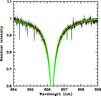
Figure 13: Example of fits to the H$\alpha$ line of the star BS 16023-043. The best-fit profile corresponds to $T_{\rm eff}$ = 6364 K. The other two profiles shown correspond to $T_{\rm eff}$ $\pm 200$ K of this value. The narrow absorption features are $\mathrm{H_{2}O}$ telluric lines.

This appendix is devoted to a detailed comparison of the temperature and metallicity scales of Asplund et al. (2006, , hereafter A06) and the ones derived in the present paper. Since there are no stars in common among the two studies we downloaded UVES spectra for two of the most metal-poor stars of A06 from the ESO archive: LP 815-43 and CD –33 1173. The list of spectra is given in Table A and includes all of the data used by A06, taken with the image slicer, as well as other data taken with the slit and more similar to our LP data. The purpose of this exercise is to compare data reduction and analysis procedures. An example of an H$\alpha$ fit for one of our program stars is given in Fig. 13.

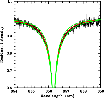
Figure 14: The H$\alpha$ profile of LP 815-043. The upper profile is from the 2004 slicer data, while the lower profile is from the 2001 slit data. It is clear that the slicer profile is distorted.

Our data reduction procedure includes division by a normalized flat-field, which achieves a correction of both the detector pixel-to-pixel variations and the echelle blaze function. The blaze function pattern is removed at the level of a few percent in our slit spectra, which is sufficient to obtain reliable profile of H$\alpha$, as shown in Fig. 13. The procedure fails on the data taken with image slicer # 3, as shown in Fig. 14, which compares a spectrum of star LP 815-43 taken with the image slicer with another spectrum taken without the image slicer. The blaze profile of the stellar spectrum (taken through the image slicer) appears significantly different from that of the flat-field spectrum (which is taken without the slicer, through a slit). The reduction procedure adopted by A06 differs from ours in that the blaze function is approximated by a polynomial fit directly on the stellar spectrum (the spectra of metal-poor stars are line-free enough to make this procedure unambiguous), and for the order containing H$\alpha$ for which this is impossible, the blaze profile is obtained by interpolating between the profiles of the two adjacent orders. Clearly, if we adopted the same procedure we would obtain results identical, or at least very similar ones to those of A06; however, this would not tell us much about the similarity of the two temperature scales.

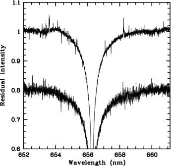
Figure 15: Example of fits to the H$\alpha$ line of the star LP 815-043, based on the 2001 slit data. The best-fit profile corresponds to $T_{\rm eff}$ = 6409 K, while the other two profiles shown correspond to $T_{\rm eff}$ $\pm 200$ K of this value.

Instead we preferred to use the slit data that was available for the two stars and that is very similar to our LP data. For star LP 815-43, from one spectrum we obtain $T_{\rm eff}$ = 6364 K and for the other $T_{\rm eff}$ = 6409 K, the mean is 6387 K, to be compared with 6400 K of A06 i.e. 13 K cooler. For CD –33 1173 we have 6 spectra, the mean $T_{\rm eff}$ is 6326 K with a standard deviation of 34 K, to be compared with $T_{\rm eff}$ = 6390 K of A06, i.e., 64 K cooler. The average of these two differences is $\sim 38$K. This is considerably smaller than our estimate of the error on $T_{\rm eff}$ . Therefore our interpretation is that our temperatures and those of A06 are on the same scale, although a zero point shift of up to $\sim 40$K is possible.

The comparison of the metallicities scale requires more effort and was therefore done only for LP 815-43. We used the spectra in Table A to measure the equivalent widths of the Fe i and Fe ii lines that have been used for all of our programme stars. These have been used, together with our model atmospheres with the $T_{\rm eff}$ = 6400, as input to the turbospectrum code to determine the abundances. The surface gravity and microturbulent velocity were iteratively adjusted to attain iron ionization equilibrium and independence of abundance from equivalent width. Our final parameters for this star are [Fe/H]=-2.94 log g = 3.90 and $\xi=1.61$ ${\rm km\,s}^{-1}$ . The line by line results are given in Table A. We note that our gravity is consistent, within errors with the gravity of A06 (log g = 4.17), which is derived from Strömgren photometry for this star and therefore has an error of $\sim 0.25$dex, like our own. We therefore conclude that the A06 metallicity scale over-estimates [Fe/H] by 0.2 dex and apply this rigid shift to all of his data.

[x]llllll Archive data for LP 815-43 and CD –33 1173

Star Date $t_{exp}$(s) $\lambda_{c}$ (nm) Slit MJD-24000.5

continued.

Star Date $t_{exp}$(s) $\lambda_{c}$ (nm) Slit MJD-24000.5

LP 815-43 1999-10-16 5400 346 0$\aas@@fstack{\prime\prime}$8 51467.018148000
1999-10-16 2700 346 1$\aas@@fstack{\prime\prime}$0 51459.008923800
2000-07-24 1800 705 SLIC# 3 51749.164882190
2000-07-24 1800 705 SLIC# 3 51749.186416570
2000-07-25 1200 705 SLIC# 3 51750.211278810
2000-07-25 1200 705 SLIC# 3 51750.225785770
2001-06-06 1200 437 0$\aas@@fstack{\prime\prime}$7 52066.366975750
2001-06-06 1200 437 0$\aas@@fstack{\prime\prime}$7 52066.381358710
2001-06-06 1200 437 0$\aas@@fstack{\prime\prime}$7 52066.395742820
2001-11-26 300 580 0$\aas@@fstack{\prime\prime}$8 52239.029463940
2001-11-26 600 580 0$\aas@@fstack{\prime\prime}$8 52240.015000550
2004-08-30 3000 600 SLIC# 3 53247.147858160
2004-08-30 3000 600 SLIC# 3 53247.185733820
2004-08-30 3000 600 SLIC# 3 53247.222292000
2004-08-31 3000 600 SLIC# 3 53248.011494530
2004-08-31 3000 600 SLIC# 3 53248.048641650
2004-08-31 3000 600 SLIC# 3 53248.184532180
CD –33 1173 2002-01-12 1500 580 0$\aas@@fstack{\prime\prime}$9 52286.045541490
2002-01-12 1500 580 0$\aas@@fstack{\prime\prime}$9 52286.063493190
2002-01-12 1500 580 0$\aas@@fstack{\prime\prime}$9 52286.081448180
2002-01-12 1500 580 0$\aas@@fstack{\prime\prime}$9 52286.102812080
2002-01-12 1500 580 0$\aas@@fstack{\prime\prime}$9 52286.120760860
2002-01-12 1500 580 0$\aas@@fstack{\prime\prime}$9 52286.138718950
2002-02-06 1800 705 SLIC# 3 52311.017325910
2002-02-06 1800 705 SLIC# 3 52311.039937800
2002-02-06 1800 705 SLIC# 3 52311.062072870

[x]llllll Equivalent widths of iron lines and abundances

LP 815-43
$\lambda$ $\chi$ log gf Ref. EW A(Fe)
nm eV pm dex

continued.

LP 815-43
$\lambda$ $\chi$ log gf Ref. EW A(Fe)
nm eV pm dex

Fe i
335.5228 3.30 $-0.405$ BWL 0.28 4.62
337.0783 2.69 $-0.266$ BWL 0.86 4.46
339.9333 2.20 $-0.622$ BWL 1.18 4.53
340.1519 0.92 $-2.059$ BWL 0.48 4.37
340.7460 2.18 $-0.020$ BWL 2.95 4.46
341.3132 2.20 $-0.404$ BWL 1.66 4.49
341.7841 2.22 $-0.676$ BWL 1.11 4.57
341.8507 2.22 $-0.761$ BWL 0.81 4.50
342.4284 2.18 $-0.703$ BWL 0.98 4.49
342.5010 3.05 $-0.500$ BWL 0.38 4.62
342.6383 0.99 $-1.909$ BWL 0.68 4.45
342.7119 2.18 $-0.098$ BWL 2.90 4.52
342.8193 2.20 $-0.822$ BWL 0.77 4.51
344.0606 0.00 $-0.673$ BWL 8.13 4.67
344.0989 0.05 $-0.958$ BWL 7.13 4.66
344.3876 0.09 $-1.374$ BWL 5.45 4.55
344.5149 2.20 $-0.535$ BWL 1.30 4.49
344.7278 2.20 $-1.021$ BWL 0.40 4.40
345.0328 2.22 $+0.902$ BWL 0.52 4.43
345.2275 0.96 $-1.919$ BWL 0.89 4.56
347.5450 0.09 $-1.054$ BWL 6.73 4.64
347.6702 0.12 $-1.507$ BWL 5.00 4.59
348.5340 2.20 $-1.149$ BWL 0.40 4.53
349.0574 0.05 $-1.105$ BWL 6.67 4.64
349.7841 0.11 $-1.549$ BWL 4.93 4.60
352.1261 0.92 $-0.988$ BWL 3.96 4.52
353.3198 2.88 $-0.112$ BWL 1.65 4.80
353.6556 2.88 $+0.115$ BWL 1.42 4.49
354.1083 2.85 $+0.252$ BWL 1.75 4.45
354.2076 2.87 $+0.207$ BWL 1.72 4.49
355.3739 3.57 $+0.269$ BWL 0.68 4.59
355.4118 0.96 $-2.206$ BWL 0.42 4.48
355.4925 2.83 $+0.538$ BWL 2.75 4.43
355.6878 2.85 $-0.040$ FMW 2.04 4.83
356.5379 0.96 $-0.133$ BWL 6.80 4.51
358.1193 0.86 $+0.406$ FMW 9.22 4.62
358.4659 2.69 $-0.157$ BWL 1.82 4.73
358.5319 0.96 $-0.802$ BWL 5.20 4.69
358.5705 0.92 $-1.187$ FMW 3.49 4.60
358.6113 3.24 $+0.173$ BWL 1.08 4.61
358.9105 0.86 $-2.115$ FMW 1.04 4.73
360.3204 2.69 $-0.256$ BWL 0.99 4.51
360.6679 2.69 $+0.323$ BWL 2.73 4.51
360.8859 1.01 $-0.100$ FMW 6.80 4.52
361.0159 2.81 $+0.176$ BWL 2.49 4.70
361.7786 3.02 $-0.029$ BWL+BK 0.90 4.52
361.8768 0.99 $-0.003$ BWL 7.16 4.52
362.2003 2.76 $-0.150$ BWL 1.03 4.48
362.3186 2.40 $-0.767$ BWL 0.58 4.50
363.8296 2.76 $-0.375$ BWL 0.71 4.52
364.0389 2.73 $-0.107$ BWL 1.26 4.51
380.5343 3.30 $+0.312$ BWL 1.39 4.48
380.6696 3.27 $+0.017$ BWL 0.96 4.56
380.7537 2.22 $-0.992$ BWL 0.69 4.49
381.5840 1.49 $+0.237$ BWL 7.99 4.57
382.0425 0.86 $+0.119$ FMW 9.79 4.63
382.1178 3.27 $+0.198$ BWL 1.38 4.56
382.5881 0.92 $-0.037$ FMW 8.29 4.43
382.7823 1.56 $+0.062$ FMW 6.14 4.32
384.0438 0.99 $-0.506$ FMW 6.08 4.36
384.3257 3.05 $-0.241$ BWL 0.72 4.48
384.9967 1.01 $-0.871$ FMW 5.27 4.56
385.0818 0.99 $-1.734$ FMW 1.73 4.59
385.2573 2.18 $-1.185$ BWL 0.54 4.53
385.6372 0.05 $-1.286$ FMW 7.53 4.70
385.9213 2.40 $-0.749$ BWL 1.00 4.58
385.9911 0.00 $-0.710$ FMW 9.83 4.75
386.5523 1.01 $-0.982$ FMW 5.05 4.62
386.7216 3.02 $-0.451$ BWL 0.65 4.62
387.2501 0.99 $-0.928$ FMW 4.99 4.53
387.8018 0.96 $-0.914$ FMW 5.31 4.56
389.5656 0.11 $-1.670$ FMW 4.66 4.40
389.9707 0.09 $-1.531$ FMW 5.81 4.50
390.2946 1.56 $-0.466$ FMW 4.69 4.51
390.6480 0.11 $-2.243$ FMW 2.59 4.53
391.7181 0.99 $-2.155$ FMW 0.89 4.66
392.0258 0.12 $-1.746$ FMW 5.29 4.62
392.7920 0.11 $-1.522$ BWL 6.34 4.64
394.0878 0.96 $-2.600$ FMW 0.29 4.56
395.6677 2.69 $-0.429$ BWL 1.11 4.56
399.7392 2.73 $-0.479$ BWL 1.16 4.66
400.5242 1.56 $-0.610$ FMW 4.55 4.61
400.9713 2.22 $-1.252$ BWL 0.47 4.55
401.4531 3.05 $-0.587$ BWL 0.47 4.62
402.1867 2.76 $-0.729$ BWL 0.55 4.58
404.5812 1.49 $+0.280$ FMW 8.03 4.49
406.3594 1.56 $+0.062$ BWL 7.19 4.55
407.1738 1.61 $-0.022$ FMW 6.56 4.51
413.2058 1.61 $-0.675$ BWL 3.99 4.59
413.4678 2.83 $-0.649$ BWL 0.80 4.73
414.3415 3.05 $-0.204$ BWL 1.17 4.66
414.3868 1.56 $-0.511$ BWL 5.12 4.62
418.1755 2.83 $-0.371$ BWL 1.43 4.74
418.7039 2.45 $-0.548$ FMW 1.50 4.60
418.7795 2.42 $-0.554$ FMW 1.49 4.58
419.1431 2.47 $-0.666$ BWL 1.05 4.55
419.8304 2.40 $-0.719$ FMW 1.64 4.77
419.9095 3.05 $+0.155$ BWL 2.29 4.66
420.2029 1.49 $-0.708$ FMW 4.59 4.63
421.0344 2.48 $-0.928$ BWL 0.68 4.62
421.6184 0.00 $-3.356$ FMW 0.55 4.71
421.9360 3.57 $+0.000$ BWL 0.61 4.60
422.2213 2.45 $-0.967$ FMW 0.65 4.61
422.7427 3.33 $+0.266$ BWL 1.74 4.64
423.3603 2.48 $-0.604$ FMW 1.40 4.64
423.5937 2.42 $-0.341$ FMW 2.13 4.56
425.0119 2.47 $-0.405$ FMW 1.93 4.60
425.0787 1.56 $-0.714$ BWL 4.01 4.58
426.0474 2.40 $+0.109$ BWL+BK 4.12 4.52
427.1154 2.45 $-0.349$ FMW 2.15 4.59
427.1761 1.49 $-0.164$ FMW 7.09 4.65
428.2403 2.18 $-0.779$ BWL 1.60 4.62
429.9235 2.42 $-0.405$ BWL 2.14 4.62
432.5762 1.61 $+0.006$ BWL 6.97 4.56
435.2735 2.22 $-1.287$ BWL 0.53 4.62
437.5930 0.00 $-3.031$ FMW 1.03 4.67
438.3545 1.49 $+0.200$ FMW 8.64 4.68
440.4750 1.56 $-0.142$ FMW 6.44 4.52
441.5123 1.61 $-0.615$ FMW 4.36 4.59
442.7310 0.05 $-2.924$ BWL 1.02 4.61
444.2339 2.20 $-1.255$ FMW 0.54 4.57
445.9118 2.18 $-1.279$ FMW 0.57 4.60
446.1653 0.09 $-3.210$ FMW 0.62 4.68
448.2170 0.11 $-3.501$ FMW 0.48 4.87
449.4563 2.20 $-1.136$ FMW 0.73 4.59
452.8614 2.18 $-0.822$ FMW 1.42 4.58
487.1318 2.87 $-0.363$ BWL 1.02 4.55
487.2138 2.88 $-0.567$ BWL 0.67 4.57
489.0755 2.88 $-0.394$ BWL 0.97 4.56
489.1492 2.85 $-0.112$ BWL 1.68 4.54
491.8994 2.87 $-0.342$ BWL 1.13 4.58
492.0503 2.83 $+0.068$ BWL 2.37 4.53
495.7597 2.81 $+0.233$ BWL 3.27 4.55
Fe ii
423.3172 2.58 $-1.900$ av 2.06 4.65
492.3927 2.89 $-1.320$ av 3.21 4.58

References

- Bard et al. (1991) Bard, A., Kock, A., & Kock, M. 1991, A&A, 248, 315 (BKK)
- Bridges (1973) Bridges, J. M. 1973, Phenomena in Ionized Gases, Eleventh International Conference, 418 (B)
- (3) Fuhr, J.R., Martin, G.A., and Wiese, W.L. 1988 Journal of Physical and Chemical Reference Data, 17, Suppl. 4 (FMW)
- O’Brian et al. (1991) O’Brian, T. R., Wickliffe, M. E., Lawler, J. E., Whaling, W., & Brault, J. W. 1991, Journal of the Optical Society of America B: Optical Physics, Volume 8, Issue 6, June 1991, pp.1185-1201, 8, 1185 (BWL)