Midplane sedimentation of large solid bodies in turbulent protoplanetary discs

Abstract

We study the vertical settling of solid bodies in a turbulent protoplanetary disc. We consider the situation when the coupling to the gas is weak or equivalently when the particle stopping time $\tau_{st}$ due to friction with the gas is long compared to the orbital timescale $\Omega^{-1}$. An analytical model, which takes into account the stochastic nature of the sedimentation process using a Fokker-Planck equation for the particle distribution function in phase space, is used to obtain the vertical scale height of the solid layer as a function of the vertical component of the turbulent gas velocity correlation function and the particle stopping time. This is found to be of the same form as the relation obtained for strongly coupled particles in previous work.

We compare the predictions of this model with results obtained from local shearing box MHD simulations of solid particles embedded in a vertically stratified disc in which there is turbulence driven by the MRI. We find that the ratio of the dust disc thickness to the gas disc thickness satifies $H_{d}/H=0.08(\Omega\tau_{st})^{-1/2}$, which is in very good agreement with the analytical model. By discussing the conditions for gravitational instability in the outer regions of protoplanetary discs in which there is a similar level of turbulence, we find that bodies in the size range $50$ to $600$ metres can aggregate to form Kuiper belt–like objects with characteristic radii ranging from tens to hundreds of kilometres.

1 Introduction

Dust is the constituent of planetesimals, that are believed to lead to the formation of planets in our own and other solar systems. Observational evidence for growth of dust particles in protoplanetary discs comes from near and mid-infrared imaging, mid-infrared spectrometry and millimetre interferometry (Natta et al., 2006; Rodmann et al., 2006). They point to the presence of grains of millimetre and even centimeter size in discs around clasical T Tauri stars.

In laminar discs, it is well known that gas drag causes the particles to sediment towards the disc midplane. In the absence of turbulence, there is nothing to oppose sedimentation and a very thin dust sub–layer can form. Thus there is a possibility that gravitational instability ocurs giving rise to gravitationally bound clumps, eventually leading to planetesimal formation (Goldreich & Ward, 1973). But collective effects arising through the interaction of the optically thick sedimenting dust layer with the gas may lead to the generation of turbulence and inhibit gravitational instability (see for example Weidenschilling, 1980; Cuzzi et al., 1993; Youdin & Shu, 2002; Gómez & Ostriker, 2005).

On the other hand, provided an adequate degree of ionisation can be maintained, accretion flows in which the dominant motion is Keplerian rotation, such as occur in protoplanetary discs, are not laminar. They have been shown to develop turbulence as a result of the magnetorotational instability (MRI; Hawley et al., 1995). The gaseous velocity fluctuations associated with the turbulence affect the spatial distribution of particles. Small particles are strongly coupled to the fluid and essentially follow the gas.

The radial diffusion of a passive contaminant was studied by Carballido et al. (2005), who found a diffusion coefficient approximately 10 times smaller than the effective disc kinematic viscosity associated with angular momentum transport. As shown recently by Johansen et al. (2006), this ratio, found to be of order unity in other simulations (Johansen & Klahr, 2005), is dependent on the topology of the initial magnetic field and the amount of conserved magnetic flux present, which determines the level of the resulting turbulence. They note that the form of the particle diffusion induced by the turbulence is apparently determined by this level, or equivalently, the amount of angular momentum transport. Turner et al. (2006) also studied the vertical spreading of a trace species in the upper layers of a stratified disc. They found radial spreading to be faster than vertical spreading throughout the vertical extent of the disc.

Larger particles, for which the coupling is weaker, are found to start to sediment despite the presence of turbulence. For a surface density $\Sigma=200$ g cm^-2 being characteristic of the minimum mass solar nebula at $5.2$ AU, sedimentation was found to begin for particle sizes between a centimetre and a metre in a disc model with MRI driven turbulence (Fromang & Papaloizou, 2006, hereafter FP). FP modelled this settling process by means of an advection-diffusion equation for the dust density. They expressed the diffusion coefficient in terms of the turbulent gas velocity correlation function. They found that turbulence stirs the dust sub-layer significantly, up to approximately 20% of the disc scale height for particles of about 10 cm in radius at $5.2$ AU. Thus dust particles of this size range could not be the constituents of a gravitationally unstable sub-disc. Accordingly, on a scale of $5$ AU in a minimum mass solar nebula, the formation of planetesimals is hindered until a much larger particle size range is reached when the MRI operates.

The above studies modelled the dust component as a second fluid. However, to study the effect of MHD turbulence on solids of larger size such that the stopping time due to gas drag significantly exceeds the inverse orbital angular frequency, it is necessary to model dust grains as discrete particles. Johansen et al. (2006) have performed local three-dimensional simulations of a non-stratified turbulent protoplanetary disc and find that individual particles tend to concentrate by a factor of up to 100 due to radial concentration in vortices. They suggest that such dust agglomerations can potentially become gravitationally unstable. However, their study did not address the effect of the vertical sedimentation of solid bodies.

It is the purpose of this paper to perform a study of the stochastic vertical settling of solids that is applicable when the stopping time is much larger than the orbital period. Firstly we develop an analytical model based on solving a one dimensional Fokker–Planck equation. The derivation of this equation and its solution are presented in Section 2. This gives an expression for the dust sub–disc thickness as a function of particle size. In Section 3, we go on to compare these results, and others found in previous work applicable to strongly coupled small particles, with those found from simulations of solid particles embedded in a turbulent protoplanetary disc. Simulations have been performed which treat the dust dynamics using the Epstein and Stokes drag laws (Weidenschilling, 1977). Note that these include locally induced radial motion, but not that induced by a global radial pressure gardient, so that in the former context, the vertical settling that is found will occur regardless of radial concentration in vortices as long as the particles do not collide. Finally, in Section 4 we discuss the implications of our results for the formation of planetesimals and the possibility of gravitational instability in the outer regions of protoplanetary discs.

2 The model

In a protoplanetary disc, solid bodies evolve under the combined influence of gas drag and MHD turbulence. By damping motion relative to the gas, on average the former results in settling towards the equatorial plane of the disc. Simultaneously, the latter excites random motions that oppose the settling process. The ensemble of solid bodies will eventually reach a steady state with an associated vertical semi-thickness $H_{d}$. Below we present a model to determine this equilibrium state which is applicable when the coupling of the particle to the gas is weak and such that the stopping time is very much longer than the orbital period.

2.1 Definitions and notation

The interaction between the gas and the solid bodies (dust, boulders, planetesimals) occurs through a drag force $F_{D}$. This can be written as

$$\mbox{\boldmath{$F_{D}$}}=m_{p}\frac{\mbox{\boldmath{$u$}}-\mbox{\boldmath{$v$}}}{\tau_{\rm{st}}}\,,$$ (1)

where $m_{p}$ is the mass of a particle, $v$ its velocity and $u$ is the gas velocity.

The characteristic time required to equilibrate gas and particle velocities, or stopping time is $\tau_{\rm{st}}.$ This depends on the ratio of the size of the particle, expressed through the radius $a$ they would have if they were spherical, and the mean free path of the gas molecules, $\lambda$ (Weidenschilling, 1977; Cuzzi et al., 1993). When $\lambda>(4/9)a$, we are in the Epstein regime for which

$$\tau^{(Ep)}_{\rm{st}}=\frac{\rho_{s}}{\rho}\frac{a}{c_{s}}\,,$$ (2)

where $\rho_{s}$ is the solid mass density and $c_{s}$ is the gas speed of sound.

When $\lambda<(4/9)a$, we are in the Stokes regime, and $\tau^{(St)}_{\rm{st}}$ is defined through

$$\tau^{(St)}_{\rm{st}}=\frac{8}{3}\frac{\rho_{s}}{\rho}\frac{a}{C_{D}|\mbox{\boldmath{$u$}}-\mbox{\boldmath{$v$}}|}\,,$$ (3)

where $C_{D}$ is a dimensionless coefficient that depends on the Reynolds number of the flow ${\cal R}_{e},$ tending to a constant value of order unity for ${\cal R}_{e}\rightarrow\infty.$

2.2 Diffusion in velocity–space

Since we are interested in the problem of vertical settling, we restrict the analysis to consider only the vertical direction $z,$ though we shall consider relevant results of simulations relating to the horizontal directions below.

The vertical component of the equation of motion for a single particle moving under the gravitational acceleration due to the central star and gas drag can be written as

$$\frac{dv_{z}}{dt}=-\Omega^{2}z+\frac{u_{z}-v_{z}}{\tau_{\rm{st}}}$$ (4)

where $u_{z}$ is the vertical component of the gas velocity which is fluctuating stochastically because it is turbulent. Below we make the approximation that $\tau_{\rm{st}}$ is constant. In reality, in the Epstein regime, density fluctuations will cause $\tau^{(Ep)}_{\rm{st}}$ to vary with time. In the Stokes regime, both density and velocity fluctuations will have the same effect. However, we expect the essential physics to be retained if we adopt an appropriate time averaged value of $\tau_{\rm{st}},$ so we assume this to have been done in what follows.

Equation (4) can be written as an equation for a damped harmonic oscillator randomly forced in time by the part of the drag force proportional to the gaseous turbulent velocity field:

$$\frac{dv_{z}}{dt}+\frac{v_{z}}{\tau_{\rm{st}}}+\Omega^{2}z=\frac{u_{z}}{\tau_{\rm{st}}}\equiv F\,.$$ (5)

The particle motion can be regarded as driven by the stochasting forcing term $F$. When the correlation time of the gas velocity is much smaller than the orbital period, this can be regarded as producing a series of weak (which will be the case when the stopping time is large) random impulsive changes to the velocity of the particle. FP found that the correlation time of the turbulent eddies is typically $0.15$ orbits, which marginally satifies this condition. Nonetheless we proceed with the model and later compare with simulation results. In a time interval $(t_{0},t)$, the change $\delta v_{z}$ of the particle velocity produced by the random acceleration $F$ can be written as

$$\delta v_{z}=\int_{t_{0}}^{t}Fdt^{\prime}=\int_{t_{0}}^{t}\frac{u_{z}(z,t^{\prime})}{\tau_{\rm{st}}}dt^{\prime}\,.$$ (6)

Because of the stochastic nature of $F$, this reduces to zero when a suitable ensemble average is taken: $\langle\delta v_{z}\rangle$=0. To describe the evolution of the particle distribution, we need to calculate the mean square deviation of the particle velocity:

$$\frac{1}{2}\left(\frac{d\,\left(\delta v_{z}\right)^{2}}{dt}\right)=\int_{t_{0}}^{t}\frac{u_{z}(z,t)u_{z}(z,t^{\prime})}{\tau_{\rm{st}}^{2}}dt^{\prime}$$ (7)

Now, we take an ensemble average. When this is done, for an assumed steady state and local homogeneous turbulence, the result of the integral depends only on the time difference $t-t^{\prime}$. Furthermore, there is no prefered time so we finally get

$$\frac{d\,\langle\left(\delta v_{z}\right)^{2}\rangle}{dt}=\frac{2}{\tau_{\rm{st}}^{2}}\int_{0}^{t}\langle u_{z}(z,t)u_{z}(z,0)\rangle dt=\frac{2}{\tau_{\rm{st}}^{2}}\int_{0}^{t}S_{zz}(t)dt.$$ (8)

Here $S_{zz}(t)$ is the velocity correlation function used in FP where the reader is referred for more discussion of the above aspects. At large times, we thus obtain the limiting form

$$\frac{d\,\langle\left(\delta v_{z}\right)^{2}\rangle}{dt}\to\frac{2D_{{\rm T}}(\infty)}{\tau_{\rm{st}}^{2}}$$ (9)

where $D_{\rm T}(\infty)\equiv\int_{0}^{\infty}\langle u_{z}(z,\Delta t)u_{z}(z,0)\rangle d(\Delta t)$ defines an effective diffusion coefficient and was already used by FP in a different context in their discussion of small particles well coupled to the gas, where it is the spatial diffusion coefficient. Integrating the last equation, we finally obtain for large time $t$

$$\langle(\delta v_{z})^{2}\rangle\sim\frac{2D_{\rm T}(\infty)t}{\tau_{\rm{st}}^{2}}$$ (10)

The linear dependence in time in this expression shows that the particles experience a random walk in velocity space, with an effective diffusion coefficient

$$D_{\rm{v}}=\frac{D_{\rm T}(\infty)}{\tau_{\rm{st}}^{2}}.$$ (11)

We comment that if we set $t\sim\tau_{\rm{st}}$ in equation (10), we expect that the mean square velocity dispersion ${\langle(\delta v_{z})^{2}}\rangle\sim 2D_{\rm T}(\infty)/\tau_{\rm{st}},$ a form found by Voelk et al. (1980) from considerations of stochastic forcing and a specific turbulence model.

2.3 Fokker–Planck equation

The next step is to determine the particle distribution function $f=f(z,v_{z},t)$, from which quantities such as the vertical semi-thickness can be determined. Its evolution in phase space can be described by the one-dimensional Fokker-Planck equation. For the system we study, the particles are subject to frictional drag and gravity due to the central star as written in equation (5) while their velocities diffuse in velocity space with diffusion coefficient $D_{\rm{v}}$ given by equation (10). Then, the Fokker–Planck equation takes the form (Chandrasekhar, 1949; Johnson et al., 2006):

$$\frac{\partial f}{\partial t}+v_{z}\frac{\partial f}{\partial z}+\frac{\partial}{\partial v_{z}}\left(bf\right)=D_{\rm{v}}\frac{\partial^{2}f}{\partial v_{z}^{2}},$$ (12)

where $b=-\Omega^{2}z-v_{z}/\tau_{\rm{st}}$ is the non-stochastic acceleration. The derivation of equation (12) is given in Appendix A.

We seek equilibrium solutions, expected to be attained on a time scale comparable to the stopping time, for the distribution function found by setting $\frac{\partial}{\partial t}=0$ in Eq. (12). We find a solution for $f$ of the form

$$f(z,v_{z})\propto e^{-\beta\left(\frac{v_{z}^{2}}{2}+\frac{\Omega^{2}z^{2}}{2}\right)},$$ (13)

where

$$\beta=\frac{\tau_{\rm{st}}}{D_{{\rm T}}(\infty)}.$$ (14)

Thus the thickness of the solid body layer $H_{d}$ is written as

$$H_{d}=\sqrt{\frac{D_{{\rm T}}(\infty)}{\tau_{\rm{st}}\Omega^{2}}}.$$ (15)

We note that this form of $H_{d}$ as the parameter of a Gaussian distribution in $z$ is of the same from as applies to the strongly coupled small particle case (see Dubrulle et al., 1995, or FP). Thus the expression properly extends to all particle sizes.

3 Numerical simulations

In this section, we present a set of numerical simulations that confirm the results of the discussion above. Those are local simulations of stratified discs that use the shearing sheet approximation (Hawley et al., 1995; Stone et al., 1996). The disc becomes turbulent in the presence of a weak magnetic field. When turbulence is well established, we follow the evolution of dust particles and larger solid bodies using two different algorithms and compare the steady–state thickness of the solid layer to the results presented above. Below, we describe the set–up of the simulations before going on to give our results.

3.1 Method

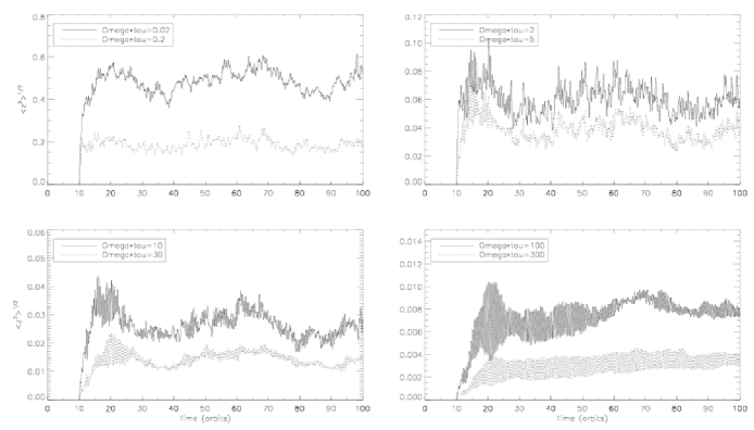
Figure 1: Root mean square vertical displacement as a function of time for the couplings $\Omega\tau_{\rm{st}}=0.02$, $0.2$, $2$, $5$, $10$, $30$, $100$ and $300$ (given at the upper left hand corner of each plot). Note the different scale used on each plot.

We used the ZEUS code (Stone & Norman, 1992a, b) to evolve the standard MHD equations in a shearing box (Goldreich & Lynden-Bell, 1965). For the gas, we used a set–up identical to that described in FP. In standard Cartesian coordinates $(x,y,z)$, the box has a size $(H,2\pi H,6H)$ and we use a resolution $(N_{x},N_{y},N_{z})=(32,100,196)$. We comment that the shearing box represents a local patch of a differentially rotating disc and has been used by many authors (eg. Hawley et al., 1995; Stone et al., 1996, FP) for the purposes of simulating MHD turbulence. The coordinate origin is at the centre of the box with the $x$ and $y$ axes pointing in the outward radial direction and the direction of rotation respectively. The length scale is $H,$ the time scale is set by $\Omega^{-1},$ and mass scale is determined by the gas density scale. Here the self–gravity of the gas is neglected. There is no information concerning the distance to the centre of the disc other than it should be much larger than $H.$ However, the shearing box can be thought of as providing a detailed representation of a local region of a disc for which $H$ and the distance to the centre are determined by global considerations.

In our simulations, the equation of state is isothermal. The disc, initially in hydrostatic equilibrium in the vertical direction, is threaded by a magnetic field with zero net flux, such that the ratio of thermal to volume averaged magnetic pressure, $\beta,$ is equal to 400. Because of the MRI, MHD turbulence develops and is maintained for at least $100$ orbits. In agreement with previous published results (Stone et al., 1996), we found that $\alpha$, the ratio of the volume averaged total stress (the sum of the $(x,y)$ components of the Maxwell and Reynolds stress tensors) to $P_{0},$ which governs the angular nomentum transport, is typically $0.015$ throughout this type of simulation (see FP for details).

This model was then used as a basis to investigate the evolution of an ensemble of solids of different sizes. To do so, we used two different algorithms. First, we adopted an N–body approach well suited to the bodies of large size that we want to consider. In that case, the velocities and positions of individual particles are updated in two steps: the gas velocities are first interpolated at the position of the particles using a bilinear interpolation method. Then, a second order Runge–Kutta method is used to update the velocities and positions of the particles in time according to their equation of motion. For the smallest particles that we studied, we also used the two–fluid algorithm presented by FP, in which the dust component is modelled as a second pressureless fluid. In both cases, neither the back reaction of the particles on the gas nor inter-particle interactions are included.

The N–body approach was used to investigate the evolution of solid bodies of $8$ different sizes. In each case, the particles were assumed to be in the Epstein regime, so that $\tau_{\rm{st}}$ is evaluated according to equation (2). To label the model, we used the value of the dimensionless parameter $\Omega\tau_{\rm{st}}$, where $\tau_{\rm{st}}$ is evaluated in the midplane of the unperturbed disc (i.e. the value of the density is that given by the hydrostatic equilibrium). Following this convention, the $8$ models we ran correspond to $\Omega\tau_{\rm{st}}=0.02$, $0.2$, $2$, $5$, $10$, $30$, $100$ and $300$. At $t=10$ orbits, we introduce $100$ particles for each of the models described above. They are distributed in the midplane of the disc where they form a horizontal lattice consisting of 25 columns and 4 rows of particles. Their initial velocities are set equal to zero. The system is then evolved for a further $90$ orbits. This long time integration enables a good sampling of the flow properties for each particle. This is why a larger number of particles is not required. Instead, we find that time–averaging the results over the duration of the runs provides a suitable statistical representation of the effect of MHD turbulence on the particle distribution.

In addition, two runs were performed with the two–fluid method mentioned above. They are limited to $\Omega\tau_{\rm{st}}=0.02$ and $0.2$ (indeed, in order for the two–fluid approach to be valid, we require $\Omega\tau_{\rm st}<1$). As for the N–body calculation, we assume that the Epstein law applies. The set–up we used for these two–fluid models is identical to that of FP: at $t=20$ orbits, the dust particles form a Gaussian thin disc such that $H_{d}=0.2H$ and their evolution is then followed for $80$ orbits.

3.2 Results

The results of the $8$ models that use the N–body approach are illustrated in figure 1. For each of them, a curve is plotted that shows the variations of the averaged root mean square displacement $\langle Z^{2}\rangle^{1/2}$ over all the particles with time. The value of $\Omega\tau_{\rm{st}}$ corresponding to each case is given in the upper left hand corner of each plot. For convenience we adopt a system of units such that $H=1.$ However, note the different scales on the vertical axes of the four panels. In each model, $\langle Z^{2}\rangle^{1/2}$ first increases before oscillating aroung a mean value. This mean value represents the average planetesimal disc semi-thickness. It is quickly well defined for the smallest particles ($\Omega\tau_{\rm{st}}\leq 30$). For $\Omega\tau_{\rm{st}}=100$ and $300$, more time is required before reaching an equilibrium. This is because the interaction between the particles and the gas is very weak in that case ($\tau_{\rm{st}}=15$ and $45$ orbits respectively).

Figure 2: Vertical profile for the dust to gas ratio in the two models, $\Omega\tau_{\rm{st}}=0.02$ (solid line) and $0.2$ (dashed line), in which the solid component is treated as a pressureless fluid. Both curves are time averaged between $t=65$ and $t=85$ orbits. The dotted line is a Gaussian fit to the data, using a thickness $H_{d}=0.55$ and $0.18$ respectively.

The results of the models that use the two–fluid approach are illustrated in figure 2. This shows the vertical profile of the dust to gas mass density ratio, averaged in time between $t=65$ and $t=85$ orbits for the two models: $\Omega\tau_{\rm{st}}=0.02$ (solid line) and $\Omega\tau_{\rm{st}}=0.2$ (dashed line). The dotted curves show the function

$$\frac{\rho_{d}}{\rho}=\left(\frac{\rho_{d}}{\rho}\right)_{0}\exp\left(-\frac{z^{2}}{2H_{d}^{2}}\right)\,,$$ (16)

with $H_{d}/H=0.55$ and $0.18$ respectively. These give the equilibrium dust disc semi-thickness for these two models.

Figure 3: Root-mean-square vertical displacement as a function of dimensionless stopping time. The filled circles (Epstein drag) and the asterisks (Stokes drag) represent data from simulations of individual particles, while the two diamonds were obtained from calculations regarding the dust component as a fluid. The straight line represents the equation $\langle z^{2}\rangle^{1/2}=0.08\,(\Omega\tau_{\rm{st}})^{-1/2}$.

In Fig. 3, we summarize the results of all models by plotting the root mean square vertical extents as a function of $\Omega\tau_{\rm{st}}$. The filled circles correspond to the simulations performed with the N–body algorithm. They are obtained by averaging the root mean square deviation of the particles between $50$ and $100$ orbits. The two diamonds are the data obtained from the two-fluid calculations described above (the stars appearing in figure 3 are further discussed in the discussion section below). The straight line shows the equation

$$\langle z^{2}\rangle^{1/2}=0.08\,(\Omega\tau_{\rm{st}})^{-1/2}\,.$$ (17)

which is the best fit to the data. It is seen to fit nicely the results of the simulations. This is expected according to the discussion given in section 2. Indeed, using the relation $H=c_{s}/\Omega$, equation (15) can be expressed as

$$\frac{H_{d}}{H}=\sqrt{\frac{D_{\rm T}(\infty)}{c_{s}H}}(\Omega\tau_{\rm{st}})^{-1/2}\,.$$ (18)

From the correlation function of the turbulent velocities, FP found $D_{\rm T}(\infty)=5.5\times 10^{-3}c_{s}H$, which gives

$$\frac{H_{d}}{H}=7.4\times 10^{-2}(\Omega\tau_{\rm{st}})^{-1/2}\,.$$ (19)

This is in very good agreement with the results of the simulations given by equation (17), so validating the discussion presented in Section 2.

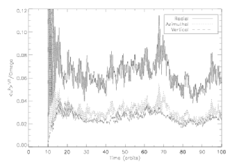
Figure 4: The form of the root mean square velocity components divided by $\Omega$ as a function of time for the particles with $\Omega\tau_{\rm{st}}=10.$ After initial transients, $\langle v_{x}^{2}\rangle^{1/2}\sim 2.5\langle v_{z}^{2}\rangle^{1/2}$ and $\langle v_{y}^{2}\rangle^{1/2}\sim 1.25\langle v_{z}^{2}\rangle^{1/2}.$ The $y$ component is measured relative to the local mean shear.

The evolution of $\langle v_{x}^{2}\rangle^{1/2},$ $\langle v_{y}^{2}\rangle^{1/2}$ and $\langle v_{z}^{2}\rangle^{1/2}$, being the the root mean square velocity components in the $x,y$ and $z$ directions, respectively, as a function of time is illustrated in figure 4 for the particles with $\Omega\tau_{\rm{st}}=10.$ Other values of the latter parameter give similar results. After initial transients, noting that the $y$ component is measured relative to the local mean shear, the ratios $\langle v_{y}^{2}\rangle^{1/2}/\langle v_{x}^{2}\rangle^{1/2}\sim 0.5$ and $\langle v_{z}^{2}\rangle^{1/2}/\langle v_{x}^{2}\rangle^{1/2}\sim 0.4$ are established. These can be understood as corresponding to the root mean square turbulent gas velocity components which show similar ratios (Hawley et al., 1995). In a shearing box simulation which reaches a quasi steady state such ratios are established and maintained. Restoring units, these velocity measures scale as $\Omega H.$

4 Discussion

We have presented an analytical estimate of the thickness of the solid layer formed by sedimenting solid bodies in a turbulent protoplanetary disc. The stochastic dust vertical displacement in the presence of turbulence is modelled using a Fokker-Planck equation, which describes the evolution of the particle distribution function in phase space. The steady state solution of this equation provides an expression for the thickness $H_{d}$ of the disc of solids. We found

$$H_{d}/H\propto(\Omega\tau_{\rm{st}})^{-1/2}\,.$$ (20)

To confirm this analytical result, we performed simulations of dust particles embedded in a vertically stratified and turbulent local model of a protoplanetary disc. We found the numerical values of the particle height dispersions to agree well with the Fokker-Planck result. These simulations were done utilising Epstein drag. In the following, we discuss the expected differences that will arise when Stokes drag is used.

4.1 The Stokes drag law

In the Stokes regime, the stopping time $\tau_{\rm{st}}$ is given by equation (3). For large particles, mostly confined in the vicinity of the equatorial plane, we should be in the regime in which $|\mbox{\boldmath{$v$}}|<<|\mbox{\boldmath{$u$}}|$. In that case, an averaged expression for the stopping time can be written as

$$\langle\tau_{\rm{st}}\rangle^{(St)}\sim\frac{8}{3C_{D}}\frac{\rho_{s}a}{\bar{\rho}c_{s}}\left(\frac{(\delta u_{z}^{2})^{1/2}}{c_{s}}\right)^{-1}\,,$$ (21)

where $\bar{\rho}$ is the mean value of the turbulent density field and $(\delta u_{z}^{2})^{1/2}$ is the root mean square turbulent gas vertical velocity fluctuation. We note that this expression gives a very naïve estimate of the average value of $\langle\tau_{\rm{st}}\rangle^{(St)}$. Indeed, $\tau_{\rm{st}}$, as defined in equation (3), depends on the turbulent velocity. As such, the theory developed in section 2.2 should be modified and thus higher order velocity correlations would appear. Such an analysis in detail is beyond the scope of this paper, but the replacement of the quadratic velocity dependence in the drag law by the product of a linear one and an average in the simple estimate is likely to underestimate the particle force fluctuations and accordingly underestimate the diffusion coefficient. As we will see below, however, such effects remain small. In equation (21), we have also considered $C_{\rm D}$ to be constant as in the large ${\cal R}_{e}$ limit. However, a dependence of $C_{\rm D}$ on $(\delta u_{z}^{2})^{1/2}$ could easily be incorporated.

Using equation (21), the dimensionless parameter $\langle\Omega\tau_{\rm{st}}\rangle^{(St)}$ can be written in terms of the dimensionless parameter $\langle\Omega\tau_{\rm{st}}\rangle^{(Ep)}$ corresponding to the Epstein regime, for which

$$\langle\Omega\tau_{\rm{st}}\rangle^{(Ep)}=\frac{\rho_{s}a}{\bar{\rho}c_{s}}\,.$$ (22)

Indeed, we have:

$$\langle\Omega\tau_{\rm{st}}\rangle^{(St)}=\frac{8}{3C_{D}}\langle\Omega\tau_{\rm{st}}\rangle^{(Ep)}\left(\frac{(\delta u_{z}^{2})^{1/2}}{c_{s}}\right)^{-1}\,.$$ (23)

In our numerical simulations, we found $(\delta u_{z}^{2})^{1/2}$ to be $\sim 0.13c_{s}$ in the disc midplane. This is in agreement with previous results (Stone et al., 1996; Turner et al., 2006). Furthermore, for the largest solid bodies, Weidenschilling (1977) gives $C_{D}=0.44$. In that case, equation (23) gives

$$\langle\Omega\tau_{\rm{st}}\rangle^{(St)}\sim 45\langle\Omega\tau_{\rm{st}}\rangle^{(Ep)}$$ (24)

This relation indicates that particles in the Stokes regime should behave similarly to particles in the Epstein regime, but with a value of the dimensionless parameter $\Omega\tau_{\rm{st}}$ that is $45$ times larger.

To check this, we performed two simulations in which the particles follow the Stokes drag law, with $C_{D}=0.44$, and we measured the equilibrium semi-thickness of the particle discs. The values of the dimensionless parameter $\langle\Omega\tau_{\rm{st}}\rangle^{(Ep)}$ for these runs were taken to be equal to $0.24$ and $2.4$ respectively. According to the discussion above, the effective dimensionless parameters $\langle\Omega\tau_{\rm{st}}\rangle^{(St)}$ are respectively $\sim 11$ and $\sim 110$. The measured particle disc thicknesses are represented in figure 3 with stars.

Although they lie close to the solid line (the vertical shift is between $50\%$ and a factor of 2), there seems to be a systematic difference with the Epstein results. This arises because, as we discussed above, the expression for the diffusion coefficient should be adjusted upwards. Because of the quadratic dependence on velocities of the drag force, we expect the points derived using the Stokes law to lie systematically above the equivalent Epstein points, as is observed in figure 3. Taking the limitations of the simple theory into account, the broad agreement of these simulations with the Epstein results is quite satisfactory and confirms our analysis.

4.2 Gravitational instability

Given the above results it is of interest to investigate whether gravitational instability of a sedimenting layer in a protoplanetary disc with the degree of turbulence considered here could be a possibility. We begin by remarking that studies of the degree of ionisation indicate that this may be adequate to allow the MRI to operate both at small distances $\lesssim 0.2$ AU and large distances $\gtrsim 10-50$ AU from the central star (Fromang et al., 2002), depending on the disc model. In the intermediate range, a dead zone is expected to be present and affect the results presented below. We will therefore concentrate on the outer parts of the disc in the following.

Weidenschilling (1994, ) has discussed the possible role of gravitational instability in the outer solar system in the formation of cometary aggregates. He considered bodies with $a\sim 10^{3-4}$ cm with a velocity dispersion determined by their radial drift driven by an underlying pressure gradient. Whether such large bodies may be formed through the aggregation of small particles is uncertain. Weidenschilling (1997) put forward a model applicable to a disc, without MHD turbulence, where bodies in this size range could aggregate by collisional sticking in the outer solar system on a $10^{5}$ year time scale. It is unclear to what extent the presence of MHD turbulence would extend this. The work described by Weidenschilling & Cuzzi (1993), appropriate to the inner solar system, indicates that the time scale may be extended by about an order of magnitude, in which case they could form within expected lifetimes of protostellar discs.

Here we shall assume that bodies in the $10^{4}$ cm size range can form and consider the effect of turbulence on the possibility of gravitational instability in the outer protoplanetary disc. In the first instance we neglect radial drift assuming that we are considering an ensemble of solids near a pressure maximum and return to this aspect later.

For the disc model, we adopt a surface density distribution as a function of radius $r$ that follows that of the minimum mass solar nebula (Hayashi et al., 1985). The surface density of the solid disc, $\sigma_{p}$, is given by

$$\sigma_{p}=\frac{\sigma_{0}}{\chi}\left(\frac{r}{5\textrm{AU}}\right)^{-3/2}\,,$$ (25)

where $\sigma_{0}$ is equal to 150 g.cm^-2 for the minimum mass solar nebula and $\chi$ is the gas to dust ratio. The optical depth of the disc of solids is

$$\tau=\frac{3\sigma_{p}}{4\rho_{s}a}.$$ (26)

For the surface density profile (25) this gives

$$\tau=\frac{3\sigma_{0}}{4\rho_{s}a\chi}\left(\frac{r}{5\textrm{AU}}\right)^{-3/2}.$$ (27)

Thus for $r\geq 5$ AU, and $a\gtrsim 1$ cm, the disc of solid material will be optically thin if we assume $\chi>100\left(r/5\textrm{AU}\right)^{-3/2}$. It will then not be able to act collectively as a fluid dust layer as in models that generate turbulence through interaction with the gas (eg. Goldreich & Ward, 1973; Weidenschilling, 1980).

Gravitational instability of the particle layer can occur if the Toomre (1964) criterion is satisfied:

$$\frac{c_{\rm{p}}\Omega}{\pi G\sigma_{\rm{p}}}<1\,,$$ (28)

where $c_{\rm{p}}$ is the particle velocity dispersion in the radial or $x$ direction and $G$ is the gravitational constant. The vertical scale height of the particle layer is $H_{\rm{d}}=\langle v_{z}^{2}\rangle^{1/2}/\Omega$. Because the turbulent velocity fluctuations are larger in the radial direction than in the azimutal and vertical directions, the induced root mean square velocity component fluctuations induced in the solid bodies exhibit the same ordering (see figure 4 and above). We found $\langle v_{x}^{2}\rangle^{1/2}\sim 2.5\langle v_{z}^{2}\rangle^{1/2}$ and $\langle v_{y}^{2}\rangle^{1/2}\sim 1.25\langle v_{z}^{2}\rangle^{1/2}.$ Thus $c_{\rm{p}}=\langle v_{x}^{2}\rangle^{1/2}\sim 2.5\langle v_{z}^{2}\rangle^{1/2}$. Equation (28) can then be expressed as

$${H_{d}\over r}<\frac{3.5\times 10^{-6}}{\chi}\left(\frac{r}{5\textrm{AU}}\right)^{1/2}\left(\frac{\sigma_{0}}{1\textrm{ g.cm}^{-2}}\right)\,,$$ (29)

where the mass of the central star has been taken equal to one solar mass and equation (25) has been used. Using Eq. (19), which gives the height of the dust layer determined by turbulent diffusion, we find that

$$\Omega\tau_{\rm{st}}>1.1\times 10^{6}\chi^{2}\left({H\over 0.05r}\right)^{2}\left(\frac{r}{5\rm{AU}}\right)^{-1}\left(\frac{\sigma_{0}}{1\textrm{ g.cm}^{-2}}\right)^{-2}\,.$$ (30)

Assuming the particles are in the Epstein regime (at $50$ AU, this is valid for particles smaller than approximately $1000$ metres) together with $\rho_{s}=2$ g.cm^-3, a condition on their size can be found from equation (2) in the form

$$a>2.8\chi^{2}\left({H\over 0.05r}\right)^{2}\left(\frac{r}{5\textrm{AU}}\right)^{-5/2}\left(\frac{\sigma_{0}}{1\textrm{ g.cm}^{-2}}\right)^{-1}\textrm{ km}\,.$$ (31)

Thus at 50 AU, for $H/r=0.05$, gravitational instability becomes possible for $a>600$ m for the minimum mass solar nebula if $\chi=100$. But note that this quantity decreases with both $\sigma_{0}$ and $r$ and increases with $\chi$. For example, in a disc of only $3$ times the minimum mass solar nebula, if $\chi=50$, solid boulders larger than $\sim 50$ metres will become gravitationally unstable at $50$ AU.

The length scale associated with the instability is $k^{-1}=H_{d},$ with a characteristic mass $M_{p}\sim 6\pi\sigma_{p}H_{\rm{d}}^{2}$ which gives

$$M_{p}\sim\frac{1.3\times 10^{18}}{\chi^{3}}\left(\frac{r}{5\textrm{AU}}\right)^{3/2}\left(\frac{\sigma_{0}}{1\textrm{ g.cm}^{-2}}\right)^{3}\textrm{g}\,,$$ (32)

corresponding to a solid body of radius $\sim 5.4(r/5\textrm{AU})^{1/2}\chi^{-1}(\sigma_{0}/1$g.cm^-2) km. At $50$ AU, for the minimum mass solar nebula and when $\chi=100$, this corresponds to a radius of $\sim 26$ km, similar to typical radii of Kuiper belt objects (Luu & Jewitt, 2002). In regions where $\sigma_{0}/\chi$ or equivalently solid surface density is locally enhanced, this size is accordingly increased. For example, for an an enhancement of a factor of $10$, the masses involved in the gravitational instability would correspond to bodies of $\sim 260$ km.

As noted by Weidenschilling (1995) this form of instability does not mean that gravitational collapse ensues but that a gravitationally bound cluster of total mass $M_{p}$ forms (see also Tanga et al., 2004). This then has to evolve through further settling and accumulation. Nevertheless, the analysis presented here shows that MHD turbulence does not necessarily prevent bodies of plausibly up to few $100$ km in radius forming by gravitational instability in the outer regions of protoplanetary discs.

Note that, in drawing this conclusion, we completely neglected the effect of radial migration and concentrated only on vertical settling. This is because, in general, the ratio of the radial drift speed to orbital speed, induced by a radial pressure gradient, being of order $(H/r)^{2}/(\Omega\tau_{\rm{st}})$ (see Papaloizou & Terquem, 2006, and references therein), is significantly less than $H_{d}/r$ near marginal stability for the conditions we consider, thus it can be safely neglected.

Appendix A The Fokker-Planck equation

The purpose of this appendix is to present a derivation of the Fokker–Planck equation (12) that we used in section 2 to estimate the planetesimal disc thickness. This derivation is largely based on Chandrasekhar (1949) in which applications of the theory of Brownian motion to dynamical friction and stellar dynamics are discussed.

Consider the motion of a given solid body in the vertical direction. During a small time $\Delta t$ , it will undergo a change in velocity $\Delta v_{z}$. Some of this change is due to stochastic forces that arise from the turbulent gas, and which have correlation times that are assumed to be smaller than the time required for typical velocities of the solid bodies to change significantly. Also velocity changes induced during a characteristic correlation time are assumed to be small. This is well satisfied for the large particles we consider in this paper. From equation (5), we know that $\Delta v_{z}$ relates to the stochastic forcing term $F$ through

$$F(\Delta t)=\Delta v_{z}+\Omega^{2}z\Delta t+(v_{z}/\tau)\Delta t$$ (33)

The probability distribution function of $F(\Delta t)$ is known from the theory of Brownian motion:

$$\Psi(z,v_{z},\Delta v_{z},\Delta t)=\frac{1}{\sqrt{4\pi q\Delta t}}\exp\left(-\frac{F(\Delta t)^{2}}{4q\Delta t}\right)\,,$$ (34)

where $F(\Delta t)$ is given by equation (33) and $q\equiv D_{v}$ is the diffusion coefficient associated with the diffusive evolution of the velocity. We demonstrated in section 2.2 that it relates to the velocity correlation function through equation (11).

Consider now the ensemble constituted by all the particles in the volume of interest. Let $f(z,v_{z},t)$ be its distribution function. Under the assumption that the turbulence is a stationary stochastic process with finite amplitude and correlation time (Johnson et al., 2006), its time evolution relates to the probability function $\Psi$ through:

$$f(z,v_{z},t+\Delta t)=\int_{-\infty}^{+\infty}f(z-v_{z}\Delta t,v_{z}-\Delta v_{z},t)\times$$

$$\Psi(z-v_{z}\Delta t,v_{z}-\Delta v_{z},\Delta v_{z},\Delta t)d(\Delta v_{z})$$ (35)

This equation can be expanded to first order in $\Delta t$ to give

$$\frac{\partial f}{\partial t}+v_{z}\frac{\partial f}{\partial z}+\frac{\partial}{\partial v_{z}}\left[\frac{(\Delta v_{z})_{av}}{\Delta t}f\right]=\frac{1}{2}\frac{\partial^{2}}{\partial v_{z}^{2}}\left[\frac{(\Delta v_{z}^{2})_{av}}{\Delta t}f\right]$$ (36)

where the quantities $(\Delta v_{z})_{av}$ and $(\Delta v_{z}^{2})_{av}$ are defined by the relations:

$$(\Delta v_{z})_{av} = \int_{-\infty}^{+\infty}\Delta v_{z}\Psi(z,v_{z},\Delta v_{z},\Delta t)d(\Delta v_{z})\,,$$ (37)

$$(\Delta v_{z}^{2})_{av} = \int_{-\infty}^{+\infty}(\Delta v_{z})^{2}\Psi(z,v_{z},\Delta v_{z},\Delta t)d(\Delta v_{z})\,.$$ (38)

Using equation (34), both quantities can be evaluated to first order in $\Delta t$:

$$(\Delta v_{z})_{av} = (-\frac{v_{z}}{\tau_{\rm{st}}}-\Omega^{2}z)\Delta t\,,$$ (39)

$$(\Delta v_{z}^{2})_{av} = 2q\Delta t\,.$$ (40)

After eliminating $\Delta t$, we finally obtain equation (12) by substituting equations (39) and (40) in equation (36).

References

- Carballido et al. (2005) Carballido A., Stone J. M., Pringle J. E., 2005, MNRAS, 358, 1055
- Chandrasekhar (1949) Chandrasekhar S., 1949, Reviews of Modern Physics, 21, 383
- Cuzzi et al. (1993) Cuzzi J. N., Dobrovolskis A. R., Champney J. M., 1993, Icarus, 106, 102
- Dubrulle et al. (1995) Dubrulle B., Morfill G., Sterzik M., 1995, Icarus, 114, 237
- Fromang & Papaloizou (2006) Fromang S., Papaloizou J., 2006, A&A, 452, 751
- Fromang et al. (2002) Fromang S., Terquem C., Balbus S. A., 2002, MNRAS, 329, 18
- Goldreich & Lynden-Bell (1965) Goldreich P., Lynden-Bell D., 1965, MNRAS, 130, 125
- Goldreich & Ward (1973) Goldreich P., Ward W. R., 1973, ApJ, 183, 1051
- Gómez & Ostriker (2005) Gómez G. C., Ostriker E. C., 2005, ApJ, 630, 1093
- Hawley et al. (1995) Hawley J. F., Gammie C. F., Balbus S. A., 1995, ApJ, 440, 742
- Hayashi et al. (1985) Hayashi C., Nakazawa K., Nakagawa Y., 1985, in Black D. C., Matthews M. S., eds, Protostars and Planets II Formation of the solar system. pp 1100–1153
- Johansen & Klahr (2005) Johansen A., Klahr H., 2005, ApJ, 634, 1353
- Johansen et al. (2006) Johansen A., Klahr H., Mee A., 2006, astroph/0603765
- Johnson et al. (2006) Johnson E. T., Goodman J., Menou K., 2006, ApJ, 647, 1413
- Luu & Jewitt (2002) Luu J. X., Jewitt D. C., 2002, ARAA, 40, 63
- Natta et al. (2006) Natta A., Testi L., Calvet N., Henning T., Waters R., Wilner D., 2006, astroph/0602041
- Papaloizou & Terquem (2006) Papaloizou J. C. B., Terquem C., 2006, Rept.Prog.Phys., 69, 119
- Rodmann et al. (2006) Rodmann J., Henning T., Chandler C. J., Mundy L. G., Wilner D. J., 2006, A&A, 446, 211
- Stone et al. (1996) Stone J. M., Hawley J. F., Gammie C. F., Balbus S. A., 1996, ApJ, 463, 656
- Stone & Norman (1992a) Stone J. M., Norman M. L., 1992a, ApJS, 80, 753
- Stone & Norman (1992b) Stone J. M., Norman M. L., 1992b, ApJS, 80, 791
- Tanga et al. (2004) Tanga P., Weidenschilling S. J., Michel P., Richardson D. C., 2004, A&A, 427, 1105
- Toomre (1964) Toomre A., 1964, ApJ, 139, 1217
- Turner et al. (2006) Turner N. J., Willacy K., Bryden G., Yorke H. W., 2006, ApJ, 639, 1218
- Voelk et al. (1980) Voelk H. J., Morfill G. E., Roeser S., Jones F. C., 1980, A&A, 85, 316
- Weidenschilling (1977) Weidenschilling S. J., 1977, MNRAS, 180, 57
- Weidenschilling (1980) Weidenschilling S. J., 1980, Icarus, 44, 172
- Weidenschilling (1994) Weidenschilling S. J., 1994, Nature, 368, 721
- Weidenschilling (1995) Weidenschilling S. J., 1995, Icarus, 116, 433
- Weidenschilling (1997) Weidenschilling S. J., 1997, Icarus, 127, 290
- Weidenschilling & Cuzzi (1993) Weidenschilling S. J., Cuzzi J. N., 1993, in Protostars and Planets III Formation of lanetesimals in the solar nebula. pp 1031–1060
- Youdin & Shu (2002) Youdin A. N., Shu F. H., 2002, ApJ, 580, 494