Constraining hybrid inflation models with WMAP three-year results

Abstract

We reconsider the original model of quadratic hybrid inflation in light of the WMAP three-year results and study the possibility of obtaining a spectral index of primordial density perturbations, $n_{s}$, smaller than one from this model. The original hybrid inflation model naturally predicts $n_{s}\geq 1$ in the false vacuum dominated regime but it is also possible to have $n_{s}<1$ when the quadratic term dominates. We therefore investigate whether there is also an intermediate regime compatible with the latest constraints, where the scalar field value during the last 50 e-folds of inflation is less than the Planck scale.

I Introduction

The results from the WMAP three-year data Spergel:2006hy have provided the first indication that the spectral index of primordial density perturbations, $n_{s}$, is smaller than one. The original hybrid inflation model Linde:1993cn naturally predicts $n_{s}\geq 1$ in the false vacuum dominated regime but it is also possible to have $n_{s}<1$ when the quadratic term dominates Copeland:1994vg . We are therefore interested in whether there is also an intermediate regime compatible with the latest constraints. Hybrid inflation models are attractive from a theoretical point of view because the inflaton field $\phi$ is far below the Plank scale during inflation, in the false vacuum dominated regime, which makes these models easier to implement within supergravity Lyth:1998xn . Therefore we also investigate whether there is an intermediate regime where the scalar field value during the last 50 e-folds of inflation is less than the Planck scale.

In this paper we study the original hybrid inflation model with a quadratic potential for the inflaton. We want to analyze carefully this model in light of the new WMAP results, exploring the space of parameters of the model. We have run a code to calculate numerically the spectral tilt of the scalar curvature perturbations, $n_{s}$, the running of the spectral tilt, $\alpha_{s}$, and the tensor-to-scalar ratio, $r$, assuming slow-roll, for a specific region of parameters of the model. We study the cases for which we have $n_{s}<1$ and compare the results obtained with the WMAP three-year results. We use the $68\%$ and $95\%$ confidence level contours from WMAP only and WMAP + SDSS taken from Kinney:2006qm . Recently similar works have used the WMAP three-year results to put constraints on hybrid inflation models deVega:2006hb ; Peiris:2006ug ; Martin:2006rs .

We also study the inverted hybrid inflation model Lyth:1996kt with a quadratic potential for the inflaton (see Appendix).

II The hybrid inflation model

The potential for the hybrid inflation model is given by Copeland:1994vg

$$V(\phi,\chi)=\frac{1}{4}\lambda(\chi^{2}-\chi_{0}^{2})^{2}+\frac{1}{2}m^{2}\phi^{2}+\frac{1}{2}\lambda^{\prime}\phi^{2}\chi^{2},$$ (1)

where $\phi$ is the inflaton, $\chi$ is called the “waterfall” field, $\lambda$ and $\lambda^{\prime}$ are coupling constants and $\chi_{0}$ and $m$ are constant masses.

It is assumed that $\chi$ stays at the origin, which corresponds to a false vacuum, while $\phi$ rolls down from a initially large (positive) value until it reaches a critical value, $\phi_{c}=\sqrt{\lambda/\lambda^{\prime}}M$, after which $\chi$ becomes unstable (the effective mass-squared becomes negative) and rapidly rolls down towards one of the true minima at $\chi=\pm\chi_{0}$. Then $\phi$ goes to zero and starts to oscillate while $\chi$ will reach the true minimum. Inflation will end either with the instability or because of the end of slow-roll, as in the single field case, depending on which occurs first.

Before $\phi$ reaches $\phi_{c}$ we can write the potential as a function of $\phi$ only,

$$V(\phi)=M^{4}+\frac{1}{2}m^{2}\phi^{2},$$ (2)

where we wrote the false vacuum energy density $\frac{1}{4}\lambda\chi_{0}^{4}$ as just $M^{4}$. We define the ratio between the false vacuum energy density and the inflaton energy density as

$$E(\phi)=\frac{M^{4}}{\frac{1}{2}m^{2}\phi^{2}}.$$ (3)

So if $E\gtrsim 1$ we have false vacuum dominated inflation and if $E\ll 1$ we have almost chaotic inflation Linde:1983gd .

II.1 The dynamics

The dynamics of hybrid inflation are given by the equation of motion of the inflaton (we are assuming that the “waterfall” field stays at the origin, so it does not evolve) and the Friedmann equation,

$$\ddot{\phi}+3H\dot{\phi} = -V^{\prime}(\phi),$$ (4)

$$H^{2} = \frac{8\pi}{3m_{Pl}^{2}}\left(\frac{1}{2}\dot{\phi}^{2}+V(\phi)\right),$$ (5)

where $H=\dot{a}/a$ is the Hubble parameter, $a$ is the scale factor, $m_{Pl}$ is the Planck mass (which we set equal to $1$), a dot represents a derivative with respect to time and a prime denotes a derivative with respect to the field $\phi$. We will use the slow-roll approximation for our calculations, which is given by the conditions

$$\epsilon(\phi) \equiv \frac{m_{Pl}^{2}}{16\pi}\left(\frac{V^{\prime}(\phi)}{V(\phi)}\right)^{2}\ll 1,$$ (6)

$$\eta(\phi) \equiv \frac{m_{Pl}^{2}}{8\pi}\frac{V^{\prime\prime}(\phi)}{V(\phi)}\ll 1.$$ (7)

With these approximations, Eqs. (4) and (5) can be written as

$$3H\dot{\phi} \simeq -V^{\prime}(\phi),$$ (8)

$$H^{2} \simeq \frac{8\pi}{3m_{Pl}^{2}}V(\phi,\chi).$$ (9)

Then we can write, for the number of e-folds of expansion between two field values $\phi_{1}$ and $\phi_{2}$,

$$N(\phi_{1},\phi_{2})\equiv\ln\frac{a_{2}}{a_{1}}\simeq-\frac{8\pi}{m_{Pl}^{2}}\int^{\phi_{2}}_{\phi_{1}}\frac{V(\phi)}{V^{\prime}(\phi)}d\phi.$$ (10)

For the potential in Eq. (2) we have

$$\eta(\phi) = \frac{m^{2}m_{Pl}^{2}}{4\pi(2M^{4}+m^{2}\phi^{2})},$$ (11)

$$\epsilon(\phi) = \frac{m^{4}\phi^{2}m_{Pl}^{2}}{4\pi(2M^{4}+m^{2}\phi^{2})^{2}}=\frac{1}{2}\frac{8\pi}{m_{Pl}^{2}}\eta^{2}\phi^{2},$$ (12)

$$N(\phi_{1},\phi_{2}) \simeq \frac{8\pi M^{4}}{m^{2}m_{Pl}^{2}}\ln\frac{\phi_{1}}{\phi_{2}}+\frac{2\pi}{m_{Pl}^{2}}(\phi_{1}^{2}-\phi_{2}^{2}).$$ (13)

When the end of slow-roll occurs before the inflaton reaches $\phi_{c}$ we identify the end of inflation with the condition $\epsilon=1$, which occurs for the value of the inflaton field Copeland:1994vg

$$\phi_{\epsilon}=\frac{m_{Pl}}{\sqrt{16\pi}}\left(1+\sqrt{1-\frac{32\pi}{m_{Pl}^{2}}\frac{M^{4}}{m^{2}}}\right).$$ (14)

There is a second root at a smaller $\phi$, below which $\epsilon$ becomes smaller than unity again, but numerically it has been found that slow-roll is not re-established before $\phi=0$ Copeland:1994vg .

We see that if $32\pi M^{4}/m_{Pl}^{2}m^{2}>1$ then $\phi_{\epsilon}$ does not exist at all, so in this case inflation has to end by instability. If $32\pi M^{4}/m_{Pl}^{2}m^{2}\leqslant 1$ it will end by instability when $\phi=\phi_{c}$ if $\phi_{c}>\phi_{\epsilon}$ or by the end of slow-roll when $\phi=\phi_{\epsilon}$ if $\phi_{\epsilon}>\phi_{c}$.

We assume that cosmological scales exit the Hubble scale at least $50$ e-folds before the end of inflation. In practice the actual number of e-folds is dependent upon the details of reheating at the end of inflation. Given that $\phi_{c}$ can be made arbitrarily small by suitable choice of $\lambda/\lambda^{\prime}$ we leave $\phi_{50}$, the value of $\phi$ when cosmological scales leave the Hubble scale, as a free parameter to be determined by observations, subject only to the restriction that we must have at least $50$ e-folds between $\phi_{50}$ and $\phi_{\epsilon}$. If $\phi_{\epsilon}$ does not exist then we can always have at least $50$ e-folds and any value of $\phi_{50}$ is allowed.

II.2 The perturbations

The power spectrum of scalar curvature perturbations at horizon crossing (when the comoving scale $k$ equals the Hubble radius, $k=aH$, during inflation), which is conserved on large scales in single field inflation, is given by, to leading order in the slow-roll parameters, Bassett:2005xm

$${\cal P}_{{\cal R}}(k)=\left.\left(\frac{H^{2}}{2\pi\dot{\phi}}\right)^{2}\right|_{*},$$ (15)

where the subscript $*$ indicates that the quantity is to be evaluated at horizon crossing. By virtue of the slow-roll conditions this formula gives a value of ${\cal P}_{{\cal R}}$ which is nearly independent of $k$. For the potential in Eq. (2), assuming slow-roll, Eq. (15) can be written as, using Eqs. (6), (8), (9), (2) and (12),

$${\cal P}_{{\cal R}}=\frac{16\pi}{3}\frac{(2M^{4}+m^{2}\phi_{50}^{2})^{3}}{m_{Pl}^{6}m^{4}\phi_{50}^{2}}.$$ (16)

So for each values of $M$ and $m$ we can find the values of $\phi_{50}$ (there are several possible values for each combination of $M$ and $m$) which satisfy the density perturbation amplitude, for scales of cosmological interest, from the WMAP three-year results Spergel:2006hy (assuming that the running of the spectral tilt is zero).

The spectral tilt for the scalar curvature perturbations, the running of the spectral tilt and the tensor-to-scalar ratio can be written as, to leading order in the slow-roll parameters, Bassett:2005xm

$$n_{s} = 1-6\epsilon_{*}+2\eta_{*},$$ (17)

$$\alpha_{s} = 16\epsilon_{*}\eta_{*}-24\epsilon_{*}^{2}+2\xi_{*}^{2},$$ (18)

$$r = 16\epsilon_{*},$$ (19)

where $\xi$ is a higher order slow-roll parameter and is equal to zero for our specific potential, Eq. (2). Then for this potential we can write

$$n_{s} = 1+\frac{m_{Pl}^{2}m^{2}(M^{4}-m^{2}\phi_{50}^{2})}{\pi(2M^{4}+m^{2}\phi_{50}^{2})^{2}},$$ (20)

$$\alpha_{s} = \frac{m_{Pl}^{4}m^{6}\phi_{50}^{2}(4M^{4}-m^{2}\phi_{50}^{2})}{2\pi^{2}(2M^{4}+m^{2}\phi_{50}^{2})^{4}},$$ (21)

$$r = \frac{4m_{Pl}^{2}m^{4}\phi_{50}^{2}}{\pi(2M^{4}+m^{2}\phi_{50}^{2})^{2}}.$$ (22)

II.3 Results and discussion

We have run a code to calculate numerically $\phi_{50}$, $E$ and the parameters $n_{s}$, $r$ and $\alpha_{s}$ at Hubble crossing (when $\phi=\phi_{50}$), assuming slow-roll and using the definitions and results from the previous sections, for $m$ between $10^{-4}$ and $10^{-8}$ and $M$ between $10^{-2}$ and $10^{-5}$. For each values of $m$ and $M$ we have selected the value of $\phi_{50}$ such that the amplitude of the scalar curvature perturbations Eq. (16) obeys the WMAP three-year results Spergel:2006hy . We discard the cases for which the number of e-folds between $\phi_{50}$ and $\phi_{\epsilon}$ is smaller than $50$ and those with a blue spectrum, i.e., we require $n_{s}<1$. The energy density ratio, Eq. (3), is evaluated at $\phi_{50}$.

We first note that as one goes from larger to smaller values of $M$ the density of points selected by the code gets larger because the selection of the values of $M$ is logarithmic, as one can see looking to the plot in Figure 1.

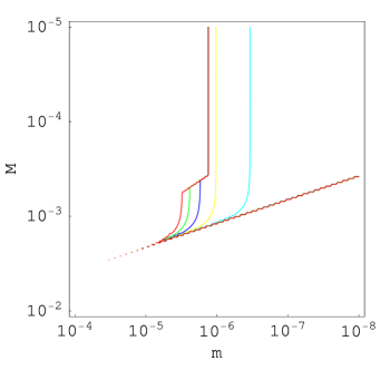
Figure 1: Contour plot of $n_{s}$ as a function of $m$ and $M$ for $0.9<n_{s}<1$, for the hybrid inflation model. The red, green, blue, yellow and light blue contours (from left to right) represent, respectively, $n_{s}$ equal to $0.91$, $0.93$, $0.95$, $0.97$ and $0.99$.

Analyzing the top plot in Fig. 2 we see that there is a small range of parameters for which $(n_{s},r)$ is inside the $68\%$ confidence level contour from WMAP only Kinney:2006qm . For this range we find

$$0.9525\lesssim n_{s}\lesssim 0.9975~{}~{}~{}~{}and~{}~{}~{}~{}0.05\lesssim r\lesssim 0.35.$$ (23)

For the range of parameters for which $(n_{s},r)$ is inside the $95\%$ confidence level contour we find

$$0.94\lesssim n_{s}\lesssim 1~{}~{}~{}~{}and~{}~{}~{}~{}0\lesssim r\lesssim 0.55.$$ (24)

Considering the results from WMAP + SDSS Kinney:2006qm we see that, looking to the bottom plot in Fig. 2, the range of parameters for which $(n_{s},r)$ is inside the $68\%$ confidence level contour is smaller than in the previous case. For this range we find

$$0.96\lesssim n_{s}\lesssim 0.995~{}~{}~{}~{}and~{}~{}~{}~{}0.05\lesssim r\lesssim 0.175.$$ (25)

For the range of parameters for which $(n_{s},r)$ is inside the $95\%$ confidence level contour we have

$$0.95\lesssim n_{s}\lesssim 1~{}~{}~{}~{}and~{}~{}~{}~{}0\lesssim r\lesssim 0.3.$$ (26)

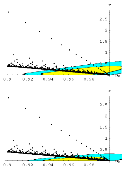
Figure 2: Plots of $r$ as a function of $n_{s}$ for $0.9<n_{s}<1$ (the black dots represent the different values of $M$ and $m$), for the hybrid inflation model, with the $68\%$ (yellow) and $95\%$ (blue) confidence level contours from WMAP (top) and WMAP + SDSS (bottom), taken from Kinney:2006qm .

Observing the plot in Figure 3 we see that the closer one gets to large values of $M$ the larger are the values of $r$ (i.e., the energy scale of inflation increases when $M$ increases) and $\alpha_{s}$. Analyzing the plot in Figure 4 we see that the closer one gets to small values of $\phi_{50}$ the larger are the values of $r$ (and so also the values of $\alpha_{s}$ get larger). We also note that $\phi_{50}$ is never much smaller than $1$, i.e., the Planck mass. Looking to the plot in Figure 5 we note that the energy density ratio is never much larger than $1$, which means that there is never a real false vacuum domination of the energy density, otherwise we would have $n_{s}\geq 1$. We also see that the closer one gets to the false vacuum domination cases (which occur for large values of $M$) the larger are the values of $r$ and the larger (and positive) are the values of the the running $\alpha_{50}$.

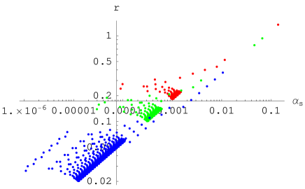
Figure 3: Plot of $r$ as a function of $\alpha_{s}$ for $0.945<n_{s}<0.955$ (red), $0.965<n_{s}<0.975$ (green) and $0.985<n_{s}<0.995$ (blue), for the hybrid inflation model.

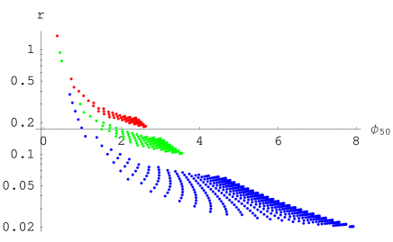
Figure 4: Plot of $r$ as a function of $\phi_{50}$ for $0.945<n_{s}<0.955$ (red), $0.965<n_{s}<0.975$ (green) and $0.985<n_{s}<0.995$ (blue), for the hybrid inflation model.

From this analysis we see that when we have false vacuum domination and small values of $\phi_{50}$, i.e., when we are more distant from chaotic inflation, then the values of the the running $\alpha_{50}$ are large and positive, which is in contradiction with the WMAP three-year results Kinney:2006qm . Also the values of the tensor-to-scalar ratio $r$ tend to be very large for these cases, which is also in disagreement with the observations.

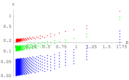
Figure 5: Plot of $r$ as a function of $E$ for $0.945<n_{s}<0.955$ (red), $0.965<n_{s}<0.975$ (green) and $0.985<n_{s}<0.995$ (blue), for the hybrid inflation model.

When $M$ goes to very small values we recover the results for chaotic inflation, which correspond to the lower limit for $r$ along the values of $n_{s}$ in Fig. 2. For these cases, for which $\phi_{50}$ is very large and the energy density ratio very small, we have small values for $\alpha_{50}$ and $r$, which is in very good agreement with the WMAP three-year results Kinney:2006qm .

III Conclusions

We have found that there is an intermediate regime for the original hybrid inflation model compatible with $n_{s}<1$, but as one approaches the false vacuum dominated limit within this regime the tensor-to-scalar ratio, $r$, and the running of the spectral tilt, $\alpha_{s}$, become large (with a positive running), which is in contradiction with the WMAP three-year results Kinney:2006qm . This agrees with the results in deVega:2006hb ; Peiris:2006ug ; Martin:2006rs . We found a lower bound on the allowed values of $r$, which might be an observational signal for hybrid inflation because if there is an upper bound on the spectral index, $n_{s}<1$, then we find a lower bound on the tensor-to-scalar ratio. This lower bound corresponds to chaotic inflation, which is in good agreement with the new WMAP results Kinney:2006qm . We also saw that it is difficult to get $\phi_{50}$ smaller than the Planck scale because decreasing $\phi_{50}$ requires us to increase the vacuum energy scale, $M$, and this increases the tensor-to-scalar ratio, $r$.

The inverted hybrid inflation model (see Appendix) is in much better agreement with the WMAP three-year results Kinney:2006qm than the original hybrid inflation model when we consider the false vacuum dominated regimes, especially because there is no lower bound on the allowed values of $r$. Moreover, in the inverted hybrid model there is no problem obtaining small values for $\phi_{50}\ll 1$, which makes these model easier to implement within supergravity Lyth:1998xn .

Appendix: The inverted hybrid inflation model

If we invert the sign of the inflaton energy density in Eq. (2) we get

$$V(\phi)=M^{4}-\frac{1}{2}m^{2}\phi^{2},$$ (27)

which corresponds to the potential for the inverted hybrid inflation model with a quadratic potential for the inflaton. A particular case of this model are the small-field inflation models Bassett:2005xm , for which the potential in Eq. (27) corresponds to a Taylor expansion about the origin and higher order terms are required to provide a potential minimum at some $\phi\neq 0$, as required to connect to a reheating stage (which is necessary to make the model realistic). So the inflaton starts with an initial small (positive) value and rolls down towards the minimum at a larger value, then it starts to oscillate and inflation ends with the end of slow-roll.

All the equations obtained before for the original hybrid inflation model, except Eq. (14), are still valid but with $m^{2}$ replaced by $-m^{2}$. To find the value of $\phi_{\epsilon}$ we search for the solutions of Eq. (12) with $\epsilon$ equal to $1$ (there are two different solutions for this equation but the results do not depend on which solution we choose).

.1 Results and discussion

In this case we have run the same code (with the appropriate changes in the equations) but for $m$ between $10^{-4}$ and $10^{-10}$ and $M$ between $10^{-2}$ and $10^{-6}$. The energy density ratio, Eq. (3), is evaluated $50$ e-folds after the inflaton has the value $\phi_{50}$.

Note that also in this case the selection of the values of $M$ is logarithmic, as one can see looking to the plot in Figure 6.

Figure 6: Contour plot of $n_{s}$ as a function of $m$ and $M$ for $0.9<n_{s}<1$, for the inverted hybrid inflation model. The red, green, blue, yellow and light blue contours (from left to right) represent, respectively, $n_{s}$ equal to $0.91$, $0.93$, $0.95$, $0.97$ and $0.99$.

Analyzing the top plot in Fig. 7 we see that there is a much wider range of parameters for which $(n_{s},r)$ is inside the $68\%$ confidence level contour from WMAP only Kinney:2006qm than in the original hybrid case, especially because there is no lower bound on the allowed values of $r$, in contrast with the original hybrid inflation model. For this range we find

$$0.935\lesssim n_{s}\lesssim 0.9875~{}~{}~{}~{}and~{}~{}~{}~{}0\lesssim r\lesssim 0.0775.$$ (28)

For the range of parameters for which $(n_{s},r)$ is inside the $95\%$ confidence level contour we get

$$0.9175\lesssim n_{s}\lesssim 1~{}~{}~{}~{}and~{}~{}~{}~{}0\lesssim r\lesssim 0.0775.$$ (29)

Observing the bottom plot in Fig. 7 we can see that there is also a wide range of parameters for which $(n_{s},r)$ is inside the $68\%$ confidence level contour from WMAP + SDSS Kinney:2006qm . For this range we get

$$0.935\lesssim n_{s}\lesssim 0.9925~{}~{}~{}~{}and~{}~{}~{}~{}0\lesssim r\lesssim 0.0775,$$ (30)

and for the range of parameters for which $(n_{s},r)$ is inside the $95\%$ confidence level contour we find

$$0.92\lesssim n_{s}\lesssim 1~{}~{}~{}~{}and~{}~{}~{}~{}0\lesssim r\lesssim 0.0775.$$ (31)

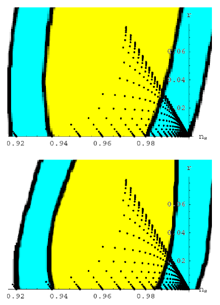
Figure 7: Plots of $r$ as a function of $n_{s}$ for $0.9<n_{s}<1$ (the black dots represent the different values of $M$ and $m$), for the inverted hybrid inflation model, with the $68\%$ (yellow) and $95\%$ (blue) confidence level contours from WMAP (top) and WMAP + SDSS (bottom), taken from Kinney:2006qm .

Looking to the plot in Figure 8 we see that the closer one gets to large values of $M$ the smaller are the values of $r$ and $\alpha_{s}$ (although we note that they are always small, even in the cases for which $M$ is small). Analyzing the plot in Figure 9 we see that the closer one gets to small values of $\phi_{50}$ the smaller are the values of $r$ (and so also the values of $\alpha_{s}$ get smaller). We note that here $\phi_{50}$ can be much smaller than the Planck mass. Observing the plot in Figure 10 we see that the closer one gets to the more false vacuum domination cases (which occur for large values of $M$) the smaller are the values of $r$ (and so also the values of $\alpha_{s}$). In this case we note that the energy density ratio can be very large, so we can have a strong vacuum domination.

Figure 8: Plot of $r$ as a function of $\alpha_{s}$ for $0.945<n_{s}<0.955$ (red), $0.965<n_{s}<0.975$ (green) and $0.985<n_{s}<0.995$ (blue), for the inverted hybrid inflation model.

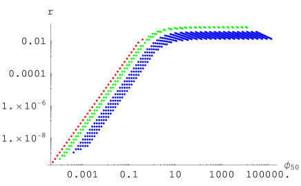
Figure 9: Plot of $r$ as a function of $\phi_{50}$ for $0.945<n_{s}<0.955$ (red), $0.965<n_{s}<0.975$ (green) and $0.985<n_{s}<0.995$ (blue), for the inverted hybrid inflation model.

From the previous analysis we see that for the inverted hybrid inflation model we can have, specially for large $M$, very small values for $r$ and $\alpha_{s}$, which is in very good agreement with the WMAP three-year results Kinney:2006qm . For these cases $\phi_{50}$ is also very small (it can be much smaller than $1$, i.e., the Planck mass) and $E$ is much larger than $1$, which means that there is a large false vacuum domination of the energy density. Therefore we can conclude that this model is in much better agreement with the WMAP results than the original hybrid inflation model when we consider the false vacuum domination regimes, especially because there is no lower bound on the allowed values of $r$. Moreover, in this model there is no problem obtaining small values for $\phi_{50}\ll 1$, which makes these model easier to implement within supergravity Lyth:1998xn .

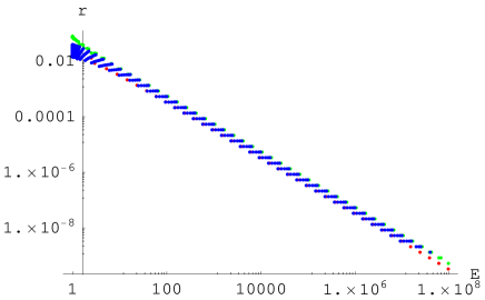
Figure 10: Plot of $r$ as a function of $E$ for $0.945<n_{s}<0.955$ (red), $0.965<n_{s}<0.975$ (green) and $0.985<n_{s}<0.995$ (blue), for the inverted hybrid inflation model.

References

• (1) D.ย N.ย Spergel et al., arXiv:astro-ph/0603449.
• (2) A.ย D.ย Linde, Phys.ย Rev.ย D 49 (1994) 748 [arXiv:astro-ph/9307002].
• (3) E.ย J.ย Copeland, A.ย R.ย Liddle, D.ย H.ย Lyth, E.ย D.ย Stewart and D.ย Wands, Phys.ย Rev.ย D 49 (1994) 6410 [arXiv:astro-ph/9401011].
• (4) D.ย H.ย Lyth and A.ย Riotto, Phys.ย Rept.ย  314 (1999) 1 [arXiv:hep-ph/9807278].
• (5) W.ย H.ย Kinney, E.ย W.ย Kolb, A.ย Melchiorri and A.ย Riotto, Phys.ย Rev.ย D 74 (2006) 023502 [arXiv:astro-ph/0605338].
• (6) H.ย Peiris and R.ย Easther, JCAP 0607 (2006) 002 [arXiv:astro-ph/0603587].
• (7) H.ย J.ย de Vega and N.ย G.ย Sanchez, arXiv:astro-ph/0604136.
• (8) J.ย Martin and C.ย Ringeval, JCAP 0608 (2006) 009 [arXiv:astro-ph/0605367].
• (9) D.ย H.ย Lyth and E.ย D.ย Stewart, Phys.ย Rev.ย D 54 (1996) 7186 [arXiv:hep-ph/9606412].
• (10) A.ย D.ย Linde, Phys.ย Lett.ย B 129 (1983) 177.
• (11) B.ย A.ย Bassett, S.ย Tsujikawa and D.ย Wands, arXiv:astro-ph/0507632.