Simulated X-ray galaxy clusters at the virial radius: slopes of the gas density, temperature and surface brightness profiles

Abstract

Using a set of hydrodynamical simulations of 9 galaxy clusters with masses in the range $1.5\times 10^{14}M_{\odot}<M_{\rm vir}<3.4\times 10^{15}M_{\odot}$, we have studied the density, temperature and X-ray surface brightness profiles of the intra-cluster medium in the regions around the virial radius. We have analyzed the profiles in the radial range well above the cluster core, the physics of which are still unclear and matter of tension between simulated and observed properties, and up to the virial radius and beyond, where present observations are unable to provide any constraints. We have modeled the radial profiles between $0.3R_{200}$ and $3R_{200}$ with power laws with one index, two indexes and a rolling index. The simulated temperature and [0.5–2] keV surface brightness profiles well reproduce the observed behaviours outside the core. The shape of all these profiles in the radial range considered depends mainly on the activity of the gravitational collapse, with no significant difference among models including extra-physics. The profiles steepen in the outskirts, with the slope of the power-law fit that changes from -2.5 to -3.4 in the gas density, from -0.5 to -1.8 in the gas temperature, and from -3.5 to -5.0 in the X-ray soft surface brightness. We predict that the gas density, temperature and [0.5–2] keV surface brightness values at $R_{200}$ are, on average, $0.05$, $0.60$, $0.008$ times the measured values at $0.3R_{200}$. At $2R_{200}$, these values decrease by an order of magnitude in the gas density and surface brightness, by a factor of 2 in the temperature, putting stringent limits on the detectable properties of the intracluster-medium (ICM) in the virial regions.

1 Introduction

Galaxy clusters form in correspondence of the highest peaks of the fluctuations in the cosmic dark matter density field and collapse under the action of gravitational attraction to define structures with a mean density enhanced with respect to the cosmic value by a factor of few hundreds. They reach the virial equilibrium over a volume with a typical virial radius that indicates, as a first approximation, the regions where the pristine gas accretes on the dark matter halo through gravitational collapse and is heated up to millions degrees through adiabatic compression and shocks. This intracluster-medium (ICM), that represents about 80 (15) per cent of the baryonic (total) cluster mass (e.g. Ettori et al., 2004), becomes, then, X-ray emitter mainly through bremsstrahlung processes, thus allowing one to trace and characterize the distribution of the baryonic and dark matter components.

From an observational point of view, the measurement of the properties of the ICM is possible only where the X-ray emission can be well resolved against the background (both instrumental and cosmic). At the present, data permit to firmly characterize observables like surface brightness (see Mohr et al., 1999; Ettori & Fabian, 1999) and gas temperature (see Markevitch et al., 1998; De Grandi & Molendi, 2002; Pointecouteau et al., 2005; Vikhlinin et al., 2006; Zhang et al., 2006) out to a fraction ($\sim 0.5-0.6$) of the virial radius. Only few examples of nearby X-ray bright clusters with surface brightness estimated out to the virial radius are available, thanks to the good spatial resolution, the large field-of-view and the low instrumental background of the ROSAT/PSPC instrument (Vikhlinin et al., 1999; Neumann, 2005). However, since the regions not-yet resolved occupy almost 80 per cent of the total volume, they retain most of the information on the processes that characterize the accretion and evolution within the cluster of the main baryonic component (Molendi, 2004).

Table 1: List of main physical parameters of the 9 clusters taken from the ovisc runs. The objects are divided into 2 subsamples according to their virial mass. Note that $T_{\rm vir}$ is the average mass-weighted temperature of the gas up to $R_{\rm vir}$ while $T_{200}$ is the temperature of the gas at $R_{200}$.

	Sample $A$: $M_{\rm vir}>10^{15}M_{\odot}$						Sample $B$: $M_{\rm vir}<10^{15}M_{\odot}$
Cluster name	g1	g8	g51	g72			g676	g914	g1542	g3344	g6212
$M_{\rm vir}$ ($10^{15}M_{\odot}$)	2.12	3.39	1.90	1.96			0.15	0.17	0.15	0.16	0.16
$R_{\rm vir}$ (Mpc)	3.37	3.94	3.25	3.28			1.40	1.46	1.40	1.43	1.43
$T_{\rm vir}$ (keV)	6.49	9.89	5.78	5.44			1.25	1.28	1.18	1.26	1.22
$R_{200}$ (Mpc)	2.48	2.91	2.39	2.40			1.04	1.08	1.04	1.05	1.05
$T_{200}$ (keV)	4.18	7.52	4.18	4.09			0.82	1.03	0.83	0.88	0.84

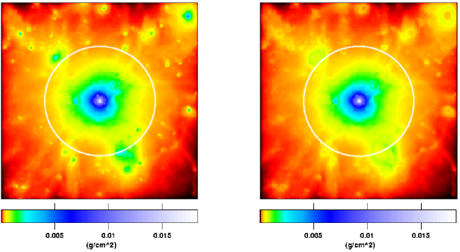
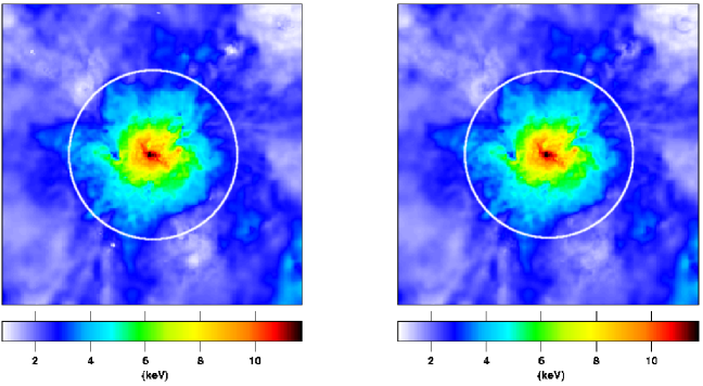
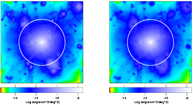
Figure 1: From top to bottom: maps of the projected gas density, mass-weighted temperature and soft (0.5-2 keV) X-ray emission of the g1 cluster (csf model) for the 100 per cent (left) and 95 per cent (right) volume-selection scheme. The circles indicate the virial radius. The size of the side of each map is 12 Mpc, so they cover roughly up to $2.5R_{200}$.

In the present work, we study the distribution of the ICM density, temperature and surface brightness in a set of simulated galaxy clusters by looking at their radial profiles in the range between $0.3-3\times R_{200}$. We avoid considering the regions where the clusters evolve a core with active cooling and suspected feedback regulation, being this balance still matter of tension between the present simulated constraints and the observed counterparts (e.g. Borgani et al., 2004). Therefore, we concentrate our analysis on cluster volumes where the gas density and temperature suggest that radiative processes are not dominant and the main physical driver is just the gravitational collapse, that is expected to be well described in the present numerical N-body simulations. We consider objects extracted from a dark matter only cosmological simulation that were resimulated at much higher resolution by including the gas subjected to gravitational heating and other physical treatments like cooling, star formation, feedback, thermal conduction and an alternative implementation of artificial viscosity.

We organize this paper in the following way: in the next Section, we describe our dataset of simulated clusters and their different physical properties; in Section 3 we discuss the results on the slopes of the gas temperature, density and surface brightness profiles in the outskirts (i.e. $r>0.3R_{200}$) of the simulated objects and compare our results with the present constraints obtained from X-ray observations of bright clusters. We summarize and discuss our results in Section 4.

2 The simulated clusters

For the purpose of this work we use a set of 9 resimulated galaxy clusters extracted from a dark matter (DM)-only simulation of a “concordance” $\Lambda$CDM model with $\Omega_{\rm m}=0.3$ and $\Omega_{\Lambda}=0.7$, using a Hubble parameter $h=0.7$ (the Hubble constant being $H_{0}=h\ 100$ km s^-1Mpc^-1) and a baryon fraction of $\Omega_{\rm b}=0.019h^{-2}$. The initial conditions of the parent simulation, that followed the evolution of a comoving box of $479h^{-1}$ Mpc per size, were set considering a cold dark matter power spectrum normalized by assuming $\sigma_{8}=0.9$ (see Yoshida et al., 2001). Our simulations were carried out using GADGET-2 (Springel, 2005), a new version of the Tree-Smoothing Particles Hydrodynamics (SPH) parallel code GADGET (Springel et al., 2001) which includes an entropy-conserving formulation of SPH (Springel & Hernquist, 2002) and a treatment of many physical processes affecting the baryon component that can be turned on and off to study their influence on the thermodynamics of the gas. In the volume of the parent simulation 9 different haloes were identified, spanning different mass ranges: 4 of them with the typical dimension of clusters and 5 of small clusters or group-like objects. Then using the ”Zoomed Initial Conditions” (ZIC) technique (Tormen et al., 1997) they were resimulated by identifying their corresponding Lagrangian regions in the initial domain and populating them with more particles (of both DM and gas), while appropriately adding high-frequency modes. At the same time the volume outside the region of interest was resimulated using low-resolution (LR) particles in order to follow the tidal effects of the cosmological environment. The setup of initial conditions of all the resimulations was optimized to guarantee a volume around the clusters of $\sim 5R_{\rm vir}$ free of contamination from LR particles. This was obtained using an iterative process as follows. Starting from a first guess of the high-resolution (HR) region that we want to resimulate, we run a DM-only re-simulation. Analyzing its final output, we identify all the particles that are at distances smaller than 5 $R_{\rm vir}$ from the cluster centre in order to identify the corresponding Lagrangian region in the initial domain. Applying ZIC, we generate new initial conditions at higher resolution and run one more DM-only resimulation. This procedure is iteratively repeated until we find that none of the LR particles enters the HR region, which could be possible because of the introduction of low-scale modes. Thus we can safely say that these resimulations are representing the external regions of our cluster without any spurious numerical effect.

These resimulations are set to have a mass resolution of $m_{\rm DM}=1.13\times 10^{9}h^{-1}M_{\odot}$ for DM particles and $m_{\rm gas}=1.69\times 10^{8}h^{-1}M_{\odot}$ for baryons, so that every resimulated cluster is resolved with between $2\times 10^{5}$ and $4\times 10^{6}$ particles (both DM and gas) depending on its final mass. All the simulations have a (Plummer-equivalent) softening-length kept fixed at $\varepsilon=30h^{-1}$ kpc comoving at $z>5$ and switched to a physical softening length $\epsilon=5h^{-1}$ kpc at lower redshifts.

In order to study the impact of different physical processes on the clusters properties, we simulated every cluster using 4 different sets of physical models:

1. Gravitational heating only with an ordinary treatment of gas viscosity (which will be referred as the ovisc model).

2. Gravitational heating only but with an alternative implementation of artificial viscosity (lvisc model), following the scheme proposed by Morris & Monaghan (1997), in which every gas particle evolves with its own viscosity parameter. With this implementation the shocks produced by gas accretion are as well captured as in the ovisc model, while regions with no shocks are not characterized by a large residual numerical viscosity. As already studied in Dolag et al. (2005), this scheme allows to better resolve the turbulence driven by fluid instabilities, thus allowing clusters to build up a sufficient level of turbulence-powered instabilities along the surfaces of the large-scale velocity structures present in cosmic structure formation.

3. Runs which implement a treatment of cooling, star formation and feedback (csf model). The star formation is followed by adopting a sub-resolution multiphase model for the interstellar medium which includes also the feedback from supernovae (SN) and galactic outflows (Springel & Hernquist, 2003). The efficiency of SN to power galactic winds has been set to 50 per cent, which turns into a wind speed of 340 km/s.

4. Runs like csf but also including thermal conduction (csfc model), adopting the scheme described by Jubelgas et al. (2004). This implementation in SPH, which has been proved to be stable and to conserve the thermal energy even when individual and adaptive time-steps are used, assumes an isotropic effective conductivity parametrized as a fixed fraction of the Spitzer rate (1/3 in our simulations). It also accounts for saturation which can become relevant in low-density regions. For more details on the properties of simulated clusters using this model, see also Dolag et al. (2004).

The masses, radii and temperatures of the 9 clusters for the ovisc model are summarized in Table LABEL:tab:9clusters. The other models have similar results for masses and radii with variation of few percent between the models while temperatures have larger variations with csf and csfc models having slightly higher temperatures ($\sim 8$ per cent). In our following analyses we will separate the clusters into two different samples: sample $A$ (4 clusters) and $B$ (5) according to their virial mass being larger or smaller than $10^{15}M_{\odot}$, respectively.

When considering the environmental properties of these haloes, we must point out that the 4 objects of sample $A$ are among the most massive clusters of the volume of the parent simulation while the 5 groups were chosen at random with the only condition to be far away from the 4 clusters. At the end of the resimulations all the haloes of sample $B$ appear to be isolated, e.g. there is no halo with mass $M>10^{13.5}h^{-1}M_{\odot}$ at distance lower than $5R_{\rm vir}$; on the contrary the big clusters have several small structures inside the volume of their resimulation and all of them underwent significant merging activities. As we will see in Section 3, this aspect is important to understand the different properties of the X-ray profiles of the two samples.

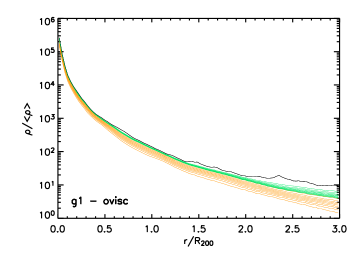
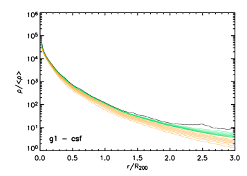
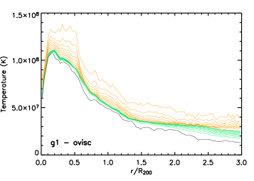
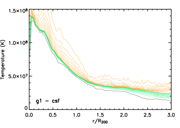
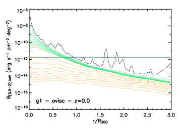
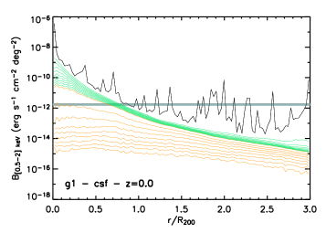
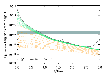
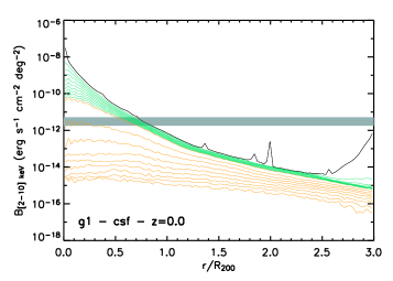
Figure 2: Radial profiles for different quantities as estimated for the g1 cluster. From top to bottom: gas density (normalized to the cosmic mean density, $<\rho>\equiv\Omega_{\rm b}\rho_{\rm c}$), mass-weighted temperature and X-ray surface brightness for the soft (0.5–2 keV) and the hard (2–10 keV) band calculated considering the clusters at $z=0$. Left column: ovisc model. Right column: csf model. These profiles are obtained from different prescriptions: the black line shows the average of all the gas particles, the orange lines are averages of the different volume percentages from 10 to 90 per cent and the green lines are from 91 to 99 per cent. The extragalactic unresolved background from Hickox & Markevitch (2006) in the [0.5–2] keV and [2–8] keV band of is indicated by the shaded region in the soft and hard X-ray surface brightness panels, respectively.

2.1 Preparation of the dataset

Focusing our attention on the cluster outskirts, we do not consider in our study the effects of the cluster core on the overall properties, avoiding to deal with the theoretical, numerical and observational uncertainties on the physics of the X-ray emitting plasma in the cluster central regions. Furthermore we must take into account that the mass enclosed in a given radial bin in the external regions of clusters ($r>R_{200}$) is dominated by the presence of dense subclumps of the typical dimension of galaxies or small galaxy-groups ($M\la 10^{13}M_{\odot}$). Evidences of the existence of these clumps in the regions inside $R_{200}$ have also been shown by X-ray observations, but it is still not clear whether the frequency and the emission properties of the simulated clumps agree with the observed ones: this is due both to the low surface brightness of these objects that makes them difficult to resolve and to uncertainties in the theoretical modeling (e.g. simulations including cooling tend to produce more clumps and simulations with feedback from SNe end up with smaller clumps than non-radiative ones).

Anyway, since (i) we are interested only in the average properties of galaxy clusters and (ii) these small clumps are generally masked out in observational works, a direct comparison of our simulations with theoretical and observational results requires the introduction of a method to exclude these cold and dense clumps from our analysis. It is quite difficult to define a precise and unique criterium to identify these condensed regions in the simulation volume from their dynamical and thermodynamical properties, therefore we decided to identify the volumes corresponding to non-collapsed regions. For this purpose we proceed in the following way: for every shell that corresponds to a radial bin of the profile, we sort the gas particles in decreasing volume order (i.e. starting from the more diffuse particles and going up to the denser ones, being the volume associated to the $i$-th particle defined as $V_{i}=m_{\rm gas}/\rho_{{\rm gas,}i}$) then we compute the profiles calculating the mean of a given quantity considering only the particles summing up to a given percentage of the total volume of the shell. In order to identify the physical properties of the regions excluded by our analysis, we plot in Fig. 1 as an example the maps of the projected density, mass-weighted temperature and soft (0.5-2 keV) X-ray surface brightness of the g1 cluster considering (i) all the particles and (ii) those that are within the 95 per cent volume of each radial shell. We can clearly see from these maps that the volume-selective method actually separates the cold and dense clumps from the rest of the object. Anyway these maps show that this criterion is much more effective in excluding dense regions than cold ones. However, since the X-ray emission is strongly dependent on the density of the gas, we can safely say that it well mimics the observational technique of masking the bright isolated regions.

We also study the shapes of X-ray surface brightness profiles of our simulated clusters. Since we are interested in the outskirts of galaxy clusters we cannot adopt a pure bremsstrahlung emission model because in the corresponding temperature ranges ($T<$ 1 keV) line emission gives a significant contribution. Therefore in order to calculate the profiles we adopt a MEKAL emission model (Mewe et al., 1985; Liedahl et al., 1995) assuming a gas metallicity $Z=0.2Z_{\odot}$ (using the solar value tabulated in Anders & Grevesse, 1989) constant for every particle of the simulation: although this value can be an underestimate of the metallicity of the clusters’ centre (see De Grandi et al., 2004, for more detail), the chosen model can be considered a good representation of the spectral properties of the clusters’ external regions. In the following analyses we consider the objects at redshift $z=0$. To compute the surface brightness profiles, we adopted the same volume-selection scheme of the density and temperature profiles with the only difference that, since we want to obtain the surface brightness profiles of our objects, we need to take into account the two-dimensional projection on the sky plane. To this purpose, we consider circular ring sections instead of spherical shells: for every ring, we select all the particles that fill a given volume fraction $f$, we calculate their luminosity and we obtain $L_{f}$ by summing all of them. Finally we normalize it to take into account also for the remaining volume and use the normalized luminosity $L_{ring}=\frac{L_{f}}{f}$ to calculate the surface brightness (see the effects of this method on the [0.5-2] keV X-ray surface brightness shown in the bottom panel of Fig. 1). This method works efficiently for subtracting almost all the relevant substructures in the surface brightness profiles, except for two massive subhaloes present in the g1 cluster simulation at a distance of 2-3 $R_{200}$ from the center; only for this cluster we excluded two separate angular regions (45 degrees wide each) from the computation of its X-ray surface brightness profiles.

In Fig. 2, we show the gas density, temperature and surface brightness profiles into two different bands for a massive cluster (g1) assuming two different physical models: the “ordinary-viscosity non-radiative” (ovisc) and the “cooling + star formation + feedback” (csf) one. We plot the average profiles together with the ones obtained with different cuts in volume. The profiles in Fig. 2 show that eliminating the fraction of mass concentrated in 1 per cent of the volume is sufficient to make the gas density, temperature and surface brightness profiles much more regular than the average ones that consider all the particles in the shell. For these reasons in the following analyses, we will mainly concentrate in fitting the 99 per cent–volume profiles and discuss the results obtained by cutting the volume at different percentages in Appendix A. By the way we also note that the temperature and density profiles obtained with this method for the ovisc model well reproduce the shape of the theoretical profiles obtained by Ascasibar et al. (2006), if we assume a polytropic index $\gamma\simeq 1.18-1.20$.

In Fig. 3 we compare the 99 per cent volume profiles for one of the largest and the smallest cluster of the samples using the four different physical models. As already noted in Borgani et al. (2004), radiative cooling and star formation selectively remove low-entropy gas from high-density regions. Consequently models with cooling tend to produce clusters less dense at the centre ($r<0.1R_{200}$): in these regions we find that the gas density in non-radiative models is higher by a factor of $\sim 3.5$ in the most massive clusters and more than 5 in less massive ones. The same cooling processes generate a lack of pressure near the centre of the clusters that heats the infalling gas up to a factor of $\sim 1.8$ higher than in non-radiative simulations for all mass scales (see also Tornatore et al., 2003). As a result, the X-ray emission in the internal regions is significantly reduced in the csf and csfc models. The external regions of the clusters are less affected by the different physics because the low-density gas is less prone to cooling and feedback effects. As we will show later, this makes the results on the external regions of clusters only slightly dependent on the physical model adopted in the simulation (see also Romeo et al., 2006, for influences of other physical processes).

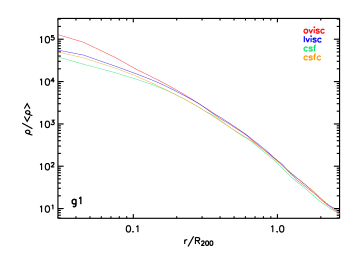
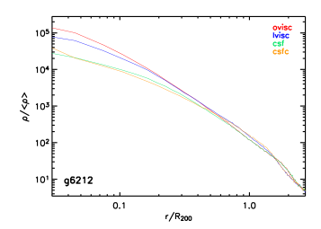
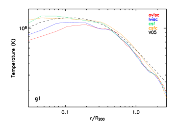
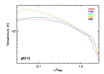
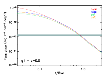
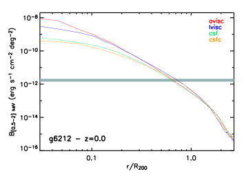
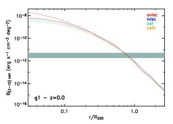
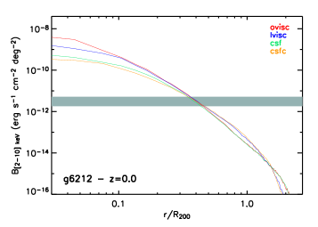
Figure 3: From top to bottom: comparison between the gas density (normalized to the cosmic mean density, $<\rho>\equiv\Omega_{\rm b}\rho_{\rm c}$), mass-weighted temperature, soft and hard X-ray surface brightness profiles extracted from the 99 per cent volume of the clusters g1 (left column) and g6212 (right column) simulated by using 4 different physical models. A dashed line indicates the functional form from Vikhlinin et al. (2006, eq. 9) that well reproduces the behaviour of the temperature profile of nearby bright galaxy clusters observed with Chandra. The functional form is normalized to the average values of the temperature obtained from the 4 models at $0.5R_{200}$. The extragalactic unresolved background from Hickox & Markevitch (2006) in the [0.5–2] keV and [2–8] keV band of is indicated by the shaded region in the soft and hard X-ray surface brightness panels, respectively.

In Fig. 4 we compare the 99 per cent volume profiles for the 4 most massive clusters of the dataset (sample $A$). The density profiles have a very similar shape up to about $2R_{200}$ indicating a universal function. The regularity of the 99 per cent volume profiles extends also for distances $>3R_{200}$. The temperature profiles are more irregular (note that the temperatures are normalized using $T_{200}$, the temperature at $R_{200}$ ): the bumps present in the g1 profile near the centre and in g72 at $r\sim 1.7R_{200}$ are an effect of shocks at $r\sim 0.6R_{200}$ and $r\sim 2.1R_{200}$, respectively, due to recent major mergers.

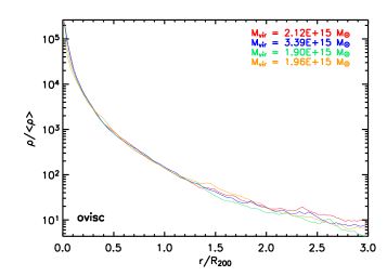
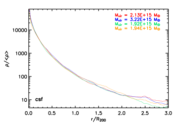
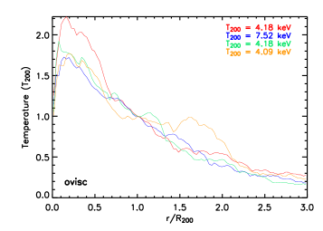
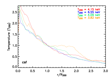
Figure 4: Comparison between the 99 per cent volume profiles of density (normalized to the cosmic mean density, $<\rho>\equiv\Omega_{\rm b}\rho_{\rm c}$) (top panels) and mass-weighted temperature normalized to $T_{200}$ (lower panels) for the clusters g1 (red), g8 (blue), g51 (green), g72 (orange). Left and right columns refer to the ovisc and csf model, respectively.

In Table 2 we show the ratios between the values of the 99 per cent volume profiles at different radial distances and their values at $0.3R_{\rm vir}$ obtained with the ovisc model. The regularity of these profiles can be seen by the low dispersion between the values of the clusters of the same sample.

Table 2: Ratios between the profile values at different radial distances and their values at $0.3R_{200}$. We show the average and the standard deviation between the two cluster samples for the ovisc model.

Radial distance ($R_{200}$)	0.3	0.5	0.7	1.0	2.0	3.0
	Sample $A$
$\rho$	$1.0$	$0.31\pm 0.02$	$0.127\pm 0.004$	$(4.8\pm 0.2)\times 10^{-2}$	$(5.6\pm 0.8)\times 10^{-3}$	$(1.7\pm 0.5)\times 10^{-3}$
$T$	$1.0$	$0.88\pm 0.06$	$0.72\pm 0.06$	$0.60\pm 0.06$	$0.34\pm 0.09$	$0.16\pm 0.03$
$SB_{[0.5-2]{\rm keV}}$	$1.0$	$0.17\pm 0.03$	$(4.0\pm 1.1)\times 10^{-2}$	$(8.4\pm 1.2)\times 10^{-3}$	$(2.3\pm 0.9)\times 10^{-4}$	$(6.3\pm 4.3)\times 10^{-5}$
$SB_{[2-10]{\rm keV}}$	$1.0$	$0.15\pm 0.02$	$(3.2\pm 0.1)\times 10^{-2}$	$(5.5\pm 0.1)\times 10^{-3}$	$(7.1\pm 1.8)\times 10^{-5}$	$(6.4\pm 5.7)\times 10^{-6}$
	Sample $B$
$\rho$	$1.0$	$0.31\pm 0.02$	$0.13\pm 0.02$	$(4.8\pm 0.7)\times 10^{-2}$	$(6.0\pm 0.2)\times 10^{-3}$	$(1.6\pm 0.2)\times 10^{-3}$
$T$	$1.0$	$0.84\pm 0.04$	$0.72\pm 0.04$	$0.58\pm 0.03$	$0.29\pm 0.06$	$0.14\pm 0.02$
$SB_{[0.5-2]{\rm keV}}$	$1.0$	$0.16\pm 0.02$	$(4.2\pm 1.1)\times 10^{-2}$	$(7.9\pm 1.0)\times 10^{-3}$	$(1.8\pm 0.9)\times 10^{-4}$	$(1.5\pm 1.0)\times 10^{-5}$
$SB_{[2-10]{\rm keV}}$	$1.0$	$0.11\pm 0.01$	$(2.1\pm 0.7)\times 10^{-2}$	$(2.3\pm 0.4)\times 10^{-3}$	$(1.7\pm 1.4)\times 10^{-5}$	$(5.6\pm 7.2)\times 10^{-7}$

3 Results on the outer slopes of the radial profiles

To describe the behaviour of the radial density and temperature profiles in the cluster outskirts, we adopt a broken power-law relation given by the expression

$$y(x)=\left\{\begin{array}[]{ll}ax^{-b_{1}}&\mbox{if $x\leq R_{b}/R_{200}$}\\ a\left(\frac{R_{b}}{R_{200}}\right)^{-(b_{1}-b_{2})}x^{-b_{2}}&\mbox{if $x>R_{b}/R_{200}$}\end{array}\right.\ ,$$ (1)

in its logarithmic form, where $r$ is the distance from the centre, $x\equiv r/R_{200}$ and $a$, $b_{1}$, $b_{2}$ and $R_{b}$ are the free parameters, representing the normalization, the inner slope, the outer slope and the radius at which the slope changes, respectively. The fit is computed in the interval $0.3\leq x\leq 2.7$. We fit the profiles for the 9 clusters separately and then calculate the average and dispersion for every parameter. The best fit relations for the ovisc model are shown together with the profiles of single clusters in Fig. 5.

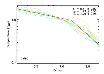
Figure 5: Profiles (99 per cent volume) of the 9 clusters obtained with the ovisc model. The orange lines are for the 4 clusters of sample $A$, the green lines are for the 5 groups of sample $B$. We fit the data with a broken power-law relation of eq. 1 in the interval $0.3\leq r/R_{\rm 200}\leq 2.7$ and plot (black line) the relation assuming the average of the best-fit parameters between the 9 objects.

The gas density profiles show a change in the slope of the power law at about 1.1-1.3 $R_{200}$, with an internal slope of 2.4-2.5 with no significant dependence on the physical model or the volume selection scheme adopted (see the Appendix for details on the effect of different volume cuts) and also a very low dispersion between the different objects. This indicates that the behaviour of the density profiles is well determined from outside the core to more than $R_{200}$. In the outskirts the slope increases up to $b_{2}\sim 3.4$ for all the models showing more dispersion between the 9 haloes due to the fact that in these regions the influence of the environment is becoming more important with respect to the potential well of the cluster itself.

In the temperature profiles, the steepening towards the external regions is more prominent and the cutoff is around $r=1.3-1.5R_{200}$ with significant dispersion between the clusters. The best fit internal slope is significantly affected by the physics: the profiles obtained with non-radiative simulations have slopes of $b_{1}\sim 0.4$ while csf and csfc models produce steeper profiles with slopes of $b_{1}\sim 0.6$. Also in the outskirts the non-radiative models tend to produce slightly shallower profiles with the difference less significant due to the higher dispersion between the different haloes. The different slopes of the profiles is an effect of the cooling that creates an higher gradient of temperature as can be seen in Fig. 3.

In Fig. 2, we also show the soft (0.5–2 keV) and hard (2–10 keV) X-ray surface brightness profiles of the g1 object for the different physical models. These plots indicate that models with cooling produce a higher number of clumps that dominate the soft X-ray emission in the external regions. These clumps are indeed those that are well eliminated by our selection in volume. We also obtain that the cluster surface brightness at $z=0$ reaches the value of the unresolved X-ray background estimated by Hickox & Markevitch (2006) of $1.76\pm 0.32$ in the [0.5–2] keV band and $3.5\pm 1.7$ in the [2–8] keV band in units of $10^{-12}$ erg s^-1 cm^-2 deg^-2, at approximately $0.8R_{200}$ and $0.4R_{200}$ in the soft and hard band, respectively; considering the effect of redshift dimming and that, according to the recent results of Roncarelli et al. (2006), a significant fraction of this background can be due to the diffuse gas of non-virialized objects, the perspective of observing the regions around the clusters virial radius is extremely challenging.

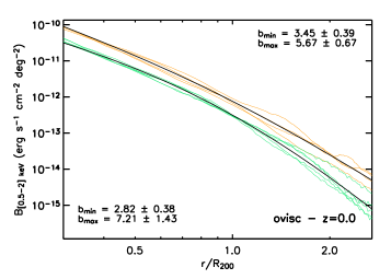
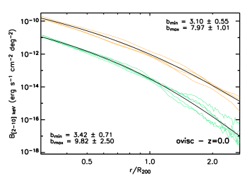
Figure 6: X-ray surface brightness profiles (99 per cent volume, [0.5–2] and [2–10] keV band) of the 9 clusters for the ovisc model. The orange lines are for the 4 clusters of sample $A$, the green lines are for the 5 groups of sample $B$. We fit the data of the two samples separately with a rolling-index power-law relation of eq. 2 in the interval $0.3\leq r/R_{\rm 200}\leq 2.7$ and plot (black lines) the relations assuming the average of the best-fit parameters between the objects of the samples.

Table 3: Distribution of the best-fit values of the rolling-index power-law functions (see eq. 2) of the soft (0.5–2 keV) and hard (2–10 keV) X-ray surface brightness profiles separated between the two samples $A$ and $B$ and for different physical models. The profiles are extracted from the 99 per cent volume-selection scheme and fitted over the radial range $0.3\leq r/R_{\rm 200}\leq 2.7$.

	Soft X-ray band
	[0.5–2] keV
	Sample $A$			Sample $B$
	$b_{\rm min}$	$b_{\rm max}$		$b_{\rm min}$	$b_{\rm max}$
ovisc	$3.45\pm 0.39$	$5.67\pm 0.67$		$2.82\pm 0.38$	$7.21\pm 1.43$
lvisc	$3.36\pm 0.33$	$5.73\pm 0.80$		$2.73\pm 0.79$	$7.72\pm 1.93$
csf	$3.49\pm 0.21$	$5.33\pm 0.57$		$2.50\pm 0.28$	$7.14\pm 1.14$
csfc	$2.76\pm 0.28$	$6.36\pm 1.09$		$1.99\pm 0.50$	$7.80\pm 1.76$
	Hard X-ray band
	[2–10] keV
	Sample $A$			Sample $B$
	$b_{\rm min}$	$b_{\rm max}$		$b_{\rm min}$	$b_{\rm max}$
ovisc	$3.10\pm 0.55$	$7.97\pm 1.01$		$3.42\pm 0.71$	$9.82\pm 2.50$
lvisc	$3.08\pm 0.29$	$7.87\pm 0.90$		$3.36\pm 1.72$	$10.48\pm 5.26$
csf	$3.25\pm 0.41$	$7.56\pm 0.73$		$3.25\pm 0.43$	$9.69\pm 2.66$
csfc	$1.94\pm 0.36$	$9.31\pm 2.11$		$2.87\pm 1.71$	$10.95\pm 5.79$

Since we observe a steepening of the slope of the X-ray profiles going to the external regions, we fit them with a rolling-index power law function

$$y=ax^{-b_{\rm max}\frac{x+b_{\rm min}/b_{\rm max}}{x+1}}\ ,$$ (2)

where $x\equiv r/R_{200}$, and $a$, $b_{\rm min}$ and $b_{\rm max}$ are the free parameters, with $b_{\rm min}$ and $b_{\rm max}$ representing the slope in the two asymptotic cases, $x\rightarrow 0$ and $x\gg 1$, respectively. We fit the two samples separately in the interval $0.3\leq r/R_{\rm 200}\leq 2.7$. The results for the 4 physical models are quoted in Tab. 3. The average best-fit values on the slopes of the surface brightness of the objects simulated with the ovisc model are shown in Fig. 6. Overall, the fits well reproduce the shape of the surface brightness in the interval $0.3\leq r/R_{200}\leq 2.7$. Our sample of galaxy “groups” (sample $B$) presents a soft X-ray profile that is (i) shallower in the centre ($b_{\rm min,B}\sim 2.7$, $b_{\rm min,A}\sim 3.4$) and (ii) steeper in the outskirts ($b_{\rm max,B}\sim 7.3$, $b_{\rm max,A}\sim 5.5$) than the one estimated in the sample of massive clusters (sample $A$). The following reasons can be considered to explain this behaviour: (i) the ICM temperature of the objects in sample $B$ at $R_{200}$ is below 1 keV (see Table LABEL:tab:9clusters) and decreases at $r>R_{200}$ to values that becomes comparable to (and less than) the lower end of the [0.5–2] keV band here considered, resulting in a cut-off of the soft X-ray signal. This also explains the steeper slope of the hard X-ray profiles in the less massive objects; (ii) the higher cooling efficiency in groups, with respect to rich clusters, enhances the selective removal of low-entropy gas from the hot phase, thus producing shallower profiles of X-ray emitting gas; (iii) as discussed at the end of Section 2, while our clusters are the most massive objects in the volume of the parent simulation and are still accreting material, the “groups” appear to be isolated, thus with less evidence of recent accretion activity. This results in slightly shallower profiles near the centre.

3.1 Comparison with observational constraints

Table 4: Distribution of the best-fit values of the power-law slopes of the X-ray surface brightness profiles separated between the two samples $A$ and $B$ ($b_{A}$ and $b_{B}$, respectively), the two X-ray bands and different physical models. The profiles extracted from the 99 per cent volume-selection scheme and fitted over the different radial ranges $x_{\rm min}-x_{\rm max}$ (in units of $R_{200}$.) Values of $b_{\rm obs}$ are the observational constraints in the same radial range from Neumann (2005) (see text in Section 3.1).

		Soft X-ray band				Hard X-ray band
		[0.5–2] keV				[2–10] keV
	$x_{\rm min}-x_{\rm max}$	$b_{A}$	$b_{B}$	$b_{\rm obs}$		$b_{A}$	$b_{B}$
ovisc	0.3 – 1.2	4.05$\pm$0.03	4.09$\pm$0.01	3.79$\pm$0.38		4.46$\pm$0.05	5.23$\pm$0.03
lvisc	0.3 – 1.2	4.04$\pm$0.04	4.14$\pm$0.09			4.47$\pm$0.05	5.32$\pm$0.17
csf	0.3 – 1.2	3.99$\pm$0.00	3.81$\pm$0.02			4.50$\pm$0.02	5.07$\pm$0.04
csfc	0.3 – 1.2	3.79$\pm$0.02	3.57$\pm$0.04			4.19$\pm$0.03	5.03$\pm$0.12
ovisc	0.7 – 1.2	4.49$\pm$0.19	4.76$\pm$0.32	5.73${}^{+1.43}_{-1.26}$		5.15$\pm$0.41	6.42$\pm$0.76
lvisc	0.7 – 1.2	4.54$\pm$0.32	4.66$\pm$0.19			5.26$\pm$0.44	6.20$\pm$0.75
csf	0.7 – 1.2	4.31$\pm$0.28	4.45$\pm$0.11			5.18$\pm$0.37	5.92$\pm$0.13
csfc	0.7 – 1.2	4.29$\pm$0.17	4.35$\pm$0.14			4.89$\pm$0.24	6.42$\pm$0.61
ovisc	1.2 – 2.7	5.15$\pm$0.62	6.37$\pm$0.93			6.95$\pm$0.88	8.43$\pm$1.70
lvisc	1.2 – 2.7	5.21$\pm$0.59	6.77$\pm$0.95			6.88$\pm$0.54	9.01$\pm$2.72
csf	1.2 – 2.7	4.90$\pm$0.53	6.23$\pm$0.67			6.70$\pm$0.74	8.40$\pm$1.52
csfc	1.2 – 2.7	5.67$\pm$0.63	6.58$\pm$0.88			8.14$\pm$1.32	9.14$\pm$3.36

Our results on the external shape of the gas density, temperature and surface brightness profiles in simulated galaxy clusters can be compared with recent estimates obtained for nearby X-ray bright objects. Neumann (2005) discusses the outer slope of the soft X-ray surface brightness in 14 clusters observed with ROSAT/PSPC. In order to compare our results with the ones of that work, we fit the 99 per cent volume X-ray profiles in different intervals for the two clusters samples with a single power-law function, $S(x)=a\,x^{-b}$, where $a$ and $b$ are the two free parameters and $x\equiv r/R_{200}$. We avoid to consider the interval $0.1\leq x\leq 0.3$, owing to the fact that this region is very model-dependent and cannot be represented by a single power-law relation. Our results are listed in Table 4 together with the corresponding results ($b_{\rm obs}$) of Neumann (2005). In the interval $0.3\leq x\leq 1.2$, for the sample of clusters labeled ”4” that better matches the virial temperatures of our sample $A$, Neumann (2005) measures a slope of $3.79\pm 0.38$ in good agreement with our average values of $(3.78,4.03)$, being the lower values measured in objects simulated with the inclusion of extra-physics (models csf and csfc). In the interval $0.7\leq x\leq 1.2$, the observational constraints are looser and are between $5.73^{+1.43}_{-1.26}$ for the 7 most massive clusters in the Neumann’s sample and $7.22^{+1.79}_{-1.60}$ for the whole dataset. Our constraint of $\approx 4.3-4.5$ lays on the lower end of this distribution, but still just $1\sigma$ away from the results obtained for the hottest sample. The sample $B$ shows profiles with mean slopes consistent with those obtained in sample $A$ within the measured dispersion (see Table 4).

For what concerns the temperature profile, a comparison can be done with the functional form that reproduces the behaviour of the deprojected X-ray temperature profile at $r\ga 0.05R_{200}$ of 13 low-redshift clusters observed with Chandra as presented in Vikhlinin et al. (2006, see their equation 9):

$$T(d)\propto\frac{(d/0.045)^{1.9}+0.45}{(d/0.045)^{1.9}+1}\cdot\frac{1}{(1+(d/0.6)^{2})^{0.45}},$$ (3)

where $d\equiv r/R_{500}$. We overplot this function normalized to the average temperature value at $0.5R_{200}$ to our profiles in Fig. 3.

While it is known that in general hydrodynamical simulations cannot reproduce the steepening of the observed temperature profiles at the centre (see Borgani et al., 2004, 2006, for more detail), we can see that the agreement in the external regions is good for the most massive clusters, as already noted by Markevitch et al. (1998) and De Grandi & Molendi (2002). The non-radiative models show a good agreement with this form, so that when we normalize the function at $0.5R_{200}$ the difference between the values quoted in Table 2 is less than $1\sigma$ up to $2R_{200}$ for both clusters and groups. We only find small deviations from the observed profile that become more significant at $r<0.3R_{200}$ for simulations including cooling and at $r>R_{200}$ where non-thermalized accreting material is dominant. The latter effect is particularly evident in low-mass systems.

3.2 Implications on X-ray properties of the cluster virial regions

Using our profiles we can predict the steepness of the profiles in the external regions of galaxy clusters. We fit the soft (0.5–2 keV) and hard (2–10 keV) X-ray profiles also in the interval $1.2\leq r/R_{200}\leq 2.7$. The results are shown in Table 4. Our profiles are steeper in the external regions for all the models and for both the cluster samples: the steepening is more evident in sample $B$ suggesting a break of self-similarity at the scales around $2R_{\rm 200}$. As already noted at the end of Section 3, this is mainly due to the fact that the temperature in the external regions of the haloes of sample $B$ drops below 0.5 keV resulting in a cutoff of the soft X-ray signal. From the fit with a rolling power-law, the values of $b_{\rm max}$ can be associated to the asymptotic behaviour at $r\gg R_{200}$. We measure a slope of the surface brightness that ranges from about $\sim 7.5$ in groups to $\sim 5.8$ in clusters. In terms of the $\beta$ value of the $\beta-$model (e.g. Cavaliere & Fusco-Femiano, 1978), $\beta\approx(1+b_{\rm max})/6$, it approaches an estimate between $1.4$ in groups and $1.1$ in clusters, the latter being a 40 per cent steeper than the observed values at $\sim R_{200}$ (Vikhlinin et al., 1999; Neumann, 2005).

4 Summary and conclusions

Using a set of hydrodynamical simulations, performed with the Tree+SPH code GADGET-2, composed by 9 galaxy clusters covering the mass range $1.5\times 10^{14}M_{\odot}<M_{\rm vir}<3.4\times 10^{15}M_{\odot}$ and adopting 4 different physical prescriptions with fixed metallicity, we have studied the behaviour in the outer regions of the gas density, temperature, soft (0.5–2 keV) and hard (2–10 keV) X-ray surface brightness profiles paying particular attention to the logarithmic slope. Outside the central regions, where a not-well defined heating source can partially or totally balance the radiative processes, the physics of the X-ray emitting intracluster plasma is expected to be mainly driven by adiabatic compression and shocks that take place during the collapse of the cosmic baryons into accreting dark matter halos. These processes are properly considered in cosmological numerical simulations here analyzed, allowing us to investigate on solid basis the expected behaviour of the cluster outskirts.

Our main findings can be summarized as follows:

1. the behaviour of the profiles in the external regions of clusters ($r\ga R_{200}$) does not depend significantly on the presence or absence of cooling and SN feedback. Only the inclusion of a model of thermal conduction can introduce non-negligible changes in the values of the slopes of the profiles. This shows that the mean behaviour of the X-ray emitting plasma in the cluster outskirts is mainly due to the gravitational force.

2. The gas density profile steepens in the outskirts changing the slope of the power-law from $\sim 2.5$ to $\sim 3.4$ at about $1.2R_{200}$. The temperature profile varies the slope of the power-law like functional form from $0.4$ in non-radiative models and $0.6$ in models with cooling and feedback, to about $(1.7-1.9)$ at $\sim 1.3-1.6R_{200}$.

3. The surface brightness in the outskirts profiles appear to be dominated by the presence of subclumps of cold and dense material that we exclude from our analyses. After removing these objects, the surface brightness in the [0.5–2] keV presents a profile with a slope that steepens towards the external regions. Fitting the profiles with a power-law function in different radial ranges between 0.3 and 2.7 $R_{200}$ we obtain slopes between 4 and 5.5 in the 4 most massive systems and between $3.8$ and $6.5$ in the 5 objects with masses $\approx 10^{14}M_{\odot}$.

4. We introduce a new rolling-index power-law functional (eq. 2) which fits well the X-ray surface profiles in the interval $0.3\leq r/R_{200}\leq 2.7$. From the results of these fits, we obtain that our sample of groups of galaxies (sample $B$) has soft X-ray profiles shallower in the centre ($b_{\rm min,B}\sim 2.6$, $b_{\rm min,A}\sim 3.3$) and steeper in the outskirts ($b_{\rm max,B}\sim 7.4$, $b_{\rm max,A}\sim 5.8$) than our sample of clusters (sample $A$). This is mainly an effect of the drop out from the pass band of the soft X-ray emission, due to the low ICM temperature of the objects in sample $B$ at the virial radius.

5. We compare our results on the shape of the temperature and soft X-ray surface brightness profiles with the present observational constraints. By using the functional form of Vikhlinin et al. (2006) (eq. 9) extrapolated beyond $R_{500}$, we verify that there is a good agreement with the simulated profiles over the radial range $0.3-2R_{200}$. On the surface brightness profile in the [0.5–2] keV band, we measure a slope in the outskirts that is consistent within $1\sigma$ with the values estimated from ROSAT/PSPC data in Neumann (2005).

6. From the overall shape of the simulated profiles, we predict that (see Table 2) (1) the ICM temperature profile decreases with radius reaching at $R_{200}$ average values of $0.60$ times the value measured at $0.3\times R_{200}$, (2) the estimated gas density at $R_{200}$ is $4.8\times 10^{-3}$ times the gas density measured at $0.3R_{200}$, (3) the surface brightness in the soft band is about $10^{-12}$ erg s^-1 cm^-2 deg^-2 at $R_{200}$ at $z$=0, that is a factor of few below the extragalactic unresolved X-ray background (see Hickox & Markevitch, 2006).

This last item shows that the perspective to resolve the X-ray emission around the cluster virial regions is extremely challenging from an observational point of view, even at low redshift, unless tight constraints on all the components of the measured background can be reached (see also Molendi, 2004). Considering the similarity of the surface brightness profiles of the objects of the same mass, the observational technique of stacking the images of different clusters (e.g. Neumann, 2005) can help in enhancing the statistics of the profiles in the outer regions.

Overall, our results show how the study of simulated objects can give indications on the requested capabilities of future experiments in order to resolve the cluster virial regions. On the other hand, since the behaviour of the slopes have shown to be mainly independent of the physical models adopted in our simulations, any discrepancy between our results and observations of the clusters virial regions could provide useful hints on the presence of additional physics (e.g. turbulence, magnetic fields, cosmic rays) influencing the thermodynamics of the ICM.

Finally, the work presented here further demonstrates the complementarity between numerical and observational cosmology in describing the properties of highly non-linear and over dense structures.

Appendix A Effects of volume cutting in density and temperature profiles

In this appendix we will briefly discuss the effects of the volume–selection scheme adopted in this paper. We show in Table 5 and 6 the results for the fits of the density and temperature profiles calculated with different cuts in volume using a broken power-law function of eq. 1 in the logarithmic form.

For the density profiles the internal slope does not depend much on the physics or the volume cutting scheme adopted: this shows that our method does not introduce any bias to the results of density for the internal regions of clusters. The external slope for the density profiles does not show any significant dependence on the physics but it decreases regularly when we include more and more cool and diffuse gas: this indicates that to obtain a fair representation of the cluster temperature in the outskirts it is necessary to consider the 99 per cent volume profiles. If we include all the gas particles the value of $b_{2}$ continues to go down, but the profiles begin to show features due to the cold and gas and the $\chi^{2}$ of the fit increases. For this reason and since the 99 per cent profiles show a remarkable regularity, as already said in the comments to Fig. 2, we can assume these as representative of the global cluster properties, although there may be some small systematic uncertainties due to our method.

As already discussed in Section 3, the presence of cooling in the simulations creates steeper temperature profiles at the centre, and this can be seen by the different values of $b_{1}$ in Table 6. Again, like for the temperature profiles, the value of the internal slope is not influenced by the volume selection scheme. On the contrary the values of $b_{2}$ are much less affected by the physics but show an increasing trend when adding colder gas, considering also a significant scatter between the 9 clusters. The difference between the 99 and 100 per cent values for $b_{2}$ is particularly evident with the ovisc model, but, again, given the higher values of the $\chi^{2}$ and the regularity of the 99 per cent profiles, we can draw the same conclusions as for the density profiles.

Table 5: Best-fit results for the inner slope $b_{1}$, outer slope $b_{2}$ and break radius $R_{b}$ of the gas density profiles fitted with a broken power-law. The profiles are computed considering different cuts in volume, from 50 to 100 per cent.

Volume cut	50%	80%	90%	95%	99%	100%
	$b_{1}$
ovisc	$2.47\pm 0.03$	$2.50\pm 0.03$	$2.50\pm 0.03$	$2.47\pm 0.03$	$2.46\pm 0.03$	$2.55\pm 0.02$
csf	$2.42\pm 0.02$	$2.45\pm 0.01$	$2.43\pm 0.02$	$2.37\pm 0.02$	$2.46\pm 0.03$	$2.48\pm 0.03$
	$b_{2}$
ovisc	$3.86\pm 0.55$	$3.78\pm 0.43$	$3.71\pm 0.39$	$3.60\pm 0.37$	$3.38\pm 0.29$	$3.12\pm 0.32$
csf	$3.85\pm 0.45$	$3.76\pm 0.37$	$3.66\pm 0.33$	$3.53\pm 0.32$	$3.41\pm 0.19$	$2.98\pm 0.38$
	$R_{b}/R_{200}$
ovisc	$1.12\pm 0.14$	$1.20\pm 0.14$	$1.20\pm 0.15$	$1.14\pm 0.15$	$1.14\pm 0.20$	$1.23\pm 0.14$
csf	$1.15\pm 0.14$	$1.24\pm 0.12$	$1.23\pm 0.13$	$1.10\pm 0.16$	$1.31\pm 0.28$	$1.34\pm 0.15$

Table 6: Like Table 5 but for the mass-weighted temperature.

Volume cut	50%	80%	90%	95%	99%	100%
	$b_{1}$
ovisc	$0.43\pm 0.03$	$0.43\pm 0.02$	$0.47\pm 0.02$	$0.48\pm 0.02$	$0.41\pm 0.02$	$0.54\pm 0.03$
csf	$0.47\pm 0.05$	$0.55\pm 0.02$	$0.55\pm 0.02$	$0.55\pm 0.02$	$0.57\pm 0.02$	$0.59\pm 0.02$
	$b_{2}$
ovisc	$1.30\pm 0.63$	$1.22\pm 0.53$	$1.31\pm 0.54$	$1.49\pm 0.51$	$1.73\pm 0.55$	$2.15\pm 0.65$
csf	$1.35\pm 0.67$	$1.38\pm 0.51$	$1.46\pm 0.47$	$1.62\pm 0.49$	$1.90\pm 0.46$	$2.07\pm 0.64$
	$R_{b}/R_{200}$
ovisc	$1.21\pm 0.24$	$1.19\pm 0.25$	$1.33\pm 0.21$	$1.40\pm 0.17$	$1.29\pm 0.24$	$1.49\pm 0.18$
csf	$1.20\pm 0.24$	$1.44\pm 0.22$	$1.46\pm 0.20$	$1.48\pm 0.18$	$1.56\pm 0.18$	$1.50\pm 0.17$

References

- Anders & Grevesse (1989) Anders E., Grevesse N., 1989, Geochimica et Cosmochimica Acta, 53, 197
- Ascasibar et al. (2006) Ascasibar Y., Sevilla R., Yepes G., Müller V., Gottlöber S., 2006, MNRAS, 371, 193
- Borgani et al. (2004) Borgani S., et al., 2004, MNRAS, 348, 1078
- Borgani et al. (2006) Borgani S., et al., 2006, MNRAS, 367, 1641
- Cavaliere & Fusco-Femiano (1978) Cavaliere A., Fusco-Femiano R., 1978, A&A, 70, 677
- De Grandi et al. (2004) De Grandi S., Ettori S., Longhetti M., Molendi S., 2004, A&A, 419, 7
- De Grandi & Molendi (2002) De Grandi S., Molendi S., 2002, ApJ, 567, 163
- Dolag et al. (2004) Dolag K., Jubelgas M., Springel V., Borgani S., Rasia E., 2004, ApJ, 606, L97
- Dolag et al. (2005) Dolag K., Vazza F., Brunetti G., Tormen G., 2005, MNRAS, 364, 753
- Eke et al. (1998) Eke V. R., Navarro J. F., Frenk C. S., 1998, ApJ, 503, 569
- Ettori et al. (2004) Ettori S., et al., 2004, MNRAS, 354, 111
- Ettori & Fabian (1999) Ettori S., Fabian A. C., 1999, MNRAS, 305, 834
- Gardini et al. (2004) Gardini A., Rasia E., Mazzotta P., Tormen G., De Grandi S., Moscardini L., 2004, MNRAS, 351, 505
- Hickox & Markevitch (2006) Hickox R. C., Markevitch M., 2006, ApJ, 645, 95
- Jubelgas et al. (2004) Jubelgas M., Springel V., Dolag K., 2004, MNRAS, 351, 423
- Liedahl et al. (1995) Liedahl D. A., Osterheld A. L., Goldstein W. H., 1995, ApJ, 438, L115
- Markevitch et al. (1998) Markevitch M., Forman W. R., Sarazin C. L., Vikhlinin A., 1998, ApJ, 503, 77
- Mazzotta et al. (2004) Mazzotta P., Rasia E., Moscardini L., Tormen G., 2004, MNRAS, 354, 10
- Mewe et al. (1985) Mewe R., Gronenschild E. H. B. M., van den Oord G. H. J., 1985, A&A Supp., 62, 197
- Mohr et al. (1999) Mohr J. J., Mathiesen B., Evrard A. E., 1999, ApJ, 517, 627
- Molendi (2004) Molendi S., 2004, in Diaferio A., ed., IAU Colloq. 195: Outskirts of Galaxy Clusters: Intense Life in the Suburbs Clusters outskirts at X-ray wavelengths: current status and future prospects. pp 122–125
- Morris & Monaghan (1997) Morris J. P., Monaghan J. J., 1997, Journal of Computational Physics, 136, 41
- Neumann (2005) Neumann D. M., 2005, A&A, 439, 465
- Pointecouteau et al. (2005) Pointecouteau E., Arnaud M., Pratt G. W., 2005, A&A, 435, 1
- Rasia et al. (2005) Rasia E., Mazzotta P., Borgani S., Moscardini L., Dolag K., Tormen G., Diaferio A., Murante G., 2005, ApJ, 618, L1
- Romeo et al. (2006) Romeo A. D., Sommer-Larsen J., Portinari L., Antonuccio-Delogu V., 2006, MNRAS, 371, 548
- Roncarelli et al. (2006) Roncarelli M., Moscardini L., Tozzi P., Borgani S., Cheng L. M., Diaferio A., Dolag K., Murante G., 2006, MNRAS, 368, 74
- Springel (2005) Springel V., 2005, MNRAS, 364, 1105
- Springel & Hernquist (2002) Springel V., Hernquist L., 2002, MNRAS, 333, 649
- Springel & Hernquist (2003) Springel V., Hernquist L., 2003, MNRAS, 339, 289
- Springel et al. (2001) Springel V., White M., Hernquist L., 2001, ApJ, 549, 681
- Tormen et al. (1997) Tormen G., Bouchet F. R., White S. D. M., 1997, MNRAS, 286, 865
- Tornatore et al. (2003) Tornatore L., Borgani S., Springel V., Matteucci F., Menci N., Murante G., 2003, MNRAS, 342, 1025
- Vikhlinin et al. (1999) Vikhlinin A., Forman W., Jones C., 1999, ApJ, 525, 47
- Vikhlinin et al. (2006) Vikhlinin A., Kravtsov A., Forman W., Jones C., Markevitch M., Murray S. S., Van Speybroeck L., 2006, ApJ, 640, 691
- Yoshida et al. (2001) Yoshida N., Sheth R. K., Diaferio A., 2001, MNRAS, 328, 669
- Zhang et al. (2006) Zhang T.-J., Liu J., Feng L.-l., He P., Fang L.-Z., 2006, ApJ, 642, 625