The Effect of Stellar Feedback and Quasar Winds on the AGN population

Abstract

In order to constrain the physical processes that regulate and downsize the Active Galactic Nucleus (AGN) population, the predictions of the MOdel for the Rise of GAlaxies aNd Active nuclei (morgana) are compared to luminosity functions (LFs) of AGNs in the optical, soft X-ray and hard X-ray bands, to the local BH–bulge mass relation, and to the observed X-ray number counts and background. We also give predictions on the accretion rate of AGNs in units of the Eddington rate and on the BH–bulge relation expected at high redshift. We find that it is possible to reproduce the downsizing of AGNs within the hierarchical $\Lambda$CDM cosmogony and that the most likely responsible for this downsizing is the stellar kinetic feedback that arises in star-forming bulges as a consequence of the high level of turbulence and leads to a massive removal of cold gas in small elliptical galaxies. At the same time, to obtain good fits to the number of bright quasars we need to require that quasar-triggered galactic winds self-limit the accretion onto BHs; however, the very high degree of complexity of the physics of these winds, coupled with our poor understanding of it, hampers more robust conclusions. In all cases, the predicted BH–bulge relation steepens considerably with respect to the observed one at bulge masses $<10^{11}$ M_⊙; this problem is related to a known excess in the predicted number of small bulges, common to most similar models, so that the reproduction of the correct number of faint AGNs is done at the cost of underestimating their BH masses. This highlights an insufficient downsizing of elliptical galaxies, and hints for another feedback mechanism able to act on the compact discs that form and soon merge at high redshift. The results of this paper reinforce the need for direct investigations of the feedback mechanisms in active galaxies, that will be possible with the next generation of astronomical telescopes from sub-mm to X-rays.

1 Introduction

In the last years evidence has grown of the importance of the interaction between AGNs and their host galaxies. This interaction is now deemed to be of fundamental relevance for understanding the assembly not only of the supermassive Black Holes (BH) responsible for AGN activity, but also of the galaxies, in particular their spheroidal components (ellipticals or spiral bulges). Observations of nearby galaxies show the existence of a well-defined correlation between the mass or central velocity dispersion of bulges and the mass of the hosted BHs (Kormendy & Richstone, 1995; Magorrian et al., 1998; more recent determinations are found, e.g., in Marconi & Hunt, 2003 and Häring & Rix, 2004). Moreover the observed mass function of these BHs is consistent with that inferred from quasar luminosities, under simple assumptions for the radiative efficiency and accretion rate (Soltan 1982; Cavaliere & Padovani 1988; Salucci et al. 1999; Yu & Tremaine 2002; Shankar et al. 2004; Marconi et al. 2004; see also Haiman, Ciotti & Ostriker 2004). On the other hand, observations at high redshift highlight that quasars and radio-loud AGNs are hosted in elliptical galaxies (see e.g. Dunlop et al. 2003).

An indirect evidence of the BH – bulge connection relies in the parallel evidence of downsizing of both populations. The evolution of the LFs of AGNs in the soft and hard X-ray bands reveals that the number density of fainter objects peaks at a lower redshift with respect to brighter ones (see i.e. Ueda et al. 2003; Hasinger, Miyaji & Schmidt 2005; Barger et al. 2005; La Franca et al. 2005). This evidence of downsizing is often referred to as the “anti-hierarchical” behavior of BH growth, and is confirmed by the analysis of Merloni (2004), based on the fundamental plane of accreting BHs (Merloni, Heinz & di Matteo, 2003), and by Marconi et al. (2004). Recently, the GOODS collaboration determined the LF of low-luminosity quasars at $z\sim 4$ (Cristiani et al. 2004; Fontanot et al. 2006a), revealing a dearth of objects with respect to naive extrapolations of Pure Luminosity Evolution models anchored to the SDSS bright quasars (Fan et al. 2003). This evidence, confirmed by the COMBO17 survey at higher luminosities (Wolf et al. 2003) is again in line with the downsizing trend mentioned above.

A similar trend has longly been claimed by some authors to be observed in galaxies (see, e.g., Cowie et al. 1996; Treu et al. 2005; Papovich et al. 2006; Fontana et al. 2006), especially in ellipticals, whose stellar mean ages, metal enrichment and level of alpha-enhancement are known to correlate positively with the stellar mass (see, e.g. Thomas 1999; Renzini 2004). These evidences point to a formation scenario characterized by a quick burst of star formation rapidly followed by a strong wind which expels the residual Inter-Stellar Medium (ISM); this wind should take place earlier in more massive galaxies (Matteucci 1994) and may be triggered by the quasar shining (Granato et al. 2001). In this framework it is also possible to explain the high metallicity of quasar hosts (Matteucci & Padovani 1993; Hamann & Ferland 1999; Romano et al. 2002; D’Odorico et al. 2005).

The influence of AGNs may not be limited to galaxies: jets from radio galaxies are now one of the most promising candidates for quenching cooling flows in galaxy clusters (McNamara et al. 2005; Voit & Donahue 2005; Fabian et al. 2006; see also the simulations of Quilis, Bower, & Balogh 2001; Dalla Vecchia et al. 2004; Ruszkowski, Bruggen & Begelman 2004; Zanni et al. 2005; Sijacki & Springel 2006), and thus limit the mass of the most massive ellipticals (Benson et al. 2003; Bower et al. 2006; Croton et al. 2006).

The problem of the demography of the AGN population in the context of galaxy formation in $\Lambda$CDM models has been addressed by many authors (see, e.g., Kauffmann & Haehnelt 2000; Monaco, Salucci & Danese 2000; Cavaliere & Vittorini 2000, 2002; Cattaneo 2001; Granato et al. 2001, 2004; Mahmood, Devriendt & Silk 2004; Bromley, Somerville & Fabian 2004; Menci et al. 2003, 2004, 2006; Cattaneo et al. 2005; Vittorini et al. 2005; Bower et al. 2006; Croton et al. 2006; Hopkins et al. 2006; Malbon et al. 2006). In particular, the downsizing of galaxies and AGNs is not straightforward to reproduce in the hierarchical cosmogonic scenario, where larger dark matter (DM) halos form on average later by the merging of less massive halos. As far as AGNs are concerned, Monaco, Salucci & Danese (2000) and later Granato et al. (2001; 2004) suggested that a delay in the shining of quasars in small bulges, motivated by stellar feedback, could explain this trend. Unfortunately, a more precise assessment of the success of the models listed above in predicting the downsizing of AGNs is not easy in most cases, as only a few of these papers (like Menci et al. 2004) explicitly compare to data in terms of the number density of AGNs as a function of luminosity.

It is worth noting that in these papers different ideas have been proposed on the origin of the BH – bulge relation. Several proposed that the feedback from the AGN is able to self-limit the masses of both spheroids and BHs, (see, e.g., Ciotti & Ostriker 1997; Silk & Rees 1998; Haehnelt, Natarajan & Rees 1998; Fabian 1999; Granato et al. 2004; Murray, Quataert & Thompson 2005; Monaco & Fontanot 2005). Such self-limitation is supported also by the results of N-body simulations (Di Matteo et al. 2003, 2005; Kazantzidis et al. 2005; Springel, Di Matteo & Hernquist 2005). However, the other authors successfully reproduced the BH – bulge relation simply assuming a proportionality between star formation (in bulges) and accretion rates, implicitly determined by the mechanism responsible for the almost complete loss of angular momentum of the gas accreting on the BH . The difference between the two approaches (self-limitation or proportionality between star formation and accretion) was recently clarified by Monaco & Fontanot (2005).

This paper is the second of a series devoted to describe the morgana code for the formation and evolution of galaxies and AGNs. The code is described in full detail in Monaco, Fontanot & Taffoni (2006; hereafter paper I), while the ability of the model to reproduce the early formation and assembly of massive galaxies is demonstrated in Fontana et al. (2006) and Fontanot et al. (2006b). Here we focus on the self-consistent modeling of accreting BHs and on their feedback on the host galaxies. By reproducing - or failing to reproduce - the observed properties of the AGN population, in particular the LFs in the optical, soft and hard X-ray bands, and the BH - bulge correlation at $z=0$, we obtain valuable constraints on the physical processes involved. We also demonstrate our ability to roughly reproduce the observed X-ray counts in the soft (0.5–2 keV) and hard (2–10 keV) bands and background from 0.2 to 300 keV, and give predictions on the BH – bulge relation at high redshift and on the Eddington ratios of the emitting objects.

The paper is organized as follows. In section 2 we describe the main properties of the morgana model, the accretion onto BHs and its feedback on the forming galaxy, the runs used in the paper, and the procedure adopted to compute the AGN LFs, number counts and X-ray background. In section 3 we compare our results with available data and give some predictions on AGN and BH properties. The results are discussed in section 4, while section 5 gives the conclusions. Throughout this work we assume the concordance $\Lambda$CDM cosmological model with $\Omega_{\Lambda}=0.7$, $\Omega_{m}=0.3$, $H_{0}=70$ km s^-1 Mpc^-1, and $\sigma_{8}=0.9$.

2 Modeling AGNs in morgana

2.1 morgana

morgana has been presented preliminary by Monaco & Fontanot (2005), and is described in full length in paper I. Here we give just a brief outline of the main physical processes included and discuss in some detail a few relevant points.

The morgana model follows the typical scheme of semi-analytic models, with some important differences. Each DM halo contains one galaxy for each progenitor; the galaxy associated with the main progenitor is the central galaxy. Baryons in a DM halo are divided into three components, namely a halo, a bulge and a disc. Each component contains three phases, namely cold gas, hot gas and stars. For each component the code follows the evolution of its mass, metal content, thermal energy of the hot phase and kinetic energy of the cold phase.

The main processes included in the model are the following.

(i) The merger trees of DM halos are obtained using the pinocchio tool (Monaco et al. 2002; Monaco, Theuns & Taffoni 2002; Taffoni, Monaco & Theuns 2002).

(ii) After a merging of DM halos, dynamical friction, tidal stripping and tidal shocks on the satellite (the smaller DM halo, with its galaxy at the core) lead to a merger with the central galaxy or to tidal destruction as described by Taffoni et al. (2003).

(iii) The evolution of the baryonic components is performed by numerically integrating a system of equations for all the mass, energy and metal flows.

(iv) The intergalactic medium infalling on a DM halo is shock-heated, as well as the hot halo component of merging satellites (which is given to the main halo) and that of the main halo in case of major merger ($M_{\rm sat}>0.2\times M_{\rm tot}$). Following Wu, Fabian & Nulsen (2001), shock-heating is implemented by assigning to the infalling gas a specific thermal energy equal to 1.2 times the specific virial energy, $-0.5\,U_{\rm H}/M_{\rm H}$ (where $M_{\rm H}$ and $U_{\rm H}$ are the mass and binding energy of the DM halo).

(v) The profile of the hot halo gas is computed at each time-step by solving the equation for hydrostatic equilibrium with a polytropic equation of state and an assumed polytropic index $\gamma_{p}=1.2$.

(vi) Cooling of the hot halo phase is computed by integrating the contribution of each spherical shell, taking into account radiative cooling and heating from (stellar and AGN) feedback from the central galaxy: if $T_{g0}$ and $\rho_{g0}$ are the temperature and density of the hot halo gas extrapolated to $r=0$, $\mu_{\rm hot}m_{p}$ its mean molecular weight and $r_{s}=r_{\rm H}/c_{\rm nfw}$ the scale radius of the halo (of radius $r_{\rm H}$ and concentration $c_{\rm nfw}$), then the mass cooling flow $\dot{M}_{\rm co,H}$ results:

$$\dot{M}_{\rm co,H}=\frac{4\pi r_{s}^{3}\rho_{g0}}{t_{\rm cool,0}}\times{\cal I}(2/(\gamma_{p}-1))$$ (1)

where

$$t_{\rm cool,0}=\frac{3kT_{g}(r_{\rm cool})\mu_{\rm hot}m_{p}}{2\rho_{g0}(\Lambda_{\rm cool}-\Gamma_{\rm heat})}$$ (2)

Here $\Lambda_{\rm cool}$ is the metal-dependent Sutherland & Dopita (1993) cooling function and the heating term $\Gamma_{\rm heat}$ is computed assuming that the energy flow $\dot{E}_{\rm hw,H}$ fed back from the galaxy (including SNe and AGN) is given to the cooling shell:

$$\Gamma_{\rm heat}=\frac{\dot{E}_{\rm hw,H}}{4\pi r_{s}^{3}{\cal I}(2/(\gamma_{p}-1))}\left(\frac{\mu_{\rm hot}m_{p}}{\rho_{g0}}\right)^{2}$$ (3)

Clearly these equations are valid if $\Gamma_{\rm heat}<\Lambda_{\rm cool}$, otherwise no cooling flow is present. In equations 1 and 3 the integral ${\cal I}(\alpha)$ is defined as $\int_{r_{\rm cool}/r_{s}}^{c_{\rm nfw}}\{1-a[1-\ln(1+t)/t]\}^{\alpha}t^{2}dt$, with $a=[3T_{\rm vir}(\gamma_{p}-1)c_{\rm nfw}(1+c_{\rm nfw})]/\{\gamma_{p}T_{g0}[(1+c_{\rm nfw})\ln(1+c_{\rm nfw})-c_{\rm nfw}]\}$ ($T_{\rm vir}$ being the virial temperature of the halo). The cooling radius $r_{\rm cool}$ is treated as a dynamical variable whose evolution takes into account the hot gas injected by the central galaxy ($\dot{M}_{\rm hw,H}$):

$$\dot{r}_{\rm cool}=\frac{\dot{M}_{\rm co,H}-\dot{M}_{\rm hw,H}}{4\pi\rho_{g}(r_{\rm cool})r_{\rm cool}^{2}}\,.$$ (4)

(vii) The cooling gas flows into the cold halo gas phase; this is let infall on the central galaxy on a dynamical time-scale (computed at $r_{\rm cool}$). This gas is divided between disc and bulge according to the fraction of the disc that lies within the half-mass radius of the bulge. In case of a disc-less bulge the disc size is estimated as $R_{\rm D}=0.7\lambda r_{\rm H}$, where $\lambda$ is the spin parameter of the DM halo; a more precise computation is performed as explained in the next point when the disc accumulates a significant amount of mass.

(viii) The gas infalling on the disc keeps its angular momentum; disc sizes are computed with an extension of the Mo, Mao & White (1998) model that includes the contribution of the bulge to the disc rotation curve.

(ix) Disc instabilities and major mergers of galaxies lead to the formation of bulges. We also take into account a possible disc instability driven by feedback; this is explained in section 2.2. In minor mergers the satellite mass is given to the bulge component of the larger galaxy.

(x) Star formation and feedback in bulges and discs are inserted following the model of Monaco (2004a). For discs of gas surface density $\Sigma_{\rm cold,D}$ and fraction of cold gas $f_{\rm cold,D}$ the timescale for star formation $t_{\rm\star,D}$ is:

$$t_{\rm\star,D}=9.1\;\left(\frac{\Sigma_{\rm cold,D}}{1\ {\rm M}_{\odot}\ {\rm pc}^{-2}}\right)^{-0.73}\left(\frac{f_{\rm cold,D}}{0.1}\right)^{0.45}\ {\rm Gyr}$$ (5)

Due to the correlation of $f_{\rm cold,D}$ and $\Sigma_{\rm cold,D}$ (galaxies with higher gas surface density consume more gas), this relation is compatible with the Schmidt law. For bulges the straightforward Schmidt law is used:

$$t_{\rm\star,B}=4\;\left(\frac{\Sigma_{\rm cold,B}}{1\ {\rm M}_{\odot}\ {\rm pc}^{-2}}\right)^{-0.4}\ {\rm Gyr}$$ (6)

In both cases, hot gas is ejected to the halo (in a hot galactic wind) at a rate equal to the star-formation rate (as predicted by Monaco 2004a), though massive bulges with circular velocity $V_{\rm B}\ga 300$ km s^-1 are able to bind the $T\sim 10^{7}$ K hot phase component. The thermal energy of this re-heated gas is not scaled to the DM halo virial energy but is set equal to the energy of exploding SNe (assumed to be $10^{51}$ erg) times an efficiency which is left as a free parameter. The best-fit value for the efficiency, 0.7, is very similar to the 0.8 value suggested by Monaco (2004b), who estimated the energy lost in the destruction of the host molecular cloud.

(xi) In star-forming bulges cold gas is ejected in a cold galactic wind by kinetic feedback due to the predicted high level of turbulence driven by SNe. This is described in section 2.2.

(xii) When the hot halo phase is heated beyond the virial temperature, it can leave the DM halo in a galactic super-wind, at a rate:

$$\dot{M}_{\rm hsw}=\left(1-\frac{f_{\rm wind}E_{\rm vir}}{E_{\rm hot,H}}\right)\frac{M_{\rm hot,H}}{t_{\rm sound}}$$ (7)

where $E_{\rm hot,H}$ and $E_{\rm vir}$ are respectively the actual and virial thermal energy of the hot phase ($E_{\rm vir}/M_{\rm hot,H}=-0.5\,U_{\rm H}/M_{\rm H}$), $M_{\rm hot,H}$ its mass, $t_{\rm sound}$ its sound-crossing time and $f_{\rm wind}$ is a free parameter set to the value of 2. A similar thing happens to the cold halo gas when it is accelerated by stellar feedback. To compute the time at which the ejected gas falls back into a DM halo (and is shock-heated) the merger history of the DM halo is scrolled forward in time until a halo is met with circular velocity larger than the (sound or kinetic) velocity of the gas at the ejection time.

(xiii) Metal enrichment is self-consistently modeled in the instantaneous recycling approximation.

2.2 Stellar feedback

According to the model of Monaco (2004a), the regime of stellar feedback in a galaxy depends mainly on the density and vertical scale-length of the galactic system. In thin systems, like spiral discs, the SNe exploding within a single molecular cloud give rise to super-bubbles that quickly blow out of the system, so that only a small fraction of their energy is injected into the ISM, while most energy is given to the halo ($\sim 80$ per cent according to Monaco 2004b). This is called adiabatic blow-out regime, and results in an ISM with thermal pressure of $\sim 10^{3}$ K cm^-3 and a level of turbulence quantified by a velocity dispersion of clouds of $\sim 7$ km s^-1 (see paper I). In thick systems, characterized by a large vertical scale-length or a high surface density, the super-bubbles do not manage to blow out of the system, which is then in the so-called adiabatic confinement regime, where most SN energy, both thermal and kinetic, is injected into the ISM. This results in higher thermal pressure and velocity dispersion of clouds, well in excess of the $\sim 6$ km s^-1 value found in spiral discs (see, e.g. Kennicutt 1989).

A reference set of parameters for stellar feedback is introduced in paper I. Most parameters are fixed by requiring to reproduce the properties of local galaxies, or do influence the predictions of the AGN population in a modest or rather predictable way, so we concentrate on varying only two mostly relevant parameters, leaving the others fixed to their standard values. The first of these parameters is related to the amount of kinetic feedback in thick systems (i.e. in bulges; see point (x) of the list given in section 2.1). As shown in paper I in an equilibrium condition where the injection of kinetic energy from SNe is counter-balanced by the dissipation by turbulence, the velocity dispersion of cold clouds $\sigma_{\rm cold}$ scales with the star-formation timescale $t_{\star}$ as:

$$\sigma_{\rm cold}=\sigma_{0}\left(\frac{t_{\star}}{1\ {\rm Gyr}}\right)^{-1/3}\ {\rm km\ s}^{-1}$$ (8)

The normalization parameter $\sigma_{0}$ depends on many uncertain details, like the driving scale of turbulence. In thick systems, due to the high efficiency of (both thermal and kinetic) energy injection, $\sigma_{0}$ is likely to be higher than in thin systems; this is observationally demonstrated by Dib, Bell & Burkert (2006). In conjunction with the much lower star-formation time-scale, this can lead to significant values of $\sigma_{\rm cold}$ in bulges. The resulting cold wind $\dot{M}_{\rm cw,B}$ is quantified as:

$$\dot{M}_{\rm cw,B}=M_{\rm c,B}P_{\rm unb}\frac{v_{\rm unb}}{R_{\rm B}}$$ (9)

where $M_{\rm c,B}$ is the bulge cold gas mass, $P_{\rm unb}$ the probability that a cold cloud with Maxwellian velocity distribution and rms velocity $\sigma_{\rm cold}$ overtakes the escape velocity of a bulge with circular velocity $V_{\rm B}$ and $v_{\rm unb}$ is the average velocity of the unbound clouds. We will show in the following that kinetic feedback in bulges plays a very important role in limiting faint AGNs at high redshift. We will test $\sigma_{0}$ values ranging from 0 to 90 km s^-1.

The second parameter of stellar feedback that is considered here is $\Sigma_{\rm lim}$, the threshold gas surface density for the switch to the thick system regime. This can be explained as follows: as a result of the strong cooling flows at high redshift, and of the assumption that the cooled gas settles on a disc, high-redshift discs may have very high surface densities of cold gas, sufficient to let them switch to the adiabatic confinement regime, typical of star-forming thick systems (bulges) and characterized by a higher velocity dispersion of clouds. This process is beautifully seen in some high-redshift starburst galaxies with velocity fields typical of rotating discs and remarkably high gas velocity dispersions (of order of $\sim 50$ km s^-1; Förster Schreiber et al. 2006). In these conditions the transport of angular momentum within the gaseous disc is more efficient, so that these objects are very likely to eventually evolve into bulges. This mechanism is implemented in a very simple way by stimulating a bar instability (which amounts to moving half of the disc mass to the bulge) whenever the gas surface density of the disc overtakes a value $\Sigma_{\rm lim}$; actually, radial flows typical of bars are observed in some of the Förster Schreiber et al.’s (2006) objects, so this implementation could be realistic. The reference value for the $\Sigma_{\rm lim}$ parameter is suggested by Monaco (2004a; see also paper I) to be 300 M_⊙ pc^-2; the observations mentioned above suggest that this may be a conservative choice, but varying the parameter in the range from 100 to 500 M_⊙ pc^-2 does not lead to very different results.

2.3 Accretion onto BHs

This part of the code is described in a simplified way in paper I and with slight differences in Monaco & Fontanot (2005). A seed BH of $10^{3}$ M_⊙ is assigned to each DM halo, irrespective of its mass (see, e.g., Volonteri, Haardt & Madau 2003 for a justification). Gas can accrete onto the BH only after having lost nearly all of its angular momentum $J$; following Granato et al. (2004) we assume that this low-$J$ gas accumulates in a reservoir of mass $M_{\rm resv}$, from which it can accrete onto the BH. The first step in the loss of angular momentum is connected to the same processes that lead to the formation of bulges; as a consequence, only the bulge cold phase can flow in the reservoir. Further losses of $J$ may be connected to turbulence, magnetic fields or radiation drag (Umemura 2001); all these mechanisms are driven by star formation, so the rate of accumulation of gas into the reservoir, $\dot{M}_{\rm lowJ}$, will be related to the bulge star-formation rate $\dot{M}_{\rm sf,B}$. In the simplest case the two flows will be proportional: $\dot{M}_{\rm lowJ}=f_{\rm lowJ}\dot{M}_{\rm sf,B}$. A more general relation between $\dot{M}_{\rm lowJ}$ and $\dot{M}_{\rm sf,B}$ is obtained assuming a power-law dependence with exponent $\alpha_{\rm lowJ}$ between the two quantities:

$$\dot{M}_{\rm lowJ}=f_{\rm lowJ}\dot{M}_{\rm sf,B}\left(\frac{\dot{M}_{\rm sf,B}}{100\ {\rm M}_{\odot}\,{\rm yr}^{-1}}\right)^{\alpha_{\rm lowJ}-1}$$ (10)

For $\alpha_{\rm lowJ}=1$ this relation is equivalent to that of Granato et al. (2004), motivated by the radiation drag mechanism of Umemura (2001), while for $\alpha_{\rm lowJ}\neq 1$ the $f_{\rm lowJ}$ parameter is scaled to a reference star-formation rate of 100 M_⊙ yr^-1. For instance, the loss of angular momentum triggered by cloud encounters will likely have $\alpha_{\rm lowJ}=2$. A similar approach is used by Cattaneo et al. (2005)

The gas in the low-$J$ reservoir accretes onto the BH at a rate determined by the viscosity of the accretion disc; this accretion rate $\dot{M}_{\rm visc}$ is found by Granato et al. (2004) and in paper I, but we report it here for completeness:

$$\dot{M}_{\rm visc}=k_{\rm accr}\frac{\sigma_{\rm B}^{3}}{G}\left(\frac{M_{\rm resv}}{M_{\rm BH}}\right)^{3/2}\left(1+\frac{M_{\rm BH}}{M_{\rm resv}}\right)^{1/2}$$ (11)

where $\sigma_{\rm B}$ is the 1D velocity dispersion of the bulge and $k_{\rm accr}$ is theoretically estimated by the authors to be $\simeq 0.001$. Accretion is limited by the Eddington rate $M_{\rm BH}/t_{\rm Ed}$, where $t_{\rm Ed}\simeq 4\times 10^{7}$ yr is the Eddington-Salpeter timescale. The resulting system of equations for the BH mass $M_{\rm BH}$ and reservoir masse $M_{\rm resv}$ is (see also paper I):

$$\dot{M}_{\rm BH} = \min\left(\dot{M}_{\rm visc}\,,\,\frac{M_{\rm BH}}{t_{\rm Ed}}\right)$$

$$\dot{M}_{\rm resv} = \dot{M}_{\rm lowJ}-\dot{M}_{\rm BH}$$ (12)

2.4 AGN feedback and quasar-triggered winds

AGN activity releases a huge amount of energy so that, although the mechanisms for transferring it into the ISM are not very clear, this energy may easily trigger a massive galactic wind, able to remove all ISM from the galaxy. This would mark the end of the star formation episode that, according to the model described above, stimulated the accretion onto the BH. The details of the onset of such winds are very unclear, so we decide to insert winds in the model in two ways.

In both cases we use the same criterion for triggering the wind. This is motivated in Monaco & Fontanot (2005) as follows: the UV-X radiation of the AGN is able to evaporate some 50 M_⊙ of cold gas for each M_⊙ of accreted mass. When this evaporation rate overtakes the star-formation rate by a factor of order unity (0.3 in that paper), then the effect of the AGN radiation is sufficient to influence the ISM in a significant way. Removing one parameter (the evaporation efficiency and the triggering parameter are degenerate), the triggering condition can be written as:

$$\dot{M}_{\rm BH}>f_{\rm qw}\dot{M}_{\rm sf,B}$$ (13)

The quasar-wind parameter $f_{\rm qw}$ determines the critical accretion rate above which the wind is triggered, and takes values of order of $10^{-2}-10^{-3}$; Monaco & Fontanot (2005), on the basis of the theoretically estimated 50 M_⊙ of evaporated gas per M_⊙ of accreted matter, used parameter values corresponding to $f_{\rm qw}=0.006$ to obtain reasonable self-regulated BH masses; we thus use 0.006 as a reasonable reference value. Clearly, the criterion of equation 13 is very similar to equation 10 for $\alpha_{\rm lowJ}=1$, which however refers to the build-up of the reservoir, not to the accretion rate of the BH. A modeling of the delay between loss of angular momentum and accretion onto the BH, dictated by equation 11, is then necessary to use the criterion of equation 13.

A massive removal of cold gas can take place only if the AGN is powerful enough to perform the work. Such a self-regulating mechanism is able by itself to produce a BH – bulge relation compatible with the one observed at $z=0$; following again Monaco & Fontanot (2005) we put a second condition for the triggering of the wind, requiring that the mass of cold gas $M_{\rm c,B}$ to be removed from a bulge of mass $M_{\rm B}$ is not too large:

$$\frac{M_{\rm c,B}}{M_{\rm B}}<0.21\left(\frac{\dot{M}_{\rm BH}}{4\ {\rm M}_{\odot}\,{\rm yr}^{-1}}\right)^{1.5}\left(\frac{M_{\rm B}}{10^{11}\ {\rm M}_{\odot}}\right)^{-1.65}$$ (14)

A third condition for the triggering of a wind is set by requiring the BH to accrete in a radiatively efficient way; to achieve this we require that the accretion rate is more than 1 per cent of the Eddington rate:

$$\dot{M}_{\rm BH}>0.01\frac{M_{\rm BH}}{t_{\rm Ed}}$$ (15)

This is motivated by the low radiative efficiency of the flow in case of low accretion. These three trigger conditions are those proposed in the context of the Monaco & Fontanot (2005) model for the triggering of the wind, but their validity is wide enough to be used in a more general context.

The modeling of the wind follows two routes. As a first option, “drying winds” are assumed to remove all the ISM from the bulge ejecting it to the halo. This is what happens if the wind is generated by an injection of kinetic energy coming directly from the accreting BH. The ejected gas is assumed to be heated to the inverse-Compton temperature of the AGN, $T\sim 2\times 10^{7}$ K. Further accretion is possible from the reservoir, which is not depleted by the wind. This is motivated by the need to have a bright quasar phase after the wind has removed all the ISM, and may be justified by a bi-polar outflow that, after piercing the reservoir, generates a blast wave that becomes symmetric while propagating in the ISM of the inner galaxy. As a second option, following the proposal of Monaco & Fontanot (2005), “accreting winds” are assumed to trigger further accretion onto the BH. This is what happens if the wind is generated throughout the galaxy by SNe, then pushed away by radiation pressure of the shining AGN; in this case a part of the ISM is expected to be compressed to the center, so that a fraction $f_{\rm centre}$ of the residual cold bulge gas is given to the reservoir of the BH. The reference value for this parameter is set to $0.002$, the case in which $\sim 20$ per cent of the gas is compressed to the centre (as suggested for instance by Mori, Ferrara & Madau 2002 in a different context), and 1 per cent of this gas is able to lose its angular momentum and flow to the reservoir; the results are rather insensitive to the precise value of this parameter. For simplicity we neglect any star formation connected to this compressed gas; this is done to minimize the effect of the highly uncertain mechanism of quasar winds on the host galaxy. Clearly, the case $f_{\rm centre}=0$ corresponds to the drying wind.

Another feedback process that takes place, mostly when BHs are accreting in a radiatively inefficient regime, is the heating of the hot halo gas by AGN jets, which can quench the cooling flows in large DM halos at low redshift. The importance of this process, which is complementary to the quasar winds discussed above, is highlighted also in Fontanot et al. (2006b). As explained in detail in paper I, we incorporate a self-consistent implementation of this feedback by injecting the energy from the accreting BH to the hot halo gas each time the accretion rate is less than 1 per cent of Eddington; in this case the radiative efficiency in jets is known to be highest (see, e.g., Merloni, Heinz & di Matteo 2003). For higher accretion rates, we let only 10 per cent of the emitted energy heat the hot halo gas, on the ground that $\sim$10 per cent of quasars are radio-loud. A remarkable result highlighted in paper I (see its appendix B) is that the effectiveness of the quenching depends on the mass resolution of the tree, so that particle masses $\la 10^{9}$ M_⊙ are required. However, a proper sampling of the quasar population requires volumes well in excess of $10^{6}$ comoving Mpc³; even for $512^{3}$ particles this can be achieved only with particle masses larger than that limit. We then resort to a simpler recipe for the quenching of the cooling flow, with a philosophy similar to that of Bower et al. (2006) and Croton et al. (2006) (see also Cattaneo et al. 2005 and Kang et al. 2006): we estimate the energy that the BH accreting at the highest radiatively inefficient rate (i.e. at 0.01 times the Eddington ratio) would give to the hot halo gas, then quench the cooling flow each time this energy is higher than that lost by cooling. As demonstrated in paper I, this “forced quenching” is able to mimic (with a slight overestimate) the effect of the self-consistent quenching described above even for poor mass resolutions. The mass acquired by the BH in quenching the cooling flow does not contribute to the AGN LFs, because the accretion is supposed to be radiatively inefficient by construction, and is not considered in the BH final mass. We stress that this “forced quenching” procedure is used in all the models presented below.

2.5 Runs

We use the same pinocchio runs introduced in paper I, in particular two $512^{3}$ pinocchio realizations of boxes of 200 and 150 comoving Mpc ($h=0.7$), with the cosmological parameters given in the Introduction. The mass particles are $2.4\times 10^{9}$ and $1.0\times 10^{9}$ M_⊙, so the smallest halo contains 50 particles, for a mass of $1.2\times 10^{11}$ and $5.1\times 10^{10}$ M_⊙, while the branches of the DM halo merger trees start at a mass of 10 particles, corresponding to $2.4\times 10^{10}$ and $1.0\times 10^{10}$ M_⊙. To sample rare objects like bright quasars a large box is required; however, as shown in paper I, there is some difference in the results when passing from the 200 to the 150 Mpc box, most notably in the amount of star formation at $z>4$ and in the effectiveness of the self-consistent quenching of the cooling flow (see above, section 2.4), which is poor for the larger box. We then decide to use the large box with the forced quenching procedure described above, which must be considered as a numerical trick to mimic the result obtained at higher mass resolution. As a matter of fact, the forced quenching procedure is slightly more effective than the self-consistent one. In the following we will present only the results obtained with the 200 Mpc box, but we have checked that very similar results (with poorer sampling of the bright end of the LFs) are obtained with the higher-resolution box and physical quenching; the details of the quenching procedure have a very modest influence only on the high-luminosity tail of AGNs at $z<1$.

Considering then the 200 Mpc box, the stellar mass of the typical galaxy contained in the smallest DM halo at $z=0$ is $\sim 10^{9}$ M_⊙; this is assumed as the completeness limit for the stellar mass function. For each run we compute the evolution of (up to) 100 trees (i.e. DM halos at $z=0$) per logarithmic bin of halo mass of width 0.5 dex. This implies that while all the most massive halos are considered, smaller halos are randomly sparse-sampled. To properly reconstruct the statistical properties of galaxies we assign to each tree a weight $w_{\rm tree}$ equal to the inverse of the fraction of selected DM halos in the mass bin.

The simulated comoving volume of $8\times 10^{6}$ Mpc³ sets an upper limit $n_{\rm lim}$ to the number density of objects that can be studied with sufficient statistics. This limit depends on the probability of seeing an accretion event (with a given duty cycle) at a given redshift $z$ in the box, and is computed as:

$$n_{\rm lim}=\frac{10}{V}\frac{t_{\rm Ed}}{t_{\rm box}(z)}$$ (16)

where the limit refers to 10 objects in the box, $t_{\rm Ed}$ - the Eddington-Salpeter time - is used as a fiducial duration of an accretion event, and $t_{\rm box}$ is the cosmological time spanned by the box at the redshift $z$. For a box length of 200 Mpc this function takes values ranging from $10^{-7}$ Mpc^-3 at $z=0$ to $2\times 10^{-6}$ at $z=5$. This way we cannot sample the brightest quasars, characterized by bolometric luminosities well in excess of $10^{47}$ erg s^-1. This allows us to address the bulk of AGN activity at $0<z<5$, but not to consider the important problem of the assembly of bright quasars at very high redshift $z\sim 6$. This topic will be addressed elsewhere, using a larger simulated volume.

2.6 Computing LFs and X-ray background

As mentioned in paper I, the information on galaxies is output on a time grid of 0.1 Gyr. Due to the short duty cycle of the BH accretion events, this grid is too coarse to sample properly the AGN activity. Then, information on BH accretion for all the galaxies is given at each integration time-step, whenever this accretion is significant; we use a limit $\dot{M}_{\rm BH}>1.76\times 10^{-3}$ M_⊙ yr^-1, corresponding to bolometric luminosities in excess of $10^{43}$ erg s^-1. With this limit, the detailed information is issued only for a small fraction of integration time-steps. In particular, morgana outputs the cosmological time $t$, the integration time-step $\Delta t$, the BH mass $M_{\rm BH}$, the mass of the reservoir $M_{\rm resv}$, the bulge total mass $M_{\rm B}$ and cold gas mass $M_{\rm c,B}$, the accretion rate onto the BH $\dot{M}_{\rm BH}$. Typically, each accretion event spans many contiguous timesteps; we treat each time-step as an independent event with duty cycle $\Delta t$. The accretion rate is converted into bolometric luminosity $L_{\rm bolo}$ through the equation $L_{\rm bolo}=\eta\dot{M}_{\rm BH}$, where we assume that the accreted mass is converted into radiation with an efficiency of $\eta=0.1$. Each event is then counted $w_{\rm tree}$ times to correct for the sampling of the merger trees.

We choose to test our model against observed LFs in the B, soft X-ray (0.5-2 keV) and hard X-ray (2-10 keV) bands. The hard X-ray band is the most useful one to compare with; its main advantage lies in the low level of extinction suffered by the radiation, especially for objects at high redshift for which an even harder radiation (in rest-frame terms) is observed. In this band we can assume that most objects are visible, with the only exception of Compton-thick AGNs, characterized by a hydrogen column density of $N_{H}>10^{24}$ cm^-2; these however may be significant contributors of the X-ray background (see, e.g., La Franca et al. 2005). Moreover, as the observed hardness ratio of a source allows one to estimate $N_{H}$, it is possible to estimate the unabsorbed hard-X flux. We compare our predictions with analytic fits of the observed LF, corrected for absorption, proposed by Ueda et al. (2003), Barger et al. (2005) and La Franca et al. (2005).

Unfortunately, data at such high energies are rather sparse, so it is useful to compare also with the better sampled soft X-ray band. The best available data (Miyaji, Hasinger & Schmidt 2001; Hasinger, Miyaji & Schmidt 2005) are restricted to unabsorbed objects with $N_{H}<10^{22}$ cm^-2, so we need to correct for the fraction of absorbed objects before comparing model and data. One possible way would be to assign an $N_{H}$ to each AGN event, then selecting only those that satisfy the selection criterion; this however would decrease the statistics of the model LF. We prefer then to compute the fraction of unabsorbed objects in luminosity bins, given the $N_{H}$ distribution, and correct our LF by that fraction. For the $N_{H}$ distribution we use the luminosity- and redshift-dependent one proposed by La Franca et al. (2005).

We also compare our model to the B-band LFs (Kennefick, Djorgovski & Meylan 1996; Fan et al. 2003; Croom et al., 2004; Wolf et al. 2003; Cristiani et al. 2004; Fontanot et al. 2006a), that are measured with the best statistics and in the widest redshift range. As a matter of fact, the most stringent constraint comes from the high-redshift ($3.5<z<5.2$), low-luminosity ($M_{\rm B}\sim-22$ to $-24$) AGNs observed by GOODS (Cristiani et al. 2004; Fontanot et al. 2006a). To compute our predicted B-band LF of type-I objects we assume that the type I fraction depends on luminosity according to the correlation found by Simpson (2005).

To transform from bolometric to band luminosities we use the Elvis et al. (1994) bolometric correction for the B-band, assuming a value of $10.4\pm 2.0$ for the ratio $\nu_{4400}f_{\nu,4400}$ and the bolometric luminosity $L_{\rm bolo}$. In the X-ray bands we adopt the bolometric corrections proposed by Marconi et al. (2004):

$$Log(\frac{L_{\rm bolo}}{L_{\rm soft}})=1.64+0.22L_{12}+0.012L_{12}^{2}-0.0015L_{12}^{3}$$

$$Log(\frac{L_{\rm bolo}}{L_{\rm hard}})=1.53+0.24L_{12}+0.012L_{12}^{2}-0.0015L_{12}^{3}$$ (17)

where $L_{12}=Log(L_{\rm bolo})-12$. Marconi et al. (2004) also propose a luminosity-dependent bolometric correction for the B-band which is in agreement with the Elvis et al. correction in the $L_{\rm bolo}$ range of our interest.

As a consistency check, we compare our models also to number counts and the X-ray background. To compute our predictions for these quantities we build a library of template spectral energy distributions (SEDs) as follows (see also Monaco & Fontanot 2005; Ballo et al. 2006). In the optical we consider the quasar template spectrum of Cristiani & Vio (1990) down to 538 Å, extrapolated to 300 Å using $f_{\nu}\propto\nu^{-1.76}$ (following Risaliti & Elvis 2005). At shorter wavelengths (between 0.01 and 30 Å) we use a power-law SED with a photon index of $\Gamma=-1.8$ and an exponential cutoff $\exp(-E/200{\rm keV})$ (see i.e. La Franca et al., 2005). The relative normalization between the optical-UV and the X-ray branches of the spectrum is constrained through the quantity $\alpha_{ox}$ (Zamorani et al., 1981):

$$\alpha_{ox}=\frac{log(L_{\nu_{2500}}/L_{\nu_{1{\rm keV}}})}{log(\nu_{2500}/\nu_{1{\rm keV}})}$$ (18)

We use for $\alpha_{ox}$ the bolometric luminosity-dependent of $\alpha_{ox}$ value proposed by Vignali, Brandt & Schneider (2003):

$$\alpha_{ox}=-0.11\,log(L_{\nu 2500})+1.85$$ (19)

The interpolation between 30 and 300 Å follows Kriss et al. (1999). We then produce a library of template spectra in the range ${\rm Log}(L_{\rm bolo})=[42.0,47.5]$ (divided into bins of 0.1 dex in luminosity). For each accretion event in our morgana output we associate a template spectrum and an $N_{H}$ value, extracted from the La Franca et al. (2005) distribution, which includes also Compton-thick objects (for which the X-ray flux is set to zero). The $N_{H}$ absorption is computed using the Morrison & McCammon (1983) cross section. We also compute absorption by the ISM following Madau, Haardt & Rees (1999); this is important only at the lowest energies. The integration in redshift is easily performed with the morgana output, as this spans the whole range of cosmological times from recombination to the present. This is at variance with Fontanot et al. (2006b), where the computation of the galaxy SEDs is much more demanding in terms of computer time, so that a very careful sampling of model galaxies is needed.

2.7 Parameter space and models

Starting from the standard set of parameters defined in paper I, we have investigated a limited subset of parameters that influence significantly the AGN population but are varied in a limited range so as to give very similar results in terms of galaxies. These are the galaxy feedback parameters $\sigma_{0}$ (which sets the level of kinetic feedback) and $\Sigma_{\rm lim}$ (which sets the feedback-induced bar instability), and the quasar wind parameters $f_{\rm qw}$ (which sets the trigger for quasar winds), $f_{\rm lowJ}$ (which regulates the quantity of gas flowing into the reservoir), $\alpha_{\rm lowJ}$ (which sets the scaling of the angular momentum loss with the bulge star-formation rate) and $f_{\rm centre}$ (which sets the fraction of bulge gas that is available for accretion after the wind is triggered).

Model	$\sigma_{0}$	$\Sigma_{\rm lim}$	$f_{\rm qw}$	$f_{\rm lowJ}$	$\alpha_{\rm lowJ}$	$f_{\rm centre}$
STD	60 km s-1	$\infty$ M⊙ pc-2	0	0.003	1	0
DW	60 km s-1	$\infty$ M⊙ pc-2	0.006	0.03	2	0
AW	60 km s-1	300 M⊙ pc-2	0.006	0.01	1	0.002

Table 1: Parameter values for the models used in this paper.

We have investigated this parameter space, finding more that one acceptable solution. Here we present the results obtained with three models, namely the standard model presented in paper I (called STD), a model with drying winds and $\alpha_{\rm lowJ}=2$ (DW) and a model with accreting winds $\Sigma_{\rm lim}=300$ M_⊙ pc^-2 (AW). The relative parameters are reported in table 1. It is worth noticing that the two models with quasar winds have higher $f_{\rm lowJ}$ values: in the STD model $f_{\rm lowJ}$ sets the the level of the BH – bulge relation, while in the wind models DW and AW the final BH mass is not set by $f_{\rm lowJ}$ but by the self-regulating action of the wind; in this case much higher $f_{\rm lowJ}$ values can be allowed, and this parameter regulates the early bulding of the massive BHs and then the bright end of the AGN LFs.

3 Results

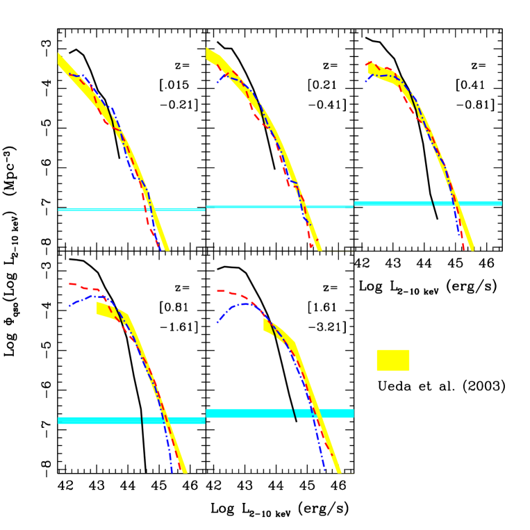
Figure 1: 2-10 keV X-ray LF. The lines are the predictions of the STD model (black solid line), DW model (red dashed line), AW model (blue dot-dashed line). The shaded region represents the Ueda et al (2003) estimate. The cyan horizontal bands give the limit below which the LF is affected by poor statistics in our run (equation 16)

In this section we compare the results of our model to observations of LFs and number counts in the hard-X, soft-X and optical bands, and to the statistics of remnant BHs at $z=0$. To best illustrate the constraints that can be obtained on the physical processes described above we show results for the three combination of parameters given in table 1 and introduced in section 2.7. The STD model refers to the standard choice of parameters presented in paper I, with the addition of the forced quenching procedure described in section 2.4. In this case quasar winds are not active ($f_{\rm qw}=0$). The resulting LFs for this model are always too steep (figures 1–4) though the $z=0$ BH – bulge relation is roughly reproduced (figure 6) for $M_{\rm B}\ga 10^{11}$ M_⊙. Within the range of parameters allowed by the constraints of galactic observables (see paper I and Fontanot et al. 2006b) we have found no way to have shallower LFs. On the other hand, the introduction of quasar winds allows us to improve the agreement with AGN data without influencing much the results on galaxies. The DW model includes drying winds as follows. In order to flatten the AGN LF the $\alpha_{\rm lowJ}$ exponent is set to 2, so that accretion is increased in the strong starbursts that give rise to big spheroids, and depressed in small bulges; in order to avoid a dramatic steepening of the BH – bulge relation at $z=0$, drying winds are introduced to limit the mass of the most massive BHs. In this case we use $f_{\rm lowJ}=0.03$ in place of the 0.003 value of STD. Another good combination of parameters (model AW) is found by allowing accreting winds (with $f_{\rm qw}=0.006$, $f_{\rm lowJ}=0.01$ and $f_{\rm centre}=0.002$) and setting $\Sigma_{\rm lim}=300$ M_⊙ pc^-2 (model AW); in this case both the starbursts induced in discs with a high gas surface density and the secondary accreting episodes stimulated by the quasar wind increase the activity of bright quasars even with $\alpha_{\rm lowJ}=1$,

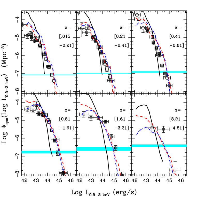
Figure 2: 0.5-2 keV X-ray LF. Lines refer to models as in figure 1. In all panels the empty circles and squares refer respectively to the observations of Miyaji et al. (2001) and Hasinger et al. (2005).

Figures 1, 2 and 3 show that the DW and AW models fit nicely (though maybe not in detail) the observed LFs of quasars in all the bands considered.

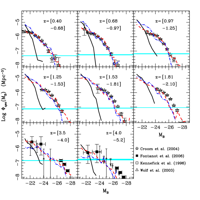
Figure 3: B-band LF. Lines refer to models as in figure 1. Data are taken from Kennefick et al. (1996), Wolf et al. (2003), Croom et al. (2004), Fontanot et al. (2006a), as indicated in the figure.

Figure 4 shows the same results in a different way. The predicted number density of AGNs in bins of bolometric luminosity is compared to the range of values inferred from observations (using mainly the analytic fit of the hard-X LFs of Ueda et al. 2003, Barger et al. 2003 and La Franca et al. 2005 for $z<3.5$, and the results of Fontanot et al. 2006a at $z>3.5$). The three models are all shown. It is clear that the DW and AW models reproduce nicely the evolution of the AGN population, with the number distributions peaking at lower redshift for lower luminosity. In other words, the downsizing or anti-hierarchical behavior of AGNs can be recovered in the context of the hierarchical $\Lambda$CDM cosmogony once feedback is properly modeled.

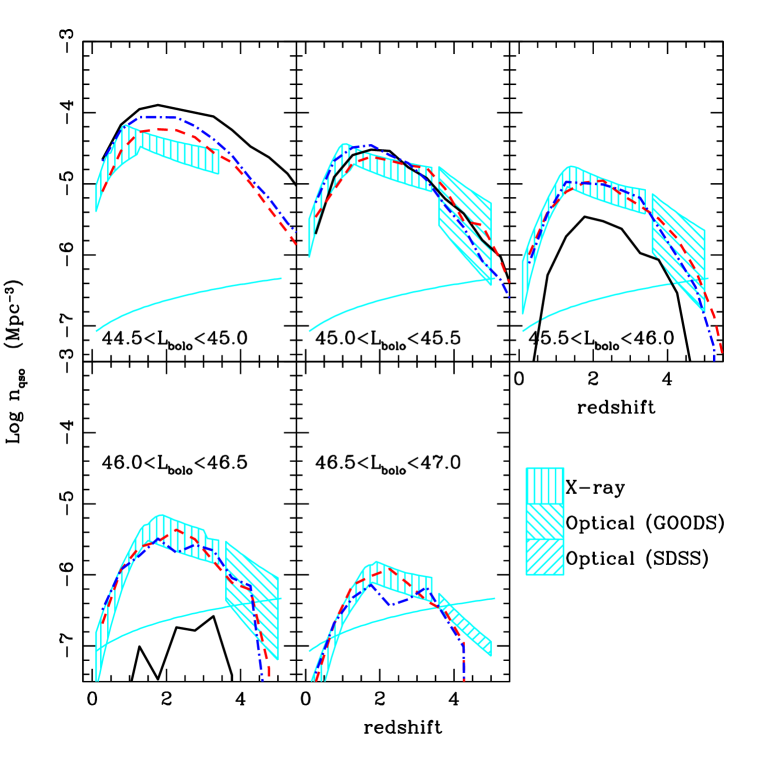
Figure 4: Evolution of the QSO number density with redshift in different bins of bolometric luminosity, estimated from X-ray (Ueda et al. 2003; Barger et al. 2003; La Franca et al. 2005) and optical (SDSS, Fan et al. 2003; GOODS, Fontanot et al. 2006a) surveys. Lines refer to models as in figure 1.

Similar results are obtained with the 150 Mpc box, though the statistical limit for the number density of objects (equation 16) is higher by a factor of 2.4, the decrease of the AGN activity at low redshift is marginally slower and the slight excess of faint AGNs at $z\sim 2$ is a bit larger. Clearly, some of these discrepancies can be absorbed by a further tuning of the parameters, which we deem worthless in this analysis.

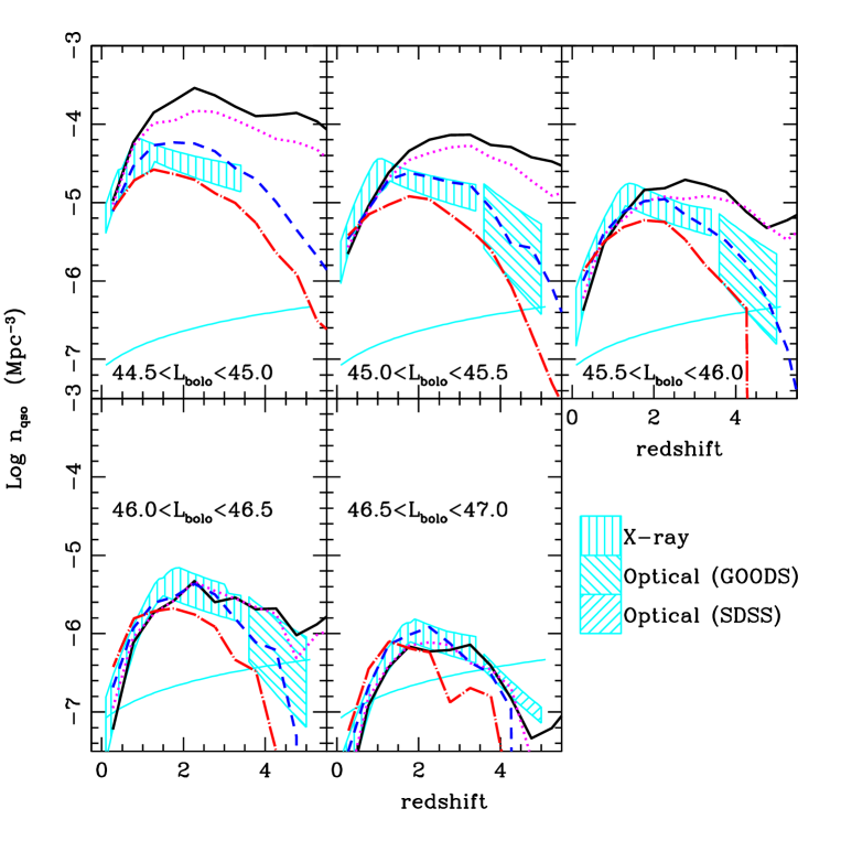
Figure 5: Evolution of the QSO number density for the DW model as a function of $\sigma_{0}$. The black solid line refers to $\sigma_{0}=0$ km s^-1, the magenta dotted line to $\sigma_{0}=30$ km s^-1, the blue dashed line to $\sigma_{0}=60$ km s^-1 (the best-fit value) , the red dot-dashed lines to $\sigma_{0}=90$ km s^-1.

From a much more detailed analysis of the parameter space we infer that the physical process at the origin of the downsizing of AGNs is the kinetic feedback active in star-forming bulges. This is shown in figure 5, where the DW model is shown with $\sigma_{0}$ values ranging from 0 to 90 km s^-1 (very similar results are obtained with the other models). Kinetic feedback causes a strong ejection of cold gas in small bulges, thus decreasing the number of faint AGNs without changing much the number of bright quasars. From this comparison we obtain a best-fit value for $\sigma_{0}$ of 60 km s^-1; this is the most effective way to constrain this parameter. It is also worth noticing in figure 5 the fundamental importance of the constraint coming from the abundance of high-$z$ AGNs in the GOODS fields (Cristiani et al. 2004; Fontanot et al. 2006a).

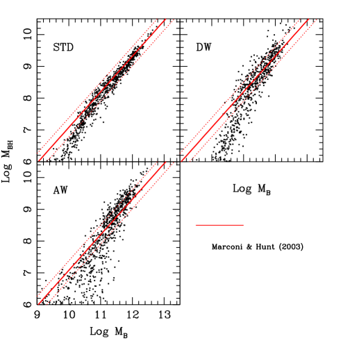
Figure 6: Predicted $M_{\rm B}-M_{\rm BH}$ relation at $z=0$ for STD, DW and AW models. The thick diagonal line gives the observed mean relation according to Marconi & Hunt (2003), the dotted lines highlight the observed scatter of 0.3 dex.

Figure 6 shows the BH – bulge relation at $z=0$ predicted by the models, while figure 7 shows the resulting mass function of BHs. All models, included STD, roughly reproduce the observed range of values for massive bulges ($M_{\rm B}\ga 10^{11}$ M_⊙), with some modest overestimate by the wind models (especially AW), while a steepening is predicted at smaller masses. This figure allows to make some important points. First, despite its fundamental importance in demonstrating the connection between AGNs and their host bulges, this relation is not after all a very strong constraint, as the three models give similar fits (for $M_{\rm B}>10^{11}$ M_⊙) despite their remarkably different performance in terms of LFs and number densities of objects. Second, the scatter of this relation is remarkably low in the STD model, and this suggests that the recipes given in section 2.4 are too simple and some source of scatter is needed. Intriguingly, quasar winds give roughly the correct amount of scatter, though they tend to give too many massive BHs at $z=0$. Third, BHs in small bulges are too small compared to observations. This very important point will be deepened below.

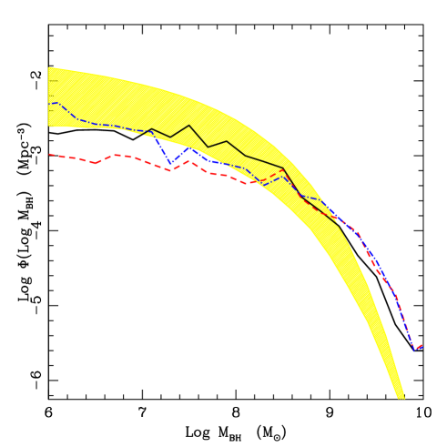
Figure 7: BH mass function at $z=0$ for the models. (lines refer to models as in figure 1), compared to the region allowed by the Shankar et al. (2004) and Marconi et al. (2004) estimates (shaded area).

3.1 X-ray number counts and background

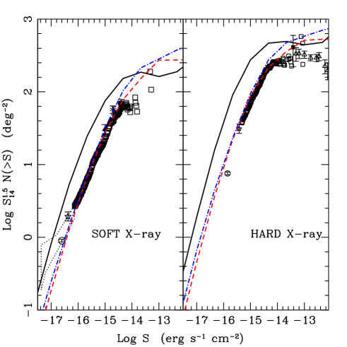
Figure 8: Cumulative Source Number Counts in X-ray bands. Left Panel: soft (0.5-2 keV). Estimates from Hasinger et al., (1993) (dotted region); Brandt et al., (2001) (empty star); Bauer et al., (2004) (empty circle); Hasinger (1998) (filled triangle); Zamorani, Mignoli & Hasinger (1999) (filled circle); Rosati et al. (2002) (empty squares). Right Panel: hard (2-10 keV). Estimates from Giommi et al., (2001) (empty triangles); Ogasaka et al. (1998) (filled square); Brandt et al., (2001) (empty star); Bauer et al., (2004) (empty circle); Rosati et al. (2002) (green empty squares). Lines refer to models as in figure 1

In order to strengthen the constraints on the AGN population we compare our model predictions to X-ray number counts (figure 8) in the soft and hard X-ray bands. Apart from some possible overestimate at the brightest fluxes, the fit to the data of the two wind models (DW and AW) is very good, while the STD model overestimates the counts by roughly a factor of three, and this is due to the overestimate of the faint end of the LFs.

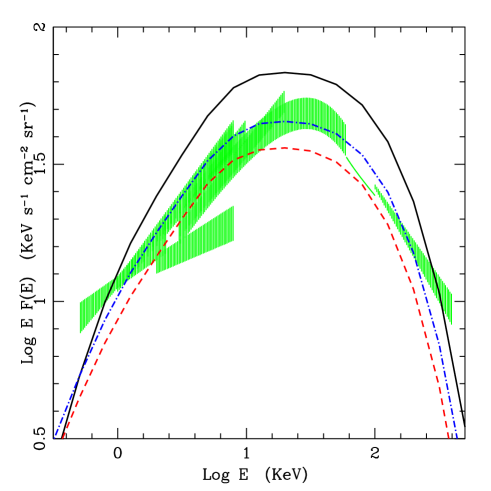
Figure 9: Reproduction of the X-ray background. Observations are highlighted by the shaded areas and are taken from Revnivtsev et al. (2003), Worsley et al. (2004), Georgantopoulos et al (1996), Vecchi et al. (1999), Lumb et al., (2002), De Luca & Molendi (2004), Kinzer et al., (1997), Gruber et al. (1992). Lines refer to models as in figure 1

Figure 9 shows the prediction for the X-ray background from 0.5 to 300 keV. The background predicted by the two wind models follows nicely the observed one, though the peak at $\sim 30$ keV is underpredicted by the DW model. This is in line with the results of La Franca et al. (2005), who claim a missing (though not dominant) population of Compton-thick AGNs, which is not included in this background synthesis that uses similar ingredients as their paper. This agreement shows that also the population of faint sources is roughly reproduced by the wind models.

3.2 More predictions

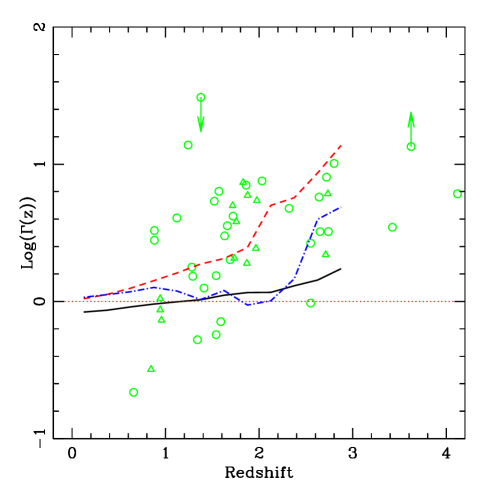
Figure 10: Evolution in redshift of the BH–bulge relation through the $\Gamma$ parameter (equation 20) for the three models. Lines refer to models as in figure 1. Data points are taken from Peng et al. (2006).

In order to quantify the amount of evolution in the BH-bulge relation we compare our model predictions with the results of Peng et al. (2006), who measured the evolution of the BH – bulge relation by defining the quantity $\Gamma(z)$:

$$\Gamma(z)=\frac{M_{\rm B}}{M_{\rm BH}}(z)/\frac{M_{\rm B}}{M_{\rm BH}}(z=0)$$ (20)

In figure 10 we present the average evolution of $\Gamma$ predicted by the three models, but only for the galaxies with $M_{\rm B}>2\times 10^{11}$, which safely lie on the relation. The model STD show some degree of evolution, which is due to the fact that, consistently with Croton (2006), the fraction of stars formed in bulges is higher at higher redshift, so that a higher fraction of gas can accrete on the BH. On the other hand, the wind models show a more pronounced increase of $\Gamma$ with redshift, in better agreement with Peng et al. (2006). This was anticipated in Monaco & Fontanot (2005), who showed that if more mass is allowed to flow onto the BH until the winds limits further accretion, then the mass assembly of massive BHs is anticipated. This can help in reconciling the presence of bright quasars at high redshift, when very massive galaxies were not yet assembled.

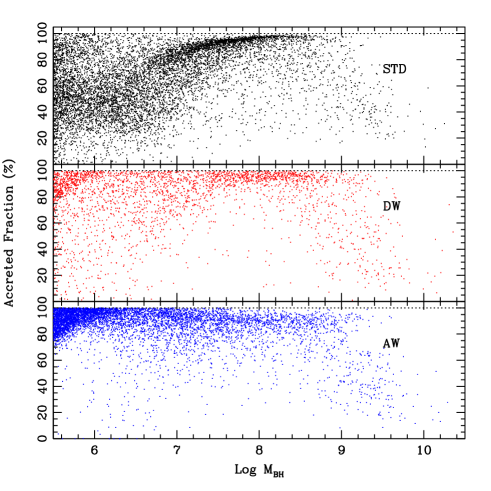
Figure 11: Scatter-plot of the predicted fraction of BH mass acquired by accretion as a function of BH mass, for BHs in $z=0$ galaxies. The three panels give the results of the STD (upper), DW (mid) and AW (lower) model.

Regarding the mechanisms responsible for the assembly of BHs, we find that the bulk of BH mass is gained from accretion. Figure 11 shows the fraction of mass acquired by accretion (the rest is acquired by mergers) as a function of BH mass for the BHs found in $z=0$ galaxies, according to the three models. We notice that merging is significant for the most massive BHs, which reside in the most massive galaxies that experience complex merger histories (see, e.g., De Lucia et al. 2006; De Lucia & Blaizot 2006). We also notice that quasar winds, especially the accreting winds, increase the amount of mass acquired by accretion.

Another important prediction is the average accretion rate of BHs in units of the Eddington rate. This quantity is needed to relate the accretion history of AGNs, estimated from the LFs, to the local BH mass function. As each accretion event is subdivided by our model into many sub-events, one per integration interval, we show this quantity averaged over bins of bolometric luminosity and redshift and weighted by the width of the time bin. Figure 12 shows the results for the STD, DW and AW models. While the STD rates are very low, especially for the highest accretion rates, the Eddington ratios of the other models are rather high at high redshift and decrease at low redshift, especially for low AGN luminosities. This prediction is compared with the observational results of Kollmeier et al. (2006), based on a sample of 407 AGNs from the AEGIS survey, with BH masses estimated through a combination of line widths and continuum luminosities; the agreement is reasonably good, though Eddington ratios tend to be higher than the data at high redshift. This shows that the reason why the STD model fails to produce bright quasars relies in the low accretion rates stimulated by star formation, while the main effect of winds is to force massive BHs to accrete at high rates. A similar prediction was given in Kauffmann & Haehnelt (2000), based on a parametric description of the accretion timescale. Our more refined modeling allows us to propose that this behaviour can be obtained only by inserting quasar-triggered galaxy winds. Finally, the predicted dependence of the Eddington ratios on redshift and bolometric luminosity can be useful to relate the accretion history of BHs to the observed mass function of remnant BHs at $z=0$.

4 Discussion

The main message of this paper is that it is possible to include accreting BHs in a complete galaxy formation model like morgana so as to reproduce the main constraints on the AGN population from the optical to the hard X-ray. However, this good agreement is reached at the cost of meddling with the very uncertain physics of quasar-triggered galactic winds. By presenting two different good solutions, both based on motivated and plausible choices on how to insert quasar winds, we intend to stress that the parameter space is so wide, even in the restricted version presented here, that it is not possible to constrain in a unique way the complex processes at play simply by reproducing the statistical properties of the AGN population.

The second message of the paper is that, notwithstanding their non-uniqueness, the only acceptable solutions we find are based on quasar winds. As clear in figure 12, the role of quasar winds is to force a high accretion rate for the massive BHs and reproduce the trend of increasing Eddington ratio with bolometric luminosity, in better agreement with data. Given the uncertainties on the physics of these events, it is possible to use this result as a suggestive clue on the role of winds but not as a strong evidence of their necessity. This caution is confirmed by the fact that most papers cited in the Introduction are able to reproduce bright quasars without advocating any such mechanism. However, there is a deep difference between our model, where the accumulation of low-$J$ gas is connected to star formation, and most other models where some cold gas is produced at a triggering event (mergers if not flybies) and accreted at an arbitrarily specified fraction of the Eddington rate. In this regard our model can be directly compared only to that of Granato et al. (2004), who proposed a very similar modeling of the accretion onto the BH, but used a lower value of their parameter equivalent to $f_{\rm lowJ}$; in their case the wind takes place when the star-formation episode has consumed nearly all the gas, and their winds do not limit strongly the BH mass. Their model should then be more similar to our unsuccessful STD model. But the real difference between their approach and morgana relies in the treatment of star formation and feedback; in particular, they assume that the formation of an elliptical takes place in a single episode and that the cooling gas goes to the bulge, while in our model and in the same context the cooling gas would settle on a disc until it loses angular momentum through bar instabilities, mergers or feedback (see the discussion on the role of $\Sigma_{\rm lim}$ in section 2.2). As a consequence, in morgana many of the stars that end up in bulges are formed in discs and do not contribute to the loss of angular momentum of gas (this is the main reason for the scatter in the BH – bulge relation). Our higher values of $f_{\rm lowJ}$ allow to have stronger accretion events and higher BH masses at high redshift, but then a limiting mechanism, like quasar winds, is necessary to avoid to overshoot heavily the BH – bulge relation. In this regard, the modest overestimate of large BH masses by the DW and AW models could be fixed by a more careful study of the parameter space, but we find hints that winds are a key ingredient to achieve agreement with many observables.

Our model is also comparable to that of Cattaneo et al. (2005), who relate the accretion rate to the star-formation rate in a similar way as equation 10, with their equivalent of the $\alpha_{\rm lowJ}$ parameter equal to 1.5. Unfortunately, their relatively small box (100 Mpc$/h$ with $256^{3}$ particles) does not allow to reach strong conclusion on the prediction of their model for bright quasars.

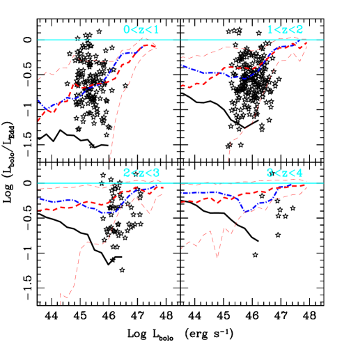
Figure 12: Predicted average accretion rates in units of Eddington; thick lines refer to models as in figure 1. Thin lines represent the variance of the DW model, which is representative also for the other models. Stars refer to data from Kollmeier et al. (2006).

The third message is that kinetic feedback in star-forming bulges is a very good candidate for the main mechanism responsible for the downsizing of AGNs. This point however needs some discussion. An overall good agreement between models (DW or AW) and data is obtained only for $M_{\rm B}\ga 10^{11}$ M_⊙ and $M_{\rm BH}\ga 10^{8}$ M_⊙; at smaller values the BH – bulge relation steepens considerably, especially in the DW model. We think that this discrepancy points to an intrinsic problem of morgana that is shared with most other galaxy formation models. As shown in paper I, the predicted stellar mass function of bulge-dominated galaxies does not have a broad peak at $\sim 10^{10}$ M_⊙, as suggested by observations, but presents a power-law tail of small objects which is just below that of discs; this problem is shared, for instance, by the model of Croton et al. (2006). Recently, Fontana et al. (2006), based on the GOODS-MUSIC sample (Grazian et al. 2006), reconstructed the stellar mass function of galaxies up to $z\sim 4$ and compared their results with N-body and semi-analytic models including morgana. All the models were found to overpredict the number density of small galaxies at $z\sim 1$; many of these galaxies are the likely progenitors of small bulges. Similar results are obtained with the Garching model (De Lucia, private communication). The mechanism of kinetic feedback can suppress effectively star formation in small bulges, but, as mentioned above, cannot hamper stars that form in discs to get into bulges. As a consequence, the formation of BHs is suppressed but the number of bulges is not, and the BH – bulge relation steepens (remarkably, the steepening is slightly less evident in the AW case, where the discs with high gas surface density are transformed into bulges). In other words, a good fit of the number of AGNs and an overestimate of the number of bulges can only be compatible with a steep BH – bulge relation.

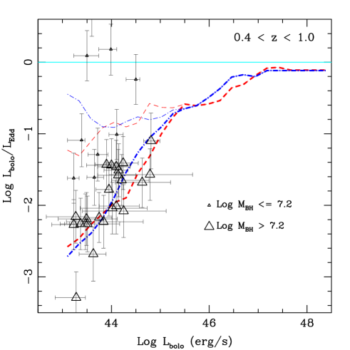
Figure 13: Predicted Eddington ratios as a function of the bolometric luminosity for BHs more massive than $10^{7.2}$ M_⊙ (thick lines, red dashed for the DW model, blue dot-dashed for the AW model) and for all BHs (thin lines, styles as above). Data are from Ballo et al. (2006), large points refer to BHs more massive than $10^{7.2}$ M_⊙, smaller points to smaller BHs. The thick lines should be compared with the large points, the thin lines with all the points.

The excess of small bulges is slightly over-corrected by kinetic feedback, in that the resulting BH mass function is low at small masses (figure 7). This over-correction can be explained as follows: kinetic feedback, which is applied at a rather high level, limits the accretion on small BHs ($M_{\rm BH}\simeq 10^{6}-10^{7}$ M_⊙), but these BHs are anyway hosted in larger bulges (figures 6 and 10), so they are likely to have access to larger amounts of gas; then, a given (small mass) BH can give rise to more (low-luminosity) AGN activity than desired. The constraint on the total accretion leads then to a further underestimate of BH masses. But if the small BHs are to provide the correct amount of AGN activity, they should accrete on average at a higher rate than observed. To test this idea we compare our predictions with the observations of Ballo et al. (2006), who estimated stellar masses, bolometric luminosities and BH masses (based on the BH – bulge relation at $z=0$) for a hard X-ray-selected sample of faint AGNs hosted in galaxies at $0.4<z<1$. Figure 13 shows the Eddington fraction of the DW and AW models compared to the Ballo et al. (2006) data for $M_{\rm BH}>1.6\times 10^{7}$ M_⊙ and for all BH masses. In particular, the thick lines show model predictions with the same mass limit; these are in very good agreement with the corresponding observational points (the larger triangles). This means that the accretion rate of these BHs is correctly reproduced by the model. This result does not depend on the details of the quenching of cooling flows by AGN feedback, as the involved BH masses are rather small; indeed, identical results are obtained in the higher resolution box with the standard quenching procedure. Besides, the accretion rate of all BHs (thin lines), which is dominated by the smaller objects, is tendentially larger than observed (the thin lines must be compared with both large and small triangles). This trend is not very strong, and could be due to a lack of small BHs in the dataset; however, as discussed in the Ballo et al. (2006) paper, the hard X-ray selection makes this possible bias weak if not absent. This comparison then confirms that, to compensate for the excess of small bulges, our model generates too few small BHs ($M\la 10^{7}$ M_⊙) that, being hosted in relatively larger bulges, accrete at a higher rate. The kinetic feedback mechanism remains then a very good candidate for downsizing AGNs, but the value proposed here of 60 km s^-1 is probably overestimated.

The discrepancy described above points to some missing feedback mechanism active at high redshift able to downsize the small star-forming discs in the same way as kinetic feedback does for the small bulges. Bulge formation by feedback, explained in section 2.2, helps but does not solve the problem, so other mechanisms are required.

Other authors have obtained good agreement between the prediction of similar semi-analytic models and data in terms of the downsizing of the AGN population, so it is worth wondering if other mechanisms than kinetic feedback can give similarly good results. In the case of Granato et al. (2001, 2004), the downsizing is obtained by delaying the shining of quasars, as originally suggested by Monaco et al. (2000). This delay is justified by stellar feedback, but the model does not make a distinction between thermal and kinetic feedback. Menci et al. (2003, 2004, 2006; see also Vittorini et al. 2006) obtain similarly good results, although the level of predicted downsizing may be slightly less than that required by data (Menci, private communication). In their case the downsizing is obtained by stellar feedback (parameterized as usual with a $\beta$ coefficient which is a power-law of the disc velocity) and by the insertion of galaxy-galaxy interactions as a further trigger of AGN activity, a mechanism which penalizes the small satellites. Similarly, Cattaneo et al. (2005) with a standard feedback recipe and an accretion rate similar to equation 10 (but without reservoir) obtain a roughly good match to the optical LF of quasars. In all these cases stellar feedback is treated in a simple and parametric way. As shown and discussed in Monaco (2004a) and Paper I, feedback in discs can lead to the reheating of an amount of cold gas roughly equal to the star-formation rate, which means $\beta\simeq 1$, so the only way to have more cold gas ejected to the halo is to accelerate it more than heating it. We are then rough agreement with the papers mentioned above in stating that the suppression of faint AGNs at high redshift is due to stellar feedback, but our more refined modeling allows us to draw stronger conclusions on the details of the physical mechanism at play.

5 Conclusions

This paper belongs to a series devoted to presenting morgana, a new model for the joint formation and evolution of galaxies and AGNs, and is focused on the role of feedback in shaping the observed properties of AGNs and their relation with galaxies. Our analysis confirms that models based on the $\Lambda$CDM cosmogony are able to roughly reproduce at the same time both the properties of AGNs (presented here) and the properties of galaxy populations (presented in paper I, Fontana et al. 2006 and Fontanot et al. 2006b).

This model has been extended, through a careful modeling of AGN SEDs, to predict many QSO properties, especially in the X-rays. It reproduces nicely LFs and number counts in the soft and hard X-ray bands, and the measured background from 0.5 to 300 keV, with a possible underestimate of the peak which confirms the claim for a significant though not dominant population of Compton-thick sources. This implies that the bulk of AGN accretion is roughly reproduced.

The agreement between model and data allows us to draw these conclusions.

Quasar triggered winds are necessary in our model to reproduce the number density of bright quasars. The parameter space of quasar winds is discouragingly wide; within a very limited sub-space, characterized by “only” six parameters, we find two good solutions, which is a clear sign that our knowledge on the physics of accretion onto BHs and their interaction with galaxies is still too poor to draw firm conclusions. In any case, the idea that quasar winds are a necessary ingredient of galaxy formation is worth pursuing. The two wind solutions that we propose are based on the same triggering criterion for the quasar wind, requiring that (i) the accretion rate is high enough to perturb the ISM, (ii) the gas mass to remove is not too high, (iii) the AGN is accreting in a radiatively efficient mode. The first solution is based on a tilt of the relation between bulge star-formation rate and loss rate of angular momentum, compensated by “drying winds”, where the kinetic energy injected by the central engine causes a complete removal of ISM from the host bulge. The second solution is based on the “accreting wind” mechanism proposed by Monaco & Fontanot (2005), where the wind is generated throughout the ISM, so that a fraction of the cold gas is compressed to the center and stimulates further accretion. A good fit of the AGN LFs is then obtained by assuming, as explained in paper I, that discs with high gas surface density lose angular momentum (and then become bulges) because of the expected change in the feedback regime (Monaco 2004a) and the consequent increase of the velocity dispersion of clouds (as observed by Förster Schreiber et al. 2006).

We propose that kinetic feedback in star-forming bulges is a very good candidate for downsizing the AGN population. Indeed, the high velocity dispersion of cold gas in star-forming bulges can lead to a massive removal of ISM, leading to a suppression of less luminous AGNs at high redshift, while larger elliptical galaxies can retain their gas more easily. At lower redshift larger BHs may accrete at lower rates, giving rise to the low-luminosity population dominating the X-ray background.

We make the following predictions: (i) the BH-bulge relation is already in place at high redshift, though high BH masses in relatively small bulges may be found at $z>2$ if quasar winds are active; (ii) the Eddington ratios of accreting BHs depend both on redshift and bolometric luminosity, with low values for the faint AGNs at $0<z<1$ that give the bulk of the hard X-ray background (consistent with Ballo et al. 2006); (iii) most BH mass is acquired through accretion more than through mergers, especially if quasar-triggered winds are switched on.

There is an important point of discrepancy between our model and data, in that the predicted BH – bulge relation at $M_{\rm B}<10^{11}$ M_⊙, or $M_{\rm bh}<10^{8}$ M_⊙, is significantly steeper than observed; in the same mass range the predicted mass function of BHs is too low. To our understanding, this is connected to a known excess of small bulges with respect to observations (see paper I) and to the excess of small-mass galaxies predicted by most (N-body or semi-analytic) models at $z\sim 1$ (Fontana et al. 2006). We have tested this idea by comparing our model predictions of the Eddington ratios of faint AGNs at $0.4<z<1$ with the data of Ballo et al. (2006); while the agreement is excellent for $M>1.6\times 10^{7}$ M_⊙, smaller BHs accrete at a higher rate than observed, and this compensates for the lack of smaller BHs. This discrepancy highlights that while kinetic feedback is efficient in downsizing AGNs by quenching the star formation in bulges, stars in small ellipticals may be born in discs, so that another mechanism is needed to produce the required level of downsizing of bulges.

In conclusion, in developing this work we have gained interesting insight into the complex problem of the cosmological rise of AGNs, highlighting two promising astrophysical mechanism (kinetic feedback in star-forming bulges and quasar-triggered galaxy winds) and the need for a third, unknown one to improve the downsizing of elliptical galaxies. However, our poor understanding of the underlying physics hampers more robust conclusions. This demonstrates once again that the field of joint galaxy and AGN formation is observationally-driven and we need strategies to single out the physical mechanisms at play. In particular, the main degrees of freedom in the theory are related to the connection between BH accretion and star formation, which can be constrained by estimating accretion rates, star-formation rates and BH masses in active galaxies; to the quasar-triggered winds, which can be constrained by observing warm and cold absorbers or Lyman-$\alpha$ blobs associated to quasars; and finally to the nature of stellar feedback, which can be constrained by detailed observations of starburst galaxies. The next generation of telescopes will provide suitable tools to assess these topics.

References

- (1) Barger, A.J., Cowie, L.L., Mushotzky, R.F., Yang, Y., Wang, W.-H., Steffen, A.T., Capak, P., 2005, AJ, 129, 578
- (2) Ballo, L., Cristiani, S., Fasano, G., et al., 2006, submitted to ApJ
- (3) Bauer, F.E., Alexander, D.M., Brandt, W.N., Schneider, D.P., Treister, E., Hornschemeier, A.E., Garmire, G.P., 2004, AJ, 128, 2048
- (4) Benson, A.J., Bower, R.G., Frenk, C.S., Lacey, C.G., Baugh, C.M., Cole, S., 2003, ApJ, 599, 38
- (5) Bower, R.G., Benson, A.J., Malbon, R., Helly, J.C., Frenk, C.S., Baugh, C.M., Cole, S., Lacey, C.G., 2006, MNRAS, 370, 645
- (6) Brandt, W., Alexander, D.M., Hornschemeier, A.E., et al., 2001, AJ, 122, 2810
- (7) Bromley J.M., Somerville R.S., Fabian A.C., 2004, MNRAS, 350, 456
- (8) Cattaneo A., 2001, MNRAS, 324, 128
- (9) Cattaneo, A., Blaizot, J., Devrient, J., Guiderdoni, B., 2005, MNRAS, 364, 407
- (10) Cavaliere, A., Padovani, P., 1988, ApJ, 333, L33
- (11) Cavaliere, A., Vittorini, V., 2000, ApJ, 543, 599
- (12) Cavaliere, A., Vittorini, V., 2002, ApJ, 570, 114
- (13) Ciotti, L., Ostriker, J.P., 1997, ApJ, 487, L105
- (14) Cowie, L.L., Songaila, A., Hu, E.M., Cohen, J.G., 1996, AJ, 112, 839
- (15) Cristiani, S., Vio, R., 1990, A&A, 227, 385
- (16) Cristiani, S., Alexander, D.M., Bauer, F., et al., 2004, ApJL, 600, 119
- (17) Croom, S.M., Smith, R.J., Boyle, B.J., Shanks, T., Miller, L., Outram, P.J., Loaring, N.S., 2004, MNRAS, 349, 1397
- (18) Croton, D.J., 2006, MNRAS, 369, 1808
- (19) Croton, D.J., Springel, V., White, S.D.M., et al., 2006, MNRAS, 365, 11
- (20) Dalla Vecchia, C., Bower, R.G., Theuns, T., Balogh, M.L., Mazzotta, P., Frenk, C.S. 2004, MNRAS, 355, 995
- (21) De Luca A., Molendi S., 2004, A&A, 419, 837
- (22) De Lucia, G., Springel, V., White, S.D.M., Croton, D., Kauffmann, G., 2006, MNRAS, 366, 499
- (23) De Lucia, G., Blaizot, J., 2006, submitted to MNRAS (astro-ph/0606519)
- (24) Dib, S., Bell, E., Burkert, A., 2006, ApJ, 638, 797
- (25) Di Matteo, T., Croft, R.A.C., Springel, V., Hernquist, L., 2003, ApJ, 593, 56
- (26) Di Matteo, T., Springel, V., Hernquist, L., 2005, Nature, 433, 604
- (27) D’Odorico, V., Cristiani, S., Romano, D., Granato, G.L., Danese, L., 2005 MNRAS, 351, 976
- (28) Dunlop J.S., McLure R.J., Kukula M.J., Baum S.A., O’Dea C.P., Hughes D.H., 2003, MNRAS, 340, 1095
- (29) Elvis, M., Wilkes, B.J., McDowell, J.C. et al., 1994, ApJS, 95, 1
- (30) Fabian A.C., 1999, MNRAS, 308, 39
- (31) Fan, X., Strauss, M.A., Schneider, D.P., et al. 2003, AJ, 125, 1649
- (32) Fabian, A.C., Sanders, J.S., Taylor, G.B., Allen, S.W., Crawford, C.S., Johnstone, R.M., Iwasawa, K., 2006, MNRAS, 366, 417
- (33) Fontana, A., Salimbeni, S.,Grazian, A., et al., 2006, A&A, in press (astro-ph/609068)
- (34) Fontanot, F., Cristiani, S., Monaco, P. et al., 2006a, A&A, in press (astro-ph/0608664)
- (35) Fontanot, F., Monaco, P., Silva, L., et al., 2006b, in preparation
- (36) Förster Schreiber, N.M., Genzel, R., Lehnert, M.D., et al., 2006, ApJ, in press
- (37) Georgantopoulos, I., Steward, G.C., Shanks, T., Boyle, B.J., Griffiths, R.E., 1996, MNRAS, 280, 276
- (38) Giommi P., Perri M., Fiore F., 2000, A&A, 362, 799
- (39) Granato G.L., Silva L., Monaco P., Panuzzo P., Salucci P., De Zotti G., Danese L., 2001, MNRAS, 324, 757
- (40) Granato G.L., De Zotti G., Silva L., Bressan A., Danese L., 2004, ApJ, 600, 580
- (41) Grazian, A., Fontana, A., de Santis, C., et al., 2006, A&A, 449, 951
- (42) Gruber D.E., 1992, In: Barcons X., Fabian A.C., (eds.), The Proocedings of: The X-ray Background. Cambridge Univ. Press, Cambridge, p.44
- (43) Haehnelt, M.G., Natarajan, P., Rees, M.J., 1998, MNRAS, 300, 817
- (44) Haiman, Z., Ciotti L., Ostriker J.P., 2004, ApJ, 606, 763
- (45) Hamann, F., Ferland, G., 1999, ARA&A, 37, 487
- (46) Häring N., Rix H.W., 2004, ApJ, 604, 89
- (47) Hasinger G., 1998, Astron. Nacht., 319, 37
- (48) Hasinger, G., Miyaji, T., Schmidt, M., 2005, A&A, 441, 417
- (49) Hasinger, G., Burg, R., Giacconi, R., Hartner, G., Schmidt, M., Trumper, J., Zamorani, G., 1993, A&A, 275, 1
- (50) Hopkins, P.F., Hernquist, L., Cox, T.J., Di Matteo, T., Robertson, B., Springel, V., 2006, ApJS, 163, 1
- (51) Kang, X., Jing, Y.P., Silk, J., 2006, ApJ, accepted (astro-ph/0601685)
- (52) Kauffmann G., Haehnelt M.G., 2000, MNRAS, 311, 576
- (53) Kazantzidis, S., Mayer, L., Colpi, M., Madau, P., Debattista, V.P., Wadsley, J., Stadel, J., Quinn, T., Moore, B., ApJ, 623, L67
- (54) Kennefick, J.D., Djorgovski, S.G., Meylan, G., 1996, AJ, 111, 1816
- (55) Kennicutt, R.C., 1989, ApJ, 344, 685
- (56) Kinzer, R.L., Jung, G.V., Gruber, D.E., Matteson, J.L., Peterson, L.E., 1997, ApJ, 475, 361
- (57) Kollmeier, J.A., Onken, C.A., Kochanek, C.S. et al., 2006, ApJ, 648, 128
- (58) Kormendy J., Richstone D., 1995, ARA&A, 33, 581
- (59) Kriss G.A., Davidsen A., Zheng W., Lee G., 1999, ApJ, 527, 683
- (60) La Franca, F., Fiore, F., Comastri, A., et al., 2005, ApJ, 635, 864
- (61) Lumb D.H., Warwick R.S., Page M., De Luca A., 2002, A&A, 389, 93
- (62) Madau, P., Haardt, F., Rees, M.J., 1999, ApJ, 514, 648
- (63) Magorrian J., Tremaine S., Richstone D. et al., 1998, ApJ, 115, 2285
- (64) Mahmood A., Devriend J.E.G., Silk J., 2005, MNRAS, 359, 1363
- (65) Malbon, R.K., Baugh, C.M., Frenk, C.S., Lacey, C.G., 2006, submitted to MNRAS (astro-ph/0607424)
- (66) Marconi A., Hunt L.K., 2003, ApJ, 589, 21
- (67) Marconi, A., Risaliti, G., Gilli, R., Hunt, L.K., Maiolino, R., Salvati, M. 2004, MNRAS, 351, 169
- (68) Matteucci, F., Padovani, 1993, ApJ, 419, 485
- (69) Matteucci, F., 1994, A&A, 288, 57
- (70) McNamara, B.R., Nulsen, P.E.J., Wise, M.W., Rafferty, D.A., Carilli, C., Sarazin, C.L., Blanton, E.L., 2005, Nature, 433, 45
- (71) Menci, N., Cavaliere, A., Fontana, A., Giallongo, E., Poli, F., Vittorini, V., 2003, ApJ, 587, L63
- (72) Menci, N, Fiore, F., Perola, G.C, Cavaliere, A., 2004, ApJ, 606, 58
- (73) Menci, N., Fontana, A., Giallongo, E., Grazian, A., Salimbeni, S., 2006, submitted to ApJ
- (74) Merloni, A., 2004, MNRAS, 353, 1035
- (75) Merloni, A., Heinz, S., Di Matteo, T. 2003, MNRAS, 345, 1057
- (76) Miyaji T., Hasinger G., Schmidt M., 2001, A&A, 369, 49
- (77) Mo, H.J., Mao, S., White, S.D.M., 1998, MNRAS, 295, 319
- (78) Monaco, P., 2004a, MNRAS, 352, 181
- (79) Monaco, P., 2004b, MNRAS, 354, 151
- (80) Monaco, P., 2006, MmSAI, 77, 678
- (81) Monaco, P., Salucci, P., Danese, L., 2000, MNRAS, 311, 279
- (82) Monaco, P., Theuns, T., Taffoni, G., Governato, F., Quinn, T., Stadel, J., 2002a, ApJ, 564, 8
- (83) Monaco, P., Theuns, T., Taffoni, G., 2002, MNRAS, 331, 587
- (84) Monaco, P., Fontanot, F., 2005, MNRAS, 359, 283
- (85) Monaco, P., Fontanot, F., Taffoni, G., 2006, submitted to MNRAS (Paper I)
- (86) Mori M., Ferrara A., Madau P., 2002, ApJ, 571, 40
- (87) Morrison, R., McCammon, D., 1983, ApJ, 270, 119
- (88) Murray, N., Quataert E., Thompson T.A., 2005, ApJ, 618, 569
- (89) Ogasaka Y., Kii T., Ueda Y., et al., 1998, Astron. Nacht., 319, 47
- (90) Papovich, C., Moustakas, L.A., Dickinson, M., et al., 2006, ApJ, 640, 92
- (91) Peng, C.Y., Impey, C.D., Rix, H.W., Kochanek, C.S., Keeton, C.R., Falco, E.E., Lehar, J., McLeod, B.A., 2006, (astro-ph/0603248)
- (92) Quilis, V., Bower, R.G., Balogh, M.L., 2001, MNRAS, 328, 1091
- (93) Renzini, A., 2004, in eds. J.S. Mulchaey, A. Dressler, A. Oemler 2004, Clusters of Galaxies: Probes of Cosmological Structure and Galaxy Evolution. Carnegie Observatories Astrophysics Series. Pag 261
- (94) Revnivtsev, M., Gilfanov, M., Sunyaev R., Jahoda K., Markwardt C., 2003, A&A, 411, 329
- (95) Risaliti, G., Elvis, M., 2005, ApJ, 629, L17
- (96) Romano, D., Silva, L., Matteucci, F., Danese, L., 2002, MNRAS, 334, 444
- (97) Rosati, P. Tozzi, P., Giacconi, R., et al., 2002, ApJ, 566, 667
- (98) Ruszkowski, M., Brüggen, M., Begelman, M.C., 2004, ApJ, 615, 675
- (99) Salucci P., Szuszkiewicz E., Monaco P., Danese L., 1999, MNRAS, 307, 637
- (100) Shankar F., Salucci P., Granato G.L., De Zotti G., Danese L., 2004, MNRAS, 354, 1020
- (101) Sijacki, D., Springel, V., 2006, MNRAS, 366, 397
- (102) Silk J., Rees M.J., 1998, A&A, 331, 1
- (103) Simpson, C., 2005, MNRAS, 360, 565
- (104) Soltan, A., 1982, MNRAS, 200, 115
- (105) Spergel, D.N., Bean, R., Doré, O., et al., 2006, submitted to ApJ (astro-ph/0603449)
- (106) Sutherland R., Dopita M., 1993, ApJS, 88, 253
- (107) Springel, V., Di Matteo, T., Hernquist, L., 2005, MNRAS, 361, 776
- (108) Taffoni, G., Mayer, L., Colpi, M., Governato, F., 2003, MNRAS, 341, 434
- (109) Taffoni, G., Monaco, P., Theuns T., 2002, MNRAS, 333, 623
- (110) Thomas, D., 1999, MNRAS, 306, 655
- (111) Treu, T., Ellis, R.S., Liao, T.X., van Dokkum, P.G., Tozzi, P., Coil, A., Newman, J., Cooper, M.C., Davis, M., 2005, ApJ, 633, 174
- (112) Ueda Y., Akiyama M., Ohta K., Miyaji T., 2003, ApJ, 598, 886
- (113) Umemura M., 2001, ApJ, 560, L29
- (114) Vecchi A., Molendi S., Guainazzi M., Fiore F., Parmar A.N., 1999, A&A, 349, 73
- (115) Vignali C., Brandt W.N., Schneider D.P., 2003, ApJ, 125, 433
- (116) Vittorini, V., Shankar, F., Cavaliere, A., 2005, MNRAS, 363, 1367
- (117) Voit, G.M., Donahue, M., 2005, ApJ, 634, 955
- (118) Volonteri, M., Haardt, F., Madau, P., 2003, ApJ, 582, 559
- (119) Yu Q., Tremaine S., 2002, MNRAS, 335, 965
- (120) Wolf, C., Wisotzki, L., Borch, A., Dye, S., Kleinheinrich, M., Meisenheimer, K., 2003, A&A, 408, 499
- (121) Worsley M.A., Fabian A.C., Barcons X., Mateos S., Hasinger G., Brunner H., 2004, MNRAS, in press
- (122) Wu, K.K.S., Fabian, A.C., Nulsen, P.E.J., 2001, MNRAS, 318, 889
- (123) Zamorani, G., Henry, J.P., Maccacaro, T., et al., 1981, ApJ, 245, 357
- (124) Zamorani, G., Mignoli, M., Hasinger, G., et al., 1999, A&A, 346, 731
- (125) Zanni, C., Murante, G., Bodo, G., Massaglia, S., Rossi, P., Ferrari, A., 2005, A&A, 429, 399