Mean-field concept and direct numerical simulations of rotating magnetoconvection and the geodynamo

Abstract

Mean-field theory describes magnetohydrodynamic processes leading to large-scale magnetic fields in various cosmic objects. In this study magnetoconvection and dynamo processes in a rotating spherical shell are considered. Mean fields are defined by azimuthal averaging. In the framework of mean-field theory, the coefficients which determine the traditional representation of the mean electromotive force, including derivatives of the mean magnetic field up to the first order, are crucial for analyzing and simulating dynamo action. Two methods are developed to extract mean-field coefficients from direct numerical simulations of the mentioned processes. While the first method does not use intrinsic approximations, the second one is based on the second-order correlation approximation. There is satisfying agreement of the results of both methods for sufficiently slow fluid motions. Both methods are applied to simulations of rotating magnetoconvection and a quasi-stationary geodynamo. The mean-field induction effects described by these coefficients, e.g. the $\alpha$-effect, are highly anisotropic in both examples. An $\alpha^{2}$-mechanism is suggested along with a strong $\gamma$-effect operating outside the inner core tangent cylinder. The turbulent diffusivity exceeds the molecular one by at least one order of magnitude in the geodynamo example. With the aim to compare mean-field simulations with corresponding direct numerical simulations, a two-dimensional mean-field model involving all previously determined mean-field coefficients was constructed. Various tests with different sets of mean-field coefficients reveal their action and significance. In the magnetoconvection and geodynamo examples considered here, the match between direct numerical simulations and mean-field simulations is only satisfying if a large number of mean-field coefficients are involved. In the magnetoconvection example, the azimuthally averaged magnetic field resulting from the numerical simulation is in good agreement with its counterpart in the mean-field model. However, this match is not completely satisfactory in the geodynamo case anymore. Here the traditional representation of the mean electromotive force ignoring higher than first-order spatial derivatives of the mean magnetic field is no longer a good approximation.
Keywords: Magnetohydrodynamics; Mean-Field Theory; Dynamo Coefficients; Magnetoconvection; Geodynamo

1 Introduction

Large-scale cosmic magnetic fields as the Earth’s, the solar and the galactic magnetic fields are maintained by hydromagnetic dynamos (e.g. Weiss, 2002). However, global computational dynamo models simulate only the geodynamo resonably well, while it remains difficult to tackle the stellar or galactic dynamo problem in this way. Despite the increasing computational power, a direct numerical treatment of the governing equations is not yet feasible in the latter cases, because of the huge range of spatial and temporal scales needed to be resolved there (Tobias, 2002; Weiss and Tobias, 2000; Shukurov, 2002). First attempts of global MHD simulations have been carried out by Gilman (Gilman and Miller, 1981; Gilman, 1983) adopting the Boussinesq approximation and later by Glatzmaier (Glatzmaier, 1984, 1985) using an anelastic model. Both aimed at modelling the solar dynamo. Though cyclic dynamo solutions were obtained in some cases, the models exhibited a wrong poleward migration of the magnetic field (Glatzmaier, 1985). In a recent attempt, Brun et al. (2004) succeeded in simulating a solar-like differential rotation, but could not reproduce basic features of the solar cycle yet.

An alternative approach is provided by mean-field electrodynamics (Steenbeck et al., 1966; Moffatt, 1978; Krause and Rädler, 1980), which is a theory focussing only on large scale, i.e. averaged fields. Highly complex small-scale or residual parts need not to be known in detail, only the averaged cross product of the residual velocity and magnetic field, in the following called the mean electromotive force, is relevant and accounts for the evolution of the mean field. Advantageously, the difficulties in resolving the small-scale structures can be avoided. Usually, the action of the small-scale velocity on the mean magnetic field as expressed by the mean electromotive force is parametrised, and the parameters are the mean-field coefficients defined below. Most prominent among them are those which describe the $\alpha$-effect. They are closely related to the fundamental induction effect of cyclonic convection (Parker, 1955). Other mean-field coefficients describe the advection and diffusion of the mean magnetic field. In other words, mean-field theory supplies theoretical insight as well as formalised physical concepts in order to interpret and, in principle, also to quantify dynamo action.

Despite their relative simplicity, mean-field models have successfully reproduced basic features of the solar cycle (see e.g. Steenbeck and Krause, 1969; Ossendrijver, 2003) and are moreover unique in coherently simulating many features of the magnetic field in spiral galaxies (Beck et al., 1996; Shukurov, 2002). But, whether or not mean-field models show dynamo action depends strongly on the mean-field coefficients. They are not known a priori but instead in general determined in a heuristic way.

Concerning the geodynamo, the situation is different. Many features of the Earth’s magnetic field are successfully reproduced by nonlinear three-dimensional simulations of the magnetohydrodynamics in the Earth’s core. Although some model parameters still do not reach realistic values and in particular viscous effects and therefore the size of viscous boundary layers are by orders of magnitude overestimated, the simulations exhibit a magnetic field dominated by an axial dipole at the Earth’s surface that is maintained over several magnetic diffusion times (Glatzmaier and Roberts, 1995a; Kuang and Bloxham, 1997; Christensen et al., 1998). In addition, the time-dependence of the dipole moment, including secular variations, excursions and reversals, resembles the observed Earth’s magnetic field (Glatzmaier and Roberts, 1995b; Kutzner and Christensen, 2002; Wicht and Olson, 2004). The success in simulating the geodynamo can be attributed to the rather moderate vigour of turbulence in the Earth’s outer core compared to the much more turbulent dynamics in the solar convection zone. The difference is formally expressed in terms of very different magnetic Reynolds numbers: While $\mbox{{Rm}}\approx 10^{3}$ for the Earth’s outer core (Fearn, 1998), a representative value of Rm at the base of the solar convection zone is $10^{10}$ (Ossendrijver, 2003).

Even though present geodynamo models are fully self-consistent, the interpretation of the mechanism by which they generate magnetic field relies frequently in a heuristic manner on mean-field concepts (Glatzmaier and Roberts, 1995a; Kageyama and Sato, 1997; Olson et al., 1999). Thus mean-field theory is very useful and indispensable at the present time. However, the applicability of mean-field concepts as tools for analysing dynamo processes in numerical simulations suffers from the poor knowledge of the mean-field coefficients and reliable methods to derive them.

There are two seminal approaches which have been followed in order to determine mean-field coefficients. The first one aims at deriving (quasi-)analytical expressions of the mean electromotive force and the mean-field coefficients (see e.g. Moffatt, 1978; Krause and Rädler, 1980). This requires the integration of the governing equation for the residual magnetic field with the help of closure methods. Most commonly used is the second-order correlation approximation (SOCA) in which only statistical moments up to the second order are taken into account, while moments of higher order are neglected. Early investigations with SOCA and simple assumptions on the turbulence, starting with the seminal paper by Steenbeck et al. (1966), are summarized in Rädler (1980, 1995, 2000). More sophisticated assumptions on the turbulent motion let Kichatinov and Rüdiger (1992) and Rüdiger and Kichatinov (1993) provide $\alpha$-coefficients in the high conductivity limit for various rotation rates. In the context of the galactic dynamo, Ferrière (1992, 1993a, 1993b) considered supernova explosions and derived expressions for the components of the $\boldsymbol{\alpha}$- and $\boldsymbol{\beta}$-tensors in cylindrical geometry. Steps beyond SOCA for specific flows were undertaken by Nicklaus and Stix (1988), Carvalho (1992, 1994) and Schmitt (1984, 2003). In the context of the Karlsruhe dynamo experiment the velocity field possesses a number of symmetries, which allow a rather direct computation of mean-field coefficients (Rädler et al., 1997, 1998, 2002a, 2002b). A particular approach beyond SOCA is the so-called $\tau$-approximation, first introduced by Vainshtein and Kichatinov (1983), recently revived by Rogachevskii and Kleeorin (2003), Rädler et al. (2003) and Brandenburg and Subramanian (2005a, b), and critically reviewed by Rädler and Rheinhardt (2006).

The second approach to the mean-field coefficients makes use of numerical modelling, in which the mean electromotive force, $\boldsymbol{\mathcal{E}}$, as well as the mean-field, $\mathbf{\overline{B}}$, are determined numerically as output of a MHD-simulation. Further on, a linear relation between $\boldsymbol{\mathcal{E}}$ and $\mathbf{\overline{B}}$ is assumed, which has to be inverted in order to solve for the unknown mean-field coefficients. A fundamental problem related to this approach is that the number of unknown variables is in general much higher than the number of equations resulting from the linear relation between $\boldsymbol{\mathcal{E}}$ and $\mathbf{\overline{B}}$. Therefore, all work presented so far refers either to specific situations in which certain constraints reduce the number of mean-field coefficients beforehand, or some of the mean-field coefficients are considered as small and are neglected. Ziegler et al. (1996) calculated the $\boldsymbol{\alpha}$-tensor for the galactic dynamo on the basis of numerical simulations of supernova explosions and confirmed the results given by Ferrière (1993a). Following a similar approach, Ossendrijver et al. (2001, 2002) and Käpylä et al. (2006) considered magnetoconvection in the solar convection zone and used box simulations to determine the $\alpha$-tensor in Cartesian geometry. Similarly, Giesecke et al. (2005) derived a geodynamo $\alpha$-effect from box simulations of rotating magnetoconvection. In a further attempt to determine not only the $\boldsymbol{\alpha}$- but the $\boldsymbol{\beta}$-tensor as well for accretion and galactic disks, Brandenburg and Sokoloff (2002) and Kowal et al. (2006) applied box simulations of turbulence. Schrinner (2005) calculated all mean-field coefficients in a spherical shell with a convection pattern relevant for the geodynamo. The method and results are described in detail in this paper. For shorter contributions see also Schrinner et al. (2005, 2006).

The idea of this work is to take advantage of global numerical simulations of rotating magnetoconvection and the geodynamo and to compare them with respective mean-field calculations, where mean fields are defined by azimuthal averaging. This will lead to an estimation of the reliability of mean-field theory and its often used approximations. Furthermore, such a comparison will help to improve the conceptual understanding of dynamo mechanisms which are observed in the numerical simulations.

As already pointed out, both aims are intimately associated with the derivation of the corresponding mean-field coefficients. Hence, emphasis is placed on the developement of two methods which contribute to each of the principal approches mentioned above. Both methods have been applied to a simulation of rotating magnetoconvection and a quasi-stationary geodynamo. They are consistent with each other in a parameter regime in which the second-order correlation approximation is justified and serve as powerful tools to determine a number of relevant mean-field coefficients. While most of the quoted earlier work refers to a Cartesian geometry, global mean-field coefficients for the astrophysically more relevant domain of a rotating spherical shell are presented here, and specific problems related to the spherical geometry are discussed.

The plan of the paper is as follows: In section 2 the equations, the boundary conditions and the parameters of the considered numerical models are given. Section 3 summarizes the mean-field concept and introduces the mean electromotive force. In section 4 two approaches to determine the mean-field coefficients are developed, a general numerical one and a semi-analytical approach using SOCA. In section 5 the mean-field coefficients for two models, rotating magnetoconvection and a quasi-steady geodynamo, are derived and their quenching as well as limitations of the validity of SOCA are discussed. A comparison of the mean fields for both models, derived from numerical simulations and from mean-field theory, respectively, is made in section 6, and the range of validity of the representation of the mean electromotive force are discussed. Section 7 summarizes our conclusions. In the appendices details of the derivation of the mean-field coefficients are given and the mean-field energy balance is considered.

2 The numerical models considered

In both models, magnetoconvection and geodynamo, a rotating spherical shell of electrically conducting fluid is considered in which the fluid velocity $\mathbf{V}$, the magnetic field $\mathbf{B}$ and the temperature $T$ are governed by the following equations using the Boussinesq approximation:

$$\displaystyle{\frac{\partial\mathbf{V}}{\partial t}+(\mathbf{V}\cdot\boldsymbol{\nabla})\mathbf{V}-\nu\nabla^{2}\mathbf{V}+2\,\boldsymbol{\Omega}\times\mathbf{V}=-\frac{1}{\varrho}\boldsymbol{\nabla}P+\alpha_{T}\mathbf{g}T+\frac{1}{\mu\varrho}(\boldsymbol{\nabla}\times\mathbf{B})\times\mathbf{B}}$$ (1)

$$\displaystyle{\frac{\partial\mathbf{B}}{\partial t}=\boldsymbol{\nabla}\times(\mathbf{V}\times\mathbf{B})+\eta\nabla^{2}\mathbf{B}}$$ (2)

$$\displaystyle{\frac{\partial T}{\partial t}+\mathbf{V}\cdot\boldsymbol{\nabla}T=\kappa\Delta T}$$ (3)

$$\displaystyle{\boldsymbol{\nabla}\cdot\mathbf{V}=\boldsymbol{\nabla}\cdot\mathbf{B}=0}\,.$$ (4)

Here $P$ means a modified pressure, $\varrho$ is the mass density of the fluid and $\mu$ its magnetic permeability. Further $\nu$, $\eta$ and $\kappa$ are kinematic viscosity, magnetic diffusivity and thermal conductivity, and $\alpha_{T}$ the thermal expansion coefficient, all considered as constants. The motion is measured relative to the uniform rotation of the shell with angular velocity $\boldsymbol{\Omega}=\Omega\mathbf{e}_{z}$ where $\mathbf{e}_{z}$ is the unit vector in the direction of the rotation axis. The gravitational acceleration is specified by $\mathbf{g}=g_{0}\mathbf{{r}}/r_{0}$, with $g_{0}$ being its value at the outer boundary $r=r_{0}$. The ratio of inner to outer radius of the shell is $r_{i}/r_{0}=0.35$ and thus the shell width $D=0.65\,r_{0}$ for all simulations considered here. The original form of the buoyancy term is $\alpha_{T}\mathbf{g}(T-T_{0})$ with $T_{0}$ describing the temperature distribution of a reference state. Here $T_{0}$ is assumed to depend on $r$ only. Then $\alpha_{T}\mathbf{g}T_{0}$ can be represented as a gradient, which is absorbed in the pressure term in equation (1).

For the velocity $\mathbf{V}$ no-slip boundary conditions are adopted, $\mathbf{V}=\mathbf{0}$ at $r=r_{i}$ and $r=r_{0}$. Moreover, all surroundings of the spherical shell are assumed as electrically non-conducting, so that the magnetic field $\mathbf{B}$ continues as a potential field in both parts exterior to the fluid shell. In the magnetoconvection case a toroidal field is imposed via inhomogeneous boundary conditions. The temperature is assumed to be constant on the boundaries such that $T=\delta T$ at $r=r_{i}$ and $T=0$ at $r=r_{0}$.

Measuring length, time, magnetic field and temperature in units of $D$, $D^{2}/\nu$, $(\varrho\mu\eta\Omega)^{1/2}$ and $\delta T$, the above equations can be written in a non-dimensional form which contains only four non-dimensional parameters (e.g., Christensen et al., 2001). These are the Ekman number E, the modified Rayleigh number Ra, the Prandtl number Pr, and the magnetic Prandtl number Pm,

$$\displaystyle{\mbox{{E}}=\nu/\Omega D^{2}\,,\quad\mbox{{Ra}}=\alpha_{T}g_{0}\delta TD/\nu\Omega}$$

$$\displaystyle{\mbox{{Pr}}=\nu/\kappa\,,\quad\mbox{{Pm}}=\nu/\eta\,.}$$ (5)

In order to characterise the results of the simulations, the magnetic Reynolds number Rm and the Elsasser number $\Lambda$

$$\mbox{{Rm}}=vD/\eta\,,\quad\Lambda=B^{2}/\varrho\mu\eta\Omega$$ (6)

with $v$ interpreted as r.m.s. velocity and $B$ as the r.m.s. value of the magnetic field inside the shell are used.

For the numerical solution of the above equations, a code is used which was constructed in its original form by Glatzmaier (1984). This version of the code solved the anelastic magnetohydrodynamic equations in a spherical shell to simulate stellar dynamos. Olson and Glatzmaier (1995) and Christensen et al. (1999) later applied a modified version of the numerical model to run magnetoconvection and dynamo simulations in a rotating spherical shell adopting the Boussinesq approximation. The code has been validated by benchmarking it with other three-dimensional models (Christensen et al., 2001).

3 The mean-field concept

3.1 The mean electromotive force and mean-field coefficients

Within the scope of this work, the mean-field concept is applied to the induction equation (2) only. In the following, we refer to a spherical coordinate system $(r,\vartheta,\varphi)$ whose polar axis coincides with the rotation axis of the shell. Mean vector fields are defined by averaging the components of the original fields over all values of the azimuthal coordinate $\varphi$, e.g., $\mathbf{\overline{B}}=\overline{B}_{r}(r,\vartheta)\mathbf{e}_{r}+\overline{B}_{\vartheta}(r,\vartheta)\mathbf{e}_{\vartheta}+\overline{B}_{\varphi}(r,\vartheta)\mathbf{e}_{\varphi}$ in which $\overline{B}_{r}(r,\vartheta),\overline{B}_{\vartheta}(r,\vartheta)$, and $\overline{B}_{\varphi}(r,\vartheta)$ are the azimuthal averages of $B_{r}(r,\vartheta,\varphi)$, $B_{\vartheta}(r,\vartheta,\varphi)$ and $B_{\varphi}(r,\vartheta,\varphi)$. Note that with this definition of mean fields the Reynolds averaging rules apply exactly. Of course, all mean fields are axisymmetric about the polar axis.

Subjecting the induction equation (2) to this averaging yields

$$\frac{\partial\mathbf{\overline{B}}}{\partial t}=\boldsymbol{\nabla}\times(\mathbf{\overline{V}}\times\mathbf{\overline{B}})+\boldsymbol{\nabla}\times\boldsymbol{\mathcal{E}}+\eta\nabla^{2}\mathbf{\overline{B}},$$ (7)

with the mean electromotive force

$$\boldsymbol{\mathcal{E}}=\overline{\mathbf{v}\times\mathbf{b}}\,,$$ (8)

in which $\mathbf{v}$ and $\mathbf{b}$ are the residual velocity and magnetic fields, $\mathbf{b}=\mathbf{B}-\mathbf{\overline{B}}$ and $\mathbf{v}=\mathbf{V}-\mathbf{\overline{V}}$. If $\mathbf{v}$ and $\mathbf{\overline{V}}$ are given, the calculation of $\boldsymbol{\mathcal{E}}$ requires the knowledge of $\mathbf{b}$, which is governed by

$$\frac{\partial\mathbf{b}}{\partial t}=\boldsymbol{\nabla}\times(\mathbf{\overline{V}}\times\mathbf{b})+\boldsymbol{\nabla}\times({\mathbf{v}\times\mathbf{\overline{B}}})+\boldsymbol{\nabla}\times\mathbf{G}+\eta\nabla^{2}\mathbf{b}\,,$$ (9)

with $\mathbf{G}=\mathbf{v}\times\mathbf{b}-\overline{\mathbf{v}\times\mathbf{b}}$. According to (8) and (9), $\boldsymbol{\mathcal{E}}$ is a functional of $\mathbf{v}$, $\mathbf{\overline{V}}$, and $\mathbf{\overline{B}}$, which is linear in $\mathbf{\overline{B}}$. We adopt the frequently used assumption that $\mathbf{b}$ vanishes if $\mathbf{\overline{B}}$ does so. This excludes the possibility of a dynamo with $\mathbf{\overline{B}}=0$, in other context referred to as “small-scale dynamo”. Then $\boldsymbol{\mathcal{E}}$ is not only linear but also homogeneous in $\mathbf{\overline{B}}$ and can be expressed in the form

$${\mathcal{E}}_{\kappa}(r,\vartheta,t)=\int_{\mathcal{V}}\int_{t^{\prime}<\,t}K_{\kappa\lambda}(r,\vartheta,t;r^{\prime},\vartheta^{\prime},t^{\prime}){\overline{B}}_{\lambda}(r^{\prime},\vartheta^{\prime},t^{\prime})\mbox{d}v^{\prime}\mbox{d}t^{\prime}$$ (10)

with some kernel $K_{\kappa\lambda}$. Here and in what follows indices like $\kappa$ or $\lambda$ are used for $r,\vartheta$ or $\varphi$, and the summation convention is adopted. The integration is over the whole fluid shell, $\mathcal{V}$, and all times $t^{\prime}<\,t$.

It seems plausible to assume that $\boldsymbol{\mathcal{E}}$ at a given point in space and time depends only on quantities in certain surroundings of this point. This implies that $K_{\kappa\lambda}$ differs only for sufficiently small $|r-r^{\prime}|$, $|\vartheta-\vartheta^{\prime}|$ and $t-t^{\prime}$ markedly from zero. We adopt here the assumption that $\mathbf{\overline{B}}$ varies only weakly in space and time so that its behavior in the relevant surroundings of a given point can be well described by $\mathbf{\overline{B}}$ and its first spatial derivatives in this point. This brings us from (10) to

$$\mathcal{E}_{\kappa}=\tilde{a}_{\kappa\lambda}\overline{B}_{\lambda}+\tilde{b}_{\kappa\lambda r}\frac{\partial\overline{B}_{\lambda}}{\partial r}+\tilde{b}_{\kappa\lambda\vartheta}\frac{1}{r}\frac{\partial\overline{B}_{\lambda}}{\partial\vartheta}\,.$$ (11)

Note that all higher than first-order spatial derivatives and all time derivatives of $\mathbf{\overline{B}}$ are ignored. It remains to be checked to which extent their neglect is justified for the considered examples. The representation (11) contains 27 independent coefficients $\tilde{a}_{\kappa\lambda}$, $\tilde{b}_{\kappa\lambda r}$ and $\tilde{b}_{\kappa\lambda\vartheta}$, which are determined by $\mathbf{v}$ and $\mathbf{\overline{V}}$ and, considered as functionals of these quantities, independent of $\mathbf{\overline{B}}$. We have

$$\tilde{a}_{\kappa\lambda}(r,\vartheta,t)=\int_{\mathcal{V}}\int_{t^{\prime}<\,t}K_{\kappa\lambda}(r,\vartheta,t;r^{\prime},\vartheta^{\prime},t^{\prime})\,\mbox{d}v^{\prime}\mbox{d}t^{\prime}\,.$$ (12)

and analogous relations for $\tilde{b}_{\kappa\lambda r}$ and $\tilde{b}_{\kappa\lambda\vartheta}$ with additional factors $(r^{\prime}-r)$ or $r(\vartheta^{\prime}-\vartheta)$, respectively, in the integrand.

3.2 A more general representation of the mean electromotive force

We have introduced the representation (11) of the mean electromotive force $\boldsymbol{\mathcal{E}}$ under special conditions. In particular we relied on a spherical coordinate system and restricted ourselves to mean magnetic fields $\mathbf{\overline{B}}$ which are axisymmetric about the polar axis of this system.

In general, the mean electromotive force $\boldsymbol{\mathcal{E}}$, if no higher than first-order spatial derivatives and no time derivatives of $\mathbf{\overline{B}}$ are taken into account, is written in the form

$$\boldsymbol{\mathcal{E}}=\mathsfbi{a}\,\mathbf{\overline{B}}+\mathsfbi{b}\,\boldsymbol{\nabla}\mathbf{\overline{B}}$$ (13)

with a second-rank tensor $\mathsfbi{a}$ and a third-rank tensor $\mathsfbi{b}$. This relation is understood as a coordinate-independent connection between the vector $\boldsymbol{\mathcal{E}}$, the vector $\mathbf{\overline{B}}$ and its gradient tensor $\boldsymbol{\nabla}\mathbf{\overline{B}}$. It applies independently of symmetries of $\mathbf{\overline{B}}$. In a Cartesian coordinate system (13) takes the form ${\mathcal{E}}_{i}=\mathsfi{a}_{ij}{\overline{B}}_{j}+\mathsfi{b}_{ijk}\partial{\overline{B}}_{j}/\partial x_{k}$. When changing to a curvilinear coordinate system $\partial{\overline{B}}_{j}/\partial x_{k}$ turns into a covariant derivative.

It is useful to rewrite (13) into the equivalent relation

$$\boldsymbol{\mathcal{E}}=-\boldsymbol{\alpha}\cdot\mathbf{\overline{B}}-\boldsymbol{\gamma}\times\mathbf{\overline{B}}-\boldsymbol{\beta}\cdot(\boldsymbol{\nabla}\times\mathbf{\overline{B}})-\boldsymbol{\delta}\times(\boldsymbol{\nabla}\times\mathbf{\overline{B}})-\boldsymbol{\kappa}\cdot(\boldsymbol{\nabla}\mathbf{\overline{B}})^{(\rm{sym})},$$ (14)

see Rädler (1980, 2000) or Rädler and Stepanov (2006). Here $\boldsymbol{\alpha}$ and $\boldsymbol{\beta}$ are symmetric second-rank tensors, $\boldsymbol{\gamma}$ and $\boldsymbol{\delta}$ vectors, $\boldsymbol{\kappa}$ is a third-rank tensor symmetric in the indices connecting it with $(\boldsymbol{\nabla}\mathbf{\overline{B}})^{(\rm{sym})}$, the latter being the symmetric part of the gradient tensor $\boldsymbol{\nabla}\mathbf{\overline{B}}$. The relationship between the components of $\mathsfbi{a}$ and $\mathsfbi{b}$ and those of $\boldsymbol{\alpha}$, $\boldsymbol{\gamma}$, $\boldsymbol{\beta}$, $\boldsymbol{\delta}$ and $\boldsymbol{\kappa}$ is given below.

The representation (14) of $\boldsymbol{\mathcal{E}}$ allows a discussion of the individual induction effects. The $\alpha$ term describes the $\alpha$-effect, which is in general anisotropic. The $\gamma$ term corresponds to a transport of mean magnetic flux like that by a mean motion of the fluid. The $\beta$ term and also the $\delta$ term can be interpreted by introducing an anisotropic mean-field conductivity. The $\kappa$ term covers various other influences on the mean field, which are more difficult to interpret.

In contrast to the 27 coefficients $\tilde{a}_{\kappa\lambda}$, $\tilde{b}_{\kappa\lambda r}$ and $\tilde{b}_{\kappa\lambda\vartheta}$ in (11) we have here in general 36 independent components of $\mathsfbi{a}$ and $\mathsfbi{b}$, or of $\boldsymbol{\alpha}$, $\boldsymbol{\beta}$, $\boldsymbol{\gamma}$, $\boldsymbol{\delta}$ and $\boldsymbol{\kappa}$. The lower number in the case of (11) is due to the assumed axisymmetry of $\mathbf{\overline{B}}$. We stress that the $\tilde{a}_{\kappa\lambda}$, $\tilde{b}_{\kappa\lambda r}$ and $\tilde{b}_{\kappa\lambda\vartheta}$ should not be considered as tensor components, whereas $\mathsfbi{a}$ and $\mathsfbi{b}$ as well as $\boldsymbol{\alpha}$, $\boldsymbol{\beta}$, $\boldsymbol{\gamma}$, $\boldsymbol{\delta}$ and $\boldsymbol{\kappa}$ are indeed tensors or vectors with the usual defining transformation properties under changes of the coordinate system.

We may, of course specify the relation (13) to our spherical coordinate system and to axisymmetric $\mathbf{\overline{B}}$. When doing so in the above sense, that is, taking the covariant forms of the derivatives of $\mathbf{\overline{B}}$, we arrive at relations for $\mathcal{E}_{\kappa}$ of the form (11) with

$$\displaystyle{\tilde{a}_{\kappa r}=\mathsfi{a}_{\kappa r}+\mathsfi{b}_{\kappa\vartheta\vartheta}/r+\mathsfi{b}_{\kappa\varphi\varphi}/r\,,\quad\tilde{a}_{\kappa\vartheta}=\mathsfi{a}_{\kappa\vartheta}-\mathsfi{b}_{\kappa r\vartheta}/r+\cot\vartheta\,\mathsfi{b}_{\kappa\varphi\varphi}/r\,,}$$

$$\displaystyle{\tilde{a}_{\kappa\varphi}=\mathsfi{a}_{\kappa\varphi}-(\mathsfi{b}_{\kappa r\varphi}+\cot\vartheta\,\mathsfi{b}_{\kappa\vartheta\varphi})/r\,,\quad\tilde{b}_{\kappa\lambda r}=\mathsfi{b}_{\kappa\lambda r}\,,\quad\tilde{b}_{\kappa\lambda\vartheta}=\mathsfi{b}_{\kappa\lambda\vartheta}\,.}$$ (15)

We may understand (15) as a system of 27 equations which determine the $\mathsfi{a}_{\kappa r}+\mathsfi{b}_{\kappa\varphi\varphi}/r$, $\mathsfi{a}_{\kappa\vartheta}+\cot\vartheta\,\mathsfi{b}_{\kappa\varphi\varphi}/r$, $\mathsfi{a}_{\kappa\varphi}-(\mathsfi{b}_{\kappa r\varphi}+\cot\vartheta\mathsfi{b}_{\kappa\vartheta\varphi})/r$, $\mathsfi{b}_{\kappa\lambda r}$ and $\mathsfi{b}_{\kappa\lambda\vartheta}$ if the $\tilde{a}_{\kappa\lambda}$, $\tilde{b}_{\kappa\lambda r}$ and $\tilde{b}_{\kappa\lambda\vartheta}$ are known. Clearly we have the freedom of arbitrarily choosing the $\mathsfi{b}_{\kappa\lambda\varphi}$. Of course, this choice also influences the $\mathsfi{a}_{\kappa\lambda}$. It is, however, without any influence on $\boldsymbol{\mathcal{E}}$. For what follows we put simply $\mathsfi{b}_{\kappa\lambda\varphi}=0$. Then we have

$$\displaystyle{\mathsfi{a}_{\kappa r}=\tilde{a}_{\kappa r}-\tilde{b}_{\kappa\vartheta\vartheta}/r\,,\quad\mathsfi{a}_{\kappa\vartheta}=\tilde{a}_{\kappa\vartheta}+\tilde{b}_{\kappa r\vartheta}/r\,,\quad\mathsfi{a}_{\kappa\varphi}=\tilde{a}_{\kappa\varphi}}$$

$$\displaystyle{\mathsfi{b}_{\kappa\lambda r}=\tilde{b}_{\kappa\lambda r}\,,\quad\mathsfi{b}_{\kappa\lambda\vartheta}=\tilde{b}_{\kappa\lambda\vartheta}\,,\quad\mathsfi{b}_{\kappa\lambda\varphi}=0\,.}$$ (16)

Using this we may also express the components of the $\boldsymbol{\alpha}$, $\boldsymbol{\beta}$, $\boldsymbol{\gamma}$, $\boldsymbol{\delta}$ and $\boldsymbol{\kappa}$ in the spherical coordinate system by the $\tilde{a}_{\kappa\lambda}$, $\tilde{b}_{\kappa\lambda r}$ and $\tilde{b}_{\kappa\lambda\vartheta}$. The relations of the components of $\boldsymbol{\alpha}$, $\boldsymbol{\gamma}$, $\boldsymbol{\beta}$, $\boldsymbol{\delta}$ and $\boldsymbol{\kappa}$ to that of $\mathsfbi{a}$ and $\mathsfbi{b}$ are given by

$$\displaystyle{\alpha_{\kappa\lambda}=-1/2(\mathsfi{a}_{\kappa\lambda}+\mathsfi{a}_{\lambda\kappa})\,,\quad\gamma_{\kappa}=1/2\epsilon_{\kappa\lambda\mu}\mathsfi{a}_{\lambda\mu}}$$

$$\displaystyle{\beta_{\kappa\lambda}=1/4(\epsilon_{\kappa\mu\nu}\mathsfi{b}_{\lambda\mu\nu}+\epsilon_{\lambda\mu\nu}\mathsfi{b}_{\kappa\mu\nu})}$$ (17)

$$\displaystyle{\delta_{\kappa}=-1/4(\mathsfi{b}_{\lambda\kappa\lambda}-\mathsfi{b}_{\lambda\lambda\kappa})\,,\quad\kappa_{\kappa\lambda\mu}=-1/2(\mathsfi{b}_{\kappa\lambda\mu}+\mathsfi{b}_{\kappa\mu\lambda})}\,.$$

Combining this with (16) we find

$$\displaystyle{\alpha_{rr}=-(\tilde{a}_{rr}-\tilde{b}_{r\vartheta\vartheta}/r)\,,\quad\alpha_{r\vartheta}=\alpha_{\vartheta r}=-1/2\,(\tilde{a}_{r\vartheta}+\tilde{b}_{rr\vartheta}/r+\tilde{a}_{\vartheta r}-\tilde{b}_{\vartheta\vartheta\vartheta}/r)}$$

$$\displaystyle{\alpha_{r\varphi}=\alpha_{\varphi r}=-1/2\,(\tilde{a}_{r\varphi}+\tilde{a}_{\varphi r}-\tilde{b}_{\varphi\vartheta\vartheta}/r)\,,\quad\alpha_{\vartheta\vartheta}=-(\tilde{a}_{\vartheta\vartheta}+\tilde{b}_{\vartheta r\vartheta}/r)}$$

$$\displaystyle{\alpha_{\vartheta\varphi}=\alpha_{\varphi\vartheta}=-1/2\,(\tilde{a}_{\vartheta\varphi}+\tilde{a}_{\varphi\vartheta}+\tilde{b}_{\varphi r\vartheta})\,,\quad\alpha_{\varphi\varphi}=-\tilde{a}_{\varphi\varphi}}$$

$$\displaystyle{\beta_{rr}=-1/2\,\tilde{b}_{r\varphi\vartheta}\,,\quad\beta_{r\vartheta}=\beta_{\vartheta r}=1/4\,(\tilde{b}_{r\varphi r}-\tilde{b}_{\vartheta\varphi\vartheta})\,,\quad\beta_{r\varphi}=\beta_{\varphi r}=1/4\,(\tilde{b}_{rr\vartheta}-\tilde{b}_{\varphi\varphi\vartheta}-\tilde{b}_{r\vartheta r})}$$

$$\displaystyle{\beta_{\vartheta\vartheta}=1/2\,\tilde{b}_{\vartheta\varphi r}\,,\quad\beta_{\vartheta\varphi}=\beta_{\varphi\vartheta}=1/4\,(\tilde{b}_{\vartheta r\vartheta}+\tilde{b}_{\varphi\varphi r}-\tilde{b}_{\vartheta\vartheta r})\,,\quad\beta_{\varphi\varphi}=1/2\,(\tilde{b}_{\varphi r\vartheta}-\tilde{b}_{\varphi\vartheta r})}$$

$$\displaystyle{\gamma_{r}=1/2\,(\tilde{a}_{\vartheta\varphi}-\tilde{a}_{\varphi\vartheta}-\tilde{b}_{\varphi r\vartheta}/r)\,,\quad\gamma_{\vartheta}=1/2\,(\tilde{a}_{\phi r}-\tilde{b}_{\varphi\vartheta\vartheta}/r-\tilde{a}_{r\varphi})}$$ (18)

$$\displaystyle{\gamma_{\varphi}=1/2\,(\tilde{a}_{r\vartheta}+\tilde{b}_{rr\vartheta}/r-\tilde{a}_{\vartheta r}+\tilde{b}_{\vartheta\vartheta\vartheta}/r)}$$

$$\displaystyle{\delta_{r}=1/4\,(\tilde{b}_{\vartheta\vartheta r}-\tilde{b}_{\vartheta r\vartheta}+\tilde{b}_{\varphi\varphi r})\,,\quad\delta_{\vartheta}=1/4\,(\tilde{b}_{rr\vartheta}-\tilde{b}_{r\vartheta r}+\tilde{b}_{\varphi\varphi\vartheta})\,,\quad\delta_{\varphi}=-1/4\,(\tilde{b}_{r\varphi r}+\tilde{b}_{\vartheta\varphi\vartheta})}$$

$$\displaystyle{\kappa_{\kappa rr}=-\tilde{b}_{\kappa rr}\,,\quad\kappa_{\kappa r\vartheta}=\kappa_{\kappa\vartheta r}=-1/2\,(\tilde{b}_{\kappa r\vartheta}+\tilde{b}_{\kappa\vartheta r})\,,\quad\kappa_{\kappa r\varphi}=\kappa_{\kappa\varphi r}=-1/2\,\tilde{b}_{\kappa\varphi r}}$$

$$\displaystyle{\kappa_{\kappa\vartheta\vartheta}=-\tilde{b}_{\kappa\vartheta\vartheta}\,,\quad\kappa_{\kappa\vartheta\varphi}=\kappa_{\kappa\varphi\vartheta}=-1/2\,\tilde{b}_{\kappa\varphi\vartheta}\,,\quad\kappa_{\kappa\varphi\varphi}=0\,.}$$

4 Determination of mean-field coefficients

For the determination of the mean-field coefficients $\tilde{a}_{\kappa\lambda}$, $\tilde{b}_{\kappa\lambda r}$ and $\tilde{b}_{\kappa\lambda\vartheta}$ from the results of the direct numerical simulations, two different approaches have been used, which are explained in the following.

4.1 A numerical approach (approach I)

We start from equation (9) for $\mathbf{b}$ but interpret $\mathbf{\overline{B}}$ as a steady “test field” $\mathbf{\overline{B}}_{\mathrm{T}}$. More precisely, we require that $\mathbf{b}$ satisfies

$$\frac{\partial\mathbf{b}}{\partial t}-\boldsymbol{\nabla}\times(\mathbf{\overline{V}}\times\mathbf{b})-\boldsymbol{\nabla}\times\mathbf{G}-\eta\nabla^{2}\mathbf{b}=\boldsymbol{\nabla}\times(\mathbf{v}\times\mathbf{\overline{B}}_{\mathrm{T}})\,$$ (19)

inside the conducting shell and continues as a potential field in both parts of its surroundings. The initial conditions loose their importance after some transient period. Calculating $\boldsymbol{\mathcal{E}}$ numerically according to (8) and (19) for a given $\mathbf{\overline{B}}_{\mathrm{T}}$ and inserting the result in (11) provides us with three equations for the wanted 27 coefficients. We therefore carry out such calculations with the same $\mathbf{\overline{V}}$ and $\mathbf{v}$ but nine different test fields $\mathbf{\overline{B}}_{\mathrm{T}}^{(i)}$ to obtain nine mean electromotive forces $\boldsymbol{\mathcal{E}}^{(i)}$, $i=1,2,\dots,9$. As far as the conditions for the validity of (11) are fulfilled we have then

$${\mathcal{E}_{\kappa}}^{(i)}=\tilde{a}_{\kappa\lambda}{\overline{B}}^{(i)}_{\mathrm{T}\lambda}+\tilde{b}_{\kappa\lambda r}\frac{\partial{\overline{B}}^{(i)}_{\mathrm{T}\lambda}}{\partial r}+\tilde{b}_{\kappa\lambda\vartheta}\frac{1}{r}\frac{\partial{\overline{B}}^{(i)}_{\mathrm{T}\lambda}}{\partial\vartheta}\,,\quad i=1,2,\dots,9\,.$$ (20)

The $\tilde{a}_{\kappa\lambda}$, $\tilde{b}_{\kappa\lambda r}$ and $\tilde{b}_{\kappa\lambda\vartheta}$ depend on $\mathbf{\overline{V}}$ and $\mathbf{v}$ but not on $\mathbf{\overline{B}}_{\mathrm{T}}$, that is, they do not depend on $i$. Clearly (20) represents for each fixed $\kappa$ a set of nine linear equations for the nine coefficients $\tilde{a}_{\kappa\lambda}$, $\tilde{b}_{\kappa\lambda r}$ and $\tilde{b}_{\kappa\lambda\vartheta}$. The ${\mathcal{E}_{\kappa}}^{(i)}$ and ${\overline{B}}^{(i)}_{\mathrm{T}\lambda}$ occurring in these equations are then known quantities. Provided the $\mathbf{\overline{B}}_{\mathrm{T}}^{(i)}$ are properly chosen, we may solve (20) to find all $\tilde{a}_{\kappa\lambda}$, $\tilde{b}_{\kappa\lambda r}$ and $\tilde{b}_{\kappa\lambda\vartheta}$. The quantities $\boldsymbol{\mathcal{E}}$ and $\mathbf{\overline{B}}_{\mathrm{T}}$ as well as the $\tilde{a}_{\kappa\lambda}$, $\tilde{b}_{\kappa\lambda r}$ and $\tilde{b}_{\kappa\lambda\vartheta}$ are in general functions of position and time. The described procedure can be applied to all positions and all times.

In what follows $\mathbf{\overline{V}}$ and $\mathbf{v}$ will be extracted from the numerical simulations with the models defined in section 2, that is, by the equations (1)-(4). Technically, parallel to the numerical solution of a problem as defined there, also the nine solutions $\mathbf{b}$ of (19) have been calculated.

There are some constraints on the choice of the test fields $\mathbf{\overline{B}}_{\mathrm{T}}^{(i)}$. Of course, they have to be axisymmetric. They also have to be linearly independent. Otherwise there are no unique solutions of the equations (20). We further have to require that all higher than first-order spatial and all time derivatives of the test fields are equal to zero, or at least sufficiently close to zero, since otherwise (20) is no longer justified. Fortunately, however, unlike $\mathbf{\overline{B}}$, the test fields $\mathbf{\overline{B}}_{\mathrm{T}}^{(i)}$ need neither to be solenoidal nor to satisfy any boundary conditions. This follows from the fact that relation (10) can be derived using nothing else than the definition $\boldsymbol{\mathcal{E}}=\overline{\mathbf{v}\times\mathbf{b}}$ and an equation for $\mathbf{b}$ that formally agrees with (9), in which $\mathbf{\overline{B}}$, however, is understood as any axisymmetric vector field. A set of test fields $\mathbf{\overline{B}}_{\mathrm{T}}^{(i)}$ used in our calculations is given in table 4.1. Note that not all of these vector fields are regular at the polar axis. Consequently, $\boldsymbol{\nabla}\times(\mathbf{v}\times\mathbf{\overline{B}}_{\mathrm{T}})$ could become singular if the axis were included in the grid and $\mathbf{v}$ were different from zero there. We also experimented with other test fields and verified that the mean-field coefficients are independent of their particular choice as long as the above constraints are obeyed.

A set of test fields $\mathbf{\overline{B}}_{\mathrm{T}}^{(i)}$ used for the determination of $\tilde{a}_{\kappa\lambda}$ and $\tilde{b}_{\kappa\lambda r},\tilde{b}_{\kappa\lambda\vartheta}$. $i$ $\enspace 1\enspace$ $\enspace 2\enspace$ $\enspace 3\enspace$ $\enspace 4\enspace$ $\enspace 5\enspace$ $\enspace 6\enspace$ $\enspace 7\enspace$ $\enspace 8\enspace$ $\enspace 9\enspace$ $\overline{B}_{\mathrm{T}r}^{(i)}$ $1$ $0$ $0$ $r$ $0$ $0$ $\vartheta$ $0$ $0$ $\overline{B}_{\mathrm{T}\vartheta}^{(i)}$ $0$ $1$ $0$ $0$ $r$ $0$ $0$ $\vartheta$ $0$ $\overline{B}_{\mathrm{T}\varphi}^{(i)}$ $0$ $0$ $1$ $0$ $0$ $r$ $0$ $0$ $\vartheta$

As explained above, in the determination of the mean electromotive force $\boldsymbol{\mathcal{E}}$ often SOCA is used. It is defined by cancelling the term with $\mathbf{G}$ in (19). Our procedure for the calculation of the $\tilde{a}_{\kappa\lambda}$, $\tilde{b}_{\kappa\lambda r}$ and $\tilde{b}_{\kappa\lambda\vartheta}$ also works on this level.

4.2 A semi-analytical approach using SOCA (approach II)

We start again from equation (9) but introduce some simplifications so that the remaining equation for $\mathbf{b}$ allows an analytical solution. In that sense we restrict ourselves to the case $\mathbf{\overline{V}}=\mathbf{0}$. Furthermore we accept the second-order correlation approximation and cancel the term with $\mathbf{G}$. Finally we consider only the steady case, that is, assume $\mathbf{v}$, $\mathbf{b}$ and also $\mathbf{\overline{B}}$ to be independent of time. With these assumptions equation (9) turns into

$$\eta\nabla^{2}\mathbf{b}=-\boldsymbol{\nabla}\times(\mathbf{v}\times\mathbf{\overline{B}}).$$ (21)

In the solutions of the problems defined in section 2 the velocity $\mathbf{v}$ is represented in the form

$$\mathbf{v} = -\boldsymbol{\nabla}\times(\mathbf{r}\times\boldsymbol{\nabla}\phi)-\mathbf{r}\times\boldsymbol{\nabla}\psi$$ (22)

with scalars $\phi$ and $\psi$ given by

$$\phi=\sum_{l,m}\,\phi_{l}^{m}(r)Y_{l}^{m}(\vartheta,\varphi)\,,\quad\psi=\sum_{l,m}\,\psi_{l}^{m}(r)Y_{l}^{m}(\vartheta,\varphi)\,.$$ (23)

The $\phi_{l}^{m}$ and $\psi_{l}^{m}$ are complex functions of $r$ satisfying $\phi_{l}^{m*}=\phi_{l}^{-m}$ and $\psi_{l}^{m*}=\psi_{l}^{-m}$, but $\phi_{l}^{0}=\psi_{l}^{0}=0$. The $Y_{l}^{m}$ are spherical harmonics, $Y_{l}^{m}(\vartheta,\varphi)=P_{l}^{|m|}(\cos\vartheta)\exp(\mbox{i}m\varphi)$, with $P_{l}^{m}$ being associated Legendre polynomials. In the following the $\phi_{l}^{m}$ and $\psi_{l}^{m}$ are considered as given.

In appendix A the solution of equation (21) for $\mathbf{b}$ is derived, that is, $\mathbf{b}$ is expressed by the $\phi_{l}^{m}$, $\psi_{l}^{m}$, $Y_{l}^{m}$ and the components of $\mathbf{\overline{B}}$. On this basis $\boldsymbol{\mathcal{E}}$ has been calculated. It occurs at first in a form analogous to (10), more precisely

$$\mathcal{E}_{\kappa}(r,\vartheta)=\int_{\mathcal{V}}K_{\kappa\lambda}(r,\vartheta;r^{\prime},\vartheta^{\prime}){\overline{B}}_{\lambda}(r^{\prime},\vartheta^{\prime})\,\mbox{d}v^{\prime}\,.$$ (24)

The kernel $K_{\kappa\lambda}$ is determined by the $\phi_{l}^{m}(r)$, $\psi_{l}^{m}(r)$ and the $P_{l}^{m}(\cos\vartheta)$. As an example, $K_{rr}$ is explicitly given in appendix A.

Knowing the kernel $K_{\kappa\lambda}$ we may calculate the ${\tilde{a}}_{\kappa\lambda}$ according to

$${\tilde{a}}_{\kappa\lambda}=\int_{\mathcal{V}}K_{\kappa\lambda}(r,\vartheta;r^{\prime},\vartheta^{\prime})\,\mbox{d}v^{\prime}\,.$$ (25)

This relation turns into those for ${\tilde{b}}_{\kappa\lambda r}$ or ${\tilde{b}}_{\kappa\lambda\vartheta}$ if the factors $(r^{\prime}-r)$ or $r(\vartheta^{\prime}-\vartheta)$, respectively, are additionally inserted into the integrand. Note that $\mathbf{\overline{B}}$ does not enter the expression for $K_{\kappa\lambda}$ and that the mean-field coefficients are thus independent of the mean field.

In fact only the ${\tilde{a}}_{\kappa\lambda}$ have been calculated so far. It was found, e.g.,

$$\tilde{a}_{rr}(r,\vartheta) = \frac{2}{\eta}\sum_{l,l^{\prime}\,;\,m>0}\Bigg{\{}\int_{r_{i}}^{r_{0}}\bigg{[}{\hat{f}}_{l}(r,r^{\prime})\,\mbox{Re}\Big{(}\psi^{m*}_{l^{\prime}}(r){\hat{\phi}}^{m}_{l}(r^{\prime})\Big{)}$$ (26)

$$+\tilde{g}_{l}(r,r^{\prime})\,\mbox{Re}\Big{(}{\hat{\phi}}^{m*}_{l^{\prime}}(r)\psi^{m}_{l}(r^{\prime})\Big{)}\bigg{]}{r^{\prime}}^{2}\mbox{d}r^{\prime}\;R^{m}_{l^{\prime}l}(\vartheta)$$

$$-\int_{r_{i}}^{r_{0}}\bigg{[}{\hat{f}}_{l}(r,r^{\prime})\,\mbox{Im}\Big{(}\hat{\phi}^{m*}_{l^{\prime}}(r)\hat{\phi}^{m}_{l}(r^{\prime})\Big{)}-\tilde{g}_{l}(r,r^{\prime})\,\mbox{Im}\Big{(}\psi^{m*}_{l^{\prime}}(r)\psi^{m}_{l}(r^{\prime})\Big{)}\bigg{]}\,{r^{\prime}}^{2}\mbox{d}r^{\prime}$$

$$\times m\Big{(}Q^{m}_{l^{\prime}l}(\vartheta)+Q^{m}_{ll^{\prime}}(\vartheta)\Big{)}\big{/}\sin\vartheta\Bigg{\}}\,,$$

where ${\hat{f}}_{l}(r,r^{\prime})$ and ${\tilde{g}}_{l}(r,r^{\prime})$ are Green’s functions, and $R^{m}_{l^{\prime}l}(\vartheta)$ and $Q^{m}_{l^{\prime}l}(\vartheta)$ specific combinations of associated Legendre polynomials $P_{l}^{m}(\cos\vartheta)$, all explained in appendix A. The other ${\tilde{a}}_{\kappa\lambda}$ are also given there.

5 Mean-field coefficients for rotating magnetoconvection and a geodynamo model

5.1 Rotating magnetoconvection

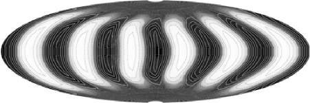
Figure 1: The radial velocity in the magnetoconvection case with 6-fold azimuthal symmetry at $r=0.59\,r_{0}$, normalized with its maximum given by $V_{r}=16.98\,\eta/D$. In the grey scale coding, white and black correspond to $-1$ and $+1$, that is, downflows and upflows, respectively, and the contour lines to $\pm 0.1,\,\pm 0.3,\,\pm 0.5,\,\pm 0.7,\,\pm 0.9$.

The first example considered is adopted from Olson et al. (1999) with the governing parameters $\mbox{{E}}=3\times 10^{-4}$, $\mbox{{Ra}}=94(=1.5\mbox{{Ra}}_{c}$, where $\mbox{{Ra}}_{c}$ means the critical value of Ra) and $\mbox{{Pr}}=\mbox{{Pm}}=1$. Moreover, an axisymmetric toroidal magnetic field is imposed via an inhomogeneous boundary condition of the form

$$B_{\varphi}=B_{0}\sin(2\vartheta)\quad\mbox{at}\enspace r=r_{i},\,\,\,\,\,r=r_{0}\,.$$ (27)

Figure 1 shows the radial velocity field at $r=0.59\,r_{0}$ for an Elsasser number of the imposed field $\Lambda_{0}=1$, where $\Lambda_{0}$ is defined according to (6) but with $B$ replaced by $B_{0}$. A typical columnar convection pattern is revealed. Apart from a steady azimuthal drift of the convection columns the flow and also the magnetic field are steady. In addition, the azimuthal drift and so the remaining time dependence can be removed by a transformation to a corotating frame of reference. The electromotive force $\boldsymbol{\mathcal{E}}$ is identical in both the original and the corotating frame (e.g., Rädler and Stepanov, 2006).

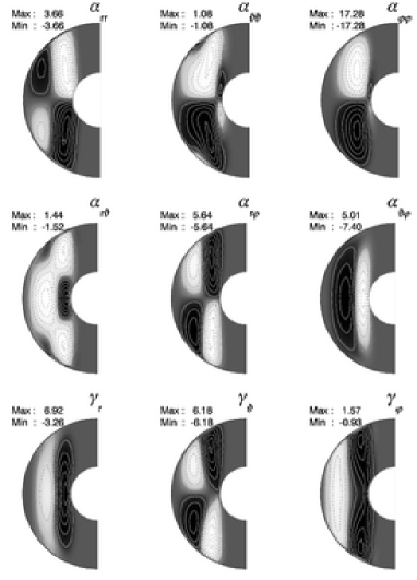
Figure 2: Components of the symmetric $\boldsymbol{\alpha}$-tensor and the $\boldsymbol{\gamma}$-vector in a meridional plane in the magnetoconvection example, determined by method I, in units of $\eta/D$. For each component the grey scale (white – negative, black – positive values) is separately adjusted to its maximum modulus. Note the negative signs in the definitions of $\boldsymbol{\alpha}$ and $\boldsymbol{\gamma}$ in equation (14).

The magnetic Reynolds number Rm is about 12, that is too low for the onset of self-sustaining dynamo action. Nevertheless, fundamental effects of the convection, which are of high interest for a dynamo, can be analysed in terms of mean fields, for example the generation of a poloidal from a toroidal field. The ratio of magnetic to kinetic energy density is about 10, and the resulting field strength is described by $\Lambda\approx 0.6$.

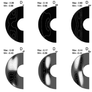
Figure 3: The symmetric diffusivity tensor $\mathbf{D}$ in the meridional plane in the magnetoconvection example, determined by method I, in units of $\eta$. Grey scales as in figure 2.

Figure 2 shows the six independent components of the tensor $\boldsymbol{\alpha}$ and the three components of the vector $\boldsymbol{\gamma}$ in a meridional plane derived by approach I. All mean-field coefficients are essentially determined by the columnar convection outside the inner core tangent cylinder. As a consequence of the symmetry properties of the velocity field and the induction equation, all mean-field coefficients are either symmetric or antisymmetric with respect to the equatorial plane. The diagonal components of $\boldsymbol{\alpha}$, for instance, are antisymmetric, in its major contributions negative in the northern and positive in the southern hemisphere. Among the $\boldsymbol{\alpha}$-components, $\alpha_{\varphi\varphi}$ dominates, indicating that the generation of a poloidal field from a toroidal one is more effective than the reversed process. However, due to the other non-vanishing components, especially $\alpha_{rr}$, $\alpha_{r\vartheta}$ and $\alpha_{\vartheta\vartheta}$, generation of toroidal field by an $\alpha$-effect also takes place.

The mean-field diffusivity tensor $\mathbf{D}$ is given by

$$D_{\kappa\lambda}=\eta\delta_{\kappa\lambda}+\beta_{\kappa\lambda}\,.$$ (28)

Its components are shown in figure 3. Although the molecular magnetic diffusivity is rather high ($\mbox{{Pm}}=1$) and the vigour of the convection is rather low ($\mbox{{Ra}}=1.5\mbox{{Ra}}_{c}$), the turbulent diffusion is of the same order as the molecular one in the convection region.

The diffusivity tensor $\mathbf{D}$ has the interesting property of being positive definite everywhere. This can be concluded from the fact that all its diagonal elements as well as all sub-determinants are positive. As explained in appendix B, this property implies that the induction effects expressed by $\mathbf{D}$ do not contribute to a growth of the total magnetic energy stored in the mean magnetic field but favour its dissipation. Because the fact that $\beta_{\kappa\lambda}$ has been defined with some arbitrariness, this statement has, however, to be considered with some caution (see also appendix B).

The $\boldsymbol{\delta}$-vector and the $\boldsymbol{\kappa}$-tensor (which are not displayed here) have been derived as well, and they are used in the magnetoconvection and dynamo calculations of section 6.

Figure 4: $(\alpha_{\varphi\varphi})_{\mathrm{rms}}$ in units of $\eta/D$ (left), the ratio $(\alpha_{r\varphi})_{\mathrm{rms}}/(\alpha_{\varphi\varphi})_{\mathrm{rms}}$ (middle), and the diagonal components of $(\beta_{\kappa\lambda})_{\mathrm{rms}}$ in units of $\eta$ (right) in the magnetoconvection case, in dependence on the Elsasser number $\Lambda$.

5.2 Quenching of mean-field coefficients

We point out that the velocity $\mathbf{v}$ needed for the determination of the mean-field coefficients $\tilde{a}_{\kappa\lambda}$, $\tilde{b}_{\kappa\lambda r}$ and $\tilde{b}_{\kappa\lambda\vartheta}$ were taken from simulations with non-zero mean magnetic field $\mathbf{\overline{B}}$. Therefore, the resulting coefficients are already subject to a magnetic quenching corresponding to this magnetic field. In this respect, results obtained with various $\mathbf{\overline{B}}$, measured by the Elsasser number $\Lambda$, are of interest. Figure 4 (left) shows $(\alpha_{\varphi\varphi})_{\mathrm{rms}}$, the r.m.s. value of $\alpha_{\varphi\varphi}$, as a function of $\Lambda$. The increase of this quantity in the presence of a weak magnetic field, that is for small $\Lambda$, is due to an increasing vigor of convection by the relaxation of the geostrophic constraint (Fearn, 1998). A strong magnetic field however inhibits convection and reduces $(\alpha_{\varphi\varphi})_{\mathrm{rms}}$. The kinetic energy of the convection varies with $\Lambda$ similar to $(\alpha_{\varphi\varphi})_{\mathrm{rms}}$. The other $\boldsymbol{\alpha}$ components are also quenched. The quenching is however not the same for different components, leading to varying amplitude relations among these components for varying strength of the mean magnetic field (figure 4 middle). In addition to the $\boldsymbol{\alpha}$-quenching, e.g., also a $\boldsymbol{\beta}$-quenching takes place (figure 4 right).

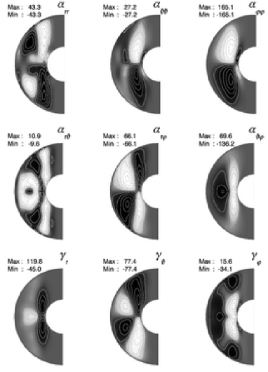
Figure 5: Components of the symmetric $\boldsymbol{\alpha}$-tensor and the $\boldsymbol{\gamma}$-vector in a meridional plane in the geodynamo example, determined by method I, in units of $\eta/D$. Grey scales as in figure 2.

5.3 A quasi-steady geodynamo

As a further example a quasi-steady geodynamo model is examined, which has been used before as a numerical dynamo benchmark (Christensen et al., 2001). The governing parameters have been chosen to be $\mbox{{E}}=10^{-3}$, $\mbox{{Ra}}=100\,(=1.79\mbox{{Ra}}_{c})$, $\mbox{{Pr}}=1$ and $\mbox{{Pm}}=5$. The columnar convection pattern is similar to that in the magnetoconvection example (figure 1), but with a natural 4-fold azimuthal symmetry. The intensity of the fluid motion is characterised by $\mbox{{Rm}}\approx 40$, and the magnetic energy density exceeds the kinetic one by a factor of 20. Again, except for an azimuthal drift of the convection columns, the velocity field is stationary.

The components of the $\boldsymbol{\alpha}$-tensor and the $\boldsymbol{\gamma}$-vector are shown in figure 5. Among the $\boldsymbol{\alpha}$-components, $\alpha_{\varphi\varphi}$ again dominates, indicating a very efficient generation of poloidal from toroidal magnetic field. The components $\alpha_{rr}$, $\alpha_{r\vartheta}$ and $\alpha_{\vartheta\vartheta}$ are somewhat lower in amplitude. Since the influence of the differential rotation on the generation of toroidal field is negligible, this example can be classified as an $\alpha^{2}$-dynamo. The imbalance in the amplitudes of the $\alpha$-components is reflected in the larger strength of the mean poloidal field compared to the mean toroidal field. As before in the example of magnetoconvection, the $\boldsymbol{\gamma}$-effect acts to expel flux from the central dynamo region where the convection takes place.

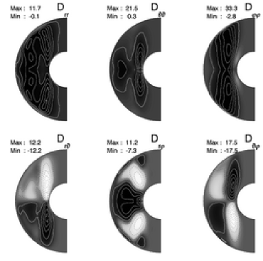
Figure 6: Components of the symmetric diffusivity tensor $\mathbf{D}$ in a meridional plane in the geodynamo example, determined by method I, in units of $\eta$. Grey scales as in figure 2.

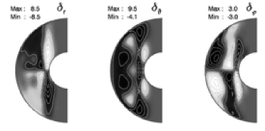
Figure 7: Components of the $\boldsymbol{\delta}$-vector in a meridional plane in the geodynamo example, determined by method I, in units of $\eta$. Grey scales as in figure 2.

The corresponding diffusivity tensor $\mathbf{D}$ is displayed in figure 6. The turbulent diffusivity $\boldsymbol{\beta}$ exceeds the molecular one, $\eta$, by more than a factor of 10 in the convection region outside the inner core tangent cylinder, leading to a very efficient diffusion of the mean magnetic field.

There is a weak negative contribution to $D_{\varphi\varphi}$ at the inner boundary close to the equator, which is negligible in the mean-field model of section 6.3. The diffusivity tensor $\mathbf{D}$ thus slightly deviates from being positive definite. We argue in appendix B that another than our particular choice $\mathsfi{b}_{\kappa\lambda\varphi}=0$ will lead to another $\mathbf{D}$ without changing $\boldsymbol{\mathcal{E}}$ and thus the physical situation. Furthermore, a parametrisation of $\boldsymbol{\mathcal{E}}$ considering higher than first-order derivatives of $\mathbf{\overline{B}}$ will also lead to changes of the low-order mean-field coefficients. In section 6.4 we will see the need of a better parametrisation of $\boldsymbol{\mathcal{E}}$ in the geodynamo case.

As for the $\delta$-effect we recall that the combination of this effect with a mean rotational shear may constitute a dynamo (Rädler, 1969, 1970, 1986; Roberts, 1972; Rädler et al., 2003). A dynamo mechanism of that kind, however, can not play a dominant role here, since neither $\mathbf{\overline{V}}$ nor $\boldsymbol{\gamma}$ imply a sufficiently strong shear. As we will see in section 6.5 below, however, the $\boldsymbol{\delta}$ terms, which are displayed in figure 7, may diminish the decay of a mean magnetic field.

5.4 Limitation of SOCA

The mean-field coefficients determined by approach I and approach II (SOCA) show for all Rm an almost perfect congruence of their profiles. However, mean-field coefficients determined by means of SOCA exhibit typically overestimated amplitudes for $\mbox{{Rm}}\gtrsim 10$.

Figure 8: The quantity $(\alpha_{\varphi\varphi})_{\mathrm{rms}}$ in the geodynamo case, in units of $\eta/D$, with $\alpha_{\varphi\varphi}$ determined by methods I and II (solid and dashed line, respectively) in dependence on Rm.

In figure 8, $(\alpha_{\varphi\varphi})_{\mathrm{rms}}$ is plotted versus Rm. In all calculations from which the mean-field coefficients were derived, $v$ was the same, and the variation of Rm is only due to a variation of $\eta$ or Pm which, for the calculation of $\mathbf{b}$ in equations (19) or (21), can be chosen differently from their values in the original model simulations. For small Rm the results of approaches I and II coincide and vary linearly with Rm. For $\mbox{{Rm}}\gtrsim 10$, the slope of $(\alpha_{\varphi\varphi})_{\mathrm{rms}}$ determined by approach I flattens. In particular, $\alpha_{\varphi\varphi}$ derived by approach I, that is, without restriction to SOCA, leads to amplitudes which are, e.g., for $\mbox{{Rm}}=40$ about $30\%$ smaller than those gained by approach II, that is, with SOCA calculations. The consequences for the dynamo action in a mean-field model are studied in the following section.

Let us add some explanation for the linear dependence of $(\alpha_{\varphi\varphi})_{\mathrm{rms}}$ on Rm observed in both approaches for small Rm, and in approach II for all Rm. In SOCA, when assuming a steady velocity $\mathbf{v}$, an $\boldsymbol{\alpha}$-component like $\alpha_{\varphi\varphi}$, say simply $\alpha$, is given by $\alpha=fv^{2}D/\eta$, where $f$ is a purely numerical factor. We may write this also in the forms $\alpha=(f\eta/D)\mbox{{Rm}}^{2}$ or $\alpha=fv\mbox{{Rm}}$. If $\eta$ and $D$ are fixed, $\alpha$ appears to be proportional to $\mbox{{Rm}}^{2}$, which may then vary with $v$. If, however, $v$ is fixed, $\alpha$ proves to be proportional to Rm, which may vary with $\eta$. This corresponds to the results presented in figure 8. The deviation of the results for $(\alpha_{\varphi\varphi})_{\mathrm{rms}}$ obtained in approach I from the linearity in Rm indicates that we are no longer in the range of applicability of SOCA or that the time variation of $\mathbf{v}$ is no longer sufficiently weak.

The usually given sufficient condition for the applicability of SOCA in the limit of steady motions reads $\mbox{{Rm}}\ll 1$, where Rm is defined with a typical length of the fluid flow. Even if this length is slightly overestimated by $D$ used in our definition of Rm, our finding of the applicability of SOCA for $\mbox{{Rm}}\lesssim 10$ is very remarkable.

6 Comparison between numerical simulations and mean-field models

6.1 Mean-field model

In order to compare direct numerical simulations and mean-field theory, an axisymmetric mean-field dynamo model involving all 27 mean-field coefficients $\tilde{a}_{\kappa\lambda}$, $\tilde{b}_{\kappa\lambda r}$, and $\tilde{b}_{\kappa\lambda\vartheta}$ has been constructed. The model also enables isolating certain dynamo processes.

Decomposing the axisymmetric mean magnetic field $\mathbf{\overline{B}}$ in its poloidal and toroidal parts,

$$\mathbf{\overline{B}}=\mathbf{\overline{B}}_{\mathrm{pol}}+\mathbf{\overline{B}}_{\mathrm{tor}}$$ (29)

with

$$\mathbf{\overline{B}}_{\mathrm{pol}}=\boldsymbol{\nabla}\times A\mathbf{e}_{\varphi}\,,\quad\mathbf{\overline{B}}_{\mathrm{tor}}=B\mathbf{e}_{\varphi},$$ (30)

where $\mathbf{e}_{\varphi}$ is the unit vector in azimuthal direction, we may write the induction equation (7) as

$$\frac{\partial A}{\partial t} = \frac{1}{r\sin\vartheta}\overline{\mathbf{V}}_{\mathrm{pol}}\cdot\boldsymbol{\nabla}(r\sin\vartheta A)+\mathcal{E}_{\varphi}-\eta\Delta^{\prime}A$$ (31)

$$\frac{\partial B}{\partial t} = r\sin\vartheta\,\overline{\mathbf{V}}_{\mathrm{pol}}\cdot\boldsymbol{\nabla}\left(\frac{B}{r\sin\vartheta}\right)+\frac{1}{r}\frac{\partial({\overline{V}}_{\varphi}/r\sin\vartheta,\,r\sin\vartheta A)}{\partial(r,\vartheta)}+(\boldsymbol{\nabla}\times\boldsymbol{\mathcal{E}}_{\mathrm{pol}})_{\varphi}-\eta\Delta^{\prime}B\,,$$ (32)

where $\Delta^{\prime}=\Delta-1/(r\sin\vartheta)^{2}$. Here, the notations $\boldsymbol{\mathcal{E}}_{\mathrm{pol}}=(\mathcal{E}_{r},\mathcal{E}_{\vartheta},0)$ and $\overline{\mathbf{V}}_{\mathrm{pol}}=(\overline{V}_{r},\overline{V}_{\vartheta},0)$ have been used. $\boldsymbol{\mathcal{E}}$ in its dependence on $\mathbf{\overline{B}}$ has to be taken from (11). The above equations are then solved in a spherical shell with electrically insulating inner and outer surroundings. Thus, the mean magnetic field is assumed to continue as a potential field in both parts exterior to the fluid shell.

The two coupled equations (31)-(32) are solved by a finite difference method on an equidistant grid in radial and latitudinal direction. An alternating direction implicit scheme for parabolic equations with mixed derivatives according to McKee et al. (1996) has been used to discretise the equations. This enables an efficient implicit treatment of advection and diffusion terms, whereas mixed and higher order derivatives are treated explicitly.

6.2 Magnetoconvection

How well do the results given by mean-field models match with the corresponding azimuthally averaged fields determined by direct numerical simulations? Let us first consider the rotating magnetoconvection model discussed in section 5.1. Figure 9 presents a comparison between direct numerical simulations and mean-field calculations. In the first row, the azimuthally averaged magnetic field components resulting from the direct numerical simulation are shown. They correspond in great detail to the results of our mean-field model (second row), in which all 27 mean-field coefficients have been used. The poloidal field is dipolar with inverse flux spots near the equatorial plane, and the applied azimuthal field is expelled from the region occupied by the convection columns.

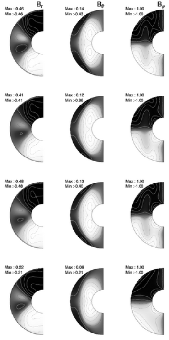
Figure 9: Comparison between numerical simulations and mean-field calculations in the example of magnetoconvection: azimuthally averaged magnetic field components resulting from a direct numerical simulation (first row), results given by the mean-field model based on all 27 coefficients derived by approach I (second row), mean-field calculation with coefficients derived applying SOCA (approach I with $\mathbf{G}=\mathbf{0}$, third row), and mean-field calculation with coefficients for isotropic turbulence (last row). Maxima and minima of the field components are given in units of $(\varrho\mu\eta\Omega)^{1/2}$. Grey scales as in figure 2.

A mean-field simulation relying on mean-field coefficients derived in SOCA (third row in figure 9) fits equally well. This reflects that mean-field coefficients given by SOCA, even overestimated by a few per cent in their amplitudes though, still lead to a reliable parametrisation of the mean electromotive force in this parameter regime. Moreover, amplitude deviations simultaneous in $\boldsymbol{\alpha}$ and $\boldsymbol{\beta}$ might not strongly influence the efficiency of the generation of poloidal from toroidal magnetic field and vice versa, as suggested by a simple scaling analysis: The efficiency of these processes can be expressed by the dimensionless number $P=\alpha_{0}^{2}\,D^{2}/\beta_{0}^{2}$. Here, $\alpha_{0}$ and $\beta_{0}$ mean typical values for the $\alpha$-effect and the turbulent diffusivity, respectively, and $D$ stands for a typical length scale. Since $\boldsymbol{\alpha}$ and $\boldsymbol{\beta}$ are likewise overestimated in their amplitudes, this factor cancels out and has no influence on $P$. As a consequence, the resulting field resembles the mean field displayed in the second row, even though the applied mean-field coefficients have larger amplitudes.

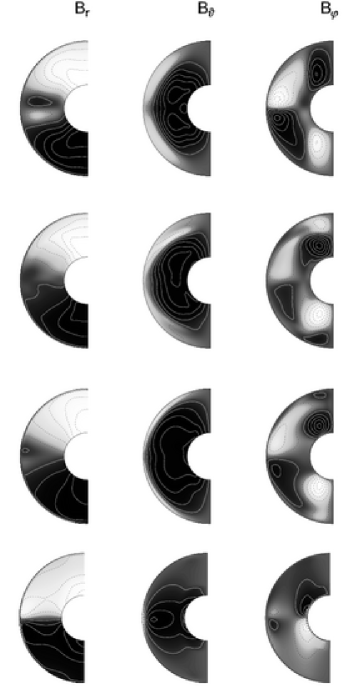
Figure 10: Comparison between numerical simulations and mean-field calculations in the example of the geodynamo: azimuthally averaged magnetic field components resulting from a direct numerical simulation (first row), results as given by mean-field modelling with coefficients derived by approach I (second row), mean-field calculation with coefficients in SOCA (approach I with $\mathbf{G}=\mathbf{0}$, third row), and with coefficients for isotropic turbulence (last row). Different from the solution of the direct numerical calculation which is stationary, all mean-field solutions decay exponentially with decay rates $\lambda=3.5\,\eta/D^{2}$ (second row), $\lambda=6.5\,\eta/D^{2}$ (third row), and $\lambda\approx 75\,\eta/D^{2}$ (last row).

The mean field components shown in the last row of figure 9 have been determined applying the isotropic approximation $\alpha_{\lambda\kappa}=\alpha_{I}\delta_{\lambda\kappa}$, $\beta_{\lambda\kappa}=\beta_{I}\delta_{\lambda\kappa}$. Concerning the coefficients $\alpha_{I}$ and $\beta_{I}$ we rely on SOCA results for isotropic turbulence in the limit of steady motion (see, e.g., Krause and Rädler (1980) or Rädler (2000)) and put

$$\alpha_{I}=-\frac{1}{3\eta}\overline{\mathbf{a}\cdot(\boldsymbol{\nabla}\times\mathbf{a})}\quad\mathrm{and}\quad\beta_{I}=\frac{1}{3\eta}\overline{\mathbf{a}^{2}}\,,$$ (33)

where $\mathbf{a}$ is the vector potential of $\mathbf{v}$ specified by $\boldsymbol{\nabla}\cdot\mathbf{a}=0$. With this choice of the mean-field coefficients the profile of the toroidal field clearly deviates from that in the cases considered before. It is less diffused at midlatitudes and mid radii where convection takes place. This difference can be attributed to the absence of the $\gamma$-effect. Already in this simple example the isotropic approximation fails to reproduce the axisymmetric field in satisfactory agreement with corresponding numerical simulations. This indicates that in general more mean-field coefficients must be taken into account in order to grasp all relevant dynamo effects. In addition there are deviations of about 50% in the amplitudes of the poloidal field.

6.3 Geodynamo

Consider now again the geodynamo model of section 5.3. In figure 10 the azimuthally averaged field components resulting from the numerical simulation are shown in comparison with results given by mean-field modelling. Figure 10 is organised in the same way as figure 9 before. That is, azimuthally averaged field components resulting from a direct numerical simulation have been plotted in the first row, the second row shows results obtained by corresponding mean-field calculations, the third row contributes results obtained by mean-field modelling with the coefficients determined in SOCA, while for the results presented in the last row, the isotropic approximation (33) has been applied. Note that only the direct numerical simulation results in a steady dynamo. All mean-field models shown in comparison are subcritical and the magnetic fields decay according to $\mathbf{\overline{B}}=\mathbf{\overline{B}}_{0}\exp(-\lambda t)$, where $\mathbf{\overline{B}}_{0}$ denotes the field configuration reached after an initial transition phase, and the decay rate $\lambda$ is positive in these examples. Therefore, decay rates rather than amplitudes are compared.

As in the previous example, both mean-field models relying on all 27 mean-field coefficients (second and third row in figure 10) correspond best to the direct numerical simulation and succeed in reproducing all essential features of the field given in the first row. However, both mean-field models are slightly subcritical with $\lambda=3.5\,\eta/D^{2}$ and $\lambda=6.5\,\eta/D^{2}$, respectively, which comes along with topological differences in $\overline{B}_{\varphi}$. The flux bundles at low latitudes near the outer boundary are more strongly diffused in the mean-field models. The high diffusion in this region is due to the strong $\gamma$-effect, which leads to an advection of oppositely oriented mean toroidal fields towards the equator, resulting in large gradients.

Although SOCA is, strictly speaking, not justified anymore, the resulting mean field components in the third row are remarkably similar to those obtained by mean-field modelling without applying SOCA (second row). For an explanation we refer again to the scaling argument given above in the context of the magnetoconvection example.

Again, mean-field coefficients in the isotropic approximation do not lead to reliable results anymore, as can be seen from the last row in figure 10. There are not only differences in the field distribution, but also the decay rate, $\lambda\approx 75\,\eta/D^{2}$, is drastically high.

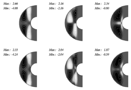
Figure 11: Comparison between electromotive forces in the magnetoconvection example. First row: $\mathcal{E}^{\mathrm{DNS}}_{r},\mathcal{E}^{\mathrm{DNS}}_{\vartheta},\mathcal{E}^{\mathrm{DNS}}_{\varphi}$, second row: $\mathcal{E}^{\mathrm{MF1}}_{r},\mathcal{E}^{\mathrm{MF1}}_{\vartheta},\mathcal{E}^{\mathrm{MF1}}_{\varphi}$. Maxima and minima are given in units of $(\eta/D)\,(\varrho\mu\eta\Omega)^{1/2}$.

6.4 Limits of the representation of the mean electromotive force

The difficulties of mean-field models in accurately reproducing mean magnetic fields compared to direct numerical simulations, which arise in the example of the geodynamo model, are due to an inadequate parametrisation of $\boldsymbol{\mathcal{E}}$. Let us compare $\boldsymbol{\mathcal{E}}^{\mathrm{DNS}}$, that is $\boldsymbol{\mathcal{E}}$ as immediately extracted from the direct numerical simulation, with $\boldsymbol{\mathcal{E}}^{\mathrm{MF1}}$ defined by $\mathcal{E}^{\mathrm{MF1}}_{\kappa}=\tilde{a}_{\kappa\lambda}\overline{B}_{\lambda}+\tilde{b}_{\kappa\lambda r}\,\partial\overline{B}_{\lambda}/\partial r+1/r\,\tilde{b}_{\kappa\lambda\vartheta}\,\partial\overline{B}_{\lambda}/\partial\vartheta$. For the computation of $\boldsymbol{\mathcal{E}}^{\mathrm{MF1}}$, both $\mathbf{\overline{B}}$ and its gradient have also been taken from the direct numerical simulation. We further define the quantity

$$\delta\mathcal{E}=\frac{<|\boldsymbol{\mathcal{E}}^{\mathrm{DNS}}-\boldsymbol{\mathcal{E}}^{\mathrm{MF1}}|>}{<|\boldsymbol{\mathcal{E}}^{\mathrm{DNS}}|>}$$ (34)

where $<\cdots>$ means spatial averaging.

Consider first the magnetoconvection example. Figure 11 shows that $\boldsymbol{\mathcal{E}}^{\mathrm{DNS}}$ and $\boldsymbol{\mathcal{E}}^{\mathrm{MF1}}$ are in reasonable agreement. We find $\delta\mathcal{E}\approx 0.28$. Therefore, a parametrisation of $\boldsymbol{\mathcal{E}}$ considering no higher than first-order derivatives of $\mathbf{\overline{B}}$ is adequate in this example.

In contrast, this is no longer true for the geodynamo model. In this case $\delta\mathcal{E}>4$ has been found, indicating that a parametrisation according to (11) no longer describes the actual $\boldsymbol{\mathcal{E}}$ reasonably well. The assumption of a sufficiently weak spatial variation of $\mathbf{\overline{B}}$, which is needed to truncate the series expansion of $\boldsymbol{\mathcal{E}}$ in (11), breaks down. In fact, higher order derivatives of $\mathbf{\overline{B}}$ become large and spoil the representation (11) of $\boldsymbol{\mathcal{E}}$ in a rather uncontrolled manner.

This finding is consistent with the following observations. The power spectrum of the radially averaged mean magnetic field in the example of the geodynamo model exhibits a peak at $l=4$ containing 15% of the total power. In contrast, the corresponding spectrum in the magnetoconvection example does not possess noticeable contributions for $l>2$, suggesting that the mean-field is indeed smoother in this example. Furthermore, the magnetoconvection simulation has been repeated with more complicated imposed toroidal fields in order to trigger steeper gradients in the mean field. In this way, it is indeed possible to destroy the close match between $\boldsymbol{\mathcal{E}}^{\mathrm{DNS}}$ and $\boldsymbol{\mathcal{E}}^{\mathrm{MF1}}$ as seen in figure 11.

6.5 Significance of mean-field coefficients

In order to investigate the significance of the various mean-field coefficients we carried out a number of test calculations with different sets of mean-field coefficients for the geodynamo case. As already presented in section 6.3, the inclusion of all $\tilde{a}_{\kappa\lambda}$ and $\tilde{b}_{\kappa\lambda\nu}$ leads to the decay rate of $\lambda=3.5\,\eta/D^{2}$.

In one series of calculations we only used the $\tilde{a}_{\kappa\lambda}$ and disregarded the $\tilde{b}_{\kappa\lambda\nu}$, increased however the molecular diffusivity to $\mbox{{Pm}}=1$. With all $\tilde{a}_{\kappa\lambda}$ the decay rate of the dominant dipolar mode is $\lambda=2.1\,\eta/D^{2}$. Using only the diagonal $\tilde{a}_{\kappa\kappa}$ results in $\lambda=-4.8\,\eta/D^{2}$. Besides the diagonal terms, $\tilde{a}_{r\varphi}$ and $\tilde{a}_{\vartheta\varphi}$ are most important. They provide a strong $\gamma$-effect, which as already stated above, acts to expel flux from the central dynamo region and results in a decay with $\lambda=4.9\,\eta/D^{2}$. As seen in section 6.3 by comparing with the numerical simulations, the $\gamma$-effect is crucial for the geodynamo. Furthermore it leads to a preference of dipolar modes compared to quadrupolar modes, that is, modes being antisymmetric or symmetric, respectively, about the equatorial plane.

With all $\tilde{a}_{\kappa\lambda}$ coefficients included, we next studied the influence of the $\tilde{b}_{\kappa\lambda\nu}$ coefficients, now again for a molecular diffusivity described by $\mbox{{Pm}}=5$. With the diagonal terms only, diffusion is significantly enhanced and the resulting dynamo solution is markedly subcritical with $\lambda=15\,\eta/D^{2}$. However, not all components of $\tilde{b}_{\kappa\lambda\nu}$ are conducive to the turbulent diffusion. If in addition all coefficients which contribute to the $\delta$-effect are considered the decay rate decreases to $\lambda=3.0\,\eta/D^{2}$ and the solution gets close to the case where all coefficients are included. This might be due to a constructive action of the combination of $\delta$-effect and some kind of mean shear occurring with $\mathbf{\overline{V}}$ or $\boldsymbol{\gamma}$, which, if stronger, could lead to a dynamo even in the absence of the $\alpha$-effect. As explained in appendix B, the $\delta$-effect has no direct influence on the energy stored in the mean magnetic field.

Altogether, the test calculations suggest a large set of mean-field coefficients to be considered in order to achieve reasonable agreement between mean-field models and numerical simulations. These are the $\boldsymbol{\alpha}$ and $\boldsymbol{\gamma}$ terms as well as the $\boldsymbol{\beta}$ and $\boldsymbol{\delta}$ terms. The $\boldsymbol{\kappa}$ terms, on the other hand, seem not to be of importance.

7 Conclusions

The knowledge of the mean-field coefficients is decisive in order to analyse and to model dynamo action in many astrophysical bodies. In this paper, two approaches to determine mean-field coefficients have been developed. While the numerical approach does not use intrinsic approximations, the analytical approach is based on the second-order correlation approximation.

The mean-field view is applied to two examples: a simulation of rotating magnetoconvection and of a quasi-stationary geodynamo. In both examples similar processes take place: the mutual generation of poloidal and toroidal magnetic fields by an $\alpha$-effect, flux expulsion from the dynamo region due to a $\gamma$-effect, and a strong turbulent diffusion, which might be moderated by a $\delta$-effect.

The calculation of mean-field coefficients provides insight into the reliability of frequently applied approximations in the framework of mean-field theory. Most dubious among them is the reduction of the $\alpha$-tensor to an isotropic tensor, which leaves dominating non-diagonal components unconsidered. A further, important simplification is the second-order correlation approximation. It typically leads to overestimated amplitudes of mean-field coefficients, whereas their profiles are rather unaffected.

The mean-field picture of geodynamo models is completed by the simulation of axisymmetric fields by means of a mean-field model, involving all mean-field coefficients determined. Test calculations with different sets of mean-field coefficients confirm their relation to the above mentioned dynamo processes. In addition, a comparison with azimuthally averaged fields resulting from direct numerical simulations reveals their significance. In the magnetoconvection and the geodynamo example considered here, the match between direct numerical simulations and mean-field simulations is good only if a large number of mean-field coefficients are involved which contribute to $\boldsymbol{\alpha}$, $\boldsymbol{\gamma}$, $\boldsymbol{\beta}$ and $\boldsymbol{\delta}$. The application of corresponding mean-field coefficients derived in the second-order correlation approximation leads to similar results.

The reliability of mean-field models relies on a proper parametrisation of $\boldsymbol{\mathcal{E}}$ in terms of the mean magnetic field. In the magnetoconvection example the traditional representation of the mean electromotive force considering no higher than first order derivatives of the mean magnetic field is valid. However, already in the geodynamo example it seems no longer to be justified and the assumption of scale separation is not fulfilled. This limits the applicability of some approximations commonly used within the mean-field theory. Nonetheless, even in the geodynamo example the spatial structure of the axisymmetric fields obtained by mean-field modelling corresponds roughly with that of the azimuthal averages extracted from the corresponding direct numerical simulation.

Appendix A Approach II – derivations and further results

We first determine $\mathbf{b}$ so that it satisfies equation (21) inside the fluid shell and continues as a potential field in its inner and outer surroundings. We represent $\mathbf{b}$ in the same form as $\mathbf{v}$ in (22) by writing

$$\mathbf{b}=-\boldsymbol{\nabla}\times(\mathbf{r}\times\boldsymbol{\nabla}\sigma)-\mathbf{r}\times\boldsymbol{\nabla}\tau$$ (35)

and expanding the scalars $\sigma$ and $\tau$ according to

$$\sigma=\sum_{l,m}\,\sigma_{l}^{m}(r)Y_{l}^{m}(\vartheta,\varphi)\,,\quad\tau=\sum_{l,m}\,\tau_{l}^{m}(r)Y_{l}^{m}(\vartheta,\varphi)\,,$$ (36)

where $\sigma_{l}^{m}(r)$ and $\tau_{l}^{m}(r)$ are complex functions satisfying $\sigma_{l}^{m*}=\sigma_{l}^{-m}$ and $\tau_{l}^{m*}=\tau_{l}^{-m}$, but $\sigma_{l}^{0}=\tau_{l}^{0}=0$, and $Y_{l}^{m}(\vartheta,\varphi)$ stands for spherical harmonics as explained above.

We note that (35) implies

$$L^{2}\sigma=-\mathbf{r}\cdot\mathbf{b}\,,\quad L^{2}\tau=-\mathbf{r}\cdot(\boldsymbol{\nabla}\times\mathbf{b})\,,$$ (37)

where

$$L^{2}f=\frac{1}{\sin\vartheta}\frac{\partial}{\partial\vartheta}\left(\sin\vartheta\,\frac{\partial f}{\partial\vartheta}\right)+\frac{1}{\sin^{2}\vartheta}\frac{\partial^{2}f}{\partial\varphi^{2}}\,.$$ (38)

Of course, if $\mathbf{b}$ in (35) is replaced, e.g., by $\nabla^{2}\mathbf{b}$, (37) applies with the same replacement. We further note that the $Y_{l}^{m}$ satisfy the eigenvalue equation

$$L^{2}Y_{l}^{m}+l(l+1)Y_{l}^{m}=0$$ (39)

and the orthogonality relation

$$\int Y_{l}^{m}(\vartheta,\varphi)\,Y_{l^{\prime}}^{m^{\prime}*}(\vartheta,\varphi)\,\mbox{d}\Omega=\frac{4\pi(l+|m|)!}{(2l+1)(l-|m|)!}\delta_{ll^{\prime}}\delta_{mm^{\prime}}\,,$$ (40)

where $\mbox{d}\Omega$ means $\sin\vartheta\,\mbox{d}\vartheta\,\mbox{d}\varphi$ and the integration is over all $\vartheta$ and $\varphi$ of the full solid angle. Here Ferrer’s normalization of the associated Legendre polynomials $P_{l}^{m}$ has been adopted.

Using these relations equation (21) can be reduced to

$$\frac{1}{r}\frac{\mbox{d}^{2}}{\mbox{d}r^{2}}\big{(}r\sigma^{m}_{l}\big{)}-\frac{l(l+1)}{r^{2}}\sigma^{m}_{l}=F^{m}_{l}\,,\quad\frac{1}{r}\frac{\mbox{d}^{2}}{\mbox{d}r^{2}}\big{(}r\tau^{m}_{l}\big{)}-\frac{l(l+1)}{r^{2}}\tau^{m}_{l}=G^{m}_{l}\,,$$ (41)

applying in the shell $r_{i}<r<r_{0}$, and

$$F^{m}_{l}=\frac{(2l+1)(l-|m|)!}{4\pi\eta l(l+1)(l+|m|)!}\int(\mathbf{v}\times\mathbf{\overline{B}})\cdot(\mathbf{r}\times\boldsymbol{\nabla}Y^{m*}_{l})\,\mbox{d}\Omega$$

$$G^{m}_{l}=\frac{(2l+1)(l-|m|)!}{4\pi\eta l(l+1)(l+|m|)!}\int(\boldsymbol{\nabla}\times(\mathbf{v}\times\mathbf{\overline{B}}))\cdot(\mathbf{r}\times\boldsymbol{\nabla}Y^{m*}_{l})\,\mbox{d}\Omega\,,$$ (42)

again with integrations over the full solid angle. The continuation of $\mathbf{b}$ as a potential field in the regions inside and outside the conducting shell requires

$$\frac{\mbox{d}\sigma^{m}_{l}}{\mbox{d}r}-\frac{l}{r}\sigma^{m}_{l}=\tau^{m}_{l}=0\quad\mbox{at}\quad r=r_{i}\,,\quad\frac{\mbox{d}\sigma^{m}_{l}}{\mbox{d}r}+\frac{l+1}{r}\sigma^{m}_{l}=\tau^{m}_{l}=0\quad\mbox{at}\quad r=r_{0}\,.$$ (43)

The solutions of (41) satisfying (43) can be written in the form

$$\sigma^{m}_{l}=-\int_{r_{i}}^{r_{0}}f_{l}(r,r^{\prime})F^{m}_{l}(r^{\prime}){r^{\prime}}^{2}\mbox{d}r^{\prime}\,,\quad\tau^{m}_{l}=-\int_{r_{i}}^{r_{0}}g_{l}(r,r^{\prime})G^{m}_{l}(r^{\prime}){r^{\prime}}^{2}\mbox{d}r^{\prime}$$ (44)

with Green’s functions $f_{l}$ and $g_{l}$ defined by

$$f_{l}(r,r^{\prime})=\frac{1}{(2l+1)r}\left\{\begin{array}[]{cl}\left(\displaystyle{\frac{r^{\prime}}{r}}\right)^{l}\,,&r^{\prime}\leq r\\ &\\ \left(\displaystyle{\frac{r}{r^{\prime}}}\right)^{l+1}\,,&r^{\prime}\geq r\end{array}\right.$$ (45)

and

$$g_{l}(r,r^{\prime})=\left\{\begin{array}[]{rl}\left(1-\left(\displaystyle{\frac{r_{i}}{r_{0}}}\right)^{2l+1}\right)^{-1}\,\left[f_{l}(r,r^{\prime})-\left(\displaystyle{\frac{r}{r_{0}}}\right)^{l}f_{l}(r_{0},r^{\prime})\right.\\ &\\ \left.-\left(\displaystyle{\frac{r_{i}}{r}}\right)^{l+1}f_{l}(r_{i},r^{\prime})+\displaystyle{\frac{r^{l}r_{i}^{l+1}}{r_{0}^{2l+1}}f_{l}(r_{i},r^{\prime})}\right],&r^{\prime}\leq r\\ &\\ \left(1-\left(\displaystyle{\frac{r}{r_{0}}}\right)^{2l+1}\right)^{-1}\,\left[f_{l}(r,r^{\prime})-\left(\displaystyle{\frac{r}{r_{0}}}\right)^{l}f_{l}(r_{0},r^{\prime})\right.\\ &\\ \left.-\left(\displaystyle{\frac{r_{i}}{r}}\right)^{l+1}f_{l}(r_{i},r^{\prime})+\displaystyle{\frac{r_{i}^{2l+1}}{r^{l+1}r_{0}^{l}}f_{l}(r_{0},r^{\prime})}\right],&r^{\prime}\geq r\,.\end{array}\right.$$ (46)

Indeed it becomes clear by inserting of (44) that (41) is satisfied. Since (45) and (46) imply

$$\frac{\partial f_{l}(r,r^{\prime})}{\partial r}-\frac{l}{r}f_{l}(r,r^{\prime}) = g_{l}(r,r^{\prime})=0\quad\mbox{at}\quad r=r_{i}$$

$$\frac{\partial f_{l}(r,r^{\prime})}{\partial r}+\frac{l+1}{r}f_{l}(r,r^{\prime}) = g_{l}(r,r^{\prime})=0\quad\mbox{at}\quad r=r_{0}\,,$$ (47)

(44) also satisfies (43).

Inserting now the representation of $\mathbf{v}$ as given by (22) and (23) into the relation for $F_{l}^{m}$ given by (42) and then the result for $F^{m}_{l}$ into the expression for $\sigma^{m}_{l}$ in (44), we arrive at

$$\sigma^{m}_{l}(r) = \frac{(2l+1)(l-|m|)!}{4\pi\eta l(l+1)(l+|m|)!}$$ (48)

$$\sum_{l^{\prime}}\int f_{l}(r,r^{\prime})\bigg{\{}\Big{[}{\hat{\phi}}^{m}_{l^{\prime}}(r^{\prime})R^{m}_{l^{\prime}l}(\vartheta^{\prime})$$

$$-\mbox{i}m\psi^{m}_{l^{\prime}}(r^{\prime})\Big{(}Q^{m}_{l^{\prime}l}(\vartheta^{\prime})+Q^{m}_{ll^{\prime}}(\vartheta^{\prime})\Big{)}\Big{/}\sin\vartheta^{\prime}\Big{]}{\overline{B}}_{r}(r^{\prime},\vartheta^{\prime})$$

$$-\frac{l^{\prime}(l^{\prime}+1)}{r^{\prime}}\phi^{m}_{l^{\prime}}(r^{\prime})Q^{m}_{l^{\prime}l}(\vartheta^{\prime}){\overline{B}}_{\vartheta}(r^{\prime},\vartheta^{\prime})$$

$$+\mbox{i}m\frac{l^{\prime}(l^{\prime}+1)}{r^{\prime}}\phi^{m}_{l^{\prime}}(r^{\prime})\Big{(}P^{m}_{l^{\prime}l}(\vartheta^{\prime})/\sin\vartheta^{\prime}\Big{)}{\overline{B}}_{\varphi}(r^{\prime},\vartheta^{\prime})\bigg{\}}\mbox{d}v^{\prime}\,.$$

The integration is over the whole fluid shell. When proceeding analogously with the relation for $G_{l}^{m}$ in (42), the result for $G^{m}_{l}$ contains derivatives of $\overline{B}_{r}$, $\overline{B}_{\vartheta}$, and $\overline{B}_{\varphi}$ with respect to $r$ and $\vartheta$. We may remove them by means of integration by parts. In this way we find

$$\tau^{m}_{l}(r) = \frac{(2l+1)(l-|m|)!}{4\pi\eta l(l+1)(l+|m|)!}\sum_{l^{\prime}}\int\bigg{\{}\tilde{g}_{l}(r,r^{\prime})$$ (49)

$$\times\Big{[}\mbox{i}m{\hat{\phi}}^{m}_{l^{\prime}}(r^{\prime})\Big{(}Q^{m}_{l^{\prime}l}(\vartheta^{\prime})+Q^{m}_{ll^{\prime}}(\vartheta^{\prime})\Big{)}\Big{/}\sin\vartheta^{\prime}-\psi^{m}_{l^{\prime}}(r^{\prime})R^{m}_{l^{\prime}l}(\vartheta^{\prime})\Big{]}{\overline{B}}_{r}(r^{\prime},\vartheta^{\prime})$$

$$-\frac{1}{r^{\prime}}\Big{[}l(l+1)g_{l}(r,r^{\prime})\Big{(}\mbox{i}m{\hat{\phi}}^{m}_{l^{\prime}}(r^{\prime})P^{m}_{l^{\prime}l}(\vartheta^{\prime})/\sin\vartheta^{\prime}-\psi^{m}_{l^{\prime}}(r^{\prime})Q^{m}_{ll^{\prime}}(\vartheta^{\prime})\Big{)}$$

$$+\mbox{i}ml^{\prime}(l^{\prime}+1)\tilde{g}_{l}(r,r^{\prime})\,\phi^{m}_{l^{\prime}}(r^{\prime})P^{m}_{l^{\prime}l}(\vartheta^{\prime})/\sin\vartheta^{\prime}\Big{]}{\overline{B}}_{\vartheta}(r^{\prime},\vartheta^{\prime})$$

$$+\frac{1}{r^{\prime}}\Big{[}l(l+1)g_{l}(r,r^{\prime})\Big{(}{\hat{\phi}}^{m}_{l^{\prime}}(r^{\prime})Q^{m}_{ll^{\prime}}(\vartheta^{\prime})+\mbox{i}m\psi^{m}_{l^{\prime}}(r^{\prime})P^{m}_{ll^{\prime}}(\vartheta^{\prime})/\sin\vartheta^{\prime}\Big{)}$$

$$-l^{\prime}(l^{\prime}+1)\tilde{g}_{l}(r,r^{\prime})\,\phi^{m}_{l^{\prime}}(r^{\prime})Q^{m}_{l^{\prime}l}(\vartheta^{\prime})\Big{]}{\overline{B}}_{\varphi}(r^{\prime},\vartheta^{\prime})\bigg{\}}\mbox{d}v^{\prime}$$

with $\tilde{g}_{l}(r,r^{\prime})=(1/r^{\prime})\,\partial\big{(}r^{\prime}g_{l}(r,r^{\prime})\big{)}/\partial r^{\prime}$.

The relations (35) and (36) together with (48) and (49) represent the wanted solution of the equation (21) for $\mathbf{b}$.

Let us now proceed to $\boldsymbol{\mathcal{E}}=\overline{\mathbf{v}\times\mathbf{b}}$. Expressing $\mathbf{v}$ according to (22) and (23) and $\mathbf{b}$ according to (35) and (36) we find

$${\mathcal{E}}_{r} = -2\sum_{l,l^{\prime}\,;\,m>0}\bigg{[}\mbox{Re}\Big{(}{\hat{\phi}}_{l^{\prime}}^{m*}\tau_{l}^{m}-\psi_{l^{\prime}}^{m*}{\hat{\sigma}}_{l}^{m}\Big{)}\,R^{m}_{l^{\prime}l}$$

$$+m\,\mbox{Im}\Big{(}{\hat{\phi}}_{l^{\prime}}^{m*}{\hat{\sigma}}_{l}^{m}+\psi_{l^{\prime}}^{m*}\tau_{l}^{m}\Big{)}\,\big{(}Q^{m}_{l^{\prime}l}+Q^{m}_{ll^{\prime}}\big{)}/\sin\vartheta\bigg{]}$$

$${\mathcal{E}}_{\vartheta} = +\frac{2}{r}\sum_{l,l^{\prime}\,;\,m>0}\bigg{[}l^{\prime}(l^{\prime}+1)\mbox{Re}\Big{(}\phi_{l^{\prime}}^{m*}\tau_{l}^{m}\Big{)}\,Q^{m}_{l^{\prime}l}-l(l+1)\mbox{Re}\Big{(}\psi_{l^{\prime}}^{m*}\sigma_{l}^{m}\Big{)}\,Q^{m}_{ll^{\prime}}$$ (50)

$$+m\,\bigg{(}l(l+1)\mbox{Im}\Big{(}{\hat{\phi}}_{l^{\prime}}^{m*}\sigma_{l}^{m}\Big{)}+l^{\prime}(l^{\prime}+1)\mbox{Im}\Big{(}\phi_{l^{\prime}}^{m*}{\hat{\sigma}}_{l}^{m}\Big{)}\bigg{)}\,P^{m}_{l^{\prime}l}/\sin\vartheta\bigg{]}$$

$${\mathcal{E}}_{\varphi} = -\frac{2}{r}\sum_{l,l^{\prime}\,;\,m>0}\bigg{[}l(l+1)\mbox{Re}\Big{(}{\hat{\phi}}_{l^{\prime}}^{m*}\sigma_{l}^{m}\Big{)}\,Q^{m}_{ll^{\prime}}-l^{\prime}(l^{\prime}+1)\mbox{Re}\Big{(}\phi_{l^{\prime}}^{m*}{\hat{\sigma}}_{l}^{m}\Big{)}\,Q^{m}_{l^{\prime}l}$$

$$+m\,\bigg{(}l^{\prime}(l^{\prime}+1)\mbox{Im}\Big{(}\phi_{l^{\prime}}^{m*}\tau_{l}^{m}\Big{)}+l(l+1)\mbox{Im}\Big{(}\psi_{l^{\prime}}^{m*}\sigma_{l}^{m}\Big{)}\bigg{)}\,P^{m}_{l^{\prime}l}/\sin\vartheta\bigg{]}\,.$$

The $\phi_{l}^{m}$, $\psi_{l}^{m}$, $\sigma_{l}^{m}$ and $\tau_{l}^{m}$ depend of course on $r$. The $P_{l^{\prime}l}^{m}$, $Q_{l^{\prime}l}^{m}$ and $R_{l^{\prime}l}^{m}$ are functions of $\vartheta$ defined by

$$P^{m}_{l^{\prime}l} = P^{|m|}_{l^{\prime}}(\cos\vartheta)P^{|m|}_{l}(\cos\vartheta)$$

$$Q^{m}_{l^{\prime}l} = P^{|m|}_{l^{\prime}}(\cos\vartheta)\frac{\mbox{d}P^{|m|}_{l}(\cos\vartheta)}{\mbox{d}\vartheta}$$ (51)

$$R^{m}_{l^{\prime}l} = \frac{\mbox{d}P^{|m|}_{l^{\prime}}(\cos\vartheta)}{\mbox{d}\vartheta}\frac{\mbox{d}P^{|m|}_{l}(\cos\vartheta)}{\mbox{d}\vartheta}+\frac{m^{2}}{\sin^{2}\vartheta}P^{|m|}_{l^{\prime}}(\cos\vartheta)P^{|m|}_{l}(\cos\vartheta)\,.$$

We may now insert the results (48) and (49) for $\sigma_{l}^{m}$ and $\tau_{l}^{m}$ into (50). Then the ${\mathcal{E}}_{\kappa}$ take indeed the form (24). Unfortunately the $K_{\kappa\lambda}$ are rather complex expressions. As an example we mention

$$K_{rr}(r,\vartheta;r^{\prime},\vartheta^{\prime}) = \frac{1}{2\pi\eta}\sum_{l,l^{\prime},l^{\prime\prime}\,;\ m>0}\frac{(2l+1)(l-|m|)!}{l(l+1)(l+|m|)!}$$ (52)

$$\times\Bigg{\{}\bigg{[}{\hat{f}}_{l}(r,r^{\prime})\,\mbox{Im}\Big{(}\psi^{m*}_{l^{\prime}}(r)\psi^{m}_{l^{\prime\prime}}(r^{\prime})\Big{)}+{\tilde{g}}_{l}(r,r^{\prime})\,\mbox{Im}\Big{(}{\hat{\phi}}^{m*}_{l^{\prime}}(r){\hat{\phi}}^{m}_{l^{\prime\prime}}(r^{\prime})\Big{)}\bigg{]}$$

$$\hskip 14.22636pt\times m\,R^{m}_{l^{\prime}l}(\vartheta)\,\Big{(}Q^{m}_{l^{\prime\prime}l}(\vartheta^{\prime})+Q^{m}_{ll^{\prime\prime}}(\vartheta^{\prime})\Big{)}\Big{/}\sin\vartheta^{\prime}\,$$

$$+\bigg{[}{\hat{f}}_{l}(r,r^{\prime})\,\mbox{Re}\Big{(}{\hat{\phi}}^{m*}_{l^{\prime}}(r)\psi^{m}_{l^{\prime\prime}}(r^{\prime})\Big{)}-{\tilde{g}}_{l}(r,r^{\prime})\,\mbox{Re}\Big{(}\psi^{m*}_{l^{\prime}}(r){\hat{\phi}}^{m}_{l^{\prime\prime}}(r^{\prime})\Big{)}\bigg{]}$$

$$\hskip 14.22636pt\times m^{2}\,\Big{(}Q^{m}_{l^{\prime}l}(\vartheta)+Q^{m}_{ll^{\prime}}(\vartheta)\Big{)}\,\Big{(}Q^{m}_{l^{\prime\prime}l}(\vartheta^{\prime})+Q^{m}_{ll^{\prime\prime}}(\vartheta^{\prime})\Big{)}\Big{/}(\sin\vartheta\sin\vartheta^{\prime})$$

$$+\bigg{[}{\hat{f}}_{l}(r,r^{\prime})\,\mbox{Re}\Big{(}\psi^{m*}_{l^{\prime}}(r){\hat{\phi}}^{m}_{l^{\prime\prime}}(r^{\prime})\Big{)}+{\tilde{g}}_{l}(r,r^{\prime})\,\mbox{Re}\Big{(}{\hat{\phi}}^{m*}_{l^{\prime}}(r)\psi^{m}_{l^{\prime\prime}}(r^{\prime})\Big{)}\bigg{]}$$

$$\hskip 14.22636pt\times R^{m}_{l^{\prime}l}(\vartheta)\,R^{m}_{l^{\prime\prime}l}(\vartheta^{\prime})$$

$$-\bigg{[}{\hat{f}}_{l}(r,r^{\prime})\,\mbox{Im}\Big{(}{\hat{\phi}}^{m*}_{l^{\prime}}(r){\hat{\phi}}^{m}_{l^{\prime\prime}}(r^{\prime})\Big{)}-{\tilde{g}}_{l}(r,r^{\prime})\,\mbox{Im}\Big{(}\psi^{m*}_{l^{\prime}}(r)\psi^{m}_{l^{\prime\prime}}(r^{\prime})\Big{)}\bigg{]}$$

$$\hskip 14.22636pt\times m\,\Big{(}Q^{m}_{l^{\prime}l}(\vartheta)+Q^{m}_{ll^{\prime}}(\vartheta)\Big{)}\,R^{m}_{l^{\prime\prime}l}(\vartheta^{\prime})/\sin\vartheta\Bigg{\}}$$

where $\hat{f}_{l}(r,r^{\prime})=(1/r)\,\partial\big{(}rf_{l}(r,r^{\prime})\big{)}/\partial r$.

Using now (25) and the orthogonality relations

$$\int_{0}^{\pi}P^{m}_{l^{\prime}l}(\vartheta)\sin\vartheta\mbox{d}\vartheta=\frac{2(l+|m|)!}{(2l+1)(l-|m|)!}\delta_{l^{\prime}l}$$

$$\int_{0}^{\pi}\big{(}Q^{m}_{l^{\prime}l}(\vartheta)+Q^{m}_{ll^{\prime}}(\vartheta)\big{)}\mbox{d}\vartheta=0$$ (53)

$$\int_{0}^{\pi}R^{m}_{l^{\prime}l}(\vartheta)\sin\vartheta\mbox{d}\vartheta=\frac{2l(l+1)(l+|m|)!}{(2l+1)(l-|m|)!}\delta_{l^{\prime}l}$$

we find $\tilde{a}_{rr}$ as given by (26).

In the same way all other $\tilde{a}_{\kappa\lambda}$ can be calculated. Unfortunately in the cases of $\tilde{a}_{\kappa\vartheta}$ and $\tilde{a}_{\kappa\varphi}$ the integration over $\vartheta$ can not be carried out with taking benefit of orthogonality relations like (53), and the need of numerical integrations remains. The results read

$$\tilde{a}_{\vartheta r}(r,\vartheta) = \frac{2}{\eta r}\sum_{l,l^{\prime}\,;\,m>0}\Bigg{\{}-l^{\prime}(l^{\prime}+1)\int_{r_{i}}^{r_{0}}\tilde{g}_{l}(r,r^{\prime})\mbox{Re}\Big{(}\phi^{m*}_{l^{\prime}}(r)\psi^{m}_{l}(r^{\prime})\Big{)}\,{r^{\prime}}^{2}\mbox{d}r^{\prime}\;Q^{m}_{l^{\prime}l}(\vartheta)$$ (54)

$$-\;l(l+1)\int_{r_{i}}^{r_{0}}f_{l}(r,r^{\prime})\mbox{Re}\Big{(}\psi^{m*}_{l^{\prime}}(r)\hat{\phi}^{m}_{l}(r^{\prime})\Big{)}\,{r^{\prime}}^{2}\mbox{d}r^{\prime}\;Q^{m}_{ll^{\prime}}(\vartheta)$$

$$+\;m\int_{r_{i}}^{r_{0}}\bigg{[}l^{\prime}(l^{\prime}+1)\hat{f}_{l}(r,r^{\prime})\mbox{Im}\Big{(}\phi^{m*}_{l^{\prime}}(r)\hat{\phi}^{m}_{l}(r^{\prime})\Big{)}$$

$$+l(l+1)f_{l}(r,r^{\prime})\mbox{Im}\Big{(}\hat{\phi}^{m*}_{l^{\prime}}(r)\hat{\phi}^{m}_{l}(r^{\prime})\Big{)}\bigg{]}\,{r^{\prime}}^{2}\mbox{d}r^{\prime}\;P^{m}_{l^{\prime}l}(\vartheta)/\sin\vartheta\Bigg{\}}$$

$$\tilde{a}_{\varphi r}(r,\vartheta) = \frac{2}{\eta r}\sum_{l,l^{\prime}\,;\,m>0}\Bigg{\{}\,l^{\prime}(l^{\prime}+1)\int_{r_{i}}^{r_{0}}\hat{f}_{l}(r,r^{\prime})\mbox{Re}\Big{(}\phi^{m*}_{l^{\prime}}(r)\hat{\phi}^{m}_{l}(r^{\prime})\Big{)}\,{r^{\prime}}^{2}\mbox{d}r^{\prime}\;Q^{m}_{l^{\prime}l}(\vartheta)$$ (55)

$$-\;l(l+1)\int_{r_{i}}^{r_{0}}f_{l}(r,r^{\prime})\mbox{Re}\Big{(}\hat{\phi}^{m*}_{l^{\prime}}(r)\hat{\phi}^{m}_{l}(r^{\prime})\Big{)}\,{r^{\prime}}^{2}\mbox{d}r^{\prime}\;Q^{m}_{ll^{\prime}}(\vartheta)$$

$$+\;m\int_{r_{i}}^{r_{0}}\bigg{[}l^{\prime}(l^{\prime}+1)\tilde{g}_{l}(r,r^{\prime})\mbox{Im}\Big{(}\phi^{m*}_{l^{\prime}}(r)\psi^{m}_{l}(r^{\prime})\Big{)}$$

$$-l(l+1)f_{l}(r,r^{\prime})\mbox{Im}\Big{(}\psi^{m*}_{l^{\prime}}(r)\hat{\phi}^{m}_{l}(r^{\prime})\Big{)}\bigg{]}\,{r^{\prime}}^{2}\mbox{d}r^{\prime}\;P^{m}_{l^{\prime}l}(\vartheta)/\sin\vartheta\Bigg{\}}$$

$$\tilde{a}_{r\vartheta}(r,\vartheta) = \frac{1}{\eta}\sum_{l,l^{\prime},l^{\prime\prime}\,;\,m>0}\frac{(2l+1)(l-|m|)!}{l(l+1)(l+|m|)!}$$ (56)

$$\times\Bigg{\{}R^{m}_{l^{\prime}l}(\vartheta)\Bigg{[}-m\int_{r_{i}}^{r_{0}}\bigg{\{}l(l+1)g_{l}(r,r^{\prime})\mbox{Im}\Big{(}\hat{\phi}^{m*}_{l^{\prime}}(r)\hat{\phi}^{m}_{l^{\prime\prime}}(r^{\prime})\Big{)}$$

$$+l^{\prime\prime}(l^{\prime\prime}+1)\tilde{g}_{l}(r,r^{\prime})\mbox{Im}\Big{(}\hat{\phi}^{m*}_{l^{\prime}}(r)\phi^{m}_{l^{\prime\prime}}(r^{\prime})\Big{)}\bigg{\}}\,r^{\prime}\mbox{d}r^{\prime}\int_{0}^{\pi}P^{m}_{l^{\prime\prime}l}(\vartheta^{\prime})\mbox{d}\vartheta^{\prime}$$

$$-l(l+1)\int_{r_{i}}^{r_{0}}g_{l}(r,r^{\prime})\mbox{Re}\Big{(}\hat{\phi}^{m*}_{l^{\prime}}(r)\psi^{m}_{l^{\prime\prime}}(r^{\prime})\Big{)}\,r^{\prime}\mbox{d}r^{\prime}\int_{0}^{\pi}Q^{m}_{ll^{\prime\prime}}(\vartheta^{\prime})\sin\vartheta^{\prime}\mbox{d}\vartheta^{\prime}$$

$$-l^{\prime\prime}(l^{\prime\prime}+1)\int_{r_{i}}^{r_{0}}\hat{f}_{l}(r,r^{\prime})\mbox{Re}\Big{(}\psi^{m*}_{l^{\prime}}(r)\phi^{m}_{l^{\prime\prime}}(r^{\prime})\Big{)}\,r^{\prime}\mbox{d}r^{\prime}\int_{0}^{\pi}Q^{m}_{l^{\prime\prime}l}(\vartheta^{\prime})\sin\vartheta^{\prime}\mbox{d}\vartheta^{\prime}\Bigg{]}$$

$$+m\Big{(}Q^{m}_{l^{\prime}l}(\vartheta)+Q^{m}_{ll^{\prime}}(\vartheta)\Big{)}\big{/}\sin\vartheta\Bigg{[}m\int_{r_{i}}^{r_{0}}\bigg{\{}l(l+1)g_{l}(r,r^{\prime})\mbox{Re}\Big{(}\psi^{m*}_{l^{\prime}}(r)\hat{\phi}^{m}_{l^{\prime\prime}}(r^{\prime})\Big{)}$$

$$+l^{\prime\prime}(l^{\prime\prime}+1)\tilde{g}_{l}(r,r^{\prime})\mbox{Re}\Big{(}\psi^{m*}_{l^{\prime}}(r)\phi^{m}_{l^{\prime\prime}}(r^{\prime})\Big{)}\bigg{\}}\,r^{\prime}\mbox{d}r^{\prime}\int_{0}^{\pi}P^{m}_{l^{\prime\prime}l}(\vartheta^{\prime})\mbox{d}\vartheta^{\prime}$$

$$-l(l+1)\int_{r_{i}}^{r_{0}}g_{l}(r,r^{\prime})\mbox{Im}\Big{(}\psi^{m*}_{l^{\prime}}(r)\psi^{m}_{l^{\prime\prime}}(r^{\prime})\Big{)}\,r^{\prime}\mbox{d}r^{\prime}\int_{0}^{\pi}Q^{m}_{ll^{\prime\prime}}(\vartheta^{\prime})\sin\vartheta^{\prime}\mbox{d}\vartheta^{\prime}$$

$$+l^{\prime\prime}(l^{\prime\prime}+1)\int_{r_{i}}^{r_{0}}\hat{f}_{l}(r,r^{\prime})\mbox{Im}\Big{(}\hat{\phi}^{m*}_{l^{\prime}}(r)\phi^{m}_{l^{\prime\prime}}(r^{\prime})\Big{)}\,r^{\prime}\mbox{d}r^{\prime}$$

$$\times\int_{0}^{\pi}Q^{m}_{l^{\prime\prime}l}(\vartheta^{\prime})\sin\vartheta^{\prime}\mbox{d}\vartheta^{\prime}\Bigg{]}\Bigg{\}}$$

$$\tilde{a}_{\vartheta\vartheta}(r,\vartheta) = \frac{1}{\eta r}\sum_{l,l^{\prime},l^{\prime\prime}\,;\,m>0}\frac{(2l+1)(l-|m|)!}{l(l+1)(l+|m|)!}$$ (57)

$$\times\Bigg{\{}\,l^{\prime}(l^{\prime}+1)Q^{m}_{l^{\prime}l}(\vartheta)\Bigg{[}m\int_{r_{i}}^{r_{0}}\bigg{\{}l(l+1)g_{l}(r,r^{\prime})\mbox{Im}\Big{(}\phi^{m*}_{l^{\prime}}(r)\hat{\phi}^{m}_{l^{\prime\prime}}(r^{\prime})\Big{)}$$

$$+\;l^{\prime\prime}(l^{\prime\prime}+1)\tilde{g}_{l}(r,r^{\prime})\mbox{Im}\Big{(}\phi^{m*}_{l^{\prime}}(r)\phi^{m}_{l^{\prime\prime}}(r^{\prime})\Big{)}\bigg{\}}\,r^{\prime}\mbox{d}r^{\prime}\int_{0}^{\pi}P^{m}_{l^{\prime\prime}l}(\vartheta^{\prime})\mbox{d}\vartheta^{\prime}$$

$$+\;l(l+1)\int_{r_{i}}^{r_{0}}g_{l}(r,r^{\prime})\mbox{Re}\Big{(}\phi^{m*}_{l^{\prime}}(r)\psi^{m}_{l^{\prime\prime}}(r^{\prime})\Big{)}\,r^{\prime}\mbox{d}r^{\prime}\int_{0}^{\pi}Q^{m}_{ll^{\prime\prime}}(\vartheta^{\prime})\sin\vartheta^{\prime}\mbox{d}\vartheta^{\prime}\Bigg{]}$$

$$-\;l^{\prime\prime}(l^{\prime\prime}+1)\int_{0}^{\pi}Q^{m}_{l^{\prime\prime}l}(\vartheta^{\prime})\sin\vartheta^{\prime}\mbox{d}\vartheta^{\prime}\Bigg{[}m\int_{r_{i}}^{r_{0}}\bigg{\{}l(l+1)f_{l}(r,r^{\prime})\mbox{Im}\Big{(}\hat{\phi}^{m*}_{l^{\prime}}(r)\phi^{m}_{l^{\prime\prime}}(r^{\prime})\Big{)}$$

$$+\;l^{\prime}(l^{\prime}+1)\hat{f}_{l}(r,r^{\prime})\mbox{Im}\Big{(}\phi^{m*}_{l^{\prime}}(r)\phi^{m}_{l^{\prime\prime}}(r^{\prime})\Big{)}\bigg{\}}\,r^{\prime}\mbox{d}r^{\prime}\;P^{m}_{l^{\prime}l}(\vartheta)/\sin\vartheta$$

$$-\;l(l+1)\int_{r_{i}}^{r_{0}}f_{l}(r,r^{\prime})\mbox{Re}\Big{(}\psi^{m*}_{l^{\prime}}(r)\phi^{m}_{l^{\prime\prime}}(r^{\prime})\Big{)}\,r^{\prime}\mbox{d}r^{\prime}\,Q^{m}_{ll^{\prime}}(\vartheta)\Bigg{]}\Bigg{\}}$$

$$\tilde{a}_{\varphi\vartheta}(r,\vartheta) = \frac{1}{\eta r}\sum_{l,l^{\prime},l^{\prime\prime}\,;\,m>0}\frac{(2l+1)(l-|m|)!}{l(l+1)(l+|m|)!}$$ (58)

$$\times\Bigg{\{}\,ml^{\prime}(l^{\prime}+1)P^{m}_{l^{\prime}l}(\vartheta)/\sin\vartheta\Bigg{[}m\int_{r_{i}}^{r_{0}}\bigg{\{}l(l+1)g_{l}(r,r^{\prime})\mbox{Re}\Big{(}\phi^{m*}_{l^{\prime}}(r)\hat{\phi}^{m}_{l^{\prime\prime}}(r^{\prime})\Big{)}$$

$$+\;l^{\prime\prime}(l^{\prime\prime}+1)\tilde{g}_{l}(r,r^{\prime})\mbox{Re}\Big{(}\phi^{m*}_{l^{\prime}}(r)\phi^{m}_{l^{\prime\prime}}(r^{\prime})\Big{)}\bigg{\}}\,r^{\prime}\mbox{d}r^{\prime}\int_{0}^{\pi}P^{m}_{l^{\prime\prime}l}(\vartheta^{\prime})\mbox{d}\vartheta^{\prime}$$

$$-\;l(l+1)\int_{r_{i}}^{r_{0}}g_{l}(r,r^{\prime})\mbox{Im}\Big{(}\phi^{m*}_{l^{\prime}}(r)\psi^{m}_{l^{\prime\prime}}(r^{\prime})\Big{)}\,r^{\prime}\mbox{d}r^{\prime}\int_{0}^{\pi}Q^{m}_{ll^{\prime\prime}}(\vartheta^{\prime})\sin\vartheta^{\prime}\mbox{d}\vartheta^{\prime}\Bigg{]}$$

$$+\;l^{\prime\prime}(l^{\prime\prime}+1)\int_{0}^{\pi}Q^{m}_{l^{\prime\prime}l}(\vartheta^{\prime})\sin\vartheta^{\prime}\mbox{d}\vartheta^{\prime}$$

$$\Bigg{[}ml(l+1)P^{m}_{l^{\prime}l}(\vartheta)/\sin\vartheta\int_{r_{i}}^{r_{0}}f_{l}(r,r^{\prime})\mbox{Im}\Big{(}\psi^{m*}_{l^{\prime}}(r)\phi^{m}_{l^{\prime\prime}}(r^{\prime})\Big{)}\,r^{\prime}\mbox{d}r^{\prime}$$

$$l^{\prime}(l^{\prime}+1)Q^{m}_{l^{\prime}l}(\vartheta)\int_{r_{i}}^{r_{0}}\hat{f}_{l}(r,r^{\prime})\mbox{Re}\Big{(}\phi^{m*}_{l^{\prime}}(r)\phi^{m}_{l^{\prime\prime}}(r^{\prime})\Big{)}\,r^{\prime}\mbox{d}r^{\prime}$$

$$+\;l(l+1)Q^{m}_{ll^{\prime}}(\vartheta)\int_{r_{i}}^{r_{0}}f_{l}(r,r^{\prime})\mbox{Re}\Big{(}\hat{\phi}^{m*}_{l^{\prime}}(r)\phi^{m}_{l^{\prime\prime}}(r^{\prime})\Big{)}\,r^{\prime}\mbox{d}r^{\prime}\Bigg{]}\Bigg{\}}$$

$$\tilde{a}_{r\varphi}(r,\vartheta) = -\;\frac{1}{\eta}\sum_{l,l^{\prime},l^{\prime\prime}\,;\,m>0}\frac{(2l+1)(l-|m|)!}{l(l+1)(l+|m|)!}$$ (59)

$$\times\Bigg{\{}R^{m}_{l^{\prime}l}(\vartheta)\Bigg{[}-\;m\int_{r_{i}}^{r_{0}}\bigg{\{}l(l+1)g_{l}(r,r^{\prime})\mbox{Im}\Big{(}\hat{\phi}^{m*}_{l^{\prime}}(r)\psi^{m}_{l^{\prime\prime}}(r^{\prime})\Big{)}$$

$$-\;l^{\prime\prime}(l^{\prime\prime}+1)\hat{f}_{l}(r,r^{\prime})\mbox{Im}\Big{(}\psi^{m*}_{l^{\prime}}(r)\phi^{m}_{l^{\prime\prime}}(r^{\prime})\Big{)}\bigg{\}}\,r^{\prime}\mbox{d}r^{\prime}\int_{0}^{\pi}P^{m}_{l^{\prime\prime}l}(\vartheta^{\prime})\mbox{d}\vartheta^{\prime}$$

$$+\;l(l+1)\int_{r_{i}}^{r_{0}}g_{l}(r,r^{\prime})\mbox{Re}\Big{(}\hat{\phi}^{m*}_{l^{\prime}}(r)\hat{\phi}^{m}_{l^{\prime\prime}}(r^{\prime})\Big{)}\,r^{\prime}\mbox{d}r^{\prime}\int_{0}^{\pi}Q^{m}_{ll^{\prime\prime}}(\vartheta^{\prime})\sin\vartheta^{\prime}\mbox{d}\vartheta^{\prime}$$

$$-\;l^{\prime\prime}(l^{\prime\prime}+1)\int_{r_{i}}^{r_{0}}\tilde{g}_{l}(r,r^{\prime})\mbox{Re}\Big{(}\hat{\phi}^{m*}_{l^{\prime}}(r)\phi^{m}_{l^{\prime\prime}}(r^{\prime})\Big{)}\,r^{\prime}\mbox{d}r^{\prime}\int_{0}^{\pi}Q^{m}_{l^{\prime\prime}l}(\vartheta^{\prime})\sin\vartheta^{\prime}\mbox{d}\vartheta^{\prime}\Bigg{]}$$

$$+\;m\Big{(}Q^{m}_{l^{\prime}l}(\vartheta)+Q^{m}_{ll^{\prime}}(\vartheta)\Big{)}\big{/}\sin\vartheta\Bigg{[}m\int_{r_{i}}^{r_{0}}\bigg{\{}l(l+1)g_{l}(r,r^{\prime})\mbox{Re}\Big{(}\psi^{m*}_{l^{\prime}}(r)\psi^{m}_{l^{\prime\prime}}(r^{\prime})\Big{)}$$

$$+\;l^{\prime\prime}(l^{\prime\prime}+1)\hat{f}_{l}(r,r^{\prime})\mbox{Re}\Big{(}\hat{\phi}^{m*}_{l^{\prime}}(r)\phi^{m}_{l^{\prime\prime}}(r^{\prime})\Big{)}\bigg{\}}\,r^{\prime}\mbox{d}r^{\prime}\int_{0}^{\pi}P^{m}_{l^{\prime\prime}l}(\vartheta^{\prime})\mbox{d}\vartheta^{\prime}$$

$$+\;l(l+1)\int_{r_{i}}^{r_{0}}g_{l}(r,r^{\prime})\mbox{Im}\Big{(}\psi^{m*}_{l^{\prime}}(r)\hat{\phi}^{m}_{l^{\prime\prime}}(r^{\prime})\Big{)}\,r^{\prime}\mbox{d}r^{\prime}\int_{0}^{\pi}Q^{m}_{ll^{\prime\prime}}(\vartheta^{\prime})\sin\vartheta^{\prime}\mbox{d}\vartheta^{\prime}$$

$$-\;l^{\prime\prime}(l^{\prime\prime}+1)\int_{r_{i}}^{r_{0}}\tilde{g}_{l}(r,r^{\prime})\mbox{Im}\Big{(}\psi^{m*}_{l^{\prime}}(r)\phi^{m}_{l^{\prime\prime}}(r^{\prime})\Big{)}\,r^{\prime}\mbox{d}r^{\prime}$$

$$\times\int_{0}^{\pi}Q^{m}_{l^{\prime\prime}l}(\vartheta^{\prime})\sin\vartheta^{\prime}\mbox{d}\vartheta^{\prime}\Bigg{]}\Bigg{\}}$$

$$\tilde{a}_{\vartheta\varphi}(r,\vartheta) = \frac{1}{\eta r}\sum_{l,l^{\prime},l^{\prime\prime}\,;\,m>0}\frac{(2l+1)(l-|m|)!}{l(l+1)(l+|m|)!}$$ (60)

$$\times\Bigg{\{}\,l^{\prime}(l^{\prime}+1)Q^{m}_{l^{\prime}l}(\vartheta)\Bigg{[}-\;ml(l+1)\int_{r_{i}}^{r_{0}}g_{l}(r,r^{\prime})\mbox{Im}\Big{(}\phi^{m*}_{l^{\prime}}(r)\psi^{m}_{l^{\prime\prime}}(r^{\prime})\Big{)}\,r^{\prime}\mbox{d}r^{\prime}\int_{0}^{\pi}P^{m}_{ll^{\prime\prime}}(\vartheta^{\prime})\mbox{d}\vartheta^{\prime}$$

$$-\;l^{\prime\prime}(l^{\prime\prime}+1)\int_{r_{i}}^{r_{0}}\tilde{g}_{l}(r,r^{\prime})\mbox{Re}\Big{(}\phi^{m*}_{l^{\prime}}(r)\phi^{m}_{l^{\prime\prime}}(r^{\prime})\Big{)}\,r^{\prime}\mbox{d}r^{\prime}\int_{0}^{\pi}Q^{m}_{l^{\prime\prime}l}(\vartheta^{\prime})\sin\vartheta^{\prime}\mbox{d}\vartheta^{\prime}$$

$$+\;l(l+1)\int_{r_{i}}^{r_{0}}g_{l}(r,r^{\prime})\mbox{Re}\Big{(}\phi^{m*}_{l^{\prime}}(r)\hat{\phi}^{m}_{l^{\prime\prime}}(r^{\prime})\Big{)}\,r^{\prime}\mbox{d}r^{\prime}\int_{0}^{\pi}Q^{m}_{ll^{\prime\prime}}(\vartheta^{\prime})\sin\vartheta^{\prime}\mbox{d}\vartheta^{\prime}\Bigg{]}$$

$$+\;ml^{\prime\prime}(l^{\prime\prime}+1)\int_{0}^{\pi}P^{m}_{l^{\prime\prime}l}(\vartheta^{\prime})\mbox{d}\vartheta^{\prime}\Bigg{[}m\int_{r_{i}}^{r_{0}}\bigg{\{}l(l+1)f_{l}(r,r^{\prime})\mbox{Re}\Big{(}\hat{\phi}^{m*}_{l^{\prime}}(r)\phi^{m}_{l^{\prime\prime}}(r^{\prime})\Big{)}$$

$$+\;l^{\prime}(l^{\prime}+1)\hat{f}_{l}(r,r^{\prime})\mbox{Re}\Big{(}\phi^{m*}_{l^{\prime}}(r)\phi^{m}_{l^{\prime\prime}}(r^{\prime})\Big{)}\bigg{\}}\,r^{\prime}\mbox{d}r^{\prime}\;P^{m}_{l^{\prime}l}(\vartheta)/\sin\vartheta$$

$$+\;l(l+1)\int_{r_{i}}^{r_{0}}f_{l}(r,r^{\prime})\mbox{Im}\Big{(}\psi^{m*}_{l^{\prime}}(r)\phi^{m}_{l^{\prime\prime}}(r^{\prime})\Big{)}\,r^{\prime}\mbox{d}r^{\prime}\,Q^{m}_{ll^{\prime}}(\vartheta)\Bigg{]}\Bigg{\}}$$

$$\tilde{a}_{\varphi\varphi}(r,\vartheta) = -\;\frac{1}{\eta r}\sum_{l,l^{\prime},l^{\prime\prime}\,;\,m>0}\frac{(2l+1)(l-|m|)!}{l(l+1)(l+|m|)!}$$ (61)

$$\times\Bigg{\{}\,ml^{\prime}(l^{\prime}+1)P^{m}_{l^{\prime}l}(\vartheta)/\sin\vartheta$$

$$\times\Bigg{[}\;ml(l+1)\int_{r_{i}}^{r_{0}}g_{l}(r,r^{\prime})\mbox{Re}\Big{(}\phi^{m*}_{l^{\prime}}(r)\psi^{m}_{l^{\prime\prime}}(r^{\prime})\Big{)}\,r^{\prime}\mbox{d}r^{\prime}\int_{0}^{\pi}P^{m}_{ll^{\prime\prime}}(\vartheta^{\prime})\mbox{d}\vartheta^{\prime}$$

$$-\;l^{\prime\prime}(l^{\prime\prime}+1)\int_{r_{i}}^{r_{0}}\tilde{g}_{l}(r,r^{\prime})\mbox{Im}\Big{(}\phi^{m*}_{l^{\prime}}(r)\phi^{m}_{l^{\prime\prime}}(r^{\prime})\Big{)}\,r^{\prime}\mbox{d}r^{\prime}\int_{0}^{\pi}Q^{m}_{l^{\prime\prime}l}(\vartheta^{\prime})\sin\vartheta^{\prime}\mbox{d}\vartheta^{\prime}$$

$$+\;l(l+1)\int_{r_{i}}^{r_{0}}g_{l}(r,r^{\prime})\mbox{Im}\Big{(}\phi^{m*}_{l^{\prime}}(r)\hat{\phi}^{m}_{l^{\prime\prime}}(r^{\prime})\Big{)}\,r^{\prime}\mbox{d}r^{\prime}\int_{0}^{\pi}Q^{m}_{ll^{\prime\prime}}(\vartheta^{\prime})\sin\vartheta^{\prime}\mbox{d}\vartheta^{\prime}\Bigg{]}$$

$$+\;ml^{\prime\prime}(l^{\prime\prime}+1)\int_{0}^{\pi}P^{m}_{l^{\prime\prime}l}(\vartheta^{\prime})\mbox{d}\vartheta^{\prime}$$

$$\times\Bigg{[}ml(l+1)P^{m}_{l^{\prime}l}(\vartheta)/\sin\vartheta\int_{r_{i}}^{r_{0}}f_{l}(r,r^{\prime})\mbox{Re}\Big{(}\psi^{m*}_{l^{\prime}}(r)\phi^{m}_{l^{\prime\prime}}(r^{\prime})\Big{)}\,r^{\prime}\mbox{d}r^{\prime}$$

$$+\;l^{\prime}(l^{\prime}+1)Q^{m}_{l^{\prime}l}(\vartheta)\int_{r_{i}}^{r_{0}}\hat{f}_{l}(r,r^{\prime})\mbox{Im}\Big{(}\phi^{m*}_{l^{\prime}}(r)\phi^{m}_{l^{\prime\prime}}(r^{\prime})\Big{)}\,r^{\prime}\mbox{d}r^{\prime}$$

$$-\;l(l+1)Q^{m}_{ll^{\prime}}(\vartheta)\int_{r_{i}}^{r_{0}}f_{l}(r,r^{\prime})\mbox{Im}\Big{(}\hat{\phi}^{m*}_{l^{\prime}}(r)\phi^{m}_{l^{\prime\prime}}(r^{\prime})\Big{)}\,r^{\prime}\mbox{d}r^{\prime}\Bigg{]}\Bigg{\}}\,.$$

Appendix B Mean-field energy balance

Above we have applied the mean-field concept to the induction equation (2). For the following considerations it is more convenient to start from Maxwell’s equations in the quasi-steady approximation. Their mean-field version reads

$$\boldsymbol{\nabla}\times\mathbf{\overline{E}}=-\frac{\partial\mathbf{\overline{B}}}{\partial t}\,,\quad\boldsymbol{\nabla}\times\mathbf{\overline{B}}=\mu\overline{\mathbf{j}}\,,\quad\boldsymbol{\nabla}\cdot\mathbf{\overline{B}}=0\,.$$ (62)

Consider a finite fluid body embedded in free space and assume that there are no causes of $\mathbf{\overline{B}}$ at infinity. Then, by standard reasoning, the relation

$$\frac{d}{dt}\int_{\infty}\frac{\mathbf{\overline{B}}^{2}}{2\mu}dv=-\int_{\mathcal{V}}\mathbf{\overline{j}}\cdot\mathbf{\overline{E}}\,dv$$ (63)

can be derived. The integral on the left-hand side is over all infinite space and thus gives the total magnetic energy stored in the mean magnetic field whereas that on the right-hand side is over the fluid body only. Consider now the mean-field version of Ohm’s law in the form

$$\mathbf{D}\cdot\overline{\mathbf{j}}=\mathbf{\overline{E}}+\mathbf{\overline{V}}\times\mathbf{\overline{B}}+\boldsymbol{\mathcal{E}}^{*}\,.$$ (64)

$\mathbf{D}$ means the magnetic diffusivity tensor (28) and $\boldsymbol{\mathcal{E}}^{*}$ the electromotive force $\boldsymbol{\mathcal{E}}$ without the $\boldsymbol{\beta}$ term, $\boldsymbol{\mathcal{E}}^{*}=\boldsymbol{\mathcal{E}}+\boldsymbol{\beta}\cdot(\nabla\times\mathbf{\overline{B}})$. The energy balance (63) turns with (64) into

$$\frac{d}{dt}\int_{\infty}\frac{\mathbf{\overline{B}}^{2}}{2\mu}dv=-\int_{\mathcal{V}}\big{(}D_{ij}\overline{j}_{i}\overline{j}_{j}-\overline{\mathbf{j}}\cdot(\mathbf{\overline{V}}\times\mathbf{\overline{B}})-\overline{\mathbf{j}}\cdot\boldsymbol{\mathcal{E}}^{*}\big{)}\,dv\,.$$ (65)

If $\mathbf{D}$ is positive definite, the first term under the right integral clearly describes a decrease of the energy stored in the mean magnetic field. In the absence of the other two terms the field would be bound to decay. By the way, a part of $\boldsymbol{\mathcal{E}}^{*}$ with the structure $\boldsymbol{\delta}\times(\boldsymbol{\nabla}\times\mathbf{\overline{B}})$ does not contribute to $\overline{\mathbf{j}}\cdot\boldsymbol{\mathcal{E}}^{*}$.

We recall here that the relations (16) have been used for the determination of $\boldsymbol{\beta}$ and so $\mathbf{D}$ as well as $\boldsymbol{\alpha}$, $\boldsymbol{\gamma}$, $\boldsymbol{\delta}$ and $\boldsymbol{\kappa}$ from the $\tilde{a}_{\kappa\lambda}$, $\tilde{b}_{\kappa\lambda r}$ and $\tilde{b}_{\kappa\lambda\vartheta}$ extracted from the numerical simulations, and that these relations have been derived with the particular choice $\mathsfi{b}_{\kappa\lambda\varphi}=0$. In the magnetoconvection case $\mathbf{D}$ proved to be positive definite. Another choice for $\mathsfi{b}_{\kappa\lambda\varphi}$ would lead to another $\mathbf{D}$ and another $\boldsymbol{\mathcal{E}}^{*}$. In particular, $\mathbf{D}$ can lose its definiteness. However, the physical situation can not change by these redefinitions. $\boldsymbol{\mathcal{E}}^{*}$ also changes, such that the right-hand side of (65) remains its value.

By these reasons the deviations of $\mathbf{D}$ from being positive definite in the geodynamo case do not seem to be dramatic. The growth of the magnetic energy suggested by these deviations may well be intercepted by induction effects described by $\boldsymbol{\mathcal{E}}^{*}$. Presumably also the negative diffusivity found in the investigations by Brandenburg and Sokoloff (2002) need not to be considered as unphysical but could also be understood in that sense.

References

- Beck et al. (1996) Beck, R., Brandenburg, A., Moss, D., Shukurov, A. and Sokoloff, D., Galactic magnetism: Recent developments and perspectives. Ann. Rev. Astron. Astrophys., 1996, 34, 155–206.
- Brandenburg and Sokoloff (2002) Brandenburg, A. and Sokoloff, D., Local and nonlocal magnetic diffusion and alpha-effect tensors in shear flow turbulence. Geophys. Astrophys. Fluid Dyn., 2002, 96, 319–344.
- Brandenburg and Subramanian (2005a) Brandenburg, A. and Subramanian, K., Astrophysical magnetic fields and nonlinear dynamo theory. Phys. Rep., 2005a, 417, 1–209.
- Brandenburg and Subramanian (2005b) Brandenburg, A. and Subramanian, K., Minimal tau approximation and simulations of the alpha effect. Astron. Astrophys., 2005b, 439, 835–843.
- Brun et al. (2004) Brun, A.S., Miesch, M.S. and Toomre, J., Global-scale turbulent convection and magnetic dynamo action in the solar envelope. Astrophys. J., 2004, 614, 1073–1098.
- Carvalho (1992) Carvalho, J.C., Dynamo effect at high order approximation. Astron. Astrophys., 1992, 261, 348–352.
- Carvalho (1994) Carvalho, J.C., Diffusion effect on the dynamo action at high order approximation. Astron. Astrophys., 1994, 283, 1046–1050.
- Christensen et al. (1998) Christensen, U., Olson, P. and Glatzmaier, G.A., A dynamo model interpretation of geomagnetic field structures. Geophys. Res. Lett., 1998, 25, 1565–1568.
- Christensen et al. (1999) Christensen, U., Olson, P. and Glatzmaier, G.A., Numerical modelling of the geodynamo: A systematic parameter study. Geophys. J. Int., 1999, 138, 393–409.
- Christensen et al. (2001) Christensen, U.R., Aubert, J., Cardin, P., Dormy, E., Gibbons, S., Glatzmaier, G.A., Grote, E., Honkura, Y., Jones, C., Kono, M., Matsushima, M., Sakuraba, A., Takahashi, F., Tilgner, A., Wicht, J. and Zhang, K., A numerical dynamo benchmark. Phys. Earth Planet. Inter., 2001, 128, 25–34.
- Fearn (1998) Fearn, D., Hydromagnetic flow in planetary cores. Rep. Progr. Phys., 1998, 61, 175–235.
- Ferrière (1992) Ferrière, K., Effect of an ensamble of explosions on the galactic dynamo. Astrophys. J., 1992, 389, 286–296.
- Ferrière (1993a) Ferrière, K., The full alpha-tensor due to supernova and superbubbles in the galactic disk. Astrophys. J., 1993a, 404, 162–184.
- Ferrière (1993b) Ferrière, K., Magnetic diffusion due to supernova explosions and superbubbles in the galactic disk. Astrophys. J., 1993b, 409, 248–261.
- Giesecke et al. (2005) Giesecke, A., Ziegler, U. and Rüdiger, G., Geodynamo -effect derived from box simulations of rotating magnetoconvection. Phys. Earth Planet. Inter., 2005, 152, 90–102.
- Gilman (1983) Gilman, P.A., Dynamically consistent nonlinear dynamos driven by convection in a rotating spherical shell. II – Dynamos with cycles and strong feedbacks. Astrophys. J. Suppl., 1983, 53, 243–268.
- Gilman and Miller (1981) Gilman, P.A. and Miller, J., Dynamically consistent nonlinear dynamos driven by convection in a rotating spherical shell. Astrophys. J. Suppl., 1981, 46, 211–238.
- Glatzmaier (1984) Glatzmaier, G.A., Numerical simulations of stellar convective dynamos. I – The model and method. J. Comp. Phys., 1984, 55, 461–484.
- Glatzmaier (1985) Glatzmaier, G.A., Numerical simulations of stellar convective dynamos. II – Field propagation in the convection zone. Astrophys. J., 1985, 291, 300–307.
- Glatzmaier and Roberts (1995a) Glatzmaier, G.A. and Roberts, P.H., A three-dimensional convective dynamo solution with rotating and finitely conducting inner core and mantle. Phys. Earth Planet. Inter., 1995a, 91, 63–75.
- Glatzmaier and Roberts (1995b) Glatzmaier, G.A. and Roberts, P.H., A three-dimensional self-consistent computer simulation of a geomagnetic field reversal. Nature, 1995b, 377, 203–208.
- Kageyama and Sato (1997) Kageyama, A. and Sato, T., Generation mechanism of a dipole field by a magnetohydrodynamic dynamo. Phys. Rev. E, 1997, 55, 4617–4626.
- Käpylä et al. (2006) Käpylä, P.J., Korpi, M.J., Ossendrijver, M. and Stix, M., Magnetoconvection and dynamo coefficients III: alpha-effect and magnetic pumping in the rapid rotation regime. Astron. Astrophys., 2006, in press.
- Kichatinov and Rüdiger (1992) Kichatinov, L.L. and Rüdiger, G., Magnetic-field advection in inhomogeneous turbulence. Astron. Astrophys., 1992, 260, 494–498.
- Kowal et al. (2006) Kowal, G., Otmianowska-Masur, K. and Hanasz, M., Dynamo coefficients in Parker instable disks with cosmic rays and shear. The new methods of estimation. Astron. Astrophys., 2006, 445, 915–929.
- Krause and Rädler (1980) Krause, F. and Rädler, K.-H., Mean-Field Magnetohydrodynamics and Dynamo Theory, 1980 (Pergamon Press).
- Kuang and Bloxham (1997) Kuang, W. and Bloxham, J., An Earth-like numerical dynamo model. Nature, 1997, 389, 371–374.
- Kutzner and Christensen (2002) Kutzner, C. and Christensen, U.R., From stable dipolar towards reversing numerical dynamos. Phys. Earth Planet. Inter., 2002, 131, 29–45.
- McKee et al. (1996) McKee, S., Wall, D.P. and Wilson, S., An alternating direction implicit scheme for parabolic equations with mixed derivative and convective terms. J. Comput. Phys., 1996, 126, 64–76.
- Moffatt (1978) Moffatt, H., Magnetic field generation in electrically conducting fluids, 1978 (Cambridge University Press).
- Nicklaus and Stix (1988) Nicklaus, B. and Stix, M., Corrections to first order smoothing in mean-field electrodynamics. Geophys. Astrophys. Fluid Dyn., 1988, 43, 149–166.
- Olson et al. (1999) Olson, P., Christensen, U. and Glatzmaier, G.A., Numerical modeling of the geodynamo: Mechanisms of field generation and equilibration. J. Geophys. Res., 1999, 104, 10 383–10 404.
- Olson and Glatzmaier (1995) Olson, P. and Glatzmaier, G.A., Magnetoconvection in a rotating spherical shell. Phys. Earth Planet. Inter., 1995, 92, 109–118.
- Ossendrijver (2003) Ossendrijver, M., The solar dynamo. Astron. Astrophys. Rev., 2003, 11, 287–367.
- Ossendrijver et al. (2001) Ossendrijver, M., Stix, M. and Brandenburg, A., Magnetoconvection and dynamo coefficients: Dependence of the alpha effect on rotation and magnetic field. Astron. Astrophys., 2001, 376, 713–726.
- Ossendrijver et al. (2002) Ossendrijver, M., Stix, M., Brandenburg, A. and Rüdiger, G., Magnetoconvection and dynamo coefficients. II. Field-direction dependent pumping of magnetic field. Astron. Astrophys., 2002, 394, 735–745.
- Parker (1955) Parker, E.N., Hydromagnetic dynamo models. Astrophys. J., 1955, 122, 293.
- Rädler (1969) Rädler, K.-H., A new turbulent dynamo. I. Monatsber. Dt. Akad. Wiss., 1969, 11, 272–279.
- Rädler (1970) Rädler, K.-H., Untersuchung eines Dynamomechanismus in turbulenten Medien. Monatsber. Dt. Akad. Wiss., 1970, 12, 468–472.
- Rädler (1980) Rädler, K.-H., Mean-field approach to spherical dynamo models. Astron. Nachr., 1980, 301, 101–129.
- Rädler (1986) Rädler, K.-H., Investigations of spherical kinematic mean-field dynamo models. Astron. Nachr., 1986, 307, 89–113.
- Rädler (1995) Rädler, K.-H., Cosmic dynamos. Rev. Mod. Astron., 1995, 8, 295–321.
- Rädler (2000) Rädler, K.-H., The generation of cosmic magnetic fields. In: From the Sun to the Great Attractor, 1999 Guanajuato Lectures in Astrophysics, D. Page and J.G. Hirsch (eds.), Lecture Notes in Physics, 2000, 101–172.
- Rädler et al. (1998) Rädler, K.-H., Apstein, E., Rheinhardt, M. and Schüler, M., The Karlsruhe dynamo experiment – a mean-field approach. Studia geoph. et geod., 1998, 42, 224–231.
- Rädler et al. (1997) Rädler, K.-H., Apstein, E. and Schüler, M., The alpha-effect in the Karlsruhe dynamo experiment. In: Proceedings of the International Conference “Transfer Phenomena in Magnetohydrodynamic and Electroconducting Flows” Held in Aussois, France, 1997, 9–14.
- Rädler et al. (2003) Rädler, K.-H., Kleeorin, N. and Rogachevskii, I., The mean electromotive force for MHD turbulence: The case of a weak mean magnetic field and slow rotation. Geophys. Astrophys. Fluid Dyn., 2003, 97, 249–274.
- Rädler and Rheinhardt (2006) Rädler, K.-H. and Rheinhardt, M., Mean-field electrodynamics: Critical analysis of various analytical approaches to the mean electromotive force. Geophys. Astrophys. Fluid Dyn., 2006, submitted.
- Rädler et al. (2002a) Rädler, K.-H., Rheinhardt, M., Apstein, E. and Fuchs, H., On the mean-field theory of the Karlsruhe dynamo experiment. Nonlin. Proc. Geophys., 2002a, 9, 171–187.
- Rädler et al. (2002b) Rädler, K.-H., Rheinhardt, M., Apstein, E. and Fuchs, H., On the mean-field theory of the Karlsruhe dynamo experiment. I. Kinematic theory. Magnetohydrodynamics, 2002b, 38, 41–71.
- Rädler and Stepanov (2006) Rädler, K.-H. and Stepanov, R., The mean electromotive force due to turbulence of a conducting fluid in the presence of a mean flow. Phys. Rev. E, 2006, 73, 056 311/1–15, arXiv:physics/0512120v2.
- Roberts (1972) Roberts, P.H., Kinematic dynamo models. Phil. Trans. Roy. Soc. London Ser. A, 1972, 272, 663–698.
- Rogachevskii and Kleeorin (2003) Rogachevskii, I. and Kleeorin, N., Electromotive force and large-scale magnetic dynamo in a turbulent flow with a mean shear. Phys. Rev. E, 2003, 68, 036 301/1–12.
- Rüdiger and Kichatinov (1993) Rüdiger, G. and Kichatinov, L.L., Alpha-effect and alpha-quenching. Astron. Astrophys., 1993, 269, 581–588.
- Schmitt (1984) Schmitt, D., Dynamo action of magnetostrophic waves. In: Proceedings of the Fourth European Meeting on Solar Physics – ‘The Hydromagnetics of the Sun’, 1984, ESA SP-220, 223–224.
- Schmitt (2003) Schmitt, D., Dynamo action of magnetostrophic waves. In: Advances in Nonlinear Dynamos, 2003 (Taylor and Francis), 83–122.
- Schrinner (2005) Schrinner, M., Mean-field view on geodynamo models, 2005, Ph.D. thesis, Georg August University Göttingen.
- Schrinner et al. (2005) Schrinner, M., Rädler, K.-H., Schmitt, D., Rheinhardt, M. and Christensen, U., Mean-field view on rotating magnetoconvection and a geodynamo model. Astron. Nachr., 2005, 326, 245–249.
- Schrinner et al. (2006) Schrinner, M., Rädler, K.-H., Schmitt, D., Rheinhardt, M. and Christensen, U., Mean-field view on geodynamo models. Magnetohydrodynamics, 2006, 42, 111–122.
- Shukurov (2002) Shukurov, A., On the origin of galactic magnetic fields. Astrophys. Space Sci., 2002, 281, 285–288.
- Steenbeck and Krause (1969) Steenbeck, M. and Krause, F., On the dynamo theory of stellar and planetary magnetic fields. I. AC dynamos of solar type. Astron. Nachr., 1969, 291, 49–84.
- Steenbeck et al. (1966) Steenbeck, M., Krause, F. and Rädler, K.-H., A calculation of the mean electromotive force in an electrically conducting fluid in turbulent motion under the influence of Coriolis forces. Zeitschr. Naturf. Teil A, 1966, 21, 369–376.
- Tobias (2002) Tobias, S.M., The solar dynamo. Roy. Soc. Lond. Phil. Trans. Ser. A, 2002, 360, 2741–2756.
- Vainshtein and Kichatinov (1983) Vainshtein, S.I. and Kichatinov, L.L., The macroscopic magnetohydrodynamics of inhomogeneously turbulent cosmic plasmas. Geophys. Astrophys. Fluid Dyn., 1983, 24, 273–298.
- Weiss and Tobias (2000) Weiss, N.O. and Tobias, S.M., Physical causes of solar activity. Space Sci. Rev., 2000, 94, 99–112.
- Weiss (2002) Weiss, N., Dynamos in planets, stars and galaxies. Astrophys. Geophys., 2002, 43, 3.9–3.14.
- Wicht and Olson (2004) Wicht, J. and Olson, P., A detailed study of the polarity reversal mechanism in a numerical dynamo model. Geochem. Geophys. Geosyst., 2004, 5, Q03H10.
- Ziegler et al. (1996) Ziegler, U., Yorke, H. and Kaisig, M., The role of supernovae for the galactic dynamo. Astron. Astrophys., 1996, 305, 114–124.