A new method of detecting high-redshift clusters

Abstract

We present a new cluster-finding algorithm based on a combination of the Voronoi Tessellation and Friends-Of-Friends methods. The algorithm utilises probability distribution functions derived from a photometric redshift analysis. We test our algorithm on a set of simulated cluster-catalogues and have published elsewhere its employment on UKIDSS Ultra Deep Survey infrared $J$ and $K$ data combined with 3.6 $\mu$m and 4.5 $\mu$m Spitzer bands and optical $BVRi^{\prime}z^{\prime}$ imaging from the Subaru Telescope. This pilot study has detected clusters over 0.5 square degrees in the Subaru XMM-Newton Deep Field. The resulting cluster catalogue contains 13 clusters at redshifts 0.61 $\leq z\leq$ 1.39 with luminosities $10{\rm L^{*}}\mathrel{\hbox{\hbox to0.0pt{\hbox{\lower 2.0pt\hbox{$\sim$}}\hss}\raise 2.0pt\hbox{$<$}}}L_{\rm tot}\mathrel{\hbox{\hbox to0.0pt{\hbox{\lower 2.0pt\hbox{$\sim$}}\hss}\raise 2.0pt\hbox{$<$}}}50\rm L^{*}$.

1 Introduction

Clusters of galaxies are the largest virialized structures in the Universe and play an important role in our understanding of how dark-matter haloes collapse and large-scale structure evolves. Their number density can place constraints on the mass density of the universe and the amplitude of the mass fluctuations (e.g. Eke et al. 1998). Clusters also act as astrophysical laboratories for understanding the formation and evolution of galaxies and their environments. For instance the study of high-redshift clusters can help us gain an understanding of the feedback processes caused by star-formation and Active Galactic Nuclei (e.g. Silk & Rees 1998). It is therefore desirable to have a large, homogeneous catalogue of clusters at a range of redshifts in the universe.

At present, however, there are only few clusters known at $z>1$ and the vast majority of these are from X-ray surveys (e.g. using XMM-Newton; Stanford et al. 2006). The paucity of known, distant clusters stems from various selection effects or deficiencies. For instance, optical searches for clusters, that work so efficiently at $z<1$, are ineffective once the 4000 Å break falls outside the I-filter pass band ($z>1$) given the predominance of early-type, red galaxies in clusters. One solution to this problem is to select clusters in the near-infrared. Recent developments have seen the advent of large near-infrared cameras like the Wide Field Infrared Camera (WFCAM) on the United Kingdom Infrared Telescope (UKIRT). WFCAM is now undertaking the UKIRT Infrared Deep Sky Survey (UKIDSS, Lawrence et al. 2006), which is a suite of large area and deep near-infrared sky surveys. UKIDSS provides the ideal opportunity to search for high-redshift clusters in the infrared wavelength regime. The survey has a high efficiency as it provides over an order of magnitude increase in survey speed over existing near-infrared imagers.

There are numerous methods for detecting clusters in optical/infrared imaging surveys. The problem is easier with spectroscopic redshifts, but currently spectroscopic information for infrared-selected galaxies is in short supply, time consuming, and impractical over large areas. However, approximate redshifts can be calculated via photometric redshift estimation. Despite being a popular method, remarkably little attention is paid to using photometric redshifts to isolate clusters. Further, with the exceptions of Kim et al. (2002), Goto et al. (2002), Bahcall et al. (2003) and Lopes at al. (2004), very little work has been done to compare the various cluster detection method that exist (for a review see Gal 2005).

2 The Algorithm

We have developed a new cluster-detection algorithm [see van Breukelen et al. (in preparation) for full details] to deal with two common problems of photometric selection methods: (i) projection effects of fore- and background galaxies and (ii) determining the reality of detected clusters. The former issue arises because photometric - as opposed to spectroscopic - redshifts typically have errors of the order of $\sigma\sim 0.1$; furthermore the photometric redshift probability functions (z-PDFs) are often significantly non-Gaussian and can for instance show double peaks. To address this problem, our cluster-detection algorithm utilizes the full z-PDF instead of a single best redshift-estimate with an associated error. The second issue - the occurrence of spurious cluster-detections - is due to selection biases inherent in any detection algorithm. We take this effect into account by cross-correlating the output of two substantially different cluster-detection methods. Simulations reveal that this reduces the contamination of the cluster sample to chance galaxy groupings.

The algorithm is divided into six steps, described in more detail in the following subsections.

1. Determining z-PDFs for all galaxies in the field.

2. Creating 500 Monte-Carlo (MC) realisations of the three-dimensional galaxy distribution, based on the galaxy z-PDFs.

3. Dividing each MC-realisation into redshift slices of $\Delta z=0.05$ over the range $0.1\leq z\leq 2.0$.

4. Detecting cluster candidates in each slice of all MC-realisations using independent Voronoi Tessellation (VT) and Friends-Of-Friends (FOF) methods.

5. Mapping the probability of cluster candidates for both methods based on the number of MC-realisations in which they occur.

6. Cross-correlating the output of the VT and FOF methods to arrive at the final cluster-catalogue.

2.1 Photometric Redshifts

We generate spectral energy distribution (SED) templates with the stellar population synthesis code GALAXEV (Bruzual & Charlot 2003), which cover a range of different star formation rates with timescales $\tau$ from 0.1 to 30 Gyr. Subsequently the redshift probability functions are derived by fitting the SEDs to each galaxy’s photometry using the Hyperz code (Bolzonella et al 2000). To create marginalised posterior redshift probability functions we adopt a flat prior for galaxy luminosity up to a maximum of $L=10\rm L^{*}$ (assuming a passively evolving elliptical galaxy) in the observed $K$-band.

2.2 The Monte-Carlo realisations and redshifts slicing

We create 500 Monte-Carlo realisations of the three-dimensional galaxy distribution by randomly sampling each z-PDF. We then divide each MC-realisation into redshift slices of $\Delta z=0.05$. The width of these slices is comparable to the error of the photometric redshift error ($\sigma_{z}$); if it is chosen to be too small, clusters can be undetected due to the distribution of their member galaxies over too many redshift slices; if it is too large, many spurious sources will be found owing to projection effects.

2.3 Detection methods: VT and FOF

Our algorithm applies the VT technique and FOF method independently to each redshift slice of all the MC-realisations.

The VT technique divides a field of galaxies into Voronoi Cells, each containing one object: the nucleus. All points that are closer to this nucleus than any of the other nuclei are enclosed by the Voronoi Cell. This technique was first applied to the modelling of large-scale structure (e.g. Icke & van de Weygaert 1987) but has more recently been used in cluster detection (Ebeling & Wiedenmann 1993; Kim et al. 2002; Lopes et al. 2004). One of the principal advantages of the VT method is that the technique is relatively unbiased as it does not look for a particular source geometry (e.g Ramella 2001). The parameter of interest is the area of the VT cells, the reciprocal of which translates to a density. Overdense regions in the plane are found by fitting a function to the density distribution of all VT cells in the field; cluster candidates are the groups of cells of a significantly higher density than the mean background density.

We follow the method of Ebeling & Wiedenmann (1993); to determine the mean background density of the VT cells we fit the following cumulative function to the density distribution:

$$P(\tilde{f})=e^{-4\tilde{f}}\Bigl{(}\frac{32}{3\tilde{f}^{3}}+\frac{8}{\tilde{f}^{2}}+\frac{4}{\tilde{f}}+1\Bigr{)}.$$ (1)

Here $\tilde{f}$ is the cell density (the inverse of the cell area) in units of the mean cell density, which is the parameter to be derived from the fitting procedure. Once the background density is known, we isolate all cells with $\tilde{f}>1.75$. Adjoining high-density cells are grouped; the groups that have a $>90\%$ chance of not being a background fluctuation (see Ebeling & Wiedenmann, Section D) are cluster candidates.

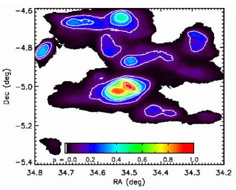
Figure 1: A probability map of clusters found by the Voronoi Tesselation method at redshift $z\sim 1.0$. Colours are normalised to the highest probability in the field.

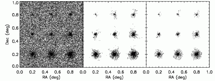
Figure 2: Example of simulated clusters superimposed on a galaxy background (left) as recovered by the Voronoi tessellation technique (middle) and the Friends-Of-Friends method (right). In this simulation the clusters are spherical with a total luminosity of 10,20,30,40,50,100,150,200,300 $L^{*}$ (top left to bottom right respectively) at $z=0.2$.

Friends-Of-Friends (FOF) algorithms are commonly used in spectroscopic galaxy surveys (e.g. Tucker et al., 2002; Ramella et al., 2002). A variant of this algorithm utilizing photometric redshifts was proposed by Botzler et al. (2004). They create redshift slices for their data cube and place the objects into the redshift slices according to their photometric redshift and error. The algorithm then links galaxy pairs within each slice that are closer to each other than some given linking distance, $D_{\rm Link}$, which is the projected separation of the galaxy pair. We use the empirically derived value of 0.175 Mpc for $D_{\rm Link}$ (proper coordinates) and consider a minimum of five galaxies in a group to be a cluster candidate.

An important difference between our algorithm and previous ones in the literature is the way we place the galaxies in the redshift slices. As we sample the full z-PDF to create MC-realisations of the three-dimensional galaxy distribution, we do not need to assign errors to individual galaxy redshifts. An object with a large redshift error will be distributed throughout many different slices in the 500 MC-realisations, and therefore not yield a significant contribution to the cluster candidates it is potentially found in. Thus there is no need to remove objects with large errors from the catalogue and no additional bias is introduced against faint objects with noisier photometry. A second modification to existing algorithms is the way we link up cluster candidates throughout the redshift slices. Instead of comparing individual galaxies in the clusters and linking up the clusters with corresponding members (see e.g. Botzler et al. 2004), we use probability maps of all redshift slices to locate likely cluster regions. This is discussed in the following section.

2.4 Probability maps and cross-correlation

Once the two cluster-detection methods have determined the cluster candidates in the redshift slices for all MC-realisations, we combine the MC-realisations to create a probability for both methods for each redshift slice. Figure  1 shows an example of a probability map: the VT cluster candidates in this slice at $z=1.0$ are contoured and coloured, with black through to red indicating low to high probability. This map is created by overplotting the extent of all cluster detections; the regions of the field that are found to be in a cluster in many MC-realisations are high-probability cluster locations. Since the error on the photometric redshifts of the galaxies is usually larger than the width of the redshift slices, each cluster candidate is typically found in several adjoining slices. We join the cluster candidates that occur in the same location in several slices by locating the peaks in the probability maps and inspecting the area within their contours in the adjoining redshift slices for cluster candidates. All the cluster candidates found in the same region in adjoining redshift slices are linked up into one final cluster; the final cluster redshift is determined by taking the mean of the redshift slices, weighted by the number of corresponding MC-realisations. We assign a reliability factor $F$ to each cluster by counting the total number of MC-realisations in which it occurs and dividing it by the total of 500 realisations. We then cross-correlate the cluster candidates output by the VT and FOF methods and take all cluster candidates that are detected in both with $F>0.2$. This is the final cluster sample.

3 Simulations

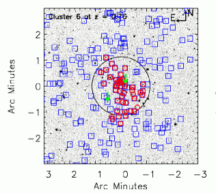
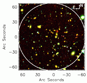
Figure 3: Cluster at $z=0.8$ detected with our cluster-finding algorithm from van Breukelen et al. (2006). Left: $K$-band image (UKIDSS-UDS); the large circle shows a 1 Mpc region around the cluster; the (blue) squares and (red) circles are cluster members as given by VT and FOF respectively. The (green) arrows point out galaxies with $z_{\rm spec}=0.87$. Middle: $Bz^{\prime}K$ image of the central 1 Mpc region. Right: colour-magnitude plot. The crosses are all galaxies within the central 1 Mpc region, otherwise the symbols are the same as in the left-hand panel. The grey band is the modelled red sequence.

To test the behaviour of the cluster-detection algorithm we run a set of simulations on mock-catalogues. These comprise ten random versions of clusters ranging in total luminosity from 10 $\rm L^{*}$ to 300 $\rm L^{*}$ and redshift $0.1<z<2.0$, superimposed on a galaxy distribution randomly placed in the field within the same redshift range. Realistic galaxy luminosities and number densities are determined by the $K$-band luminosity function of Cole et al. (2001) for the field-distribution and Lin et al. (2004) for the clusters, with the simplifying assumption of passive evolution with formation redshift $z_{form}=10$. A detection limit of $K_{lim,AB}=22.5$ is imposed to match the 5-$\sigma$ limit of the UDS EDR data (see section 4). The galaxies are spatially distributed within a cluster according to an NFW profile (Navarro, Frenk & White, 1997) with a cut-off radius of 1 Mpc. Figure 2 is an illustration of the detection of simulated clusters by the VT and FOF methods. It shows an example of a mock cluster catalogue with galaxy background (left) and the clusters as recovered by VT (middle) and FOF (right). The smallest cluster has a total luminosity of $L=10L^{*}$ and is detected by both methods.

When comparing the recovered cluster galaxies to the input mock cluster members, we see that VT tends to include all galaxies in a large area around the cluster core and the number of recovered cluster members, $N_{\rm gal,VT}$, is sensitive to the local field density. By contrast, the galaxy members recovered by FOF are more centrally concentrated and $N_{\rm gal,FOF}$ is consistent for mock clusters of the same total luminosity throughout the random realisations of the catalogues. Thus we can relate $N_{\rm gal,FOF}$ to the total luminosity of a detected cluster. We calculate $N_{\rm gal,FOF}$ by taking all galaxies that occur in the cluster in $>15\%$ of the MC-realisations in which the cluster itself is detected. The galaxies that appear in a smaller fraction of MC-realisations are very likely to be interlopers from different redshifts. Once we know $N_{\rm gal,FOF}$ for all simulated luminosities and redshifts, we derive functions of $N_{\rm gal}$ vs. $z$ for constant total cluster luminosity.

4 Application to UKIDSS-UDS data

To apply our cluster-detection algorithm to real observations, we used three sources of data in our published paper (van Breukelen et al. 2006): near-infrared $J$ and $K$ data from the UKIDSS Ultra Deep Survey Early Data Release (UDS EDR, Foucaud et al. 2006); 3.6$\mu$m and 4.5$\mu$m bands from the Spitzer Wide-area InfraRed Extragalactic survey (SWIRE, Lonsdale et al. 2005); and optical $BVRi^{\prime}z^{\prime}$ Subaru data over the Subaru XMM-Newton Deep Field (SXDF, Furusawa et al. in prep.). In this pilot study we restricted ourselves to a rectangular area of 0.5 square degrees, exhibiting a survey-depth of $K_{\rm AB,lim}=J_{\rm AB,lim}=22.5$ (UDS EDR 5$\sigma$ magnitude limits). We included objects with a detection in $i^{\prime}$, $J$ and $K$ in the galaxy catalogue and to exclude stars we impose a criterion of SExtractor stellarity index $<$ 0.8 in $i^{\prime}$ and $K$ (e.g. Bertin & Arnouts 1996). Subsequently we ran our photometric redshift code on this sample, resulting in a redshift catalogue of 19300 objects in the range $0.1\leq z\leq 2.0$.

4.1 Results: the UKIDSS-UDS cluster catalogue

Application of our cluster-detection algorithm to the redshift catalogue yielded 14 clusters at $0.61\leq z\leq 1.39$ (van Breukelen et al. 2006). Figure  3 shows one of the detected clusters: on the left a K-band image with the cluster members marked (FOF: circles, VT: squares); in the middle a $Bz^{\prime}K$ image of the central 1 Mpc region of the cluster; on the right a colour-magnitude diagram with the modelled red sequence overplotted.

To derive the clusters’ luminosity, we compared the results to the output of the simulations. We determined $N_{\rm gal,FOF}$ with $K<22.5$ (corresponding to the completeness limit) in the same way as for our simulated clusters; this allowed us to derive an approximate total luminosity to the cluster by interpolating between the lines of constant total luminosity in the $N_{\rm gal}-z$ plane found in our simulations. We found our clusters span the range of $10{\rm L^{*}}\mathrel{\hbox{\hbox to0.0pt{\hbox{\lower 2.0pt\hbox{$\sim$}}\hss}\raise 2.0pt\hbox{$<$}}}L_{\rm tot}\mathrel{\hbox{\hbox to0.0pt{\hbox{\lower 2.0pt\hbox{$\sim$}}\hss}\raise 2.0pt\hbox{$<$}}}50\rm L^{*}$; assuming $\frac{M/\rm M_{\odot}}{L/\rm L_{\odot}}=75h$ (Rines et al. 2001) this yields $0.5\times 10^{14}~{}{\rm M_{\odot}}\mathrel{\hbox{\hbox to0.0pt{\hbox{\lower 2.0pt\hbox{$\sim$}}\hss}\raise 2.0pt\hbox{$<$}}}M_{\rm cluster}\mathrel{\hbox{\hbox to0.0pt{\hbox{\lower 2.0pt\hbox{$\sim$}}\hss}\raise 2.0pt\hbox{$<$}}}3\times 10^{14}~{}\rm M_{\odot}$.

Clearly spectroscopic observations of these clusters are essential to confirm their reality, particularly for the high-redshift clusters which are cosmologically more valuable. In the near future highly multiplexed multi-object spectrometers on 8-metre class telescopes will provide the ideal opportunity for spectroscopical follow-up of high-redshift clusters. X-ray data and radio observations of the Sunyaev-Zel’dovich effect will also be able to convincingly confirm the reality of the clusters.

- [1] Bahcall, N. A. et al., 2003, ApJS, 148, 243
- [2] Bertin E., Arnouts S., 1996, A&AS, 117, 393
- [3] Bolzonella M., Miralles J.-M., Pell’o R., 2000, A&A, 363, 476
- [4] Botzler C. S. et al., 2004, MNRAS, 349, 425
- [5] Bruzual G., Charlot S., 2003, MNRAS, 344, 1000
- [6] Cole S. et al., 2001, MNRAS, 326, 255
- [7] Ebeling H., Wiedenmann G., 1993, PhRvE, 47, 704E
- [8] Eke V. R. et al., 1998, MNRAS, 298, 1145
- [9] Foucaud et al., 2006, preprint (astro-ph0606386)
- [10] Gal R. R., 2005, Guillermo Haro Summer School on Clusters, astro-ph/0601195
- [11] Goto et al., 2002, AJ, 123, 1807
- [12] Icke V., van de Weygaert R., 1987, A&A, 184, 16
- [13] Kim R. S. J. et al., 2002, AJ, 123, 20
- [14] Lawrence et al., 2006, preprint (astro-ph0604426)
- [15] Lin Y.-T., Mohr J. J., Stanford S. A., 2004, ApJ, 610, 745
- [16] Lonsdale C. J. et al., 2005, PASP, 115, 927
- [17] Lopes P. A. A. et al., 2004, AJ, 128, 1017
- [18] Navarro J., Frenk C., White S., 1997, ApJ, 490, 493
- [19] Ramella M. et al., 2001, A&A, 368, 776
- [20] Ramella M. et al., 2002, AJ, 123, 2976
- [21] Rines K. et al., 2001, ApJ, 561, L41
- [22] Silk J., Rees M. J., 1998, A&A, 331, 1
- [23] Stanford, S. A. et al., 2006, preprint (astro-ph0606075)
- [24] Tucker D. L. et al., 2000, ApJS, 130, 237
- [25] van Breukelen C. et al., 2006, preprint (astro-ph0608624)