Spectroscopic Binary Mass Determination using Relativity

Abstract

High-precision radial-velocity techniques, which enabled the detection of extrasolar planets are now sensitive to relativistic effects in the data of spectroscopic binary stars (SBs). We show how these effects can be used to derive the absolute masses of the components of eclipsing single-lined SBs and double-lined SBs from Doppler measurements alone. High-precision stellar spectroscopy can thus substantially increase the number of measured stellar masses, thereby improving the mass-radius and mass-luminosity calibrations.

1 Introduction

Precise radial-velocity (RV) measurements, with long-term precisions of a few meters per second, are now routinely obtained by several telescopes around the world. The most notable scientific achievement of precise RV measurements has been the detection of planets orbiting solar-type stars (Mayor & Queloz, 1995; Marcy & Butler, 1996). In this Letter we suggest another application of high-precision RVs, namely, the detection of relativistic effects in the Doppler shifts of close spectroscopic binary stars (SBs). Kopeikin & Ozernoy (1999) have already detailed the relativistic effects one expects to find in the Doppler measurements of binary stars. Here we focus on the effects that we expect to measure in SBs, and identify the additional information they provide.

The typical velocities of components of close binary stars can be as high as $150\,\mathrm{km\,s}^{-1}$, $\beta\equiv v/c\sim{\cal O}(10^{-4})$. The classical Doppler shift formula predicts a relative wavelength shift $\Delta\lambda/\lambda$ of order $\beta$. The next order corrections are of order $\beta^{2}\sim{\cal O}(10^{-8})$, which translate to ${\cal O}(1\,\mathrm{m\,s}^{-1})$. Terms of order $\beta^{3}$ are beyond foreseen technical capabilities. We thus limit our analysis to ${\cal O}(\beta^{2})$ effects — the transverse Doppler shift (time dilation) and the gravitational redshift. In principle, long term monitoring may reveal higher-order secular terms, such as the relativistic periastron shift or period decay through gravitational-wave radiation, but here we focus only on the periodic effects. These can be detected during relatively short observing runs, assuming the RV measurements are precise enough.

Recently, Zucker et al. (2006) have shown that the very same effects should be detectable in the stellar orbits around the black hole in the Galactic Center, after a decade of observations. The context we examine here is different, and the information that can be extracted may contribute to the statistics of close binary orbits.

2 Single-lined spectroscopic binary

The Keplerian RV curve of a single-lined spectroscopic binary (SB1) can be presented as:

$$V_{R1}=K_{1}\cos\omega\cos\nu-K_{1}\sin\omega\sin\nu+eK_{1}\cos\omega+V_{R0}\ ,$$ (1)

where $K_{1}$ is the primary star RV semi-amplitude, $\omega$ is the argument of periastron, $e$ is the eccentricity, $V_{R0}$ is the center-of-mass RV, and $\nu$ is the time-dependent true anomaly. The customary procedure to solve an SB1 is to fit this orbital model to the observed RV data. This fit is achieved through some optimization algorithm that scans the $(P,T,e)$ space (period, periastron time and eccentricity). For each trial set of values for these three parameters the algorithm produces the corresponding $\nu(t)$ and then solves analytically for $K_{C1}$($=K_{1}\cos\omega$), $K_{S1}$($=-K_{1}\sin\omega$), and $V_{R0}$, which appear linearly in the expression for $V_{R1}$.

In order to incorporate relativity into the observed RV curve of an SB1 we can use the models developed for analyzing binary pulsar timing data. Taylor & Weisberg (1989) present a detailed timing model of a relativistic binary pulsar, based on the relativistic celestial mechanics developed by Damour & Deruelle (1986). Besides the transverse Doppler shift and the gravitational redshift, relativity also introduces the Shapiro delay, periastron advance, and period decay through gravitational wave radiation. The formulae for the pulse delay in Taylor & Weisberg (1989) can be transformed to the RV domain by taking their time derivative. This calculation shows that the only terms of order $\beta^{2}$ are the gravitational redshift and the transverse Doppler shift, corresponding to the so-called ’Einstein delay’ in the pulsar timing model.

We now derive the two terms in a more didactic, albeit less rigorous fashion. In the center-of-mass frame, we can use energy conservation in the classic Keplerian solution to relate the transverse Doppler term to the radius vector of the observed component, $r_{1}$:

$$\frac{1}{2}\beta^{2}=\frac{1}{c^{2}}\frac{Gm_{2}^{3}}{\left(m_{1}+m_{2}\right)^{2}}\left(\frac{1}{r_{1}}-\frac{1}{2a_{1}}\right)$$ (2)

where $a_{1}$ is the orbital semi-major axis of the primary orbit, and $c$ is the speed of light. After some algebraic manipulation, we can estimate the corresponding modification to the measured RV from the transverse Doppler effect:

$$\Delta V_{\mathrm{TD}}=\frac{K_{1}^{2}}{c\sin^{2}i}\left(1+e\cos\nu-\frac{1-e^{2}}{2}\right)$$ (3)

where $i$ is the orbital inclination.

The gravitational redshift caused by the potential of the secondary component is inversely proportional to the separation of the two components:

$$\frac{\Delta\lambda}{\lambda}=\frac{Gm_{2}}{c^{2}\left(r_{1}+r_{2}\right)}$$ (4)

and the corresponding RV modification term from the gravitational redshift is:

$$\Delta V_{\mathrm{GR}}=\frac{K_{1}\left(K_{1}+K_{2}\right)}{c\sin^{2}i}\left(1+e\cos\nu\right)$$ (5)

After transformation to the observer frame, an additional term appears, related to the center-of-mass motion

$$\frac{V_{R0}}{c}K_{1}\left(\cos(\nu+\omega)+e\cos\omega\right)+\frac{V_{0}^{2}}{2c}\ ,$$ (6)

where $V_{0}$ is the magnitude of the full center-of-mass velocity vector.

In total, relativity adds the following ${\cal O}(\beta^{2})$ term to the measured $V_{R1}$:

$$\Delta V_{R1} = \frac{K_{1}}{c}\frac{1}{\sin^{2}i}\left[e(2K_{1}+K_{2})\cos\nu+(2K_{1}+K_{2})-\frac{1-e^{2}}{2}K_{1}\right]+$$

$$\frac{V_{R0}}{c}K_{1}\left(\cos\omega\cos\nu-\sin\omega\sin\nu+e\cos\omega\right)+\frac{V_{0}^{2}}{2c}$$

The resulting expression for the modified measured RV, $V_{R1}^{\prime}$, can now be easily simplified to:

$$V_{R1}^{\prime}=K_{C1}^{\prime}\cos\nu+K_{S1}^{\prime}\sin\nu+eK_{C1}^{\prime}+V_{R0}^{\prime}\ ,$$ (8)

by collecting together the constant terms, the terms proportional to $\cos\nu$, and those proportional to $\sin\nu$, and introducing the modified linear elements:

$$K_{S1}^{\prime} = -K_{1}\left(1+\frac{V_{R0}}{c}\right)\sin\omega$$ (9a)

$$K_{C1}^{\prime} = K_{1}\left[\left(1+\frac{V_{R0}}{c}\right)\cos\omega+\frac{e}{\sin^{2}i}\frac{2K_{1}+K_{2}}{c}\right]$$ (9b)

$$V_{R0}^{\prime} = V_{R0}+\frac{1-e^{2}}{\sin^{2}i}\frac{K_{1}}{c}\left(\frac{3}{2}K_{1}+K_{2}\right)+\frac{V_{0}^{2}}{2c}$$ (9c)

Equations 1 and 8 share exactly the same structure, and thus we can still apply the same fit procedure. However, the linear elements are more difficult to interpret now. The three quantities $K_{S1}^{\prime}$, $K_{C1}^{\prime}$, and $V_{R0}^{\prime}$ depend on the six elements $K_{1}$, $K_{2}$, $\omega$, $\sin i$, $V_{R0}$, and $V_{0}$. Thus, Equations 9 are under-determined and we cannot completely infer the six elements above, unless some additional independent information is available, or further assumptions are introduced.

Such independent information may be available through precise photometry of eccentric eclipsing binaries. There, the shapes and widths of the eclipses as well as the phase differences between primary and secondary eclipses can be used to estimate $\omega$ and $\sin i$. In this case, we may derive $K_{2}$ – the RV amplitude of the secondary:

$$K_{2}=\frac{2K_{S1}^{\prime}}{\sin\omega}-c\frac{\sin^{2}i}{e}\left(\cos\omega+\frac{K_{C1}^{\prime}}{K_{S1}^{\prime}}\sin\omega\right)\ .$$ (10)

In the above equation we neglected $V_{R0}$, as it contributes only higher order terms. By obtaining $K_{2}$ we effectively turn the binary into a double-lined spectroscopic binary (SB2), in which both $K_{1}$ and $K_{2}$ are measured. Together with the known inclination, we then obtain full knowledge of the component masses.

Curiously, another result of including the relativistic terms is that an eccentric binary should always display an apparent RV signature, even in the extreme case where the inclination is exactly zero and the orbit is observed face on. Since $K_{j}=2\pi a_{j}\sin i/(P\sqrt{1-e^{2}})$, $\sin i$ will cancel out in Equation 9b. Then $K_{C1}^{\prime}$ will be finite, while $K_{S1}^{\prime}=0$, and the apparent argument of periastron will be exactly $0\arcdeg$ or $180\arcdeg$. Thus, all the RV planet candidates whose arguments of periastra are close to these values, can in principle be binary stars observed exactly face on. Nevertheless, such small values of the inclination are extremely rare and this possibility is not realistic.

Equation 9c does not contribute any new useful information, since systematic effects in the measurement process such as spectral template mismatch are probably larger than the relativistic effects. In addition, the spectra are subject to gravitational redshift by the potential of the emitting star itself, and the typical uncertainties regarding its mass and radius are also larger than the effects we discuss here.

3 Double-lined spectroscopic binary

In the case of a Keplerian SB2, there are two sets of measured RVs. The two sets of RVs share the same fundamental orbital elements ($P$, $T$, $e$, $\omega$, and $V_{R0}$), and the only difference between them is their amplitudes $K_{1}$ and $-K_{2}$. The common procedure is to scan the space of the four parameters $(P,T,e,\omega)$ and then solve analytically for the three linear elements $K_{1}$, $K_{2}$, and $V_{R0}$. However, when we incorporate the relativistic corrections above, we see that we now have two RV curves with two different sets of derived amplitudes, arguments of periastra, and center-of-mass velocities. The two RV curves still share the same period, periastron time and eccentricity. We then have the following equations, corresponding to Equations 9a and 9b:

$$K_{S1}^{\prime} = -K_{1}\left(1+\frac{V_{R0}}{c}\right)\sin\omega$$ (11a)

$$K_{C1}^{\prime} = K_{1}\left[\left(1+\frac{V_{R0}}{c}\right)\cos\omega+\frac{e}{\sin^{2}i}\frac{2K_{1}+K_{2}}{c}\right]$$ (11b)

$$K_{S2}^{\prime} = -K_{2}\left(1+\frac{V_{R0}}{c}\right)\sin\omega$$ (11c)

$$K_{C2}^{\prime} = K_{2}\left[\left(1+\frac{V_{R0}}{c}\right)\cos\omega-\frac{e}{\sin^{2}i}\frac{K_{1}+2K_{2}}{c}\right]$$ (11d)

$V_{R0}$ appears in the four equations always divided by the speed of light. Thus we can safely use its approximate derived value, from either set of measured velocities , since the discrepancy will be only ${\cal O}(\beta^{3})$. We are left with four equations with four unknowns: $K_{1}$, $K_{2}$, $\omega$, and $\sin i$. Solution of this set of equations will yield a more accurate estimate of the first three unknowns, but more importantly, it will yield an estimate of $\sin i$. Retaining only leading order terms, we can arrive at the following solution:

$$\sin^{2}i=\frac{3e}{\omega_{2}^{\prime}-\omega_{1}^{\prime}}\frac{K_{S2}^{\prime}+K_{S1}^{\prime}}{c}\ ,$$ (12)

where

$$\omega_{j}^{\prime}=-\arctan\left(\frac{K_{S_{j}}^{\prime}}{K_{C_{j}}^{\prime}}\right)\ .$$ (13)

Thus, we see that relativity causes the apparent arguments of periastra to differ. Note that classically, there is no way to estimate $\sin i$ from pure RV data alone. The value of $\sin i$ is usually obtained only from the analysis of SBs that are eclipsing or astrometric binaries.

4 Discussion

We present here an approach to extract more information from RV data of a spectroscopic binary, based on the inclusion of relativistic effects. The practical potential lies in the time-dependent parts of the relativistic terms which are closely linked to the variation of the distance between the binary components. Thus, these terms are especially useful for orbits that are eccentric enough.

The approach is mainly useful in the case of SB2s, but precise photometry or astrometry may add the required information to utilize relativity in SB1s as well. Precise photometry space missions like MOST (Walker et al., 2003), CoRoT (Baglin, 2003), and Kepler (Basri, Borucki & Koch, 2005) may be able to provide precise enough measurements of $\omega$ and the inclination of eclipsing binaries from the analysis of their light curves.

In any case, it is essential that the data quality be high enough to be sensitive to variations of the required order, namely one meter per second or less. Currently, the best precision is obtained by the ESO HARPS fiber-fed echelle spectrograph, where the RV error can be as low as $1\,\mathrm{m\,s}^{-1}$ in certain cases and maybe even less (Lovis et al., 2005). In the future, much better precisions can be hoped for, on instruments designed for the “extremely large telescopes” (e.g., Pasquini et al., 2006).

To demonstrate the relevance of the suggested approach in real-life cases we chose to examine the SB2 12 Boo. Recently, Tomkin & Fekel (2006) published a precise solution of 12 Boo based on RVs obtained at the $2.1$-m telescope at the McDonald Observatory and at the Coudé feed telescope at Kitt Peak National Observatory, with RV precisions of $0.1$–$0.2$ km s^-1. The system has a period of $9.6$ days, eccentricity $0.2$, and both RV semi-amplitudes are close to $70$ km s^-1. These orbital parameters translate to an expected relativistic amplitude variation of about $10$ m s^-1 (Eq. 2). Furthermore, with a declination of $+25\arcdeg$, the star is observable by HARPS. Its brightness (5th magnitude) and spectral type (F9IV) make it fairly reasonable to expect a precision of $1$ m s^-1 with HARPS. We used the available $24$ RVs from Tomkin & Fekel (2006) and augmented them with only $3$ simulated HARPS measurements (assuming errors of $1$ m s^-1) , including the relativistic effects. For each assumed value of $\sin i$ we produced $1000$ sets of simulated measurements and solved for the orbital elements, using Equation 12 to estimate $\sin i$. Figure 1 shows the median of the derived values in solid line, and the $25\%$ and $75\%$ percentiles in dashed lines. The figure demonstrates that with reasonable efforts, $\sin i$ can be measured satisfactorily. In the worst case where $\sin i=1$, the standard deviation of the derived inclination is $0.14$ and a few more precise measurements can reduce this value significantly. An additional advantage of this test case is that the inclination of 12 Boo has already been measured by interferometry and is known to be $108\arcdeg$ (Boden et al., 2005). Thus if this test is performed, the derived $\sin i$ can be compared to the known value.

In real observations, more than three precise measurements may be needed in order to account for differences in zero points between instruments. Furthermore, The results depend crucially on the precision of $\omega_{1}^{\prime}$ and $\omega_{2}^{\prime}$, and a relative error of $\epsilon$ in $\omega_{2}^{\prime}-\omega_{1}^{\prime}$ will be translated to a relative error of $1.5\epsilon$ in the absolute masses. The few precise measurements can be scheduled to optimize the precision of those two elements (e.g. Ford, 2006).

Currently, precisions of a few meters per second are still difficult to obtain and besides using the best instruments available, there are also several limitations imposed by the star itself. Thus, early-type stars or rapid rotators, where the spectral lines are significantly broadened, do not lend themselves easily to high-precision RV measurements. Stellar oscillations and star spots are also a concern as they can cause apparent RV modulation. In addition, analyzing SB2s with the same level of precision as SB1s has not been easy until recently, when TODCOR (Zucker & Mazeh, 1994) was applied successfully to high-precision spectra by several teams (Zucker et al., 2004; Udry et al., 2004; Konacki, 2005).

The effects we have examined are most useful when the orbits are eccentric and the RV amplitudes are large enough. Large RV amplitudes are usually typical to close binaries, which are expected to have undergone orbital circularization and usually have vanishing eccentricities. However, eccentricity somewhat increases the RV amplitude, and even relatively wide binaries, with high enough eccentricities, can display quite large RV amplitudes.

Care must be taken to model correctly any other effects of order $\beta^{2}$ that might contaminate the data. One such effect is the light-travel-time effect. This effect can be easily approximated to the relevant order by adding the following term to $V_{R1}$ (and a corresponding one to $V_{R2}$):

$$\Delta V_{\mathrm{LT}}=\frac{K_{1}^{2}}{c}\sin^{2}\left(\nu+\omega\right)\left(1+e\cos\nu\right)$$ (14)

An effect which should be analyzed carefully is the tidal distortion of the stellar components, in particular close to periastron. This distortion may affect the spectral lines, introducing line asymmetry, which can bias the estimated Doppler shift. RV extrasolar planet surveys use the line-bisector analysis (e.g., Queloz et al., 2001) to quantify such time-dependent asymmetries. Further development of this technique may be the key to disentangle the tidal distortion and the relativistic effects.

One important application of the proposed method is to calibrate the low-mass end of the mass-luminosity relation, to better understand the stellar-substellar borderline. This mass regime is still poorly constrained, since low mass SB2s are quite rare due to the special photometric, spectroscopic and geometric requirements (Ribas, 2006). Large efforts are in progress to obtain accurate stellar masses in this regime, including adaptive optics, interferometry and in the future space interferometry (e.g., Henry et al., 2005). We propose a new, relatively accessible tool to accomplish this goal, where the only requirements are spectroscopic. Precise RVs for low-mass SB2s were already measured by Delfosse et al. (1999). Using the method presented here, their absolute masses may be derived with a relatively small observational effort. No other method exists yet to derive this information purely from RV measurements.

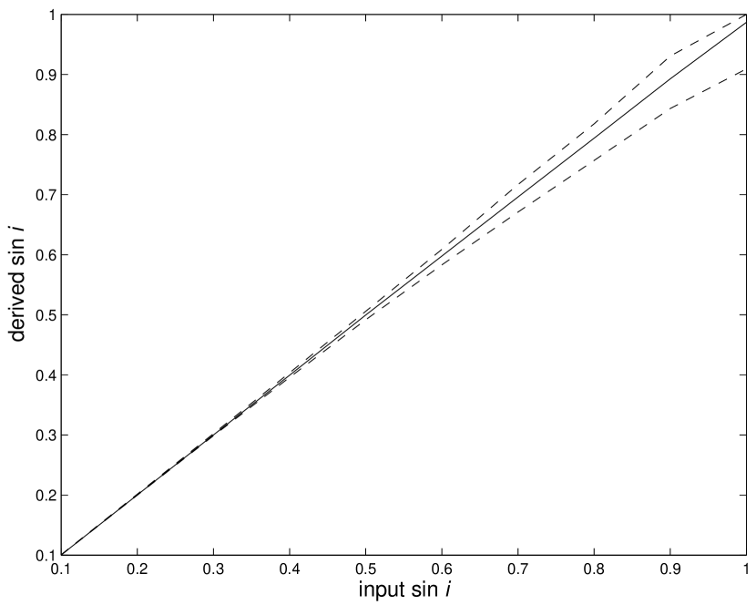
Figure 1: The results of simulations of 12 Boo including relativistic effects, assuming RV precision of $1$ m s^-1. The plot shows percentiles of the derived $\sin i$ against the input simulated value. The dashed lines represent the first and third quartile, and the solid line is the median.

References

- Baglin (2003) Baglin, A. 2003, Adv. Space Res., 31, 345
- Basri, Borucki & Koch (2005) Basri, G., Borucki, W. J., & Koch, D. 2005, New A Rev., 49, 478
- Boden et al. (2005) Boden, A. F., Torres, G., & Hummel, C. A. 2005, ApJ, 627, 464
- Damour & Deruelle (1986) Damour, T., & Deruelle, N. 1986, Ann. Inst. H. Poincaré (Physique Théorique), 44, 263
- Delfosse et al. (1999) Delfosse, X., Forveille, T., Beuzit, J.-L., Udry, S., Mayor, M., & Perrier, C. 1999, A&A, 344, 897
- Ford (2006) Ford, E. B. 2006, AJ, submitted (astro-ph/0412703)
- Henry et al. (2005) Henry, T. J., et al. 2005, BAAS, 37, 1356
- Konacki (2005) Konacki, M. 2005, ApJ, 626, 431
- Kopeikin & Ozernoy (1999) Kopeikin, S. M., & Ozernoy, L. M. 1999, ApJ, 523, 771
- Lovis et al. (2005) Lovis, C., et al. 2005, A&A, 437, 1121
- Marcy & Butler (1996) Marcy, G. W., & Butler, R. P. 1996, ApJ, 464, L147
- Mayor & Queloz (1995) Mayor, M., Queloz, D. 1995, Nature, 378, 355
- Pasquini et al. (2006) Pasquini, L., et al. 2006, in IAU Symp. 232, The Scientific Requirements for Extremely Large Telescopes, ed. P. Whitelock, B. Leibundgut, & M. Dennefeld (Cambridge: Cambridge Univ. Press), in press
- Queloz et al. (2001) Queloz, D., et al. 2001, A&A, 379, 279
- Ribas (2006) Ribas, I. 2006, Ap&SS, in press (astro-ph/0511431)
- Taylor & Weisberg (1989) Taylor, J. H., & Weisberg, J. M. 1989, ApJ, 345, 434
- Tomkin & Fekel (2006) Tomkin, J., & Fekel, F. C. 2006, AJ, 131, 2652
- Udry et al. (2004) Udry, S., Eggenberger, A., Mayor, M., Mazeh, T. & Zucker, S. 2004, Rev. Mexicana Astron. Astrofis., 21, 207
- Walker et al. (2003) Walker, G., et al. 2003, PASP, 115, 1023
- Zucker & Mazeh (1994) Zucker, S., & Mazeh, T. 1994, ApJ, 420, 806
- Zucker et al. (2006) Zucker, S., Alexander, T., Gillessen, S., Eisenhauer, F., & Genzel, R. 2006, ApJ, 639, L21
- Zucker et al. (2004) Zucker, S., Mazeh, T., Santos, N. C., Udry, S., & Mayor, M. 2004, A&A, 426, 695