The planet host star $\gamma$ Cephei: physical properties, the binary orbit, and the mass of the substellar companion

Abstract

The bright K1 III–IV star $\gamma$ Cep has been reported previously to have a companion in a $\sim$2.5-yr orbit that is possibly substellar, and also has a stellar companion at a larger separation that has never been seen. Here we determine for the first time the three-dimensional orbit of the stellar companion accounting also for the perturbation from the closer object. We combine new and existing radial velocity measurements (of both classical precision and high precision) with intermediate astrometric data from the Hipparcos mission (abscissa residuals) as well as ground-based positional observations going back more than a century. The orbit of the secondary star is eccentric ($e=0.4085\pm 0.0065$) and has a period $P=66.8\pm 1.4$ yr and a semimajor axis of $19.02\pm 0.64$ AU. We establish the primary star to be on the first ascent of the giant branch, and to have a mass of $1.18\pm 0.11$ M_☉, an effective temperature of $4800\pm 100$ K, and an age around 6.6 Gyr (for an assumed metallicity [Fe/H] = $+0.01\pm 0.05$). The unseen secondary star is found to be an M4 dwarf with a mass of $0.362\pm 0.022$ M_☉, and is expected to be $\sim$8.4 mag fainter than the primary in $V$ and $\sim$6.4 mag fainter in $K$. The minimum mass of the putative planetary companion is $M_{p}\sin i=1.43\pm 0.13$ M_Jup, the inclination angle of its orbit being unknown. Taking advantage again of the high-precision Hipparcos observations we are able to place a dynamical upper limit on this mass of 13.3 M_Jup at the 95% confidence level, and 16.9 M_Jup at the 99.73% (3$\sigma$) confidence level, thus confirming that it is indeed substellar in nature. The orbit of this object (semimajor axis $1.94\pm 0.06$ AU) is only 9.8 times smaller than the orbit of the secondary star (the smallest ratio among exoplanet host stars in multiple systems), but it is stable if coplanar with the binary.

1. Introduction

The bright evolved star $\gamma$ Cephei ($V=3.21$, SpT = K1 III–IV, $\alpha=23^{\rm h}39^{\rm m}21\fs 01$, $\delta=+77\arcdeg 37\arcmin 55\farcs 2$, J2000; also known as HD 222404, HR 8974, HIP 116727) is among the first objects to be subjected to high-precision radial-velocity measurements in an effort to discover substellar-mass companions around nearby stars (Campbell, Walker & Yang, 1988). This group of investigators (Campbell & Walker, 1979) pioneered the use of a hydrogen fluoride gas absorption cell on the Canada-France-Hawaii telescope (CFHT) and achieved internal errors around 13 m s^-1 for bright stars, inaugurating the era of Doppler searches that has been so successful in finding extrasolar planets in the last 10 years.

Small radial-velocity variations in $\gamma$ Cep were indeed seen by Campbell, Walker & Yang (1988) suggesting the presence of a Jupiter-mass object in a $\sim$2.5-yr orbit. Those variations with a semi-amplitude of only about 25 m s^-1 were superimposed on a much larger variation caused by a previously unnoticed stellar companion with a period of decades. However, the interpretation of the residual 2.5-yr variation as due to a planetary object was subsequently put in doubt by the same group (see Irwin et al., 1989; Walker et al., 1989, 1992). They argued that changes with a similar period were observed in a chromospheric activity indicator in $\gamma$ Cep (the Ca II $\lambda$8662 emission line index), and thus that the velocity variations were spurious and probably due only to changes in the spectral line profiles caused by surface inhomogeneities (spots) driven by stellar rotation. More recently the planetary interpretation was reinstated by Hatzes et al. (2003) on the basis of new high-precision velocity observations at the McDonald Observatory. They showed convincingly that the 2.5-yr variation is coherent in phase and amplitude throughout the entire 20-yr interval covered by the merged CFHT and McDonald data sets, as would be expected for Keplerian motion, and that no changes were observed in the spectral line bisectors. On the other hand, a careful re-analysis of the changes in the activity indicator reported by Walker et al. (1992) revealed that the periodicity of the Ca II $\lambda$8662 measurements (2.14 yr) is not only slightly different from that in the velocities, but it is transitory in nature, thus ruling out a connection.

$\gamma$ Cep also carries the distinction of being among the first planet host stars to be found in a binary system, which raises interesting issues related to the dynamical stability of such configurations. A recent study by Raghavan et al. (2006) points out that among the known planet host stars $\gamma$ Cep happens to be the system with the smallest ratio ($\sim$11) between the size of the binary orbit and the planetary orbit. However, the outer orbit is at present poorly known, and the secondary star is presumably very faint and has never been seen. Reported values for the binary period have ranged between 29.9 yr (Walker et al., 1992) and 66 yr (Griffin, Carquillat & Ginestet, 2002), and have been based on only part of the data available, in some cases spanning much less than a full cycle. A number of authors have carried out numerical investigations of the gravitational influence of the secondary star on the orbit of the planet (e.g., Dvorak et al., 2003; Thébault et al., 2004; Haghighipour, 2006), but have used rather different parameters for the binary or have pointed out the uncertainty in those elements as a limiting factor.

The motivation for this paper is thus threefold: $i$) To improve the determination of the orbit of the secondary star (including for the first time an estimate of the inclination angle, and of the mass of the secondary) in order to allow more definitive dynamical studies of the stability and evolution of the system. We do this by using all available radial velocity data for $\gamma$ Cep including new measurements reported here and other historical observations not previously used. We incorporate also astrometric measurements from the Hipparcos mission (“abscissa residuals”; ESA, 1997) as well as transit circle and other positional information spanning more than a century. $ii$) To carry out a critical review of previous studies of the physical properties of the primary star and use all available information to estimate its absolute mass, a key parameter influencing the mass of the substellar companion. $iii$) To place firm dynamical upper limits on the mass of this companion by taking advantage of the high-precision Hipparcos intermediate data and modeling the reflex motion of the primary star on the plane of the sky. We show that this modeling allows us to confirm the substellar nature of the companion, although it is not yet possible to rule out a mass in the brown dwarf regime.

2. Observational material

We describe here all spectroscopic and astrometric measurements of $\gamma$ Cep of which we are aware that have a bearing on the motion of the star, with the goal of combining them into a global orbital solution in §3.

2.1. Radial velocities

The high-precision Doppler measurements of $\gamma$ Cep have been described in detail by Hatzes et al. (2003). They consist of 4 separate data sets corresponding to different instrument configurations: three from the McDonald Observatory (referred to below as McDonald I, McDonald II, and McDonald III, following Hatzes et al., 2003), and one from the CFHT, which is the data set of Walker et al. (1992). The nominal precision of these measurements ranges from about 8 m s^-1 to $\sim$30 m s^-1, and they are all differential in nature as they rely on the use of telluric O₂ lines as the velocity metric, or on lines of hydrogen fluoride or iodine gas that play the same role. Taken together these velocities cover the interval 1981.4–2002.9, which includes periastron passage in the binary orbit. Hatzes et al. (2003) combined these data and solved simultaneously for the outer orbit and the orbit of the planet. The time span of the observations is less than half of their estimated binary period of 57 yr.

Beginning in the late 1970’s $\gamma$ Cep was monitored spectroscopically using more traditional means by Griffin, Carquillat & Ginestet (2002). To their own observations with several different instruments in Cambridge (England), Haute-Provence (France), and Victoria (Canada), they added a subset of the high-precision velocities mentioned above as well as other velocities collected from the literature in an effort to extend the time coverage and better constrain the outer orbit. These include measures published by Beavers & Eitter (1986) made in 1978–1980, and most importantly the velocities obtained at the Lick Observatory in 1896–1921 (Campbell & Moore, 1928). All these measurements were placed by Griffin, Carquillat & Ginestet (2002) on the same zero point (corresponding to their Cambridge instrument), and have formal uncertainties ranging from 0.2 km s^-1 to 0.9 km s^-1. We adopt these 77 measurements as published. These authors noted an unfortunate gap of some 50 years in the velocity coverage for $\gamma$ Cep that complicates the determination of the orbital period (see also §3.1). In order to distinguish between two possible periods (66 yr and 77 yr) allowed by the radial velocity data they used, they considered also other measurements from the literature in the interval 1902–1907 (Frost & Adams, 1903; Bélopolsky, 1904; Slipher, 1905; Küstner, 1908). They found that those velocities favored the 66-yr period, although they did not actually make use of them in their orbital solution because of their uncertain zero point.

Our own contribution to the observational material is twofold. On the one hand we have derived 3 new velocities for $\gamma$ Cep based on archival spectra collected at the Harvard-Smithsonian Center for Astrophysics (CfA) using an echelle spectrograph on the 1.5-m Tillinghast reflector at the F. L. Whipple Observatory. The nominal precision of these measurements is around 0.3 km s^-1 for a bright and sharp-lined star such as this. For details on the reduction procedures we refer the reader to the description by Torres, Neuhäuser & Guenther (2002). While this contribution is modest by comparison to the material described earlier, it does extend the time coverage to the end of 2004, and the velocities are on a well-defined system (see Stefanik, Latham & Torres, 1999; Latham et al., 2002).

Given the poor spectroscopic coverage prior to 1978, we carried out a careful search of the literature for additional measurements that might help constrain the outer orbit. Aside from the 1902–1907 sources mentioned above that were used only as supporting evidence by Griffin, Carquillat & Ginestet (2002), a number of other velocity sources were found but their zero points are generally unknown, so the measurements cannot be combined at face value. Thus as a second contribution we relied on the extensive CfA database of $\sim$$250,\!000$ spectra to place all of those scattered measurements of $\gamma$ Cep onto a uniform frame of reference. This was accomplished by using measurements for other stars also reported in each of these sources, and comparing them with newly derived velocities for those same “standards” from CfA spectra obtained at one time or another over the past 25 years. Details of this procedure are provided in the Appendix. Of particular relevance are the $\gamma$ Cep measurements by Kjærgaard et al. (1981) made in 1977, Snowden & Young (2005) in 1972–1974, Boulon (1957) in 1955, and Harper (1934) in 1921. The precision of those velocities ranges from 0.5 km s^-1 to about 1.9 km s^-1. We list them in Table 1 along with our own measurements, all on the CfA system.

Despite our attempts to establish their zero points, two of the sources of historical velocities showed large discrepancies when compared with other data taken at similar times, or presented other problems. The series of measurements by Bélopolsky (1904) contains only 5 other stars usable as standards, and the offset required to place those velocities on the CfA system has the largest uncertainty ($\sim$1 km s^-1). The corrected $\gamma$ Cep velocities from 1903 are some 3 km s^-1 too high. Three velocities measured at Mt. Wilson Observatory in 1915–1917 (Abt, 1973) show the largest spread of any data set (4 km s^-1). The zero point of those measurements is very difficult to establish because of the variety of instruments and telescopes used, which are not always indicated in the original publication. The average of the corrected velocities for $\gamma$ Cep shows a discrepancy of 5 km s^-1 relative to others made within a few years. We have therefore not made use of either of these two data sets in our orbital solution described in §3. Several high-dispersion plates of $\gamma$ Cep were obtained by Koelbloed & van Paradijs (1975) in 1963–1964, a critical time in the observational history of this object, but unfortunately the authors appear not to have measured radial velocities. Finally, Ruciński & Staniucha (1981) published a velocity measurement for $\gamma$ Cep made in 1979, but all of the other stars reported in their paper happen to be variable, and so cannot be used as standards.

2.2. Astrometry

$\gamma$ Cep was observed by the Hipparcos satellite between 1989 and 1993 (ESA, 1997). These accurate one-dimensional astrometric measurements were used by the Science Team to derive the position, proper motion, and trigonometric parallax of the object ($\pi_{\rm HIP}=72.50\pm 0.52$ mas) as reported in the main catalog. The astrometric solution revealed a measurable acceleration on the plane of the sky (proper motion derivatives) in the amount of $d\mu_{\alpha}/dt=+1.51\pm 1.12$ mas yr^-2 in Right Ascension and a more significant $d\mu_{\delta}/dt=+6.10\pm 1.11$ mas yr^-2 in Declination. This acceleration is of course due to the binary nature of the object, and was accounted for in deriving the parallax.

As we demonstrate below, the binary motion at the epoch of the Hipparcos observations is such that we expect some curvature on the plane of the sky that should be detectable in the measurements. We have therefore made use of these observations (available in the form of “abscissa residuals”) in our orbital solution described below, since they are complementary to the spectroscopic observations and provide new information. A total of 76 such measurements were obtained by the two independent data reduction consortia (ESA, 1997), and the median error for a single measurement is 1.9 mas.

Because of the relatively short time span of these observations compared to the binary orbital period, it is almost certain that part of the orbital motion has been absorbed into the proper motion components reported by Hipparcos. This is in fact a way in which many long-period binaries have been discovered in the past, on the basis of the apparent variability of their proper motions when computed at different epochs (see, e.g., Wielen et al., 1999; Gontcharov, Andronova & Titov, 2000; Makarov & Kaplan, 2005). Precisely this effect was pointed out for $\gamma$ Cep by Heintz (1990), who noticed a significant change mostly in $\mu_{\delta}$ over several decades. Therefore, to make proper use of the Hipparcos intermediate data to extract information on the binary orbit it is necessary to constrain the proper motion by other means in order to model the orbital motion without risking systematic errors.

Initially we considered using the proper motion for $\gamma$ Cep reported in the Tycho-2 catalog (Høg et al., 2000a), which relies on ground-based positional measurements made over many decades and is constrained at the recent epoch by the Tycho-2 position. This long baseline presumably averages out any perturbations due to orbital motion if the period is significantly shorter than this. The Tycho-2 proper motion is in fact quite different from the Hipparcos determination, which is effectively “instantaneous” at the mean epoch $\sim$1991.25. In the case of $\gamma$ Cep, however, the orbital period is not negligible compared to the time span, and we were concerned that $\mu_{\alpha}$ and $\mu_{\delta}$ might be biased. Evidence that the orbital motion is detectable in the individual positional measurements from transit circle observations was indeed presented by Gontcharov, Andronova & Titov (2000), who inferred from them a period of about 45 yr for the binary. We therefore chose to make use of the individual positions from ground-based catalogs going back to 1898, kindly provided by S. Urban of the U.S. Naval Observatory (USNO). Additional measurements from the Carlsberg Meridian Catalogs (CMC; see, e.g., Carlsberg Meridian Catalogue, 1989) were provided by G. Gontcharov (Pulkovo Observatory) or obtained from the literature. All of these measurements have been reduced to the International Celestial Reference Frame (ICRF), effectively represented in the optical by the Hipparcos catalog, and their nominal precision varies between about 50 and 500 mas (see Høg et al., 2000b). We list them in Table 2.

3. Orbital solution

The combination of the radial velocity mesurements and the astrometry makes it possible to derive the complete set of elements describing the binary orbit in $\gamma$ Cep. The inclination angle is of particular interest because when combined with the spectroscopic mass function it provides the information needed to compute the mass of the secondary star, given an estimate of the primary mass. The substellar companion to the primary introduces additional components of motion that we model simultaneously. Given that the outer orbit is an order of magnitude larger than the inner orbit (see §1), to first order we assume here that they are decoupled, i.e., that the outer one may be treated as corresponding to a “binary” composed of the secondary star (B) and the center of mass of the inner pair (A). Orbital elements that refer to the outer orbit are indicated below with the subindex “AB”, and those pertaining to the inner orbit are distinguished with a subindex “A”. The primary star itself is referred to as “Aa” following the traditional spectroscopic notation, and the planet (indistinctly called also ‘substellar companion’) as “$p$”, for simplicity.

The radial velocities allow us to solve for the period, center-of-mass velocity of the (triple) system, eccentricity, velocity semi-amplitude, longitude of periastron, and time of periastron passage in the outer orbit: {$P_{\rm AB}$, $\gamma$, $e_{\rm AB}$, $K_{\rm A}$, $\omega_{\rm A}$, $T_{\rm AB}$}. The high-precision velocities constrain the spectroscopic elements of the inner (planetary) orbit: {$P_{\rm A}$, $e_{\rm A}$, $K_{\rm Aa}$, $\omega_{\rm Aa}$, $T_{\rm A}$}. Because the high-precision velocities are differential, an offset must be determined to place them on the frame of the absolute velocities, for which we have chosen the Griffin data set as the reference. We therefore solved for 4 additional parameters representing these offsets, one for each data set: $\Delta RV_{1}$, $\Delta RV_{2}$, and $\Delta RV_{3}$ for the groups referred to as McDonald I, McDonald II, and McDonald III (see §2.1), and $\Delta RV_{4}$ for the CFHT data set. The CfA velocities and other historical data sets placed on the CfA system were considered as a single group, and one additional parameter $\Delta RV_{5}$ was included to represent the shift relative to Griffin.

Preliminary estimates suggested the secondary star is very small compared to the primary, and we may assume here that it contributes no light. The Hipparcos observations therefore refer strictly to the primary as opposed to the center of light, and provide a constraint on the orientation of the outer orbit (inclination angle $i_{\rm AB}$ and position angle of the ascending node $\Omega_{\rm AB}$, referred to the equinox of J2000) as well as on the angular scale of the orbit of the inner binary relative to the barycenter ($a^{\prime\prime}_{\rm A}$). We show below that the astrometric measurements do not, however, resolve the wobble of the primary star caused by the planet. We point out also that there are no available measurements of the relative position between the two stars, since the secondary has never been resolved. The use of the Hipparcos measurements in the global solution introduces several other parameters that must be solved for, including corrections to the catalog values of the position of the barycenter ($\Delta\alpha^{*}$, $\Delta\delta$) at the mean reference epoch of 1991.25, and corrections to the proper motion components ($\Delta\mu_{\alpha}^{*}$, $\Delta\mu_{\delta}$). In principle we also need to solve for a correction to the Hipparcos parallax. However, the fact that the spectroscopic elements of the outer orbit are solved for at the same time introduces a redundancy, and the parallax (which in this case would be termed an “orbital” parallax) can be expressed in terms of other elements as

$$\pi=1.0879\times 10^{4}{a^{\prime\prime}_{\rm A}\sin i_{\rm AB}\over P_{\rm AB}~{}K_{\rm A}\sqrt{1-e_{\rm AB}^{2}}}~{},$$ (1)

where the period is given in days and $K_{\rm A}$ in km s^-1. We have therefore chosen to eliminate the parallax correction as an adjustable parameter.

By combining complementary observations of different kinds the global solution is strengthened. The ground-based positional measurements provide the tightest constraint on the proper motion and position of the barycenter. This breaks the strong correlation between proper motion and orbital motion in the Hipparcos observations, and enables those measurements to provide a constraint on the angular scale and orientation of the outer orbit, even though their coverage is only a small fraction of the orbital period. Some information on the scale and orientation, as well as on the outer period, is provided also by the positional measurements, while the velocities contribute most of the weight to the period, shape, and linear scale of the binary orbit. The elements of the inner orbit are constrained only by the high-precision velocity measurements, and are only weakly dependent on the outer orbit. Light-travel effects in the inner orbit are negligibly small. The formalism for incorporating the abscissa residuals from Hipparcos into the fit follows closely that described by van Leeuwen & Evans (1998) and Pourbaix & Jorissen (2000), including the correlations between measurements from the two independent data reduction consortia (ESA, 1997). In using the ground-based catalog positions the parallactic motion was accounted for in our model, given that the precision of some of the more recent measurements is comparable to the parallax.

Altogether there are 23 unknowns that we solved for simultaneously, using standard non-linear least-squares techniques (Press et al., 1992, p. 650). The solution converged quickly from initial values of the elements chosen from preliminary fits or by an extensive grid search, and experiments in which we varied the initial values within reason yielded the same results. A total of 446 individual observations were used from 10 different data sets, as follows: 107 classical radial velocities (77 from Griffin, 30 from CfA and other literature sources), 199 high-precision velocities (68 from CFHT, 43 from McDonald I, 49 from McDonald II, and 39 from McDonald III), 76 one-dimensional Hipparcos measurements, and 64 ground-based catalog coordinates (split into two data sets of 15 and 17 pairs of Right Ascension and Declination measurements). Weights were assigned to the measurements according to their individual errors. Since internal errors are not always realistic, we adjusted them by applying a scale factor in such a way as to achieve a reduced $\chi^{2}$ value near unity separately for each data set. This was done by iterations. These scale factors were all close to unity for most of the velocity sets, and somewhat larger for some of the ground-based catalog positions.

The results are given in Table 3, along with derived quantities such as the position of the barycenter at the mean epoch of the Hipparcos catalog (1991.25), the parallax and proper motion components, and the mass function of the stellar binary. Other derived quantities are described below. The elements of the planetary orbit are not significantly different from those reported by Hatzes et al. (2003) since that orbit depends essentially only on the high-precision velocities, for which we used the same data they used. The parallax is also not appreciably different from the Hipparcos value, although our uncertainty is somewhat smaller. The proper motion components, on the other hand, are considerably different from their catalog values, as anticipated above.

The radial velocity measurements are represented graphically in Figure 1. The top panel shows only the classical measurements. The small undulations in the computed curve are produced by the wobble of the primary star with the 2.47-yr period of the substellar companion. Although the phase coverage in the outer orbit is incomplete, the period of the binary is fairly well established thanks in part to the very high precision of the McDonald and CFHT data (see also §3.1). These are shown separately in the lower panel, where the error bars are smaller than the size of the points. The reflex motion of the primary due to the substellar companion is shown as a function of orbital phase in Figure 2, where the motion in the outer orbit has been subtracted from the individual data sets. The residuals from the new CfA velocities and from other values from the literature sources placed on the same system are given in Table 1.

The path of $\gamma$ Cep on the plane of the sky is represented in Figure 3, where the axes are parallel to the Right Ascension and Declination directions. The solid curve is the result of the contributions from the annual proper motion (arrow), the parallactic motion, and the motion in the binary. The wobble due to the substellar companion is negligible on the scale of this figure (see also §5). The predicted location of the one-dimensional Hipparcos observations is indicated by the dots on the curve. As stated earlier, their typical uncertainty is 1.9 mas. For illustration purposes, the dotted line in the figure starting at the location of the first Hipparcos observation shows the path the star would follow without the perturbation from the orbital motion in the binary.

The orbit of the primary star in $\gamma$ Cep around the center of mass of the binary is shown in Figure 4, with a semimajor axis of about 325 mas. The direction of motion is retrograde (arrow). The intersection between the orbital plane and the plane of the sky (line of nodes) is represented by the dotted line. The section of the orbit covered by the Hipparcos mission is indicated with filled circles, and the open circle labeled “P” represents periastron. A close-up of the area around the Hipparcos observations is shown in Figure 5. Because these measurements are one-dimensional in nature, their exact location on the plane of the sky cannot be shown graphically. The filled circles represent the predicted location on the computed orbit. The dotted lines connecting to each filled circle indicate the scanning direction of the Hipparcos satellite for each measurement, and show which side of the orbit the residual is on. The short line segments at the end of and perpendicular to the dotted lines indicate the direction along which the actual observation lies, although the precise location is undetermined. Occasionally more than one measurement was taken along the same scanning direction, in which case two or more short line segments appear on the same dotted lines.

The motion of $\gamma$ Cep A in the binary orbit is discernible in the ground-based catalog measurements taken over the last century, although only in the Declination direction. This is illustrated in Figure 6. The amplitude of motion in the R.A. direction is much smaller because of the orientation of the orbit, which is mostly North-South. The more recent measurements since 1980 are much more precise. That section of the orbit is shown on a larger scale in Figure 7. The residuals of all ground-based measurements from our orbital solution are given in Table 2.

3.1. The constraint on the binary period

The poor observational coverage of $\gamma$ Cep prior to 1980 has made it difficult to establish the period of the outer orbit in previous studies, particularly since the secondary star has never been resolved. Walker et al. (1992) gave a rough estimate of 29.9 yr based on only 10 yr of high-precision velocity coverage. Gontcharov, Andronova & Titov (2000) used the ground-based catalog positions spanning a little less than six decades and inferred a period of 45 yr. A re-reduction of those same data (G. Gontcharov 2006, private communication) does not show that periodicity as clearly, however. The radial-velocity study by Griffin, Carquillat & Ginestet (2002) took advantage of some of the historical measurements going back more than 100 yr, and found that a 50-yr gap in the data near the middle of the last century allowed two possible periods giving fits of similar quality: $\sim$66 yr and $\sim$77 yr. On the basis of other observational evidence they chose the short orbital period. Hatzes et al. (2003) used 20 yr worth of high-precision velocity measurements and derived a period of 57 yr.

The simultaneous use of all of the above measurements, and the addition of other observations (including more recent velocities as well as historical velocities, and the Hipparcos measurements), have allowed us to finally constrain the binary period without ambiguity to a value of 66.8 yr, thus proving Griffin, Carquillat & Ginestet (2002) essentially correct. To illustrate the improvement brought about by the added observations, we have recreated the fit by Griffin, Carquillat & Ginestet (2002) by using the same set of observations they used, ignoring the velocity perturbation from the substellar companion, as they did. In Figure 8 we show the reduced $\chi^{2}$ of the fit for a range of fixed orbital periods, with the remaining orbital elements adjusted as usual to minimize $\chi^{2}$. We then repeated this exercise using the data that went into our own solution, this time accounting properly for the planetary companion. The dashed curve corresponding to the solution by Griffin, Carquillat & Ginestet (2002) shows two local minima at $\sim$66 yr and $\sim$77 yr, as found by those authors. The solid curve corresponding to the solution in this paper that includes all available observations has a single minimum at 66.8 yr. The formal uncertainty in this value is 1.4 yr, or 2%.

4. Physical properties of the primary and secondary stars

In order to take full advantage of the orbital solution presented above and estimate the mass of the unseen secondary star, as well as to place limits on the mass of the substellar companion, we require an estimate of the mass of the primary star itself ($M_{\rm Aa}$). Mass estimates in the literature for $\gamma$ Cep have varied by more than a factor of two (between $\sim$0.8 M_☉ and $\sim$1.7 M_☉), which is somewhat surprising for such a bright and well-studied star but may perhaps be explained by its present evolutionary state and other uncertainties (see below). We wish to constrain it to much better than this to avoid propagating the uncertainty to other quantities that depend on the mass. In this section we therefore examine the available observational material carefully and critically, making use of current stellar evolution models to arrive at the best possible estimate for $M_{\rm Aa}$. We discuss some of the other estimates as well in an attempt to understand the differences.

The brightness of $\gamma$ Cep has made it an easy target for spectroscopic studies to determine both the effective temperature and chemical composition of the star. These, along with other properties, are essential in order to estimate its absolute mass. In Table 4 we have collected the results of nearly two dozen separate investigations carried out over the past 40 years. We consider here only determinations of $T_{\rm eff}$ and [Fe/H] that are purely spectroscopic. Our own temperature estimate from the spectra described in §2.1 is listed as well (see §A for the details of our procedures). For the most part the 22 independent metallicity determinations show reasonable agreement within the errors, and yield a weighted average of [Fe/H] = $+0.01\pm 0.02$, or very nearly solar. Further comments on this value are given below. The weighted average effective temperature is $T_{\rm eff}=4852\pm 26$ K from 9 spectroscopic measurements including our own. The uncertainties given here are statistical errors that account for the different weights as well as the scatter of the individual [Fe/H] and $T_{\rm eff}$ measurements, but not for possible systematics. In the following we adopt for these averages more conservative errors of 0.05 dex and 100 K, respectively.

Temperature estimates for the star have been derived on numerous occasions also from color indices in a variety of photometric systems. In order to bring homogeneity to this information we have compiled the available photometry for $\gamma$ Cep in eight different systems (Johnson, Strömgren, Vilnius, Geneva, Cousins, DDO, 2MASS, and Tycho) mostly from the photometric database maintained by Mermilliod, Mermilliod & Hauck (1997), and we have used the color/temperature calibrations for giant stars from Ramírez & Meléndez (2005) for 13 different photometric indices. Interstellar reddening has been ignored here in view of the close distance to the star (13.8 pc), but we have accounted for the very small metallicity correction in each calibration based on the discussion above. The results are collected in Table 5, where the uncertainty of each temperature estimate includes the contribution from photometric errors as well as the statistical uncertainty of the calibration, added in quadrature. The weighted average of these determinations is $T_{\rm eff}=4754\pm 17$ K, although we prefer 100 K as a more realistic error to account for unquantified systematics. The spectroscopic and photometric temperature estimates thus differ by only 100 K, and we adopt here the compromise value of $T_{\rm eff}=4800\pm 100$ K.

Two additional properties of the star that can be determined very accurately are the absolute visual magnitude and the linear radius. The absolute magnitude follows from $V=3.213\pm 0.007$ (Mermilliod, Mermilliod & Hauck, 1997) and our parallax for the system (Table 3), and is $M_{V}=2.521\pm 0.014$. The angular diameter of $\gamma$ Cep has been measured directly with high precision by Nordgren et al. (1999) using the Navy Prototype Optical Interferometer, and is $\phi=3.24\pm 0.03$ mas (limb-darkened value). Combined once again with our parallax, this measurement yields the linear radius as $R=4.790\pm 0.052$ R_☉, which has a formal precision just over 1%.

In Figure 9 we compare the measured temperature and absolute visual magnitude of the star with evolutionary tracks from the series by Yi et al. (2001) and Demarque et al. (2004) for the composition established above. Tracks are labeled with the mass in solar units. The star is seen to be in the first ascent of the giant branch. The shaded error box is shown more clearly in the inset, which suggests a mass for $\gamma$ Cep slightly over 1.2 M_☉ and an uncertainty in that value determined almost entirely by the temperature error at this fixed metallicity. If the radius is used instead of the temperature, the constraint on the mass is considerably improved because of the smaller relative error of $R$. This is shown in Figure 10, which indicates a mass also close to 1.2 M_☉, consistent with the previous figure. In both cases the uncertainty in the metallicity is also important, as a change in [Fe/H] shifts the tracks essentially horizontally.

The optimal value of the mass is one that yields the best simultaneous match to the four measured quantities ($T_{\rm eff}$, [Fe/H], $M_{V}$, and $R$) within their stated errors. To determine this value, as well as its uncertainty, we computed by interpolation evolutionary tracks in a fine grid for a range of masses and also a range of metallicities within the observational uncertainty of [Fe/H]. At each point along the tracks we compared the predicted stellar properties with the measurements, and recorded all models that agree with the observations within their errors. All such models are displayed in Figure 11 in a mass/age diagram. It is seen that at each mass the range of allowed ages is very narrow. The best match is for a mass of $M_{\rm Aa}=1.18_{-0.11}^{+0.04}$ M_☉, and the corresponding evolutionary age is $6.6_{-0.7}^{+2.6}$ Gyr. All four measured quantities are reproduced to well within their errors (better than 0.3$\sigma$), an indication that they are mutually consistent. The surface gravity predicted by the best model is $\log g=3.15$. An independent age estimate was obtained by Saffe, Gómez & Chavero (2005) based on the chromospheric activity indicator $\log R_{\rm HK}^{\prime}=-5.32$. Their result (6.39 Gyr) using the calibration by Rocha-Pinto & Maciel (1998) agrees very well with ours formally, although chromospheric ages for older objects tend to be rather uncertain.

There are significant differences between our mass and other recent estimates. Almost all of them rely on evolutionary models and use different combinations of observational constraints. For example, Fuhrmann (2004) derived a value of 1.59 M_☉ with a formal error less than 10%, from a fit to the effective temperature and bolometric magnitude (derived using the Hipparcos parallax) for a fixed metallicity that is higher than ours (see Table 4). This mass estimate was adopted by Hatzes et al. (2003) to infer the minimum mass of the substellar companion to $\gamma$ Cep. Affer et al. (2005) obtained an even larger primary mass of 1.7 M_☉ (no uncertainty given) from a fit to their own $T_{\rm eff}$ and $M_{V}$ (also based on the Hipparcos parallax), using their [Fe/H] determination that is again higher than ours. Allende Prieto & Lambert (1999) used $M_{V}$ and $B-V$ directly and inferred $M_{\rm Aa}=1.33$ M_☉, but apparently made no use of any measured metallicity. A lower mass than ours ($M_{\rm Aa}=1.0\pm 0.2$ M_☉) was derived by Luck & Challener (1995) from the luminosity and temperature they determined for $\gamma$ Cep, along with their [Fe/H] value, which is close to solar. Głȩbocki (1972) obtained 1.5 M_☉ employing a similar method, but adopted a metallicity much lower than ours. Except for the latter study, the evolutionary models used by most of these authors are similar enough that the differences in mass must be due in large part to the observational constraints, particularly the temperature and metallicity. We note also that none of these studies have made use of the measured angular diameter of the star, which appears to be very accurate. An entirely different approach was followed by Gratton et al. (1982), who inferred a mass from their spectroscopic $\log g$ determination along with a linear radius derived from surface brightness relations ($R=6.5$ R_☉). Their value is $M_{\rm Aa}=0.89\pm 0.19$ M_☉.

The larger estimates of $M_{\rm Aa}$ tend to be those based on hotter temperatures and also higher metallicities. Furthermore, a look at Table 4 shows that while most of the metallicity determinations for $\gamma$ Cep are close to solar, all the higher values have been reported only in the last few years, and they tend to go together with hotter temperatures (see Figure 12). We note in this connection that $\gamma$ Cep has been considered a member of a group of evolved stars displaying CN bands that are stronger than usual (‘strong-CN stars’, or ‘very-strong-lined stars’; see, e.g., Spinrad & Taylor, 1969; Keenan, Yorka & Wilson, 1987). It was classified by the latter authors as K1 III-IV CN 1, which corresponds only to a marginal strong-CN star. These objects have had a controversial history, occasionally having been considered to be super-metal-rich. Other studies have disputed this, however. For example, some of the giants in the open cluster M67 have been found to have strong CN features even though the chemical composition of this cluster is believed to be essentially solar (see, e.g., Luck & Challener, 1995). We refer the reader to the latter work (and references therein) for an excellent summary of the subject and a list of possible explanations for the CN phenomenon.

As tempting as it may be to place higher confidence in some of the more recent [Fe/H] studies that have found a metal-rich composition for $\gamma$ Cep, it is difficult to ignore the large body of equally careful determinations yielding a composition closer to solar. This includes the recent work of Franchini et al. (2004), which not only gives a slightly subsolar metallicity but also happens to have the smallest formal uncertainty; their result is [Fe/H] = $-0.066\pm 0.034$. As a test we repeated the comparison with stellar evolution models described earlier, but adopting the spectroscopic temperature and metallicity determinations of each of the recent studies that give super-solar abundances. In no case did we find a model that is simultaneously consistent with all four of the quantities $T_{\rm eff}$, [Fe/H], $M_{V}$ and $R$, within their uncertainties. We are led to conclude, therefore, that the chemical composition of $\gamma$ Cep is not significantly higher than solar, and we adopt in the following the mass we determined above with the most conservative of the asymmetric error bars: $M_{\rm Aa}=1.18\pm 0.11$ M_☉.

With this value and the mass function from our orbital solution the mass of the unseen stellar companion is $M_{\rm B}=0.362\pm 0.022$ M_☉, where the error is computed from the full covariance matrix resulting from our fit (including cross-terms) and accounts also for the primary mass uncertainty, which represents the dominant contribution. Thus the secondary is most likely a late-type star of spectral type approximately M4. The angular semimajor axis of the relative orbit between the primary and secondary becomes $a^{\prime\prime}_{\rm AB}=1.382\pm 0.047$ arcsec, which corresponds to $19.02\pm 0.64$ AU.

With the secondary mass known, it is of interest to compute its brightness relative to the primary in order to assess the chance of detecting it directly, most likely in the infrared. The brightness measurements of the primary itself in the near infrared are rather uncertain because the star saturated the 2MASS detectors (see Table 5). From our best model fits we derive absolute magnitudes of $M_{H}\simeq 0.28$ and $M_{K}\simeq 0.19$ in the Johnson system, which are actually consistent with the values inferred from the 2MASS photometry within their large errors. The brightness of the secondary star may be estimated also from stellar evolution models. For this we have used the calculations by Baraffe et al. (1998), since those of Yi et al. (2001) are not intended for low-mass stars. For the age we established above we obtain $M_{V}\simeq 10.92$, $M_{H}\simeq 6.83$, and $M_{K}\simeq 6.56$, which we have placed on the same photometric system as Yi et al. (2001) following the prescription by Bessell & Brett (1988). Thus, the secondary is expected to be $\sim$8.4 mag fainter than $\gamma$ Cep A in $V$, $\sim$6.6 mag fainter in $H$, and $\sim$6.4 mag fainter in $K$.

The orbital elements in Table 3 allow the relative position of the unseen secondary to be predicted. We note, however, that the scale of the relative orbit still depends critically on the assumed primary mass as $(M_{\rm Aa}+M_{\rm B})^{1/3}$, in which the secondary mass itself scales as $(M_{\rm Aa}+M_{\rm B})^{2/3}$. As seen earlier $M_{\rm Aa}$ is quite sensitive to the adopted temperature and metallicity. A dynamical (hypothesis-free) estimate of the masses of both stars and a direct measure of the semimajor axis $a^{\prime\prime}_{\rm AB}$ will be possible once $\gamma$ Cep B is detected and its path around the primary measured over at least a portion of the orbital cycle.

5. The mass of the planetary companion

The reflex motion of the primary star along the line of sight in response to the putative substellar companion leads to a mass function of $f(M_{p})=(1.83\pm 0.32)\times 10^{-9}$ M_☉ from our orbital fit. With the adopted value of $M_{\rm Aa}$ this corresponds to $M_{p}\sin i_{\rm A}=1.43\pm 0.13$ M_Jup, which is only slightly smaller than the value $M_{p}\sin i_{\rm A}=1.7\pm 0.4$ M_Jup reported by Hatzes et al. (2003). The difference is due almost entirely to the choice of primary mass, for which they used $M_{\rm Aa}=1.59$ M_☉.

The perturbation on the primary star on the plane of the sky caused by the substellar companion is expected to be small, although it depends obviously on the unknown inclination angle $i_{\rm A}$ (and through it on $M_{p}$). Given that the Hipparcos measurements are fairly precise, we attempted to determine this astrometric wobble simultaneously with the other elements by incorporating additional adjustable parameters into the model. Four of the elements of this astrometric orbit are already known from spectroscopy ($P_{\rm A}$, $e_{\rm A}$, $\omega_{\rm Aa}$, and $T_{\rm A}$). The remaining three are the angular scale (semimajor axis) of the orbit of the primary around its center of mass with the planet ($a^{\prime\prime}_{\rm Aa}$), the inclination angle of the planetary orbit ($i_{\rm A}$), and the position angle of the ascending node ($\Omega_{\rm A}$, J2000). Since spectroscopy gives the projected linear semimajor axis ($a_{\rm Aa}\sin i_{\rm A}$), and the parallax is a known function of other elements (see eq. 1), we take advantage of the redundancy to eliminate the angular semimajor axis $a^{\prime\prime}_{\rm Aa}$ as an adjustable parameter, given that it can be expressed as

$$a^{\prime\prime}_{\rm Aa}=a^{\prime\prime}_{\rm A}{P_{\rm A}\over P_{\rm AB}}{K_{\rm Aa}\over K_{\rm A}}\sqrt{{1-e_{\rm A}^{2}\over 1-e_{\rm AB}}}{\sin i_{\rm AB}\over\sin i_{\rm A}}~{}.$$ (2)

A solution with a total of 25 adjustable parameters did not yield a statistically significant detection of the astrometric wobble: the best fit corresponded to an inclination angle 19° from face-on, implying a semimajor axis $a^{\prime\prime}_{\rm Aa}=0.46\pm 0.36$ mas and a planet mass around 4 M_Jup.

In order to place a meaningful upper limit on $M_{p}$ we explored the full range of possible values of $i_{\rm A}$ and $\Omega_{\rm A}$ to identify the area of parameter space where the solutions become inconsistent with the observational errors. For each pair of fixed values of $i_{\rm A}$ and $\Omega_{\rm A}$ we solved for the other 23 parameters of the fit as usual. A false alarm probability can be attached to the $\Delta\chi^{2}$ (increase in $\chi^{2}$ compared to the minimum) associated with each of these solutions. In this way we may determine the minimum value of $\sin i_{\rm A}$ (highest value of $M_{p}$) for a given confidence level. This is illustrated in Figure 13, where we show the region of parameter space in the two variables of interest along with confidence contours. The light gray area corresponds to solutions that can only be ruled out at confidence levels up to 1$\sigma$ ($\sim$68%), and includes our best fit mentioned above (indicated with a plus sign). The middle gray area is the region between 1$\sigma$ and 2$\sigma$, and the dark gray area corresponds to confidence levels between 2$\sigma$ and 3$\sigma$. At the 2$\sigma$ level ($\sim$95% confidence) the observations rule out companion masses larger than 13.3 M_Jup (or inclination angles less than $6\fdg 2$ from face-on), which would induce reflex motions on the primary with a semiamplitude of at least 1.5 mas. This mass corresponds roughly to the conventional boundary between planetary and brown-dwarf masses. At a higher confidence level of 3$\sigma$ (99.73%) the mass limit is 16.9 M_Jup (or $i_{\rm A}>4\fdg 9$), which would produce a wobble with a semiamplitude of about 1.8 mas. There is little doubt, therefore, that the companion is substellar.

6. Discussion and concluding remarks

In their paper Hatzes et al. (2003) attempted to place limits on the mass of the substellar companion in a different way by using their measured projected rotational velocity for $\gamma$ Cep ($v\sin i=1.5\pm 1.0$ km s^-1) along with the period they determined for the variation of the Ca II $\lambda$8662 emission-line index ($781\pm 116$ days) and the estimated radius of the star ($R=4.66$ R_☉, adopted from Fuhrmann, 2004). They relied on two assumptions: that the spin axis of the star is parallel to the axis of the planetary orbit, and that the period of variation of the Ca II index represents the true rotation period of the star. The comparison between the measured $v\sin i$ and the expected equatorial rotational velocity ($v_{\rm eq}$) then gives limits on $\sin i$ (or $\sin i_{\rm A}$ in our notation). As it turns out, however, there is a mathematical error in their calculation of $v_{\rm eq}$: they reported $v_{\rm eq}=4.9$ km s^-1, while the correct value is 0.3 km s^-1 (see also Walker et al., 1992). Since this is smaller than their $v\sin i$, no limits can be placed on $\sin i_{\rm A}$ in this way. Their statement on the probable mass range of the planetary companion is therefore not valid. Either the measured $v\sin i$ is overestimated, or the period of the Ca II variations is not the true rotation period of the star. The former explanation is perhaps supported by a measurement by Gray & Nagar (1985), who gave $v\sin i=0.0\pm 0.8$ km s^-1 (along with a sizeable radial-tangential macroturbulence of $\zeta_{\rm RT}=4.2\pm 0.6$ km s^-1, which can effect rotational velocity measurements if not properly accounted for). The study by de Medeiros & Mayor (1999) reported $v\sin i<1.0$ km s^-1. Alternatively, the rotation period would have to be considerably shorter than 781 days ($\approx$100–500 days), and another explanation would have to be found for the variations in the emission-line index. Our dynamical constraint on $M_{p}$ thus shows for the first time that the companion is substellar in nature, although a mass in the brown dwarf regime (as opposed to the planetary regime) cannot be completely ruled out with the present observations.

$\gamma$ Cep is one of more than two dozen examples of substellar companions found in stellar binaries (see, e.g., Raghavan et al., 2006). Such systems have attracted considerable interest in recent years, and numerical studies have been carried out specifically for the case of $\gamma$ Cep to assess not only the dynamical stability of the orbit of the substellar companion (e.g., Dvorak et al., 2003; Solovaya & Pittich, 2004; Haghighipour, 2006), but also the stability of the orbits of other (possibly Earth-like) planets that might be present in the habitable zone of the primary star. Thébault et al. (2004) have also investigated the conditions under which the substellar companion may form through core accretion in the binary environment. With a relative semimajor axis for the planet orbit of $a_{{\rm Aa}-p}=1.94\pm 0.06$ AU (for an adopted primary mass $M_{\rm Aa}=1.18\pm 0.11$ M_☉), the size of that orbit is only 9.8 times smaller than the size of the binary orbit (19.02 AU; see Table 3), currently the lowest value among the known exoplanets in binaries. Orbit stability depends quite strongly on the parameters of the binary system, in particular the semimajor axis and eccentricity, as well as on the masses of the components. The dynamical studies mentioned above have all had to make do with the rather poorly determined binary properties and also often inconsistent results from various authors.

Holman & Wiegert (1999) have derived a simple empirical formula for computing the maximum value of the semimajor axis of a stable planetary orbit (“critical” semimajor axis, $a_{\rm crit}$) in a coplanar S-type planet-binary system. Haghighipour (2006) pointed out in his study that the uncertainty in the binary orbital elements made for a very large parameter space to be explored numerically for $\gamma$ Cep. Furthermore, the inclination of the binary orbit was unknown at the time and therefore so was the mass of the secondary star. As a result, he was only able to provide a rather wide range of critical semimajor axes as a function of the adopted binary eccentricity (see his Figure 1). With the present study that situation has changed, and the critical semimajor axis can now be computed directly with a relatively small formal uncertainty. We obtain $a_{\rm crit}=3.61\pm 0.36$ AU, which is considerably larger than the semimajor axis of the planet orbit, implying the latter is stable if coplanar with the binary.

The combination of classical as well as high-precision radial velocity measurements of $\gamma$ Cep with ground- and space-based astrometry have allowed a significant improvement in the binary orbital elements (and a first determination of the inclination angle) as well as a better knowledge of the stellar masses. Nevertheless, the secondary star remains unseen. Even though the predicted angular separation of $\gamma$ Cep B (0$\farcs$84 for 2007.0; 0$\farcs$99 for 2009.0) is not particularly challenging, the 8-magnitude brightness difference in the visual band relative to the glaringly bright primary explains all negative results (e.g., the speckle interferometry attempts by Mason et al. 2001, as well as the imaging by Hatzes et al. 2003). We expect the contrast to be much more favorable in the near infrared ($\Delta m\sim 6.4$ in $K$), and that this detection should not be very difficult at those wavelengths with adaptive optics on a large telescope. Such measurements of the relative position would allow a dynamical determination of the mass of both stars, free from assumptions.

Table 1Heliocentric radial velocity measurements for $\gamma$ Cep derived in this work as well as others collected from the literature, all placed on the CfA reference frame.

HJD		Orbital	RV	$\sigma_{\rm RV}$	O$-$C
(2,400,000+)	Year	Phase	(${\rm km\thinspace s^{-1}}$)	(${\rm km\thinspace s^{-1}}$)	(${\rm km\thinspace s^{-1}}$)	Source
16039.739	1902.7919	0.6701	$-$42.23	0.75	$+$0.68	1
16208.653	1903.2544	0.6770	$-$42.43	0.75	$+$0.52	1
16241.612	1903.3446	0.6784	$-$42.93	0.75	$+$0.03	1
17131.88	1905.7820	0.7149	$-$41.57	0.56	$+$1.46	2
17146.88	1905.8231	0.7155	$-$43.17	0.56	$-$0.13	2
17152.83	1905.8394	0.7157	$-$43.97	0.56	$-$0.93	2
17178.247	1905.9090	0.7168	$-$42.64	0.75	$+$0.40	3
17180.223	1905.9144	0.7168	$-$42.99	0.75	$+$0.06	3
17467.480	1906.7008	0.7286	$-$43.94	0.75	$-$0.86	3
17494.387	1906.7745	0.7297	$-$42.25	0.75	$+$0.83	3
17853.407	1907.7574	0.7444	$-$43.37	0.75	$-$0.28	3
23021.616	1921.9072	0.9563	$-$47.58	1.88	$-$1.74	4
35109.0	1955.0007	0.4519	$-$42.30	1.13	$+$0.81	5
41496.971	1972.4900	0.7138	$-$41.34	1.13	$+$1.69	6
41497.972	1972.4927	0.7138	$-$42.18	1.13	$+$0.85	6
41642.597	1972.8887	0.7197	$-$43.78	1.13	$-$0.72	6
41642.602	1972.8887	0.7197	$-$43.70	1.13	$-$0.64	6
41642.606	1972.8887	0.7197	$-$44.13	1.13	$-$1.07	6
41643.590	1972.8914	0.7198	$-$45.12	1.13	$-$2.06	6
41643.618	1972.8915	0.7198	$-$44.36	1.13	$-$1.30	6
41644.720	1972.8945	0.7198	$-$44.16	1.13	$-$1.10	6
42203.973	1974.4257	0.7427	$-$43.19	1.13	$-$0.11	6
42204.995	1974.4285	0.7428	$-$43.80	1.13	$-$0.72	6
42334.781	1974.7838	0.7481	$-$42.24	1.13	$+$0.88	6
42335.842	1974.7867	0.7481	$-$43.18	1.13	$-$0.06	6
42336.762	1974.7892	0.7482	$-$42.58	1.13	$+$0.54	6
43396.0	1977.6893	0.7916	$-$42.59	0.47	$+$0.78	7
52099.9707	2001.5194	0.1485	$-$45.08	0.23	$+$0.00	8
53275.7782	2004.7386	0.1967	$-$44.72	0.23	$-$0.17	8
53337.6691	2004.9081	0.1992	$-$44.60	0.23	$-$0.07	8

Note. — Sources are: 1. Frost & Adams (1903); 2. Slipher (1905); 3. Küstner (1908); 4. Harper (1934); 5. Boulon (1957); 6. Snowden & Young (2005); 7. Kjærgaard et al. (1981); 8. This paper.

Table 2Ground-based positional measurements of $\gamma$ Cep from transit circle and photographic programs, on the International Celestial Reference Frame.

R.A.	Orbital	R.A. (J2000)	$\sigma_{\alpha}$	O$-$C	Dec.	Orbital	Dec. (J2000)	$\sigma_{\delta}$	O$-$C
Epoch	Phase	(hh:mm:ss.ssss)	(mas)	(mas)	Epoch	Phase	(dd:mm:ss.sss)	(mas)	(mas)
1898.06	0.5992	23:39:22.9400	463	$+$122	1898.06	0.5992	$+$77:37:41.850	587	$+$120
1900.20	0.6313	23:39:22.8942	256	0$+$85	1901.19	0.6461	$+$77:37:42.320	171	$+$157
1905.37	0.7087	23:39:22.8527	253	$+$287	1905.03	0.7036	$+$77:37:42.953	262	$+$217
1907.87	0.7461	23:39:22.6199	225	$-$154	1907.98	0.7478	$+$77:37:42.974	183	$-$179
1907.88	0.7463	23:39:22.5343	225	$-$426	1907.88	0.7463	$+$77:37:42.963	188	$-$221
1911.70	0.8035	23:39:22.5729	476	0$-$72	1911.70	0.8035	$+$77:37:43.453	420	$-$261
1918.70	0.9083	23:39:22.5466	368	$+$355	1918.70	0.9083	$+$77:37:44.393	285	$-$137
1929.89	0.0759	23:39:22.2488	332	0$+$43	1929.89	0.0759	$+$77:37:46.203	295	$+$262
1940.91	0.2409	23:39:22.0967	138	$+$121	1940.91	0.2409	$+$77:37:47.945	154	$+$100
1945.48	0.3093	23:39:21.9705	123	$-$136	1945.48	0.3093	$+$77:37:48.832	164	$+$194
1952.70	0.4174	23:39:21.8727	094	0$+$90	1952.70	0.4174	$+$77:37:49.622	115	$-$285
1957.67	0.4918	23:39:21.6400	330	$-$321	1957.67	0.4918	$+$77:37:50.911	285	$+$205
1979.28	0.8154	23:39:21.2509	110	0$+$42	1979.36	0.8166	$+$77:37:53.547	124	$-$124
1984.71	0.8967	23:39:21.1435	100	$+$127	1984.71	0.8967	$+$77:37:54.386	130	0$-$15
1985.23	0.9045	23:39:21.1245	100	0$+$89	1985.22	0.9044	$+$77:37:54.332	130	0$+$17
1985.68	0.9113	23:39:21.0996	100	0$+$40	1985.68	0.9113	$+$77:37:54.469	130	0$-$39
1986.30	0.9206	23:39:21.1259	100	$+$139	1986.31	0.9207	$+$77:37:54.487	130	0$+$33
1986.76	0.9274	23:39:21.0801	100	0$+$82	1986.76	0.9274	$+$77:37:54.667	130	0$+$44
1987.51	0.9387	23:39:21.0507	100	0$-$50	1987.54	0.9391	$+$77:37:54.743	130	0$+$60
1987.71	0.9417	23:39:21.0636	100	0$+$68	1987.71	0.9417	$+$77:37:54.678	130	0$-$55
1988.36	0.9514	23:39:21.1137	100	$+$212	1988.36	0.9514	$+$77:37:54.728	109	0$+$28
1989.08	0.9622	23:39:21.0301	083	0$+$87	1989.09	0.9623	$+$77:37:54.901	104	$+$140
1989.25	0.9647	23:39:21.0495	083	0$+$93	1989.25	0.9647	$+$77:37:54.620	104	$-$150
1990.24	0.9796	23:39:21.0441	083	$+$133	1990.24	0.9796	$+$77:37:54.826	104	0$-$59
1990.70	0.9864	23:39:20.9988	083	0$+$24	1990.70	0.9864	$+$77:37:55.128	104	0$+$47
1990.75	0.9872	23:39:20.9900	057	0$+$18	1990.75	0.9872	$+$77:37:55.090	061	00$+$7
1991.66	0.0008	23:39:20.9811	066	00$-$2	1991.69	0.0013	$+$77:37:55.034	096	$-$172
1991.87	0.0040	23:39:20.9973	066	$+$136	1991.87	0.0040	$+$77:37:55.200	096	00$+$9
1993.27	0.0249	23:39:20.9700	066	0$+$28	1993.26	0.0248	$+$77:37:55.470	096	$+$187
1993.58	0.0296	23:39:20.9423	066	0$-$68	1993.58	0.0296	$+$77:37:55.531	096	0$+$83
1994.55	0.0441	23:39:20.9401	066	0$-$41	1994.54	0.0439	$+$77:37:55.448	096	$-$129
1994.75	0.0471	23:39:20.9412	066	0$+$44	1994.75	0.0471	$+$77:37:55.672	096	0$+$36

Table 3Global orbital solution for $\gamma$ Cep.

Parameter	Value
Adjusted quantities from outer orbit (A+B)
$P_{\rm AB}$ (days)	24392 $\pm$ 52200
$P_{\rm AB}$ (yr)	66.8 $\pm$ 1.40
$\gamma$ (km s-1)	$-$42.958 $\pm$ 0.0470+
$K_{\rm A}$ (km s-1)	1.925 $\pm$ 0.014
$e_{\rm AB}$	0.4085 $\pm$ 0.0065
$\omega_{\rm A}$ (deg)	160.96 $\pm$ 0.4000
$T_{\rm AB}$ (HJD$-$2,400,000)	48479 $\pm$ 12000
$T_{\rm AB}$ (yr)	1991.606 $\pm$ 0.032000
$a^{\prime\prime}_{\rm A}$ (mas)	324.6 $\pm$ 8.400
$i_{\rm AB}$ (deg)	118.1 $\pm$ 1.200
$\Omega_{\rm AB}$ (deg)	13.0 $\pm$ 2.40
Adjusted quantities from inner orbit (Aa+Ab)
$P_{\rm A}$ (days)	902.8 $\pm$ 3.500
$P_{\rm A}$ (yr)	2.4717 $\pm$ 0.0096
$K_{\rm Aa}$ (m s-1)	27.1 $\pm$ 1.50
$e_{\rm A}$	0.113 $\pm$ 0.058
$\omega_{\rm Aa}$ (deg)	63 $\pm$ 27
$T_{\rm A}$ (HJD$-$2,400,000)	53146 $\pm$ 72000
$T_{\rm A}$ (yr)	2004.38 $\pm$ 0.20000
Other adjusted quantities
$\Delta RV_{1}$ (km s-1) [McDonald I]	$-$45.228 $\pm$ 0.0350+
$\Delta RV_{2}$ (km s-1) [McDonald II]	$-$45.424 $\pm$ 0.0350+
$\Delta RV_{3}$ (km s-1) [McDonald III]	$-$44.053 $\pm$ 0.0350+
$\Delta RV_{4}$ (km s-1) [CFHT]	$-$44.483 $\pm$ 0.0350+
$\Delta RV_{5}$ (km s-1) [CfA]	+1.13 $\pm$ 0.12+
$\Delta\alpha^{*}$ (mas)	+73.6 $\pm$ 7.50+
$\Delta\delta$ (mas)	+160.1 $\pm$ 3.900+
$\Delta\mu_{\alpha}^{*}$ (mas yr-1)	$-$16.0 $\pm$ 1.10+
$\Delta\mu_{\delta}$ (mas yr-1)	+21.91 $\pm$ 0.810+
Derived quantities
R.A. (sec)   23h39m	21.0050 $\pm$ 0.00230
Dec. (arcsec)   +77°37′	55.241 $\pm$ 0.0040
$\mu_{\alpha}^{*}$ (mas yr-1)	$-$64.8 $\pm$ 1.10+
$\mu_{\delta}$ (mas yr-1)	+149.09 $\pm$ 0.8100+
$\pi$ (mas)	72.70 $\pm$ 0.390
$a^{\prime\prime}_{\rm AB}$ (arcsec)	1.382 $\pm$ 0.047
$a_{\rm AB}$ (AU)	19.02 $\pm$ 0.640
$f(M_{\rm B})$ (M☉)	0.01371 $\pm$ 0.00049
$M_{\rm B}$ (M☉)	0.362 $\pm$ 0.022
$f(M_{p})$ ($10^{-9}$ M☉)	1.83 $\pm$ 0.32
$M_{p}\sin i_{\rm A}$ (MJup)	1.43 $\pm$ 0.13
$a_{{\rm Aa}-p}$ (AU)	1.94 $\pm$ 0.06

Table 4Spectroscopic determinations of the effective temperature and metallicity for $\gamma$ Cep from the literature.

	$T_{\rm eff}$	[Fe/H]	$\log g$
Source	(K)	(dex)	(dex)
Herbig & Wolff (1966)	4383	string+0.05+	$\cdots$
Spite (1966)	$\cdots$	+0.02+	$\cdots$
Spinrad & Taylor (1969)	$\cdots$	string+0.1:+	$\cdots$
Bakos (1971)	4421	$-$0.04+	$\cdots$
Głȩbocki (1972)	(4828)	$-$0.21 $\pm$ 0.25+	3.3
Gustaffson, Kjaergaard & Andersen (1974)	(4630)	+0.04 $\pm$ 0.15+	3.1
Campbell (1978)	4840	+0.02 $\pm$ 0.08+	$\cdots$
Lambert & Ries (1981)	string5091 $\pm$ 1000	$-$0.05 $\pm$ 0.18+	3.57 $\pm$ 0.46
Gratton et al. (1982)	4825 $\pm$ 6000	$-$0.04 $\pm$ 0.14+	2.77 $\pm$ 0.15
Kjaergaard et al. (1982)	(4790)	+0.04+	3.1
Gratton (1985)	$\cdots$	$-$0.06 $\pm$ 0.12+	2.77
Brown et al. (1989)	(4720)	$-$0.04+	3.1
McWilliam (1990)	(4770)	0.00 $\pm$ 0.11	3.27 $\pm$ 0.40
Luck & Challener (1995)	(4650 $\pm$ 100)0	$-$0.02 $\pm$ 0.10+	2.35 $\pm$ 0.25
Mishenina, Kutsenko & Musaev (1995)	(4810 $\pm$ 100)0	$-$0.02 $\pm$ 0.10+	3.00 $\pm$ 0.30
Soubiran, Katz & Cayrel (1998)	4769 $\pm$ 8600	$-$0.01 $\pm$ 0.16+	2.98 $\pm$ 0.28
Gray et al. (2003)	4761 $\pm$ 8000	+0.07 $\pm$ 0.08+	3.21
Santos, Israelian & Mayor (2004)	4916 $\pm$ 7000	+0.16 $\pm$ 0.08+	3.36 $\pm$ 0.21
Franchini et al. (2004)	$\cdots$	$-$0.066 $\pm$ 0.034+	$\cdots$
Fuhrmann (2004)	4888 $\pm$ 8000	+0.18 $\pm$ 0.08+	3.33 $\pm$ 0.10
Affer et al. (2005)	4935 $\pm$ 1390	+0.14 $\pm$ 0.19+	3.63 $\pm$ 0.38
Luck & Heiter (2005)	5015 $\pm$ 1000	+0.26 $\pm$ 0.11+	3.49 $\pm$ 0.10
This paper	4800 $\pm$ 1000	$\cdots$	3.1 $\pm$ 0.2

Note. — When not reported in the original publications, typical uncertainties for [Fe/H] have been assumed to be 0.1 dex (0.25 dex for Spinrad & Taylor, 1969), and uncertainties in the effective temperatures have been assumed to be 100 K.

Table 5Photometric estimates of the effective temperature of $\gamma$ Cep.

Photometric system and index	$T_{\rm eff}$ (K)
Johnson ($B-V$)	4756 $\pm$ 530
Strömgren ($b-y$)	4811 $\pm$ 760
Vilnius ($Y-V$)	4753 $\pm$ 790
Vilnius ($V-S$)	4741 $\pm$ 700
Geneva ($B2-V1$)	4772 $\pm$ 510
Geneva ($B2-G$)	4746 $\pm$ 440
Geneva ($t\equiv[B2-G]-0.39[B1-B2]$)	4729 $\pm$ 490
Johnson-Cousins ($V-R_{C}$)	4696 $\pm$ 730
Johnson-Cousins ($V-I_{C}$)	4783 $\pm$ 520
Cousins ($R_{C}-I_{C}$)	4893 $\pm$ 930
DDO $C(42-45)$	4672 $\pm$ 630
DDO $C(42-48)$	4729 $\pm$ 540
2MASS ($V-J$)	5032 $\pm$ 370
2MASS ($V-H$)	4972 $\pm$ 196
2MASS ($V-K$)	4886 $\pm$ 209
Tycho ($B_{T}-V_{T}$)	4749 $\pm$ 830
Tycho-2MASS ($V_{T}-K$)	4876 $\pm$ 194

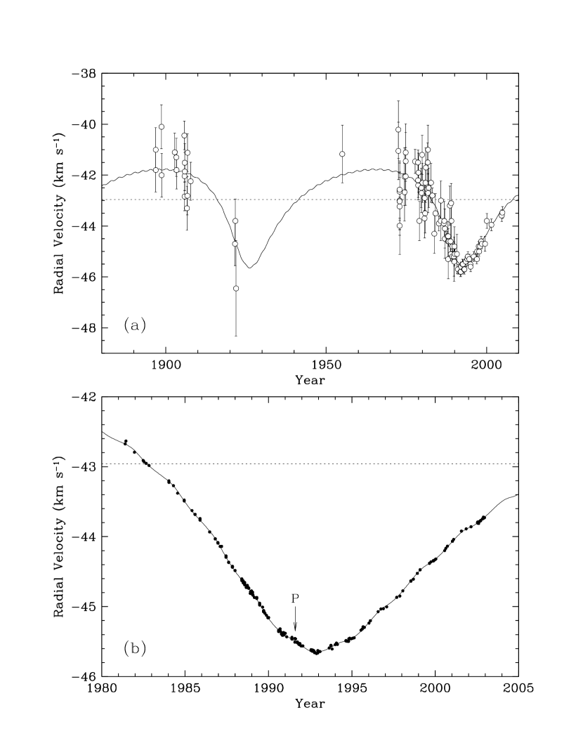
Figure 1.— Radial velocity measurements of $\gamma$ Cep A as a function of time, along with our fitted curve from the combined solution. The center-of-mass velocity of the system is indicated by the dotted line, and is on the reference frame of the velocities by Griffin, Carquillat & Ginestet (2002). (a) Classical velocity measurements in the outer orbit. The wiggles in the curve correspond to the perturbation by the 2.47-yr substellar companion. (b) Close-up of the high-precision velocities, which are near periastron passage in the outer orbit (arrow). The error bars in this panel are smaller than the size of the points.

Figure 2.— High-precision radial velocity measurements of $\gamma$ Cep shown as a function of phase in the inner orbit, along with our fitted curve from the combined solution. The motion in the outer orbit has been subtracted. The center-of-mass velocity of the system is indicated by the dotted line, and is on the reference frame of the velocities by Griffin, Carquillat & Ginestet (2002).

Figure 3.— Path of $\gamma$ Cep A on the sky resulting from the combined effects of proper motion, orbital motion ($P=66.8$ yr), and parallactic motion (solid curve). The magnitude and direction of the annual proper motion is indicated by the arrow. The Hipparcos observations are shown as dots at their predicted locations, and do not represent the actual measurements, which are one-dimensional in nature (see text). The dotted curve shows the path the star would follow in the absence of orbital motion, starting at the epoch of the first Hipparcos measurement, indicated with the open circle.

Figure 4.— Computed orbit of $\gamma$ Cep A around the center-of-mass of the binary (shown with a plus sign). The direction of motion (retrograde) is indicated by the arrow, and the dotted line represents the line of nodes. The Hipparcos observations are displayed with filled circles at their predicted locations, and are seen to bracket periastron passage (open circle labeled “P”). The perturbation due to the substellar companion of the primary is negligible on the scale of this figure. The relative orbit of the binary is simply a scaled-up version of the ellipse shown here, with a scale factor given by $(M_{\rm Aa}+M_{\rm B})/M_{\rm B}=4.26$ (yielding a semimajor axis $a^{\prime\prime}_{\rm AB}=1\farcs 382\pm 0\farcs 047$; see Table 3).

Figure 5.— Enlargement of Figure 4 showing the individual Hipparcos observations. See text for an explanation of the graphical representation of these one-dimensional measurements.

Figure 6.— Ground-based catalog positions of $\gamma$ Cep in Right Ascension and Declination, after subtracting the contribution from the proper motion resulting from our fit between the date of each observation and the reference epoch 1991.25. The curve represents the combination of motion in the 66.8-yr binary orbit and the parallactic motion, as predicted from the solution.

Figure 7.— Enlargement of Figure 6 showing only the most recent catalog measurements, which are the most precise.

Figure 8.— Constraint on the orbital period of the binary for two different data sets: the one in this paper (solid line), and the one used by Griffin, Carquillat & Ginestet (2002) (dashed line). In each case the period has been fixed over a fine grid of values and the remaining elements were solved for in the usual manner. The run of the reduced $\chi^{2}$ values for the present solution shows that of the two periods allowed by the Griffin, Carquillat & Ginestet (2002) fit, the 66-yr value is the correct one.

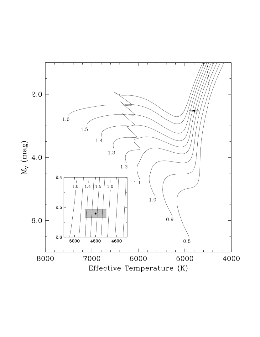
Figure 9.— Evolutionary tracks from the calculations by Yi et al. (2001) and Demarque et al. (2004) in the absolute visual magnitude vs. effective temperature plane. The metallicity adopted is [Fe/H] = +0.01, the weighted average of all spectroscopic determinations. Masses are labeled in solar units, and the dot with the shaded error box represents the measurements for $\gamma$ Cep. An enlargement is shown in the inset.

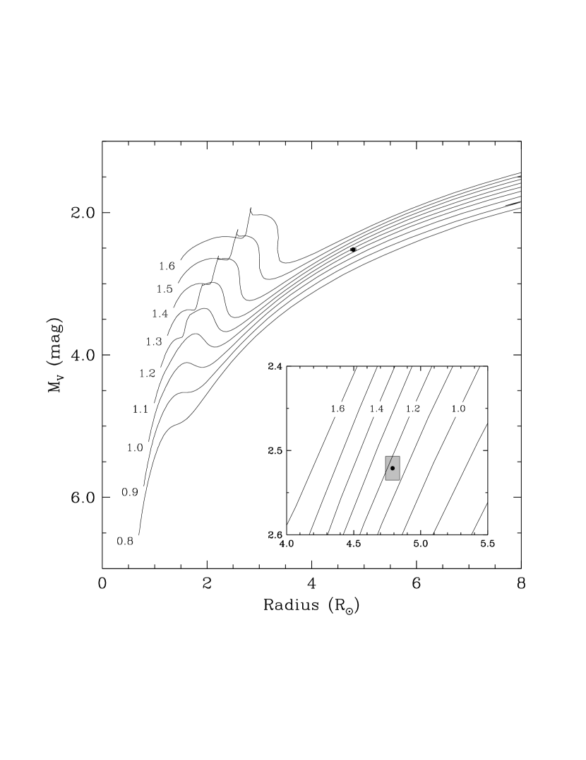
Figure 10.— Same as Figure 9 but in the $M_{V}$ vs. radius plane. The constraint on the mass of $\gamma$ Cep is seen to be much tighter.

Figure 11.— Theoretical mass and age combinations that are consistent with the four measured properties of $\gamma$ Cep ($T_{\rm eff}$, [Fe/H], $M_{V}$, and $R$) within their errors. The best fit is for $M_{\rm Aa}=1.18_{-0.11}^{+0.04}$ M_☉ and an age of $6.6_{-0.7}^{+2.6}$ Gyr. The larger point sizes indicate a closer match.

Figure 12.— Effective temperature and metallicity determinations for $\gamma$ Cep from only the studies that measured both quantities spectroscopically (filled circles). There is an apparent correlation between [Fe/H] and $T_{\rm eff}$. The values adopted in this paper are indicated with an asterisk. The arrows represent other spectroscopic abundance determinations that do not have a corresponding spectroscopic temperature measurement.

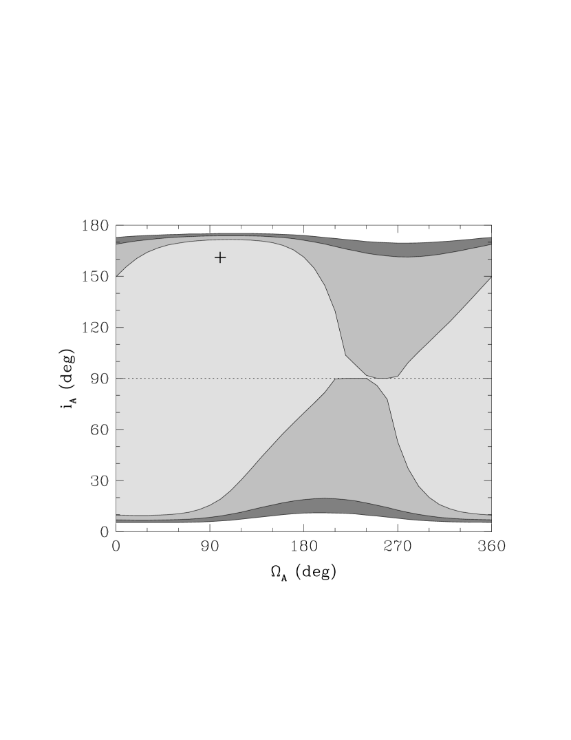
Figure 13.— Confidence levels of orbital fits in the $i_{\rm A}$–$\Omega_{\rm A}$ space of parameters, describing the wobble of $\gamma$ Cep A on the plane of the sky in response to the pull from the substellar companion. We use these fits to place an upper limit on the mass $M_{p}$ of the substellar companion. The light gray area represents solutions for fixed values of these two parameters that can be ruled out only at the $\sim$68% confidence level (1$\sigma$) or less. The plus sign corresponds to the best fit, which however does not give a statistically significant result (see text). The middle shade of gray corresponds to fits ruled out at confidence levels between 1$\sigma$ and 2$\sigma$, and yields an upper limit on $M_{p}$ of 13.3 M_Jup. The dark gray area corresponds to fits ruled out at confidence levels between 2$\sigma$ and 3$\sigma$. The outer edge of this region yields a minimum inclination angle of $4\fdg 9$, and an upper limit on $M_{p}$ of 16.9 M_Jup.

Appendix A Zero-point corrections to the radial velocities of $\gamma$ Cep from the literature

The historical sources containing radial velocity measurements of $\gamma$ Cep typically include other stars observed either as standards or for other purposes. The likelihood that many of those stars have been observed multiple times at the CfA is fairly high given that the spectroscopic database at CfA contains tens of thousands of stars and about a quarter of a million spectra to date. This common ground enables us to place the measurements of each of the sources on the CfA velocity system. In each case we selected all stars with no obvious signs of velocity variation that have been observed at least 3 times at the CfA. Radial velocities were derived from the available CfA spectra in the same way as those for $\gamma$ Cep, by cross-correlation using synthetic templates based on model atmospheres by R. L. Kurucz (see Nordström et al., 1994; Latham et al., 2002). The optimal template for each star was determined from grids of cross-correlations against a large number of synthetic spectra over broad ranges in the template parameters (mainly the effective temperature and rotational velocity), in the manner described by Torres, Neuhäuser & Guenther (2002). Solar metallicity was assumed throughout. Many of the stars are giants but there are some dwarfs as well, so the optimal surface gravity for the template in each case was determined by repeating the procedure above for a range of values of $\log g$, and selecting the one giving the highest correlation averaged over all exposures of the star. The radial velocities derived with these templates were then compared with those from each literature source.

Some of these sources have relatively few stars that can be used as standards, and rejecting objects that have not been observed at CfA leads to the loss of potentially useful comparison stars in some cases, which can compromise the determination of the offset. Those stars can still be used so long as they are included in another of the data sets, which then provides the link to the CfA system. Thus, instead of separately comparing each source with CfA to determine the corresponding velocity offset, as might commonly be done, we have followed a procedure by which we determine the velocity offsets of all sources simultaneously by minimizing the scatter of the velocities for all standard stars taken together. In this way any star that is included in at least two of the data sets (whether or not one of them is CfA) can be used to strengthen the solution. The quantity we seek to minimize is

$$\chi^{2}=\sum_{i=1}^{N_{\rm sets}}\sum_{j=1}^{N_{i,\rm stars}}\sum_{k=1}^{N_{ij,\rm obs}}\left({RV_{ijk}-\overline{RV_{j}}\over\sigma_{ijk}}\right)^{2}~{},$$ (A1)

where the sums are performed over all data sets ($i=1,\ldots,N_{\rm sets}$), all stars in each data set ($j=1,\ldots,N_{i,\rm star}$), and all observations of each star ($k=1,\ldots,N_{ij,\rm obs}$). The quantity $\sigma_{ijk}$ represents the uncertainty of each observation. The mean radial velocity for each star, $\overline{RV_{j}}$, is a function the adjustable parameters (offsets $\Delta_{i}$) given by

$$\overline{RV_{j}}=\sum_{i=1}^{N_{\rm sets}}\sum_{k=1}^{N_{ij,\rm obs}}\left(RV_{ijk}+\Delta_{i}\right)/\sum_{i=1}^{N_{\rm sets}}N_{ij,\rm obs}~{},$$ (A2)

and changes as the iterations proceed. Since the offsets are computed relative to CfA (defined here as the first data set), $\Delta_{1}\equiv 0$.

Table 6 presents the results for each data set from our least-squares solution. We list the derived offset along with its uncertainty, the number of standard stars in each group, the number of observations of $\gamma$ Cep, and the interval of those observations. With a few exceptions the total number of standard star observations used in each data set is typically a few dozen, while the overall number of CfA observations used for those same standards is $\sim$3300. The offsets were added with their corresponding sign to the individual velocities of $\gamma$ Cep in each data set to place them on the CfA system.

Table 6Radial velocity offsets applied to the literature sources containing measurements of $\gamma$ Cep, to bring them onto the CfA system.

	Offset $\Delta$	Standard	RVs for	Time span
Source	(km s-1)	stars	$\gamma$ Cep	(yr)
Frost & Adams (1903)	$-$1.33 $\pm$ 0.47	12	3	1902.8–1903.3
Bélopolsky (1904)	$-$0.48 $\pm$ 0.93	05	4	1903.7
Slipher (1905)	$-$0.97 $\pm$ 0.58	09	3	1905.8
Küstner (1908)	$-$1.38 $\pm$ 0.70	12	5	1905.9–1907.8
Abt (1973)	$+$0.46 $\pm$ 0.23	14	3	1916.0–1917.8
Harper (1934)	$+$1.82 $\pm$ 0.22	21	1	1921.9
Boulon (1957)	$-$1.50 $\pm$ 0.28	06	1	1955.0
Snowden & Young (2005)	$+$0.75 $\pm$ 0.16	14	130	1972.5–1974.7
Kjærgaard et al. (1981)	$+$0.11 $\pm$ 0.48	14	1	1977.7
CfA	+0.00	71	3	2001.5–2004.9

References

- Abt (1973) Abt, H. A. 1973, ApJS, 26, 365
- Affer et al. (2005) Affer, L., Micela, G., Morel, T., Sanz-Forcada, J., & Favata, F. 2005, A&A, 433, 647
- Allende Prieto & Lambert (1999) Allende Prieto, C., & Lambert, D. L. 1999, A&A, 352, 555
- Bakos (1971) Bakos, G. A. 1971, JRASC, 65, 222
- Baraffe et al. (1998) Baraffe, I., Chabrier, G., Allard, F., & Hauschildt, P. H. 1998, A&A, 337, 403
- Beavers & Eitter (1986) Beavers, W. I., & Eitter, J. J. 1986, ApJS, 62, 147
- Bélopolsky (1904) Bélopolsky, A. 1904, ApJ, 19, 85
- Bessell & Brett (1988) Bessell, M. S., & Brett, J. M. 1988, PASP, 100, 1134
- Boulon (1957) Boulon, J. 1957, J. des Obs., 40, 107
- Brown et al. (1989) Brown, J. A., Sneden, C., Lambert, D. L., & Dutchover, E. Jr. 1989, ApJS, 71, 293
- Campbell (1978) Campbell, R. 1978, AJ, 83, 1430
- Campbell & Moore (1928) Campbell, W. W., & Moore, J. H. 1928, Publ. Lick Obs., 16, 342
- Campbell & Walker (1979) Campbell, B., & Walker, G. A. H., 1979, PASP, 91, 540
- Campbell, Walker & Yang (1988) Campbell, B., Walker, G. A. H., & Yang, S. 1988, ApJ, 331, 902
- Carlsberg Meridian Catalogue (1989) Carlsberg Meridian Catalogue La Palma No. 4 1989, Copenhagen Univ. Obs., Royal Greenwich Obs., Real Inst. y Obs. de la Armada en San Fernando
- Cayrel de Strobel, Soubiran & Ralite (2001) Cayrel de Strobel, G., Soubiran, C., & Ralite, N. 2001, A&A, 373, 159
- Chabrier et al. (2005) Chabrier, G., Baraffe, I., Allard, F., & Hauschildt, P. H. 2005, in Resolved Stellar Populations, ASP Conf. Ser., eds. D. Valls-Gabaud & M. Chavez, in press
- Delfosse et al. (2000) Delfosse, X., Forveille, T., Ségransan, D., Beuzit, J.-L., Udry, S., Perrier, C., & Mayor, M. 2000, A&A, 364, 217
- Demarque et al. (2004) Demarque, P., Woo, J.-H., Kim, Y.-C., & Yi, S. K. 2004, ApJS, 155, 667
- de Medeiros & Mayor (1999) de Medeiros, J. R., & Mayor, M. 1999, A&AS, 139, 433
- Donahue (1993) Donahue, R. A. 1993, Ph.D. Thesis, New Mexico State University
- Dvorak et al. (2003) Dvorak, R., Pilat-Lohinger, E., Funk, B., & Freistetter, F. 2003, A&A, 398, L1
- ESA (1997) ESA 1997, The Hipparcos and Tycho Catalogues (ESA SP-1200; Noordwijk: ESA)
- Franchini et al. (2004) Franchini, M., Morossi, C., Di Marcantonio, P., Malagnini, M. L., Chavez, M., & Rodríguez-Merino, L. 2004, ApJ, 613, 312
- Frost & Adams (1903) Frost, E. B., & Adams, W. S. 1903, ApJ, 18, 237
- Fuhrmann (2004) Fuhrmann, K. 2004, AN, 325, 3
- Głȩbocki (1972) Głȩbocki, R. 1972, Acta Astr., 22, 141
- Gontcharov, Andronova & Titov (2000) Gontcharov, G. A., Andronova, A. A., & Titov, O. A. 2000, A&A, 355, 1164
- Gratton (1985) Gratton, R. G. 1985, A&A, 148, 105
- Gratton et al. (1982) Gratton, L., Gaudenzi, S., Rossi, C., & Gratton, R. G. 1982, MNRAS, 201, 807
- Gray et al. (2003) Gray, R. O., Corbally, C. J., Garrison, R. F., McFadden, M. T., & Robinson, P. E. 2003, AJ, 126, 2048
- Gray & Nagar (1985) Gray, D. F., & Nagar, P. 1985, ApJ, 298, 756
- Griffin, Carquillat & Ginestet (2002) Griffin, R. F., Carquillat, J.-M., & Ginestet, N. 2002, The Observatory, 122, 90