A Model-Independent Photometric Redshift Estimator for Type Ia Supernovae

Abstract

The use of type Ia supernovae (SNe Ia) as cosmological standard candles is fundamental in modern observational cosmology. In this letter, we derive a simple empirical photometric redshift estimator for SNe Ia using a training set of SNe Ia with multiband ($griz$) light-curves and spectroscopic redshifts obtained by the Supernova Legacy Survey (SNLS). This estimator is analytical and model-independent; it does not use spectral templates. We use all the available SNe Ia from SNLS with near maximum photometry in $griz$ (a total of 40 SNe Ia) to train and test our photometric redshift estimator. The difference between the estimated redshifts $z_{phot}$ and the spectroscopic redshifts $z_{spec}$, $(z_{phot}-z_{spec})/(1+z_{spec})$, has rms dispersions of 0.031 for 20 SNe Ia used in the training set, and 0.050 for 20 SNe Ia not used in the training set. The dispersion is of the same order of magnitude as the flux uncertainties at peak brightness for the SNe Ia. There are no outlyers.

This photometric redshift estimator should significantly enhance the ability of observers to accurately target high redshift SNe Ia for spectroscopy in ongoing surveys. It will also dramatically boost the cosmological impact of very large future supernova surveys, such as those planned for Advanced Liquid-mirror Probe for Astrophysics, Cosmology and Asteroids (ALPACA), and the Large Synoptic Survey Telescope (LSST).

1 Introduction

The use of type Ia supernovae (SNe Ia) as cosmological standard candles (Phillips, 1993; Riess, Press, & Kirshner, 1995; Wang et al., 2003) is fundamental in modern observational cosmology. Obtaining the spectroscopic redshifts of SNe Ia is the most costly aspect of supernova surveys.

The use of broadband photometry in multiple filters to estimate redshifts of galaxies has become well established (Weymann et al., 1999). There are two different approaches in estimating photometric redshifts of galaxies. In the empirical fitting method (Connolly et al., 1995; Wang, Bahcall, & Turner, 1998), a training set of galaxies with measured spectroscopic redshifts are used to derive analytical formulae relating the redshift to colors and magnitudes. In the template fitting technique (see for example, Puschell, Owen, & Laing (1982); Lanzetta, Yahil, & Fernandez-Soto (1996); Mobasher et al. (1996); Sawicki, Lin, & Yee (1997)), the observed colors are compared with the predictions of a set of galaxy SED templates.

The multiband photometry of SNe has been used to select SNe Ia candidates (Dahl n & Goobar, 2002; Riess et al., 2004; Johnson & Crotts, 2006). Strolger et al. (2004) used the template fitting method to estimate the photometric redshift of SN host galaxies.

Cohen et al. (2000) carried out a blind test of the predictions of Wang, Bahcall, & Turner (1998) for galaxies in the Hubble Deep Field North (HDF), and demonstrated that this technique is capable of reaching a precision of $\sigma[(z_{phot}-z_{spec})/(1+z_{spec})]=0.05$ for the majority of galaxies with $z<1.3$. In this paper, we modify and further develop the technique of Wang, Bahcall, & Turner (1998), to derive a simple and model-independent empirical photometric redshift estimator for SNe Ia. This work is made possible by the Supernova Legacy Survey (SNLS) First Year Data Release (Astier et al., 2006).

We present our method in Sec.2, and the results in Sec.3. Sec.4 contains a simple guide to the use of our photometric redshift estimator. We discuss and summarize in Sec.5.

2 The Method

We derive the empirical photometric redshift estimator for SNe Ia by using observables that reflect the properties of SNe Ia as calibrated standard candles.

If SNe Ia were perfect standard candles, the most important observable in estimating their redshifts is the peak brightness. Since the SNLS has the best sampled light-curves in the $i$ band, we use the $i$ band maximum flux. We use the fluxes in $grz$ at the epoch of $i$ maximum flux to make an effective K-correction to the $i$ flux. Our first estimate of redshift is given by

$$z_{phot}^{0}=c_{1}+c_{2}g_{f}+c_{3}r_{f}+c_{4}i_{f}+c_{5}z_{f}+c_{6}i_{f}^{2}$$ (1)

where $g_{f}=2.5\log(f_{g})$, $r_{f}=2.5\log(f_{r})$, $i_{f}=2.5\log(f_{i})$, and $z_{f}=2.5\log(f_{z})$, with $f_{g}$, $f_{r}$, $f_{i}$, $f_{z}$ are fluxes in ADU counts in $griz$ at the epoch of $i$ maximum flux.

Next, we calibrate each SN Ia in its estimated restframe. We define

$$\Delta i_{15}=2.5\log(f_{i}^{15d}/f_{i}),$$ (2)

where $f_{i}^{15d}$ is the $i$ band flux at 15 days after the $i$ flux maximum in the estimated restframe, corresponding to the epoch of $\Delta t^{15d}=15*(1+z_{phot}^{0})$ days after the epoch of $i$ flux maximum.

We now arrive at the final photometric redshift estimator

$$z_{phot}=c_{1}+c_{2}g_{f}+c_{3}r_{f}+c_{4}i_{f}+c_{5}z_{f}+c_{6}i_{f}^{2}+c_{7}\Delta i_{15}$$ (3)

The coefficients $c_{i}$ (i=1,2,…,7) are found by using a training set of SNe Ia with $griz$ light-curves and measured spectroscopic redshifts. We use the jackknife technique (Lupton, 1993) to estimate the bias-corrected mean and the covariance matrix of $c_{i}$.

3 Results

The Supernova Legacy Survey (SNLS) First Year Data Release (Astier et al., 2006) consists of the photometry and redshifts of 71 SNe Ia. Of these, only 40 have $griz$ light-curves with $gz$ photometry covering the epoch of the maximum flux in the $i$ band. For each of these SN Ia, we fit the fluxes in the $i$ band light-curve to an asymmetrically stretched Gaussian introduced by Wang (1999):

$$f=f_{0}\,\exp\left\{-\left[\frac{t-t_{peak}}{w(t-t_{start})^{q}}\right]^{2}\right\}.$$ (4)

All the SNe Ia we used are well fitted by this form in the regions of interest (not too close to the tails). This yields a smooth light curve without spurious features. The $i$ band maximum flux and its corresponding epoch are given by $f_{0}$ ($f_{i}=f_{0}$) and $t_{peak}$ respectively. The fluxes in $grz$ at the same epoch ($t_{peak}$), $f_{g}$, $f_{r}$, $f_{z}$ are obtained from the $grz$ light-curves using linear interpolation. We assume a floor of $f_{g}=200$ (about the size of the flux errors) for SNe Ia with $f_{g}<0$. Eq.(1) is then used to obtain a first estimate of the SN redshifts, which allows an estimate of $\Delta t^{15d}$. Eq.(4) then gives $f_{i}^{15d}$ needed for Eq.(2). Eq.(3) gives the final result for the estimated redshifts of the SNe Ia.

Fig.1 shows the photometric redshifts estimated using the estimator derived in this paper, compared to the measured spectroscopic redshifts. The upper panel shows the results for using all 40 SNe Ia in deriving the coefficients in Eq.(3). The rms dispersion in $(z_{phot}-z_{spec})/(1+z_{spec})$ is 0.036. Note that there are no outlyers. This demonstrates the tight correlation between the $griz$ fluxes and $\Delta i_{15}$ with redshifts. The lower panel shows the results for using only the set containing the most recently discovered 20 SNe Ia in deriving the coefficients in Eq.(3). These coefficients are then used to predict the redshifts of the other 20 SNe Ia. The rms dispersion in $(z_{phot}-z_{spec})/(1+z_{spec})$ is 0.031 for the 20 SNe Ia used in the training set, and 0.050 for 20 SNe Ia not used in the training set.

To avoid biases that arise from hand picking the SNe Ia used in the training set, we have kept the 40 SNe Ia from SNLS in the order of their discovery, then split them evenly in the middle into two subsets, and used these as the training set and testing set respectively for our photometric redshift estimator.

Note that the lowest redshift SN Ia in the SNLS $griz$ sample is at $z=0.263$. Thus this photometric redshift estimator is not calibrated for SNe Ia at $z<0.263$. It will be straightforward to modify and extend this estimator to lower redshifts, as larger uniform samples of SNe Ia covering a greater range of redshifts become available.

Peculiar or highly extincted SNe Ia can sometimes be mistaken as high redshift SNe Ia. Table 1 lists 5 peculiar and 2 highly extincted SNe Ia (all are nearby). It demonstrates that the photometric redshift estimator presented here generally yields accurate or negative estimated redshifts for peculiar and highly extincted SNe Ia. Thus it will not lead to contamination of the high $z$ sample by nearby peculiar and highly extincted SNe Ia.

Table 1: Behavior of the photometric redshift estimator for peculiar and highly extincted SNe Ia.

SN name	$z_{photo}$	characteristic	reference
SN2005hk	-0.14	peculiar	Phillips et al. (2006b)
SN2002cx	-0.12	peculiar	Li et al. (2003)
SN1999ac	-0.1	peculiar	Phillips et al. (2006a)
SN1999by	0.00	peculiar	Garnavich et al. (2004)
SN1997br	-0.01	peculiar	Li et al. (1999)
SN2006X	-0.01	highly extincted	Krisciunas (2006)
SN1997cy	-0.12	highly extincted	Germany et al. (2000)

4 A Recipe for Using the Photometric Redshift Estimator

We now give a practical guide to the use of our photometric redshift estimator, Eq.(3). The coefficients $c_{i}$ have been derived using 20 SNe Ia, and tested using another 20 SNe Ia [see Fig.1(b)]. The bias-corrected mean and standard deviations of $c_{i}$, computed using the jackknife technique, are given by

$$c_{1} = 6.122\pm 2.006$$

$$c_{2} = -0.06545\pm 0.04548$$

$$c_{3} = -0.03268\pm 0.08201$$

$$c_{4} = -0.8225\pm 0.4513$$

$$c_{5} = -0.06292\pm 0.08601$$

$$c_{6} = 0.03979\pm 0.02104$$

$$c_{7} = 0.04552\pm 0.04335$$ (5)

We give the covariance matrix of $c_{i}$ in Table 2.

Table 2: The covariance matrix of $c_{i}$.

0.4022E+01	0.3364E-02	0.6515E-01	-0.8817E+00	0.2031E-01	0.3988E-01	0.3912E-01
0.3364E-02	0.2068E-02	0.3714E-03	0.2112E-02	-0.2602E-02	-0.2421E-03	0.9723E-03
0.6515E-01	0.3714E-03	0.6726E-02	-0.1750E-01	0.1978E-03	0.4210E-03	0.1924E-03
-0.8817E+00	0.2112E-02	-0.1750E-01	0.2037E+00	-0.1203E-01	-0.9101E-02	-0.5894E-02
0.2031E-01	-0.2602E-02	0.1978E-03	-0.1203E-01	0.7398E-02	0.5995E-03	-0.1549E-02
0.3988E-01	-0.2421E-03	0.4210E-03	-0.9101E-02	0.5995E-03	0.4429E-03	0.2314E-03
0.3912E-01	0.9723E-03	0.1924E-03	-0.5894E-02	-0.1549E-02	0.2314E-03	0.1879E-02

Here are the steps one should follow in using our photometric redshift estimator: (1) Estimate the flux and epoch of the $i$ band maximum, $f_{i}$ and $t_{peak}$. (2) Estimate the fluxes in $grz$ at the same epoch, $f_{g}$, $f_{r}$, and $f_{z}$. (3) Use Eq.(3) with $c_{i}$ (i=1,2,…,6) given in Eq.(5) and $c_{7}=0$ to obtain a first estimate of $z_{phot}^{0}$. (4) Use $z_{phot}^{0}$ to estimate $\Delta t^{15d}=15*(1+z_{phot}^{0})$. (5) Estimate the $i$ band flux at $\Delta t^{15d}$ days after $t_{peak}$, $f_{i}^{15d}$, and compute $\Delta i_{15}=2.5\log(f_{i}^{15d}/f_{i})$. (6) Use Eq.(3) with $c_{i}$ (i=1,2,…,7) given in Eq.(5) to obtain $z_{phot}$. (7) Use the covariance matrix of $c_{i}$ given in Table 1 to compute the standard deviation of $z_{phot}$.

Note that the SNLS zeropoints should be used to convert $g_{f}$, $r_{f}$, $i_{f}$, $z_{f}$ in Eqs.(1) and (3) into magnitudes (Astier et al., 2006), and the appropriate conversions should be made if the available photometry is in $BVRI$ instead of $griz$ (Fukugita et al., 1996).

5 Discussion and Summary

We have derived a model-independent photometric redshift estimator, Eqs.(3) & (5), for SNe Ia that uses only multiband photometry near maximum light, and a training set of SNe Ia with multiband photometry and measured spectroscopic redshifts. This estimator is simple and analytical, thus is very easy to implement (see Sec.4).

The test of our photometric redshift estimator using SNe Ia not used in the training set demonstrates that this estimator is robust, and with an accuracy that is of the same order of magnitude as the photometric errors (see Fig.1(b)). The large uncertainties in the coefficients $c_{i}$ used in our photometric redshift estimator (see Eq.(5) are indicative of the relatively small sample (20 SNe Ia) used for the training set, as well as photometric errors. Eq.(5) also shows that the most key constraints on redshift comes from the $g$ and $i$ band photometry.

As the quality of data improves, we expect that our photometric redshift estimator can be further improved to provide more accurate redshift estimates. This photometric redshift estimator can be easily modified and trained to apply to SNe Ia photometry in any choices of multiple bands.

The measurement of spectroscopic redshifts of SNe is the most costly and constraining aspect of a supernova survey. Our results will allow observers to estimate the redshifts rather accurately based on near maximum light multiband photometry only (after obtaining spectroscopic redshifts for a modest training set), thus greatly increase the efficiency of supernova spectroscopy of high redshift candidates.

In order to model the systematic uncertainties of SNe Ia as standard candles, it is critical to obtain a very large number of SNe. Future supernova surveys can easily obtain the multiband photometry of a huge number of supernovae (Wang, 2000; Wang et al., 2004), for example, using the Advanced Liquid-mirror Probe for Astrophysics, Cosmology and Asteroids (ALPACA) , and the Large Synoptic Survey Telescope (LSST) . It will not be practical to obtain spectroscopic redshifts for all the SNe Ia found by such surveys. With the dense sampling and accurate multiband photometry expected for future supernova surveys, it will be possible to refine our photometric redshift estimator to the accuracies suitable for cosmology (Huterer et al., 2004). This will dramatically boost the cosmological impact of very large future supernova surveys.

Acknowledgements I am grateful to the SNLS team for releasing their data, including multi-band light-curves in flux units, and to Kevin Krisciunas for providing me with unpublished photometry on SN2006X. This work is supported in part by NSF CAREER grant AST-0094335.

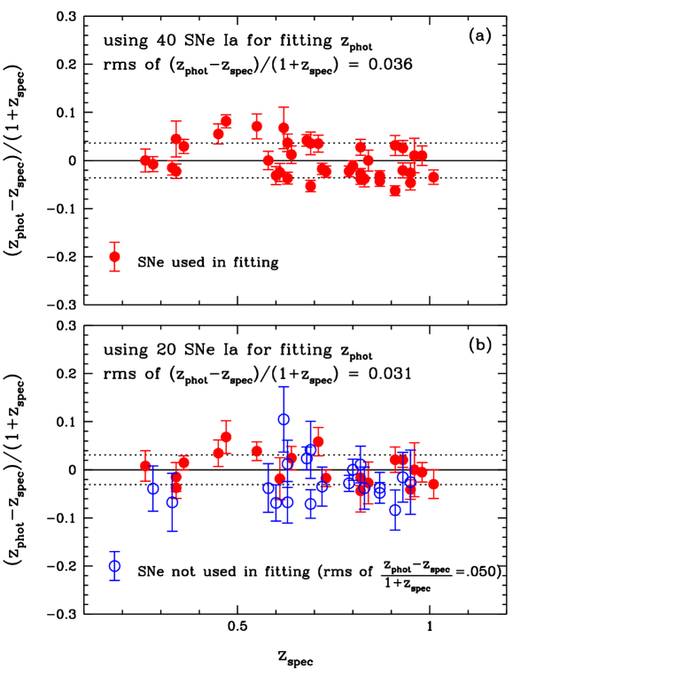
Figure 1: The photometric redshifts estimated using the estimator in Eq.(3), compared to the measured spectroscopic redshifts. (a) The results for using all 40 SNe Ia in deriving the coefficients in Eq.(3). (b) The results for using only the set containing the most recently discovered 20 SNe Ia in deriving the coefficients in Eq.(3). These coefficients are then used to predict the redshifts of the other 20 SNe Ia.

References

- Astier et al. (2006) Astier, P., et al. 2006, A & A 447, 31-48 (2006)
- Cohen et al. (2000) Cohen, J. G., et al. 2000, ApJ, 538, 29
- Connolly et al. (1995) Connolly, A. J., et al., 1995, AJ, 110, 2655
- Dahl n & Goobar (2002) Dahl n, T.; Goobar, A. 2002, PASP, 114, 284
- Fukugita et al. (1996) Fukugita, M., et al. 1996, AJ, 111, 1748
- Garnavich et al. (2004) Garnavich, P.M., et al. 2004, ApJ, 613, 1120
- Germany et al. (2000) Germany, L.M., et al. 2000, ApJ, 533, 320
- Huterer et al. (2004) Huterer, D., et al. 2004, ApJ, 615, 595
- Johnson & Crotts (2006) Johnson, B. D.; Crotts, A. P. S. 2006, AJ, 132, 756
- Lanzetta, Yahil, & Fernandez-Soto (1996) Lanzetta, K. M.; Yahil, A.; Fernandez-Soto, A. 1996, Nature, 381, 759
- Li et al. (1999) Li, W., et al. 1999, AJ, 117, 2709
- Li et al. (2003) Li, W., et al. 2003, PASP, 115, 453
- Lupton (1993) Lupton, R., 1993, “Statistics in Theory and Practice”, Princeton University Press
- Krisciunas (2006) Krisciunas, K., http://www.nd.edu/ kkrisciu/sn2006X.html
- Mobasher et al. (1996) Mobasher, B., et al. 1996, MNRAS, 282, L7
- Phillips (1993) Phillips, M.M. 1993, ApJ, 413, L105
- Phillips et al. (2006a) Phillips, M.M., et al. 2006a, astro-ph/0601684, AJ, in press
- Phillips et al. (2006b) Phillips, M.M., et al. 2006b, astro-ph/0611295
- Puschell, Owen, & Laing (1982) Puschell, J. J.; Owen, F. N.; Laing, R. A. 1982, ApJ, 257, L57
- Riess, Press, & Kirshner (1995) Riess, A.G., Press, W.H., and Kirshner, R.P. 1995, ApJ, 438, L17
- Riess et al. (2004) Riess, A. G., et al. 2004, ApJ, 607, 665
- Sawicki, Lin, & Yee (1997) Sawicki, M. J.; Lin, H.; Yee, H. K. C., 1997, AJ, 113, 1
- Strolger et al. (2004) Strolger, L., et al. 2004, ApJ, 613, 200
- Wang et al. (2003) Wang, L. et al., 2003, ApJ, 590, 944
- Wang (1999) Wang, Y. 1999, ApJ, 525, 651
- Wang (2000) Wang, Y. 2000, ApJ 531, 676
- Wang, Bahcall, & Turner (1998) Wang, Y.; Bahcall, N.; Turner, E. L., 1998, AJ, 116, 2081
- Wang et al. (2004) Wang, Y., et al. 2004 (the JEDI Collaboration), BAAS, v36, n5, 1560. See also http://jedi.nhn.ou.edu/.
- Weymann et al. (1999) Weymann, R.J.; Storrie-Lombardi, L.J.; Sawicki, M.; Brunner, R.J. 1999., Editors, “Photometric Redshifts and High Redshift Galaxies”, ASP Conference Series, Vol 191