A Probabilistic Approach to Classifying Supernovae Using Photometric Information

Abstract

This paper presents a novel method for determining the probability that a supernova candidate belongs to a known supernova type (such as Ia, Ibc, IIL, etc.), using its photometric information alone. It is validated with Monte Carlo, and both space- and ground- based data. We examine the application of the method to well-sampled as well as poorly sampled supernova light curves and investigate to what extent the best currently available supernova models can be used for typing supernova candidates. Central to the method is the assumption that a supernova candidate belongs to a group of objects that can be modeled; we therefore discuss possible ways of removing anomalous or less well understood events from the sample. This method is particularly advantageous for analyses where the purity of the supernova sample is of the essence, or for those where it is important to know the number of the supernova candidates of a certain type (e.g., in supernova rate studies).

1 Introduction

Type Ia supernovae, empirically established to be standardized candles, are a staple of experimental cosmology. A number of future cosmological probes (e.g., DES, Pan-STARRS, LSST, JDEM) are planning massive sky surveys that will collect very large samples of supernovae, which will have to be classified into several known types. Supernova candidates are most easily classified by their spectra, but for very large ground-based surveys it may be impractical to obtain a spectral confirmation of the supernova type for each candidate. Therefore, it is imperative to develop reliable methods of supernova classification based on photometric information alone. Photometric typing has been described in Poznanski et al. (2002), Riess et al. (2004a), Johnson and Crotts (2005) and  Sullivan et al. (2005), among others. Most of the existing methods rely on color-color or color-magnitude diagrams for supernova classification.

In this paper, we propose a novel approach to the photometric typing of supernova candidates. This method is based on a probability derived using a Bayesian approach, and is well suited for extracting the maximum amount of information out of limited data. Unlike methods relying on color-color or color-magnitude diagrams, which require a comparison of the candidate’s color(s) with pre-existing tables or plots – a comparison that requires a good understanding of the errors and assumptions that went into the making of the literature data – our approach calls for a calculation of a single number and automatically takes into account all of the information that is available for a given candidate while incorporating the currently best-known models for supernova behavior.

A Bayesian method in the context of supernova light curve fitting has been used in Barris and Tonry (2004); however, it was applied specifically to type Ia supernovae to deduce redshift-independent distance moduli. In this paper, on the other hand, we describe a probabilistic approach to typing photometrically surveyed supernovae. Such an approach allows the possibility of the marginalization (integration) of the unknown, or nuisance, parameters. In contrast to a traditional $\chi^{2}$ calculation, this technique is simply a calculation of a probability and does not involve fitting or minimization. However, it does require that the candidate sample be well understood; or, in other words, that each candidate be one of a number of hypothesized objects whose behavior can be well modeled.

The purpose of this paper is twofold. Apart from introducing a methodology that can be easily applied “as is” or extended as needed, we would like to test the extent to which applying the best currently available supernova models helps in typing supernova candidates. There is no doubt that within the next several years new and improved supernova models will be constructed; when they are, they can be easily worked into the method.

The paper is structured as follows. In Section 2, we derive the probability that a given candidate is a Type Ia supernova. In Section 3, we discuss how well the method works when applied to poorly sampled, Hubble Space Telescope GOODS data, and to well-sampled, ground-based SNLS data. We suggest further improvements to the method in Section 3.5, discuss its possible application to “anomalous” objects in Section 3.6; and to fitting for supernova parameters, in Section 3.7. Conclusions are given in Section 4.

2 The Probability

Let us suppose that we have a sample of supernova candidates where it has been established that every candidate is consistent with some type of astronomical object with known or well-modeled photometric behavior (one approach to making sure that this is indeed the case is discussed in Section 3.6). In our example, we consider photometric models for type Ibc IIL, IIP, IIn, and standard, or “Branch-normal” (Branch et al., 1993), type Ia supernovae because they are currently best known; however, the method can be trivially extended to include other supernova types, as well as variable objects that are not supernovae, once reliable models for such objects are available. We would like to determine the probability that a given candidate in the sample is a supernova of some known type $T$, given its measured light curve data. Here, we will focus on the case where $T$ is Ia, but the method can be easily applied to other types as well.

Here and for the remainder of the paper we assume that the redshift of the supernova candidate is perfectly known. We begin by assuming that the light curve of the candidate is measured in a single broadband filter $a$ (the method can be trivially extended to any number of filter bands). The light curve measurements are represented in $n_{epochs}$ (observing times) as $\{A_{i}\}$, where $i$ = [1,…,$n_{\rm epochs}$]. We would like to know the probability that this candidate is a type $T$ supernova, $P(T|\{A_{i}\})$. Technically, since $\{A_{i}\}$ defines the candidate, we are calculating the probability that the type $T$ hypothesis is true given a candidate, or:

$$P(T|\{A_{i}\})\equiv P(T|{\rm candidate}).$$ (1)

The probability $P(T|\{A_{i}\})$ depends on many parameters. We will express $P(T|\{A_{i}\})$ as a function of these parameters and, in the end, marginalize them to quantify $P(T|\{A_{i}\})$ .

Assume now that we have a photometric model (which we will also refer to as a template), $\{a_{j}\}$, for the expected light curve for a supernova of type $T$ at a given redshift, observed in filter $a$. In general, this model depends on parameters such as the date of maximum light $t_{0}$ (or, equivalently, the time difference between the dates of maximum light for the model and the data, $t_{\rm diff}$ ); stretch $s$ (Perlmutter et al, 1997), which parametrizes the width of the light curve (if $T$ = Ia); the assumed absolute magnitude $M$ in the restframe $B$-band; and interstellar extinction parametrized, e.g., by the Cardelli-Clayton-Mathis parameters $R_{v}$ and $A_{v}$ (Cardelli et al, 1998). We will refer to this collection of parameters as

$$\vec{\theta}\equiv(t_{\rm diff},s,M,R_{v},A_{v}).$$ (2)

The parameters $\vec{\theta}$ uniquely define $\{a_{j}\}$ for type $T$:

$$\{a_{j}\}\rightarrow\{a_{j}(\vec{\theta},T)\}$$ (3)

In this study, we would like to determine the probability $P({\rm Ia}|\{A_{i}\})$ that the candidate is a type Ia supernova given the measurements $\{A_{i}\}$. Unfortunately, this probability is not directly calculable, but one can easily calculate $P(\{A_{i}\}|{\rm Ia})$, the probability of obtaining the measurement given that the candidate is a type Ia supernova. Bayes’ theorem allows us to relate these two quantities. Naïvely, we may write

$$P({\rm Ia}|\{A_{i}\})=\frac{P(\{A_{i}\}|{\rm Ia})\,P({\rm Ia})}{\sum_{T}P(\{A_{i}\}|T)\,P(T)}$$ (4)

where $P(\{A_{i}\}|Ia)$ is the probability to obtain data $\{A_{i}\}$ for supernova type Ia, $P({\rm Ia})$ contains prior information about type Ia supernovae, and the denominator is the normalization over all of the known supernova types $T$. This sum is over a finite number of supernova types, which gives a legitimate probability because we assume that each candidate must be one of the types summed in the denominator. Of course, one would like the denominator to include a model for every possible object that could mimic or be a supernova; in practice, we have to limit ourselves to a subset of major supernova types with well-known photometric models.

When calculating $P({\rm Ia}|\{A_{i}\})$ one must consider that a range of possible values is allowed for the stretch, extinction, and other parameters that characterize a Type Ia supernova. Therefore, we express $P({\rm Ia}|\{A_{i}\})$ as a function of these parameters and then marginalize them:

$$P({\rm Ia}|\{A_{i}\})=\sum_{\vec{\theta}}\,P(\vec{\theta},{\rm Ia}|\{A_{i}\})$$

$$=\frac{\sum_{\vec{\theta}}\,P(\{A_{i}\}|\vec{\theta},{\rm Ia})P(\vec{\theta},{\rm Ia})}{\sum_{T}\,\sum_{\vec{\theta}}\,P(\{A_{i}\}|\vec{\theta},T)P(\vec{\theta},T)}.$$ (5)

The prior probability $P(\vec{\theta},T)$ contains all known information about the distributions of $t_{\rm diff}$, $M$, $s$, and other relevant parameters for type $T$ supernovae. Note that $P(\vec{\theta},T)$ could also include the relative probabilities of obtaining a type $T$ supernova, i.e., the relative rates of the different supernova types. However, in this study we will assume no prior knowledge of the relative supernova rates, and instead assume the rates are all the same.

Because $\vec{\theta}$ and $T$ uniquely define $\{a_{j}\}$, $P(\{A_{i}\}|\vec{\theta},T)$ can be written as:

$$P(\{A_{i}\}|\vec{\theta},T)\equiv P(\{A_{i}\}|\{a_{j}\}).$$ (6)

The measured light curve, $\{A_{i}\}$, is taken to be in units of counts/second, and can fluctuate from the model $\{a_{j}\}$ according to Gaussian statistics:

$$P(\{A_{i}\}|\vec{\theta},T)\equiv P(\{A_{i}\}|\{a_{j}\}=\prod_{i=1}^{n_{epochs}}\frac{e^{-\frac{(a_{j}-A_{i})^{2}}{2\delta A_{i}^{2}}}}{\sqrt{2\pi}\delta A_{i}}\Delta a_{j}.$$ (7)

In this expression, $A_{i}$ and $\delta A_{i}$ are experimental measurements and errors for epoch $i$, $\{a_{j}\}$ represents the predicted light curve for a type $T$ supernova, and $\Delta a_{j}$ is an increment of $a_{j}$.

We use the models (represented by $\{a_{j}\}$) for supernova Ia, Ibc, IIL, IIP, and IIn from Nugent (2006). Several issues are of the essence here. First, the model for type Ia supernovae extends both into the UV (below 3460 Å  in the supernova rest frame) and into the IR (above 6600 Å  in the supernova rest frame) regions. Both of these regions are poorly constrained with the currently available data. This is in fact the reason why some authors (Guy et al., 2005, for example) choose to limit themselves to only the well-known part of the type Ia supernova spectrum. Second, the behavior of non-type Ia supernovae, especially at high redshifts, is not well known; the currently available models may or may not be an adequate representation of these objects. In our work, however, we are interested in exploring the extent to which the best possible supernova models currently available offer a discriminating power. A Bayesian approach that allows one to easily work in the uncertainties on any prior knowledge of supernovae appears quite natural for the situation. The supernova models used in this work are discussed in more detail in Appendix A.

In order to calculate the prior $P(\vec{\theta}|T)$, we make the simplifying assumption that $R_{v}$ and $A_{v}$, $t_{\rm diff}$, $M$ and $s$ are all independent, allowing us to factorize the probability:

$$P(\vec{\theta}|T)=P(t_{\rm diff}|T)\,P(M|T)\,P(s|T)\,P(R_{v},A_{v}|T)\,P(T).$$ (8)

Let us consider each of the terms in Eqn. 8 in turn, starting with the probability $P(T)$ of observing a supernova of type $T$. Since we assume no prior knowledge of the relative rates of the various types, each type has an equal probability of appearing in the candidate sample. Therefore, $P(T)$ is a constant:

$$P(T)\equiv\frac{1}{N_{T}},$$ (9)

where $N_{T}$ is the number of supernova types considered.

We also assume a flat prior for the difference in the dates of maximum light between the model and the data, $t_{\rm diff}$. In practice, we compare the measured and modeled light curves shifting their relative dates of maximum by one day. Marginalization over $t_{\rm diff}$ thus means summing over a finite number of such shifts. As each shift has an equal probability and the prior must be normalized to 1,

$$P(t_{\rm diff}|T)\equiv\frac{1}{N_{\rm diff}}=\frac{\Delta t_{\rm diff}}{{t^{max}_{\rm diff}-t^{min}_{\rm diff}}}.$$ (10)

where $\Delta t_{\rm diff}$ is an increment of $t_{\rm diff}$, $N_{\rm diff}$ is the number of shifts, and the maximum $t^{max}_{\rm diff}$ and minimum $t^{min}_{\rm diff}$ set the limits on $t_{\rm diff}$. We take $N_{\rm diff}$ to be 160.

There are potentially large uncertainties associated with how well the luminosity function of a particular type supernova is known. This is accounted for in the prior $P(M|T)$:

$$P(M|T)=\frac{e^{-\frac{(M-\bar{M})^{2}}{2\delta M^{2}}}}{\sqrt{2\pi}\delta M}\Delta M.$$ (11)

Here, $\Delta M$ is an interval in $M$. We extract the mean magnitudes $\bar{M}$ in the restframe $B$-band from Nugent (2006), and the standard deviations, $\delta M$, from Richardson et al (2002). Table 1 summarizes the values used.

Supernova Type	$\bar{M}$	$\delta M$
Ia	-19.05	0.30
Ibc	-17.27	1.30
IIL	-17.77	0.90
IIP	-16.64	1.12
IIn	-19.05	0.92

Table 1: Mean magnitudes (Vega, restframe $B$-band) and standard deviations for different supernova types.

Note that there is an additional dispersion in magnitudes due to lensing effects; see, for example, Aldering et al (2006). We will ignore this effect in our study.

Concerning the prior on the stretch $s$, $P(s|T)$, we make a simplifying assumption that for type Ia supernovae the distribution for the stretch is the same for all filter bands. The concept of stretch itself, strictly speaking, is only defined in the restframe $B$- and $V$- bands, although an extension of the concept into the restframe $I$-band is discussed in Nobili et al (2005); an implementation of this extension would introduce several extra parameters into the likelihood calculation. For type Ia’s, the stretch is known to have a distribution given in Sullivan et al (2006). Approximating this distribution by a Gaussian:

$$P(s|{\rm Ia})=\frac{e^{-\frac{(s-\bar{s})^{2}}{2\delta s^{2}}}}{\sqrt{2\pi}\delta s}\Delta s,$$ (12)

where $\Delta s$ is an increment in $s$, and we obtain $\bar{s}$ = 0.97 and $\delta s$ = 0.09. For non-type Ia’s, the stretch is not defined. Practically speaking, this means that the light curves of non-type Ia candidates do not depend on the value of the stretch. We therefore assume a flat prior such that:

$$P(s|T)=\frac{1}{s_{max}-s_{min}}\Delta s\,\,\,({\rm for}~{}T\neq{\rm Ia})$$ (13)

where $s_{max}$ and $s_{min}$ can be arbitrary, provided they are consistent with the limits on the stretch considered for the type Ia case. Appendix B details why it is necessary to retain the stretch parameter for non-type Ia supernovae.

Lastly, we parametrize the effects of the interstellar extinction as in Cardelli et al (1998). The model supernova light curves are generated with some particular values of the Cardelli-Clayton-Mathis parameters $A_{v}$ and $R_{v}$. Introducing the actual distributions for $A_{v}$ and $R_{v}$ is difficult due to lack of a generally accepted model. For example, there have been several indications that the Milky Way value of $R_{v}$ = 3.1 may not be generally applicable. Values in the range of $\sim$2 to 3.5 have been suggested (Patil et al, 2006; Valencic et al, 2004). Likewise, there is no consensus for the distributions of $A_{v}$’s, although there do exist studies offering various non-analytic parametrization (for example, Hatano et al (1998) introduce a model of the extinction distribution as a function of the galaxy inclination, for both Ia and core-collapse supernovae). In our study, we compromise by considering a case of no extinction, as well as two cases of extinction with a moderate value of $A_{v}$ = 0.4 and two different values of $R_{v}$, 2.1 and 3.1. All three cases ($N_{v}=3$) are considered equally possible. In other words, we take:

$$P(R_{v},A_{v}|T)=\frac{1}{N_{v}},$$ (14)

where $N_{v}$ are the number of possible discrete values of $R_{v}$ and $A_{v}$ considered. It is worth noting that once more generally accepted models for $A_{v}$ and $R_{v}$ appear, it will be trivial to introduce them into the formalism.

We can now put everything together to calculate $\sum_{\vec{\theta}}\,P(\{A_{i}\}|\vec{\theta},T)P(\vec{\theta},T)$ for both Ia and non-Ia cases; for $T={\rm Ia}$:

$$\sum_{\vec{\theta}}\,P(\{A_{i}\}|\vec{\theta},{\rm Ia})P(\vec{\theta},{\rm Ia})=$$

$$\frac{1}{N_{T}}\sum_{t_{\rm diff}}\frac{1}{N_{t_{\rm diff}}}\sum_{R_{v},A_{v}}\frac{1}{N_{v}}\sum_{M=M_{min}}^{M_{max}}\frac{\Delta M}{\sqrt{2\pi}\delta M}\,e^{-\frac{(M-\bar{M})^{2}}{2\delta M^{2}}}\,\sum_{s=s_{min}}^{s_{max}}\frac{\Delta s}{\sqrt{2\pi}\delta s}\,e^{-\frac{(s-\bar{s})^{2}}{2\delta s^{2}}}$$

$$\prod_{i=1}^{n_{epochs}}\frac{\Delta a_{j}}{\sqrt{2\pi}\delta A_{i}}\,e^{-\frac{(a_{j}-A_{i})^{2}}{2\delta A_{i}^{2}}},$$ (15)

and for $T\neq{\rm Ia}$:

$$\sum_{\vec{\theta}}\,P(\{A_{i}\}|\vec{\theta},T)P(\vec{\theta},T)=$$

$$\frac{1}{N_{T}}\sum_{t_{\rm diff}}\frac{1}{N_{t_{\rm diff}}}\sum_{R_{v},A_{v}}\frac{1}{N_{v}}\sum_{M=M_{min}}^{M_{max}}\frac{\Delta M}{\sqrt{2\pi}\delta M}\,e^{-\frac{(M-\bar{M})^{2}}{2\delta M^{2}}}\,\sum_{s=s_{min}}^{s_{max}}\frac{\Delta s}{s_{max}-s_{min}}$$

$$\prod_{i=1}^{n_{epochs}}\frac{\Delta a_{j}}{\sqrt{2\pi}\delta A_{i}}\,e^{-\frac{(a_{j}-A_{i})^{2}}{2\delta A_{i}^{2}}}.$$ (16)

Finally, we can insert Eqns. (2) and (2) into (5) to obtain $P({\rm Ia}|\{A_{i}\})$. Naturally, if there are light curve measurements in more than one bandpass, the probability can be calculated for all of the available filters, each with its own photometric model dependent on the same parameters as in the single-filter case. For multi-filter measurements, there will be as many products over epochs in Eqns. (2) and (2) as there are passbands available.

Note that if the redshift of a supernova is not well known, it can also be introduced as a nuisance parameter. Likewise, the method can be trivially extended to include any other parameter of interest.

3 Demonstrating the Method

In order to demonstrate the method, we consider the following samples:

• Poorly sampled Hubble Space Telescope (HST) GOODS data consisting of both type Ia’s and non-Ia’s.

• Monte Carlo events with the same poor sampling as in the GOODS data.

• Well-sampled ground-based data consisting of all type Ia’s.

In all cases, we used the simulation described in Appendix A to create template light curves in the filter bands considered.

3.1 The Space-based GOODS Data

To illustrate how the method performs on space-based data when measurement epochs are scarce, we use the gold (“high confidence”) and silver (“likely but not certain”) candidates from the HST GOODS sample (Giavalisco et al, 2004; Dickinson et al, 2003; Renzini et al, 2001). The gold and silver classification is described in Riess et al (2004b), and refers to the level of confidence with which the type of a supernova was determined. The sample includes 15 gold and 5 silver Ia and 1 gold and 6 silver core-collapse (CC) candidates.

In addition to the GOODS data, we use a sample collected by the Supernova Cosmology Project (SCP) and the High-Z collaborations in the spring-summer of 2004. The latter sample covers the North GOODS field only and consists of 4 epochs separated by approximately 45 days. Because the data were recorded in only two filter passbands, HST ACS F775W and F850LP, in this section we will restrict ourselves to only using these two bands.

We start with the data that have been flat-fielded and gain-corrected by the HST pipeline, and use MultiDrizzle (Fruchter and Hook, 2002) to perform cosmic ray rejection and to combine dithered observations. We search for and perform simple aperture photometry on the supernova candidates in each of the five GOODS epochs. To obtain the multi-epoch photometry for the GOODS North data, we combine all four epochs of the SCP/High-Z sample and then subtract these data from each of the North GOODS epochs in turn. For the GOODS South data, we combine South epochs 4 and 5, as well as 1 and 2; we then subtract the two combined samples separately from each of the five South GOODS epochs.

We require that there be at least three data points with the signal-to-noise ratio S/N greater than 2, and that there be at least two data points with S/N greater than 3. This eliminates the “single-epoch” candidates 2003es, 2003eq, 2002lg, 2003ak, 2003eu, 2003al, and 2002fx (Ia’s), and 2003et and 2003er (CC’s). We also eliminate one silver Ia candidate, 2003lv, which appears to have a residual cosmic ray contamination. Figure 1 shows the probabilities $P({\rm Ia}|\{A_{i}\})$ for the remaining gold and silver candidates.

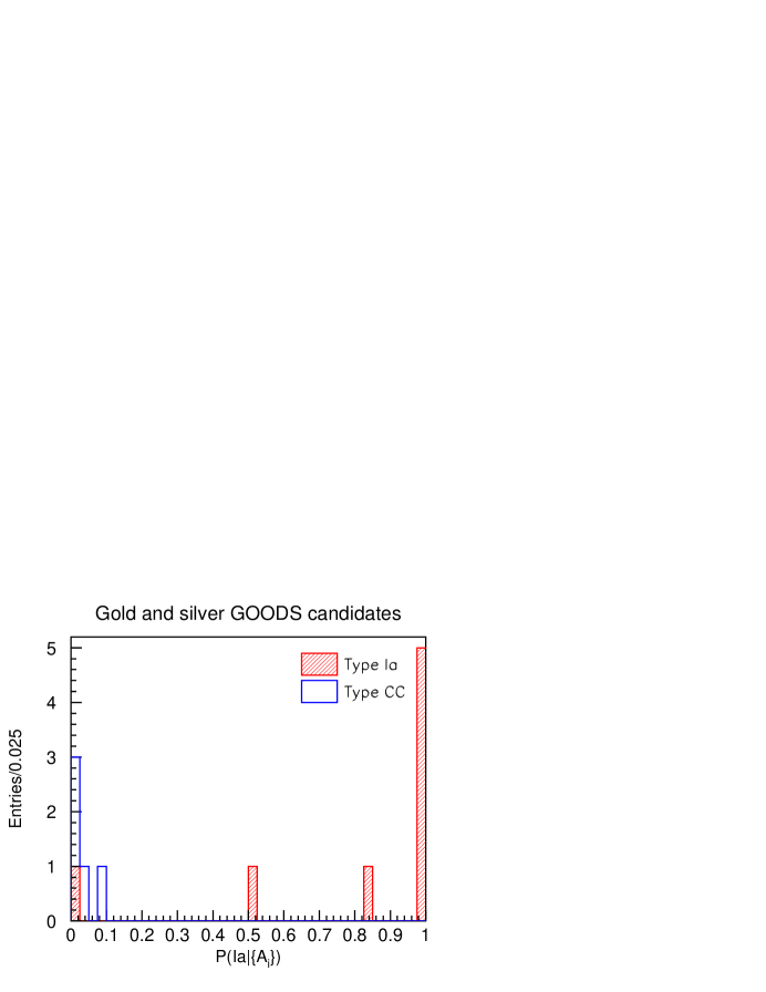
Figure 1: $P({\rm Ia}|\{A_{i}\})$ for the gold and silver GOODS candidates: Ia (red, hatched histograms) and CC (blue, empty histograms).

It is apparent that only one of the remaining type Ia candidates has a very low $P({\rm Ia}|\{A_{i}\})$. This candidate, 2003eb ($P({\rm Ia}|\{A_{i}\})$ = $2\times 10^{-4}$), appears to be more likely to be a type IIn than a type Ia. Note also that a silver Ia candidate, 2002fy, has a somewhat marginal $P({\rm Ia}|\{A_{i}\})$ of $\sim$0.52, because it appears about equally likely to be a Ia and a Ibc.

When discussing these results, it is important to be clear that we are not performing a fit but calculating a single probability, where we sum over many configurations with different stretches, magnitudes, etc. Nevertheless, it is useful to consider the one configuration that best matches the data, as this configuration will contribute the most to the final probability. Looking at these “best-matching” configurations is a good sanity check that the method is working. Figure 2 shows such best-matching configurations for two candidates, one Ia (2003bd) and one CC (2002kl). The best match for the former is a Ia model, while the best match for the latter is a Ibc model. It is apparent that the best matches describe the observed data well.

$\begin{array}[]{c@{\hspace{0.0in}}c}\includegraphics[width=216.81pt]{f2a.eps}&\includegraphics[width=216.81pt]{f2b.eps}\end{array}$

Figure 2: The best-matching configuration for a gold type Ia candidate (2003bd) (left plot) and for a silver type CC candidate (2002kl) (right plot). Solid lines are the templates for type Ia (left plot) and type Ibc (right plot) supernovae; filled circles with error bars are the data. The discontinuity of the templates in plot on the right is due to the fact that the available Ibc spectral template only extends to 85 days in the supernova rest frame past the supernova’s date of explosion.

3.2 Monte Carlo Simulations of the GOODS sample

It is encouraging to see that even though the data sampling for these space-based data is very poor, the method appears able to discriminate between different supernova types most of the time. In order to better understand the performance of the method on such data, we create Monte Carlo samples of all of the supernova types considered using the same sampling as that of the actual GOODS data (5 epochs separated by $\sim$45 days). We generate Monte Carlo samples of type Ia, Ibc, IIL, IIp, and IIn supernovae, each with 500 candidates whose redshifts, stretches, magnitudes, and extinction parameters are selected randomly according to the probability distributions in Eqns. (2) and (2). We simulate both ACS F850LP and F774W bands and impose the same signal-to-noise requirements on these simulated data as those we chose for the GOODS data, as described below.

Figure 3 shows the resulting probability distributions for identifying type Ia supernovae and, as an example of the usage of the method for identifying other types, type Ibc, IIL, IIP, and IIn supernovae. The near-zero probabilities for type $T$ supernovae in the $P(T|\{A_{i}\})$ plots come primarily from the events where the data populate the tails of the light curves and the discrimination between different types becomes particularly difficult. The uppermost right plot in Fig. 3 shows $P({\rm Ia}|\{A_{i}\})$ for the type Ia Monte Carlo sample as a function of redshift; it indicates that the lower probability events are also those with lower redshifts. This may simply be a consequence of the fact that our passbands of choice, F775W and F850LP, provide the best coverage for higher redshift candidates.

$\begin{array}[]{c@{\hspace{0.0in}}c}\includegraphics[width=180.67499pt]{f3a.eps}&\includegraphics[width=180.67499pt]{f3b.eps}\\ \includegraphics[width=180.67499pt]{f3c.eps}&\includegraphics[width=180.67499pt]{f3d.eps}\\ \includegraphics[width=180.67499pt]{f3e.eps}&\includegraphics[width=180.67499pt]{f3f.eps}\\ \end{array}$

Figure 3: All but uppermost right: $P(T|\{A_{i}\})$ for Monte Carlo generated events. The hatched histograms are for (from left to right, top to bottom): $T={\rm Ia}$, Ibc, IIL, IIP, and IIn, and the empty histograms are for all other types $T^{\prime}\neq T$. In all of the plots, the hatched and empty histograms are normalized to the area of the hatched histograms. The near-zero $P(T|\{A_{i}\})$ for type T come from the events where the data populate the tails of the light curves, making type discrimination difficult. The uppermost right plot shows $P({\rm Ia}|\{A_{i}\})$ for the Ia sample as a function of redshift. The box size is proportional to the number of events in the bin.

To select a sample of candidates of a given type, one would apply a cut, $p_{\rm cut}$, on $P(T|\{A_{i}\})$, such that $P(T|\{A_{i}\})$ $\geq$ $p_{\rm cut}$. The choice of the cut of course affects both the efficiency (defined as the fraction of type Ia candidates in a sample of Ia’s that passed the cut) and the purity (defined here as the fraction of non-type Ia candidates in a sample of non-Ia’s that passed the cut) of the sample. Using our Monte Carlo samples, we show both the efficiency of selecting type Ia’s and the degree of contamination of the sample with non-type Ia’s as a function of $p_{\rm cut}$ in Fig. 4 (left). It is apparent that the efficiency stays roughly flat, while the purity of the sample increases dramatically, with higher $p_{\rm cut}$. Figure 4 (right) shows the efficiency and purity distributions as a function of redshift for one choice of $p_{\rm cut}$, 0.95. Similarly to the tendency exhibited in Fig. 3(uppermost right), higher redshift candidates are both the most efficiency identified and suffer the greatest degree of contamination.

$\begin{array}[]{c@{\hspace{0.0in}}c}\includegraphics[width=180.67499pt]{f4a.eps}&\includegraphics[width=180.67499pt]{f4b.eps}\\ \end{array}$

Figure 4: Left plot: the efficiency for type Ia simulated supernovae (filled circles) and purity for non-type Ia simulated supernovae (filled triangles) as a function of the cut $p_{\rm cut}$ on $P(T|\{A_{i}\})$ (require that $P(T|\{A_{i}\})$ $\geq$ $p_{\rm cut}$). Right plot: the efficiency for type Ia simulated supernovae (filled circles) and purity for non-type Ia simulated supernovae (filled triangles) as a function of redshift for $p_{\rm cut}$ = 0.95.

It should be emphasized that demonstrating the method using Monte Carlo samples shows the behavior of $P(T|\{A_{i}\})$ in rather idealized circumstances; however, it can and should be used for studying the method’s performance.

3.3 The Ground-based Data

To demonstrate the method on well-sampled data, we use the Ia/Ia* candidates from the SNLS collaboration (Astier et al., 2006). Here, “Ia” denotes secure Ia’s; and “Ia*”, probable Ia’s, as defined in Howell et al. (2005). We generate the supernova templates in the four MegaCam bands where the data are available for most of the candidates: $g$, $r$, $i$, and $z$. Unlike the SALT fitter used by the SNLS collaboration (Guy et al., 2005), we do not restrict ourselves to a particular restframe wavelength range for creating the templates (the acceptable wavelength range considered in SALT ranges from 3460 Å  to 6600 Å). The supernova templates may well be rather unreliable outside the chosen SALT range, but we would like to find out to what extent they still offer type discrimination.

Figure 5 (left) shows the probabilities for the 73 SNLS Ia/Ia* candidates to be Ia’s, and Fig. 5 (right) shows an example of the best-matching configuration with respect to a type Ia model for one of the candidates, 03D4at.

$\begin{array}[]{c@{\hspace{0.0in}}c}\includegraphics[width=195.12877pt]{f5a.eps}&\includegraphics[width=195.12877pt]{f5b.eps}\end{array}$

Figure 5: Left plot: The probability distribution for Ia (hatched histogram) and Ia* (empty histogram) SNLS candidates. The plot does not show candidates 03D3bh, 03D4ag, and 04D3kr, which could not be identified as any known type (see Table 2). Right plot: The best-matching configuration for candidate 03D4at. Solid lines are the templates for a type Ia supernova; points with error bars are the data.

Out of the 73 SNLS Ia/Ia* candidates, one had a probability that was lower than 0.5 and three were “undefined” (i.e., they yielded zero $P(T|\{A_{i}\})$ for all supernova types $T$ considered). These four candidates are summarized in Table 2.

Candidate	Redshift	$P({\rm Ia}|\{A_{i}\})$	SALT $P(\chi^{2}|{\rm DOF})$	Comment
03D1gt	0.55	1.20e-9	0.86	No $g$-band SALT fit
03D3bh	0.25	undefined	3.64e-17	No $z$-band SALT fit
03D4ag	0.28	undefined	3.34e-27	No $z$-band SALT fit
04D3kr	0.34	undefined	0	No $z$-band SALT fit

Table 2: The four Ia/Ia* SNLS candidates that had low/undefined $P({\rm Ia}|\{A_{i}\})$. The candidates with undefined probabilities are those which had zero $P(T|\{A_{i}\})$ for all supernova types $T$ considered. Also listed are the $\chi^{2}$ probabilities given ${\rm DOF}$ degrees of freedom, $P(\chi^{2}|{\rm DOF})$, from the SALT fits. Note that for all of these candidates SALT did not fit one band ($g$ or $z$) as the mean wavelength corresponding to the omitted band in the supernova restframe was outside the acceptable SALT range of [3460 Å  - 6600 Å].

It should be noted that all four of these candidates had one band that was not fit by SALT, as the mean wavelength corresponding to the omitted band in the supernova restframe was outside the acceptable SALT wavelength range. Most other candidates in Fig. 5 (left) have a near-one $P({\rm Ia}|\{A_{i}\})$. Only one of them, 03D1fq, is somewhat of an outlier with a $P({\rm Ia}|\{A_{i}\})$ = 0.73. This candidate has data in only two out of the four bands, $i$ and $z$. The four failures and the fact that for all of them there was at least one band that was outside the [3460 Å  - 6600 Å] restframe range may well signal a failure of the template to provide an adequate description of the supernova behavior outside this range; however, the fact that only 4 out of 73 candidates failed to yield desired discrimination is encouraging.

It is also interesting to compare our probabilities $P(T|\{A_{i}\})$ with the results of the SALT fits – namely, the $\chi^{2}$ probabilities given ${\rm DOF}$ degrees of freedom, $P(\chi^{2}|{\rm DOF})$. Table 2 shows that the three “undefined” candidates also had exceptionally low $\chi^{2}$ probabilities from the SALT fits. Figure 6 (left) presents the $\chi^{2}$ probability of the SALT fits vs. $P({\rm Ia}|\{A_{i}\})$. One feature of this plot is the spread of the $\chi^{2}$ probabilities for the candidates for which we calculated $P({\rm Ia}|\{A_{i}\})$ to be essentially one.

$\begin{array}[]{c@{\hspace{0.0in}}c}\includegraphics[width=195.12877pt]{f6a.eps}&\includegraphics[width=195.12877pt]{f6b.eps}\end{array}$

Figure 6: Left: The SALT fits $P(\chi^{2}|{\rm DOF})$ probability vs. $P({\rm Ia}|\{A_{i}\})$ for the 70 SNLS Ia/Ia* candidates (the figure excludes the three candidates with undefined $P({\rm Ia}|\{A_{i}\})$ listed in Table 2). The box size is proportional to the number of events in the bin. Right: the efficiency of selecting type Ia supernovae for $p_{\rm cut}$ = 0.98 (we require $P({\rm Ia}|\{A_{i}\})$ $>$ $p_{\rm cut}$) as a function of redshift.

Figure 6 (right) shows the efficiency of selecting type Ia supernovae in the SNLS sample for one choice of $p_{\rm cut}$ = 0.98 (where we require $P({\rm Ia}|\{A_{i}\})$ to be greater than $p_{\rm cut}$), as a function of redshift. It is apparent that the efficiency remains flat within errors. We are unable to test the purity of this selection, as the non-type Ia candidates from the SNLS collaboration are not yet publicly available; however, we will certainly be able to do so when the data are released.

3.4 Systematic Effects

In order to investigate how changing the assumptions on the priors affects our results, we performed a number of simple tests. For all of the tests, we varied only one prior while keeping the rest of them unchanged.

• Assuming that the stretch parameter for all type Ia candidates is 1 increases the number of type Ia/Ia* SNLS candidates that have low ($<$ 0.5) or undefined $P({\rm Ia}|\{A_{i}\})$ from 4 to 6. It also lowers the probability for one gold Ia GOODS candidate, 2002hp, from 0.83 to 0.32; and for one silver Ia GOODS candidate, 2002fy, from 0.52 to 0.03.

• Assuming no extinction increases the number of SNLS candidates with low/undefined probabilities from 4 to 13. This change does not significantly alter the probabilities for the gold GOODS Ia candidates; however, it does lower $P({\rm Ia}|\{A_{i}\})$ for 2002fy to 0.15; and increases $P({\rm Ia}|\{A_{i}\})$ for one silver CC candidate, 2002kl, from 0.01 to 0.80.

• Using a flat prior on the magnitudes does not change the number of undefined probability SNLS candidates and moves candidate’s 03D1fq probability from 0.73 to 0.43. For the GOODS candidates, it lowers the probability for one silver Ia, 2002fy, from 0.52 to 0.14, but does not change the CC candidates’ probabilities.

• The assumption of the flat prior on the supernova rates is undoubtedly incorrect; however, it is difficult to suggest a plausible alternative since the rates for different supernova types (particularly for non-type Ias) are not well known, especially at high redshifts. Recent work (Dahlen et al., 2004, for example) seems to indicate that the rates of CC supernovae with respect to type Ia’s are higher by approximately a factor of 3 at redshifts up to $z$ $\sim$ 1. Assuming this ratio holds at all redshifts, and modifying the prior accordingly, 5 SNLS candidates end up with low or undefined probabilities. As far as GOODS candidates are concerned, this change lowers $P({\rm Ia}|\{A_{i}\})$ for 2002fy from 0.52 to 0.27; but does not alter the distribution for the CC candidates.

The choice of priors in any Bayesian method should be as complete as possible, reflecting the general belief about the relative probabilities of various choices of parameters. For the data we have considered, the choice of the extinction prior appears to have the biggest effect, although it is clear that all of the priors can have a dramatic effect on $P(Ia|\{A_{i}\})$ for some candidates. A change in any prior appears to be particularly consequential for the candidates whose classification was not strong to begin with (e.g., the starting $P({\rm Ia}|\{A_{i}\})$ with all of the default priors for the most affected gold Ia, 2002hp, was only about 0.83; and for the most affected silver Ia, 2002fy, it was 0.52).

3.5 Further Improvements

While the method described in the paper appears to be quite promising, there are a number of improvements that are still to be explored. For instance, we have ignored the correlations between supernova parameters by assuming the factorizable prior in Eqn. 8. Provided that these correlations are well known, they can be included in a Hessian matrix within the Gaussians. Another improvement would be to use the Poisson distributions in lieu of the Gaussians in Eqn. 7, especially for low photon statistics. In general, Poisson distributions have the added advantage of integrating nicely to Gamma functions under certain circumstances. Here, the photon rates are average counts over time, so they lend themselves better to Gaussian approximations. However, one could just as easily use absolute number of counts taken for a given epoch and use Poisson errors. Using better models, both for the supernova behavior and for the behavior of the parameters that affect supernova observations (e.g., the interstellar dust), is another issue that is important for providing a better discrimination. The proposed method is of course only as useful as the ability of the models it relies on to accurately represent the actual diversity of the observed supernova sample; future ground- and space- based samples will yield tremendous improvements in this regard.

3.6 Purging Anomalies

The calculation of $P({\rm Ia}|{\rm candidate})$ is highly dependent on characterizing the full range of objects that may be in the candidate sample. In practice, we must always consider the possibility that the candidate sample may be contaminated with “anomalies” that are merely mimicking a supernova signal – e.g., certain known variable astronomical types, such as AGNs, or residual “objects” resulting from poor image processing. Furthermore, while there are now spectral templates for many special supernova types (e.g., Ia 1991bg, 1991T, high velocity Ibc), there always exists the possibility that there are other, as of yet, undiscovered, supernova species. However, Eqns. 2 and 2 can be used to discard such anomalous supernovae with the following prescription.

First, we define a likelihood:

$$l(\vec{\theta},T|{\rm candidate})\,\equiv\,P(\{A_{i}\}|\vec{\theta},T)P(\vec{\theta},T)$$ (17)

so that

$$l(T|{\rm candidate})\,=\,\sum_{\vec{\theta}}\,l(\vec{\theta},T|{\rm candidate}).$$ (18)

Then, for each candidate, we calculate the likelihoods for the various types $T$, $l(T|{\rm candidate})$, as described above. We also generate large samples of Monte Carlo events for each type considered (Ia, Ibc, IIL, etc.), and calculate a corresponding likelihood distribution
$l(T|{\rm simulated~{}type~{}T~{}candidate})$ for each type $T$. We define parameter $Q$ such that if the probability of obtaining $l(T|{\rm simulated~{}type~{}T~{}candidate})$ $<$ $l(T|{\rm candidate})$ is smaller than $Q$, then the candidate is designated an anomaly. Effectively, $Q$ is the confidence level that the candidate is not a type $T$ supernova. Note that it is advantageous to consider each type $T$ in turn, rather than the entire denominator of Eqn. 5, since this approach does not force one to make any assumptions about the relative numbers of supernovae of type $T$ in the likelihood distributions.

The parameter $Q$ must be larger than the inverse of the number of simulated events for type $T$. In practice, the amount of CPU time limits the number of simulated supernovae that one can generate, and therefore constrains $Q$. Note that this method does not remove events whose light curves are similar to known types; $Q$ essentially defines how different the light curves of an anomaly must be from the known supernova light curves for it to be tagged an anomaly. Large values of $Q$ will possibly allow fewer anomalies that look similar to known supernova types to contaminate the “purified” sample, but will also decrease the statistics in the number of candidates of interest. A small $Q$ will require that anomalies differ more dramatically from the known supernova types, but it increases the statistics for the candidates that we want to measure. Small $Q$ values are also difficult to obtain as $Q$ is constrained by the number of simulations.

Using parameter $Q$ to make a cut on $l(T|{\rm candidate})$ is quite similar to using the more traditional $\chi^{2}$ analysis for candidate selection. The $\chi^{2}$ probability quantifies how likely it is that a measured distribution would have an equal or greater deviation from the model than the one observed. Likewise, we calculate the likelihood $l(T|{\rm candidate})$ and find how likely it is to for a particular candidate’s data to fluctuate to model $T$; if it is unlikely (i.e., the likelihood is less than $Q$) for all types, we call such a candidate an anomaly.

Note that this method would not effectively remove poorly sampled anomalies, as their probability would be relatively high for every type. The practicality of this approach for purging anomalies will be explored in a future paper.

Finally, note that using a method based on this simple likelihood criterion to provide the actual classification of supernovae is very different from our Bayesian classification approach, since it does not account for the possibility that a number of supernova types might have the same values for $\vec{\theta}$.

3.7 Fitting with the Maximum Likelihood

The Bayesian Adapted Template Match (BATM) method described in Barris and Tonry (2004) uses a maximum likelihood fit to extract supernova parameters. For completeness, we also describe the procedure for maximizing the likelihood for a given parameter, as well as for estimating the errors on the parameter.

The formulation of $l(\vec{\theta},T|{\rm candidate})$ lends itself to a maximum likelihood fit to $t_{\rm diff}$, $M$, $s$ or $R_{v}$ and $A_{v}$ provided that the supernova type $T$ is known. Indeed, we have maximized $l(\vec{\theta},T|{\rm candidate})$ to find the “best-matching” configurations of these variables in Section 3 (see Figs. 2 and 5(right plot)), where we see that it does an excellent job. However, these configurations were found by maximizing all the parameters at the same time. To find the best estimate for one parameter, we must assume the possibility that the others have some range of values - each with a corresponding probability. That is, we need only maximize one parameter at a time and marginalize the rest. In this scheme, errors are estimated by integrating the likelihood to obtain the upper and lower bound of the 68% confidence region.

For instance, suppose that we want the best estimate for the magnitude, $M$. We first marginalize all the parameters in the likelihood to obtain $l(M,T|{\rm candidate})$. Then, assuming that maximizing $l(M,T|{\rm candidate})$ gives the best estimate for the fitted parameters, we maximize $l(M,T|{\rm candidate})$ to obtain the best estimate for $M$, $M_{max}$. With the best estimate calculated, we then find the uncertainties by satisfying

$$0.16=\frac{\int_{0}^{M_{max}-\sigma_{M-}}l(M,T|{\rm candidate})dM}{\int_{0}^{\infty}l(M,T|{\rm candidate})dM}=\frac{\int_{M_{max}+\sigma_{M+}}^{\infty}l(M,T|{\rm candidate})dM}{\int_{0}^{\infty}l(M,T|{\rm candidate})dM}$$ (19)

where $M_{max}+\sigma_{M+}$ and $M_{max}-\sigma_{M-}$ are the upper and lower bounds of the $68\%$ confidence region. This procedure would then be repeated for all the parameters for which we want estimates, by maximizing $l(s,T|{\rm candidate})$, $l(t_{\rm diff},T|{\rm candidate})$, etc. Computationally, it may be necessary to replace the integrals with finite sums up to values where the terms of the likelihood are negligible, provided there is a single peak in the likelihood distribution.

Note that there are circumstances where maximizing $l(M,T|{\rm candidate})$ does not give the best estimate for the fitted parameters. As an example, Bhat et al. (1997) argue that a correction to the parameters is needed for this to be the case. This is one crucial reason why the performance of the likelihood always needs to be tested with Monte Carlo calculations.

4 Conclusion

We introduced a novel method to determine the probability that a supernova candidate is indeed a certain type of supernova sing photometric information alone. The probability is derived using a Bayesian approach. We have tested the method on both poorly sampled HST GOODS space-based data and well-populated SNLS ground-based light curves, with good results even for data where very few epochs available. While we considered primarily the application of this method to identifying type Ia supernova candidates, it can of course be used to identify any other known supernova types (see Fig. 3). The results of these studies show the method to be promising.

We have assumed that the candidate sample consists entirely of supernovae. The method naturally incorporates a number of possible hypotheses for the supernova types, allowing one to introduce prior knowledge of the probability distributions for various supernova parameters, as well as to marginalize them. Because it is crucial that the sample consist of candidates that have reliable models (i.e., well understood supernova types such as Branch-normal Ia, Ibc, etc.), we also proposed a possible approach for eliminating anomalous or less well understood candidates from the data. As more models for different supernova types become available, more candidates will pass this preliminary selection to be further considered for typing.

We have used the best currently available supernova models for all of the supernova types considered. While aware of their limitations, we note that using these models already yields good discriminating power; as better supernova models become available from the ongoing and upcoming ground- and space- based supernova surveys, classifying supernovae with this approach will become proportionally more reliable.

The method described in this paper could be useful for a number of studies. An obvious application is selecting a high-purity sample of type Ia’s for further analysis – e.g., creating a Hubble diagram and extracting cosmology. In order to do so, one would re-parametrize the likelihood in terms of the distance modulus $\mu$ and maximize $l(\mu,z,{\rm Ia}|{\rm candidate})$ to obtain the best estimates of the distance modulus and the redshift of the candidate, as well as the errors on these parameters, as described in Section 3.7. A pure sample of type $T$ supernovae could also be used for calculating the rates of this class of objects, provided one performs careful Monte Carlo studies of the method’s rejection factor for type $T$ supernovae. Another potentially useful application would be adapting the method for early-time light curve parameters in such a way as to make it a trigger for type Ia supernovae in large supernova surveys. Other possible extensions of the method would include introducing prior information on supernova rates for the different supernova types, as well as building a Bayes factor to measure the relative likelihood that a given candidate is more or less likely to be a Ia supernova than another type.

Appendix A Simulating Supernova Templates

In order to create the template supernova light curves in the available filter bands, we do the following. We start with a spectral template from Nugent (2006). The templates are made primarily from the publicly available supernova data assembled in the SUSPECT database. We consider five supernova types: Ibc, IIL, IIP, IIn, and Branch-normal Ia. The Branch-normal Ia template is based on Nugent (2002), with some additional features such as the smoothing out of the UV part. This template is for a stretch 1 Ia. The Ibc template is based on Levan et al. (2005); the IIL, IIP, and IIn templates are based on Gilliland et al. (1999), with a contribution from Baron et al. (2004) for IIP’s and from Di Carlo et al. (2002) for IIn’s.

Using the template for a given type, we compute the expected flux of the supernova at a given redshift, assuming the $\Lambda$CDM cosmology ($\Omega_{\Lambda}$ = 0.7, $\Omega_{M}$ = 0.3, and $w$ = const = -1). The templates are created for 12 different values of the peak $B$-band magnitudes, in the range of $\pm$ 3 $\delta M$, as listed in Table 1. For type Ia’s, each template is also generated for 14 different values of stretch, ranging from 0.6 to 1.3. Three types of templates are made: one assuming no interstellar extinction, and two with extinction parametrized by the Cardelli-Clayton-Mathis parameters $(A_{v},R_{v})$ = $(0.4,2.1)$ and $(0.4,3.1)$.

The simulation enables one to simulate either a ground- or a space- based observatory. The generated supernova flux is convolved with the atmospheric transmission (for the ground-based case), as well as relevant telescope, detector, and filter transmissions (for either ground- or space- based case). After the observations are thus generated, they are realized by an aperture exposure time calculator, creating light curves in each of the relevant filter bands. The signal-to-noise $S/N$ ratio is computed as:

$$\frac{S}{N}=\frac{R_{SN}\,f_{sig}\,t}{\sqrt{R_{SN}\,f_{sig}\,t+R_{sky}\,A\,t+R_{d}\,n_{p}\,t+N_{read}^{2}\,n_{p}\,n_{exp}+N_{\Delta}}}$$ (A1)

where $R_{SN}$ is the supernova source rate, $f_{sig}$ is the fraction of the source flux in the aperture, $t$ is the exposure time, $R_{sky}$ is the sky rate, $A$ is the effective seeing area, (computed taking into account the atmospheric seeing for the ground-based case, the diffraction radius calculated for a given filter central wavelength, the detector diffusion, and the detector pixel size), $R_{d}$ is the detector dark current rate, $N_{read}$ is the detector read noise, $n_{p}$ is the number of pixels in the aperture, $n_{exp}$ is the number of exposures, and $N_{\Delta}$ is the flatfielding contribution from the detector inter-pixel sensitivity variations:

$$N_{\Delta}=\left((f_{sig}\,R_{SN}+R_{sky}\,A+R_{d}\,n_{p})\times t\,\Delta\right)^{2}$$ (A2)

where $\Delta$ is the flatfielding error, taken to be 10^-4.

Appendix B The Stretch Parameter and Non-type Ia Supernovae

The stretch parameter is not defined for non-type Ia supernovae. However, the calculation of $P(T|{\rm candidate})$ necessitates that it be formally introduced for all candidates, regardless of type. If it was not included, the sum over the stretch in the numerator and denominator of Eqn. 5 would weight the non-type Ia’s by a factor of $s_{max}-s_{min}$.

To show how the stretch might be introduced for non-type Ia supernovae, we define $T^{\prime}$ as some generic non-type Ia supernova type, and

$$\vec{\theta}^{\prime}\equiv(t_{diff},M,A_{v},R_{v}).$$ (B1)

we then calculate $\sum_{\vec{\theta}}P(\{A_{i}\}|\vec{\theta}^{\prime},T^{\prime})P(\vec{\theta}^{\prime},T^{\prime})$ imposing Eqn. 8:

$$\sum_{\vec{\theta}}P(\{A_{i}\}|\vec{\theta},T^{\prime})P(\vec{\theta},T^{\prime})=\sum_{\vec{\theta}^{\prime}}\sum_{-\infty}^{\infty}P(\{A_{i}\}|\vec{\theta}^{\prime},s,T^{\prime})P(\vec{\theta}^{\prime},s,T^{\prime})$$ (B2)

$$=\sum_{\vec{\theta}^{\prime}}\sum_{-\infty}^{\infty}P(\{A_{i}\}|\vec{\theta}^{\prime},s,T^{\prime})P(\vec{\theta}^{\prime}|T^{\prime})P(s|T^{\prime})P(T^{\prime}).$$

where, not specifying anything about the stretch parameter $s$, we allow it to take on any value between $-\infty$ and $+\infty$.

Then, for type $T^{\prime}$ supernovae, we require that the likelihood, $P(\{A_{i}\}|\vec{\theta}^{\prime},s,T^{\prime})$ remain unchanged for any choice of $s$. That is,

$$P(\{A_{i}\}|\vec{\theta}^{\prime},s,T^{\prime})=P(\{A_{i}\}|\vec{\theta}^{\prime},T^{\prime}).$$ (B3)

Therefore, Eqn. B becomes

$$\sum_{\vec{\theta}^{\prime}}\sum_{-\infty}^{\infty}P(\{A_{i}\}|\vec{\theta}^{\prime},s,T^{\prime})P(\vec{\theta}^{\prime}|T^{\prime})P(s|T^{\prime})P(T^{\prime})$$ (B4)

$$=\sum_{\vec{\theta}^{\prime}}P(\{A_{i}\}|\vec{\theta}^{\prime},T^{\prime})P(\vec{\theta}^{\prime}|T^{\prime})P(T^{\prime})\sum_{-\infty}^{\infty}P(s|T^{\prime}).$$

If $p(s|T^{\prime})$ is the probability density such that $P(s|T^{\prime})=p(s|T^{\prime})\Delta s$, then probability theory requires

$$\sum_{-\infty}^{\infty}p(s|T^{\prime})\Delta s=1.$$ (B5)

However, Eqn. 5 remains the same if we set

$$p(s|T^{\prime})=\frac{1}{s_{max}-s_{min}};$$ (B6)

as well as replace the upper and lower bounds in Eqn. B5 with $s_{max}$ and $s_{min}$, respectively; and use the same limits of integration, $s_{min}$ and $s_{max}$, for both the numerator and denominator. This is the reason for the choice of stretch prior in Eqn. 13.

References

- Aldering et al (2006) G. Aldering et al., preprint astro-ph/0607030 (2006)
- Astier et al. (2006) P. Astier et al., A&A. 447, 31 (2006)
- Baron et al. (2004) E. Baron et al., ApJ 616, 91 (2004)
- Barris and Tonry (2004) B. J. Barris and J. L. Tonry, ApJ 613, L21 (2004)
- Bhat et al. (1997) P. Bhat, H. Prosper, and S. Snyder, Phys. Lett. B 407, 73, (1997)
- Branch et al. (1993) D. Branch, A. Fisher, P. Nugent, AJ 106, 2383 (1993)
- Cardelli et al (1998) J. A. Cardelli, G. C. Clayton, and J. S. Mathis, ApJ 329, L33 (1988)
- Dahlen et al. (2004) T. Dahlen et al., ApJ 613, 189 (2004)
- Di Carlo et al. (2002) E. Di Carlo et al, ApJ 573, 144 (2002).
- Dickinson et al (2003) M. Dickinson et al., in the proceedings of the ESO/USM Workshop “The mass of Galaxies at Low and High Redshift” (Venice, Italy, October 2001), eds. R. Bender and A. Renzini (2003)
- Fruchter and Hook (2002) A. Fruchter and R. N. Hook, PASP 114, 144 (2002)
- Giavalisco et al (2004) M. Giavalisco et al., ApJ 600, L93 (2004)
- Gilliland et al. (1999) R. L. Gilliland, P. E. Nugent, M. M. Phillips, ApJ 521, 30 (1999)
- Guy et al. (2005) J. Guy et al., accepted for publication in A&A, preprint astro-ph/0506583 (2005)
- Hatano et al (1998) K. Hatano, D. Branch, and J. Deaton, ApJ 502, 177 (1998)
- Howell et al. (2005) D. A. Howell et al., to be published in ApJ, (2005)
- Johnson and Crotts (2005) B. Johnson and A. Crotts, submitted to AJ, preprint astro-ph/0511377 (2005)
- Levan et al. (2005) A. Levan et al., ApJ 624 880 (2005)
- Nobili et al (2005) S. Nobili et al., A&A, 437, 789 (2005)
- Nugent (2006) P. E. Nugent, http://supernova.lbl.gov/nugent/nugent_templates.html (2006)
- Nugent (2002) P. E. Nugent, A. Kim, and S. Perlmutter, PASP 114, 803 (2002)
- Patil et al (2006) M. K. Patil, S. K. Pandey, D. K. Sahu, A. K. Kembhavi, accepted for publication in A$A, preprint astro-ph/0611369
- Perlmutter et al (1997) S. Perlmutter et al., ApJ 483, 565 (1997)
- Poznanski et al. (2002) D. Poznanski et al., PASP, 114, 833 (2002)
- Renzini et al (2001) A. Renzini et al., in the proceedings of the ESO/USM Workshop “The mass of Galaxies at Low and High Redshift” (Venice, Italy, October 2001), eds. R. Bender and A. Renzini (2003)
- Richardson et al (2002) D. Richardson et al., AJ 123, 745 (2002)
- Riess et al. (2004a) A. G. Riess et al., ApJ 600, L163 (2004a)
- Riess et al (2004b) A. G. Riess et al., ApJ 607, 665-687 (2004b)
- Sullivan et al. (2005) M. Sullivan et al., accepted for publication in AJ, preprint astro-ph/0510857 (2006)
- Sullivan et al (2006) M. Sullivan et al., accepted for publication in ApJ, preprint astro-ph/0605455 (2006)
- Valencic et al (2004) L. A. Valencic, G. C. Clayton, K D. Gordon, ApJ 616, 912 (2004)