The high redshift galaxy population in hierarchical galaxy formation models

Abstract

We compare observations of the high redshift galaxy population to the predictions of the galaxy formation model of Croton et al. (2006) and De Lucia & Blaizot (2006). This model, implemented on the Millennium Simulation of the concordance $\Lambda$CDM cosmogony, introduces “radio mode” feedback from the central galaxies of groups and clusters in order to obtain quantitative agreement with the luminosity, colour, morphology and clustering properties of the present-day galaxy population. Here we construct deep light cone surveys in order to compare model predictions to the observed counts and redshift distributions of distant galaxies, as well as to their inferred luminosity and mass functions out to redshift 5. With the exception of the mass functions, all these properties are sensitive to modelling of dust obscuration. A simple but plausible treatment agrees moderately well with most of the data. The predicted abundance of relatively massive ($\sim M_{*}$) galaxies appears systematically high at high redshift, suggesting that such galaxies assemble earlier in this model than in the real Universe. An independent galaxy formation model implemented on the same simulation matches the observed mass functions slightly better, so the discrepancy probably reflects incomplete galaxy formation physics rather than problems with the underlying cosmogony.

1 Introduction

Recent work has used the very large Millennium Simulation to follow the evolution of the galaxy population throughout a large volume of the concordance $\Lambda$CDM cosmogony (Springel et al., 2005; Croton et al., 2006; Bower et al., 2006; De Lucia et al., 2006; De Lucia & Blaizot, 2006). By implementing “semi-analytic” treatments of baryonic processes on the stored merger trees of all halos and subhalos, the formation and evolution of about $10^{7}$ galaxies can be simulated in some detail. The inclusion of “radio mode” feedback from the central galaxies in groups and clusters allowed these authors to obtain good fits to the local galaxy population and to cure several problems which had plagued earlier galaxy formation modelling of this type. In particular, they were able to produce galaxy luminosity functions with the observed exponential cutoff, dominated at bright magnitudes by passively evolving, predominantly elliptical galaxies. At the same time, this new ingredient provided an energetically plausible explanation for the failure of “cooling flows” to produce extremely massive galaxies in cluster cores. Most of this work compared model predictions to the systematic properties and clustering of the observed low redshift galaxy population, or studied the predicted formation paths of massive galaxies. Only Bower et al. (2006) compared their model in detail to some of the currently available data at high redshift. In the present paper we compare these same data and others to the galaxy formation model of Croton et al. (2006) as updated by De Lucia & Blaizot (2006) and made publicly available through the Millennium Simulation data site.

Many recent observational studies have emphasised their detection of substantial populations of massive galaxies out to at least redshift 2 and have seen this as conflicting with expectations from hierarchical formation models in the $\Lambda$CDM cosmogony (e.g. Cimatti et al., 2002b; Im et al., 2002; Pozzetti et al., 2003; Kashikawa et al., 2003; Chen et al., 2003; Somerville et al., 2004). This notion reflects in part the fact that early hierarchical models assumed an Einstein-de-Sitter cosmogony in which recent evolution is stronger than for $\Lambda$CDM (e.g. Fontana et al., 1999), in part an underassessment of the predictions of the contrasting toy model in which massive galaxies assemble at high redshift and thereafter evolve in luminosity alone (see Kitzbichler & White, 2006). Bower et al. (2006) find their model to be in good agreement with current observational estimates of the abundance of massive galaxies at high redshift, while our comparisons below suggest that the model of Croton et al. (2006) and De Lucia & Blaizot (2006) appears, if anything, to overpredict this abundance. As shown by these authors and particularly by De Lucia et al. (2006) both models predict “anti-hierarchical” behaviour, in that star formation completes earlier in more massive galaxies. This behaviour clearly does not conflict with the underlying hierarchical growth of structure in a $\Lambda$CDM cosmogony.

The current paper is organised as follows. In Section 2 we briefly describe the Millennium Simulation and the fiducial galaxy formation model we are adopting. Where we have made modifications, most significantly in the dust treatment, these are described in detail. We also give a detailed account of how we construct mock catalogues of galaxies along the backward lightcone of a particular simulated field of observation. Many of our methods resemble those which Blaizot et al. (2005) implemented in their MOMAF facility in order to enable mock observations of simulated galaxy catalogues of the same type as (though smaller than) the Millennium Run catalogues we use here. Our results are summarised in Section 3 where we compare number counts as a function of apparent magnitude and redshift with the currently available observational data. We also compare the predicted evolution of the luminosity and stellar mass functions to results derived from recent observational surveys, and we illustrate how the population of galaxies is predicted to shift in the colour-absolute magnitude plane. Finally in Section 4 we interpret our findings and present our conclusions.

2 The Model

2.1 The Millennium dark matter simulation

We make use of the Millennium Run, a very large simulation which follows the hierarchical growth of dark matter structures from redshift $z=127$ to the present. The simulation assumes the concordance $\Lambda$CDM cosmology and follows the trajectories of $2160^{3}\simeq 1.0078\times 10^{10}$ particles in a periodic box 500 Mpc/$h$ on a side. A full description is given by Springel et al. (2005); here we summarise the main simulation characteristics as follows:

The adopted cosmological parameter values are consistent with a combined analysis of the 2dFGRS (Colless et al., 2001) and the first-year WMAP data (Spergel et al., 2003; Seljak et al., 2005). Specifically, the simulation takes $\Omega_{\rm m}=\Omega_{\rm dm}+\Omega_{\rm b}=0.25$, $\Omega_{\rm b}=0.045$, $h=0.73$, $\Omega_{\Lambda}=0.75$, $n=1$, and $\sigma_{8}=0.9$ where all parameters are defined in the standard way. The adopted particle number and simulation volume imply a particle mass of $8.6\times 10^{8}\,h^{-1}{\rm M}_{\odot}$. This mass resolution is sufficient to resolve the haloes hosting galaxies as faint as $0.1\,L_{\star}$ with at least $\sim 100$ particles. The initial conditions at $z\!=\!127$ were created by displacing particles from a homogeneous, ‘glass-like’ distribution using a Gaussian random field with the $\Lambda$CDM linear power spectrum.

In order to perform such a large simulation on the available hardware, a special version of the GADGET-2 code (Springel et al., 2001b; Springel, 2005) was created with very low memory consumption. The computational algorithm combines a hierarchical multipole expansion, or ‘tree’ method (Barnes & Hut, 1986), with a Fourier transform particle-mesh method (Hockney & Eastwood, 1981). The short-range gravitational force law is softened on comoving scale $5\,h^{-1}{\rm kpc}$ which may be taken as the spatial resolution limit of the calculation, thus achieving a dynamic range of $10^{5}$ in 3D. Data from the simulation were stored at 63 epochs spaced approximately logarithmically in time at early times and approximately linearly in time at late times (with $\Delta t\sim 300$Myr). Post-processing software identified all resolved dark haloes and their subhaloes in each of these outputs and then linked them together between neighboring outputs to construct a detailed formation tree for every object present at the final time. Galaxy formation modelling is then carried out in post-processing on this stored data structure.

2.2 The basic semi-analytic model

Our semi-analytic model is that of Croton et al. (2006) as updated by De Lucia & Blaizot (2006) and made public on the Millenium Simulation data download site (see Lemson et al., 2006). These models include the physical processes and modelling techniques originally introduced by White & Frenk (1991); Kauffmann et al. (1993); Kauffmann & Charlot (1998); Kauffmann et al. (1999); Kauffmann & Haehnelt (2000); Springel et al. (2001a) and De Lucia et al. (2004), principally gas cooling, star formation, chemical and hydrodynamic feedback from supernovae, stellar population synthesis modelling of photometric evolution and growth of supermassive black holes by accretion and merging. They also include a treatment (based on that of Kravtsov et al., 2004) of the suppression of infall onto dwarf galaxies as consequence of reionisation heating. More importantly, they include an entirely new treatment of “radio mode” feedback from galaxies at the centres of groups and clusters containing a static hot gas atmosphere. The equations specifying the various aspects of the model and the specific parameter choices made are listed in Croton et al. (2006) and De Lucia & Blaizot (2006). The only change made here is in the dust model as described in the next section.

2.3 Improved dust treatment for the fiducial model

Even at low redshifts, a crucial ingredient in estimating appropriate magnitudes for model galaxies, particularly in the $B$-band, is the dust model. For the present-day luminosity function (LF) a simple phenomenological treatment calibrated using observations in the local universe has traditionally given satisfactory results (Kauffmann et al., 1999). However, the situation at high redshift is more delicate because of the much higher predicted gas (and thus dust) columns, the highly variable predicted metallicities, and the shorter emitted wavelengths corresponding to typical observed photometric bands. We found we had to adopt a new approach in order to be consistent with current data on extinction in high redshift galaxies. Devriendt et al. (1999) advocate a dust model based on the HI column density in the galaxy disk, a quantity that can be estimated from the cold gas mass and the disk size of a galaxy, both of which are available for each galaxy in our semi-analytic model. A plausible scaling of dust-to-gas ratio with metallicity can easily be incorporated using the metal content given by a chemical evolution model (cf. Devriendt & Guiderdoni, 2000). Based on this we get

$$\tau_{\lambda}^{Z}=\left(\frac{A}{A_{V}}\right)_{Z_{\odot}}\eta_{Z}\left(\frac{\langle N_{H}\rangle}{2.1\times 10^{21}cm^{-2}}\right)$$ (1)

with the average hydrogen column density obtained from

$$\langle N_{H}\rangle=\frac{M_{\rm gas}}{1.4\mu m_{p}\pi r_{t}^{2}}~{}.$$ (2)

${A}/{A_{V}}$ here is the extinction curve from Cardelli et al. (1989). We assume the dust-to-gas ratio to scale with metallicity and redshift as $\eta_{Z}=(1+z)^{-\frac{1}{2}}\left({Z_{\rm gas}}/{Z_{\odot}}\right)^{s}$, where $s=1.35$ for $\lambda<2000\,{\rm\AA}$ and $s=1.6$ for $\lambda>2000\,{\rm\AA}$. The factor of $(1+z)^{-\frac{1}{2}}$ in this formula is adopted in order to reproduce results for Lyman-break galaxies at $z\sim 3$. Adelberger & Steidel (2000) find $\langle\tau\rangle_{1600}\lesssim 2$ at rest-frame $1600\,{\rm\AA}$, showing that dust-to-gas ratios are lower at this redshift compared to the local universe for objects of the same $L_{\rm bol}$ and metallicity (a result echoed in Reddy et al., 2006). This behaviour also agrees with a recent study of the dust-to-gas/dust-to-metallicity ratio by Inoue (2003). Please note that the average extinction of our model galaxies still increases strongly with redshift due both to the ever shorter rest-frame bands we probe and to the smaller disk sizes we predict at higher redshift (see equations 1 and 2 above).

2.4 Making mock observations: lightcones

From a theoretical point of view it would be most convenient to compare predictions for the basic physical properties of galaxies directly with observation, but in practice this is rarely possible. For faint and distant object the most observationally accessible properties are usually fluxes in specific observer-defined bands. Quantities such as stellar mass or star-formation rate (often even redshift) must be derived from these quantities and are subject to substantial uncertainties stemming primarily from the assumptions on which the conversion is based. Moreover which galaxies can be observed at all (and so are included in observational samples) is typically controlled by observational selection effects on apparent magnitude, colour, surface brightness, proximity to other images and so on.

In order to minimise these uncertainties when drawing astrophysical conclusions about the galaxy population, it is beneficial to have a simulated set of galaxies with known intrinsic properties from which “observational” properties can be calculated, and to apply the same conversions and selection effects to this mock sample as to the real data. One can then assess the accuracy with which the underlying physical properties can be inferred. In this approach the uncertain relations between fundamental and observable quantities become part of the model, and their influence on any conclusions drawn can be assessed by varying the corresponding assumptions throughout their physically plausible range. A disadvantage is that shortcomings in, for example, the galaxy formation model are convolved with many other effects (for example the conversion from mass to luminosity) and separation of these effects can be difficult. In particular, it may become difficult to identify why a particular model disagrees with the data, since effects from many different sources may be degenerate.

We make mock observations of our artificial universe, constructed from the Millennium Simulation, by positioning a virtual observer at zero redshift and finding those galaxies which lie on his backward light cone. The backward light cone is defined as the set of all light-like worldlines intersecting the position of the observer at redshift zero. It is thus a three-dimensional hypersurface in four-dimensional space-time satisfying the condition that light emitted from every point is received by the observer now. Its space-like projection is the volume within the observer’s current particle horizon. From this sphere, which would correspond to an all-sky observation, we cut out a wedge defined by the assumed field-of-view of our mock observation. It is common practice to use the term light cone for this wedge rather than for the full (all-sky) light cone, and we will follow this terminology here.

The issues which arise in constructing such light cones have been addressed in considerable detail by Blaizot et al. (2005). In the following we adopt their proposed solutions in some cases (for example, when interpolating the photometric properties of galaxies to redshifts for which the data were not stored) and alternative solutions in others (for example when dealing with the limitations arising from the finite extent of the simulation). We refer readers to their paper for further discussion and for illustration of the size of the artifacts which can result from the limitations of this construction process.

There are two major problems to address when constructing a light cone from the numerical data. The first arises because the Millennium Simulation was carried out in a cubic region of side $500\mbox{\,Mpc/$h$}$ whereas the comoving distance along the past light cone to redshift 1 is $2390\mbox{\,Mpc/$h$}$ and to redshift 6 is $6130\mbox{\,Mpc/$h$}$. Thus deep light cones must use the underlying periodicity and traverse the fundamental simulation volume a number of times. Care is needed to minimise multiple appearances of individual objects, and to ensure that when they do occur they are at widely different redshifts and are at different positions on the virtual sky. The second problem arises because redshift varies continuously along the past light cone whereas we have stored the positions, velocities and properties of our galaxies (and of the associated dark matter) only at a finite set of redshifts spaced at approximately 300 Myr intervals out to $z=1$ and progressively closer at higher redshift. We now present our adopted solutions to each of these problems in turn.

2.4.1 How to avoid making a kaleidoscope

The underlying scale of the Millennium Simulation $500\mbox{\,Mpc/$h$}$, corresponds to the comoving distance to $z\sim 0.17$. However, we want to produce galaxy catalogues which are at least as deep as the current observations, and, in practice, to be one or two generations in advance. Although the periodicity of the simulation allows us to fill space with any required number of replications of the fundamental volume, this leads to obvious artifacts if the simulation is viewed along one of its preferred axes. We can avoid this kaleidoscopic effect by orienting the survey field appropriately on the virtual sky with respect to the three directions defined by the sides of the fundamental cube. The “best” choice depends both on the shape and depth of the survey being simulated, and on the criteria adopted to judge the seriousness of the artifacts to be minimised. Here we do not give an optimal solution to the general problem, but rather a solution which works acceptably well for deep surveys of relatively small fields.

Consider a cartesian coordinate system with origin at one corner of the fundamental cube and with axes parallel to its sides. Consider the line-of-sight from this origin passing through the point $(L/m,L/n,L)$ where $m$ and $n$ are integers with no common factor and L is the side of the cube. This line-of-sight will first pass through a periodic image of the origin at the point $(nL,mL,nmL)$, i.e. after passing through $nm$ replications of the simulation. If we take the observational field to be defined by the lines-of sight to the four points $((n\pm 0.5/m)L,(m\pm 0.5/n)L,nmL)$, it will be almost rectangular and it will have total volume $L^{3}/3$ out to distance $(n^{2}+m^{2}+n^{2}m^{2})^{0.5}L$. Furthermore no point of the fundamental cube is imaged more than once. This geometry thus gives a mock light cone for a near-rectangular survey of size $1/m^{2}n\times 1/n^{2}m$ (in radians) with the first duplicate point at distance $\sim mnL$. For example, if we take $m=2$ and $n=3$ we can make a mock light cone for a $4.8^{\rm o}\times 3.2^{\rm o}$ field out to $z=1.37$ without any duplications. For $m=3$ and $n=4$ we can do the same for a $1.6^{\rm o}\times 1.2^{\rm o}$ area out to $z=5.6$. Choosing $m=1$ and $n=5$ results in a $11.5^{\rm o}\times 2.3^{\rm o}$ survey with no duplications out to $z=1.06$.

If we wish to construct a mock survey for a larger field or to a greater distance than these numbers allow, then we have to live with some replication of structure. Choosing the central line-of-sight of to be in a “slanted” direction of the kind just described with $m$ and $n$ values matched roughly to the shape of the desired field usually results in large separations of duplicates in angle and/or in redshift. Careful optimisation is needed for any specific survey geometry in order to get the best possible results. Note that any point within the fundamental cube can be chosen as the origin of a mock survey, and that, in addition, there are four equivalent central lines-of sight around each of the three principal directions of the simulation. It is thus possible to make quite a number of equivalent mock surveys of a given geometry and so to ensure that the full statistical power of the Millennium Run is harnessed when estimating statistics from these mock surveys.

Taking into account the above considerations, we select the central line-of sight to be in the direction of the unit vector ${\bf u}_{3}$ defined by

$$(m^{2}+n^{2}+m^{2}n^{2})^{1/2}{\bf u}_{3}=(n,m,mn),$$ (3)

we define a second unit vector ${\bf u}_{1}$ to be perpendicular both to ${\bf u}_{3}$ and to the unit vector along the coordinate direction associated with the smaller of $m$ and $n$ (the $x$-axis in the above examples) and we take a third unit vector ${\bf u}_{2}$ to be perpendicular to the first two so as to define a right-handed cartesian system. If we define $\alpha$ and $\delta$ as local angular coordinates on the sky in the directions of ${\bf u}_{1}$ and ${\bf u}_{2}$ respectively, with origin in our chosen central direction, then a particular 3-dimensional position ${\bf x}$ corresponds to

$$\tan\alpha={\bf x}\cdot{\bf u}_{1}/{\bf x}\cdot{\bf u}_{3}$$

$$\tan\delta={\bf x}\cdot{\bf u}_{2}/{\bf x}\cdot{\bf u}_{3}$$

The position x lies within our target rectangular field provided

$$|\tan\alpha|\leq\tan\Delta\alpha/2$$

$$|\tan\delta|\leq\tan\Delta\delta/2\,,$$

Where $\Delta\alpha$ and $\Delta\delta$ give desired angular extent of the field in the two orthogonal directions (with $\Delta\alpha\geq\Delta\delta$ assumed here). Note that this formulation of the condition to be within the light cone does not require any transcendental functions to be applied to the galaxy positions, allowing membership to be evaluated efficiently. This can be a significant computional advantage when one is required to loop over many replications of the (already large) Millennium galaxy catalogues.

We point out in passing that only for comoving coordinates within a flat universe do we have the luxury of cutting out light cones from our (replicated) simulation volume simply as we would in Euclidian geometry. In general this is a much less trivial endeavour that requires accounting for the curvature of the universe as well as its expansion with time. (In addition, second-order effects like gravitational lensing should, in principle, be taken into account for any geometry.)

2.4.2 How to get seamless transitions between snapshots

After determining the observer position and survey geometry we fill three-dimensional Euclidian space-time with a periodically replicated grid of simulation boxes, keeping only those which intersect our survey. In practice, since the Millennium Simulation data at each time are stored in a set of 512 spatially disjoint cells, we keep only those cells which intersect the survey. In principle, a galaxy within our survey at comoving distance $D$ from the observer should be seen as it was at redshift $z$ where

$$D(z)=\int_{0}^{z}\frac{cdz^{\prime}}{H_{0}\sqrt{\Omega_{M}(1+z^{\prime})^{3}+\Omega_{\Lambda}}}.$$ (4)

A problem arises, however, because the positions, velocities and physical properties of our galaxies are stored only at a discrete set of redshifts $z_{i}$ corresponding to a discrete set of distances $D_{i}$. (For definiteness we adopt $z_{1}=D_{1}=0$ and $z_{i}>z_{i-1},D_{i}>D_{i-1}$.) The comoving distance between outputs is 80 to 240 Mpc/$h$, corresponding to 100 to 380 Myr, depending on redshift.

One way to deal with this problem would be to interpolate the positions, velocities and physical properties of the galaxies at each distance $D$ from the output redshifts which bracket it, e.g. $z_{i}$ and $z_{i+1}$ where $D_{i+1}>D>D_{i}$. We decided against this procedure for several reasons. In the first place, the Millennium Simulation appears to give dynamically consistent results for the galaxy distribution down to scales of 10kpc or so (see, for example, the 2-point correlation functions in Springel et al., 2006). On such scales characteristic orbital timescales are smaller than the spacing between our outputs, so interpolation would produce dynamically incorrect velocities and would diffuse structures. In addition, the physical properties of the galaxies are not easily interpolated because of impulsive processes such as mergers and starbursts. Rather than interpolating, we have chosen to assign the positions, velocities and physical properties stored at redshift $z_{i}$ to all survey galaxies with distances from the observer in the range $(D_{i}+D_{i+1})/2>D>(D_{i}+D_{i-1})/2$. Individual small scale structures are then dynamically consistent throughout this range, and the physical properties of the galaxies are offset in time from the correct values by at most half of the time spacing between outputs.

After coarsely filling the volume around the observed light cone with simulation cells in this way one can simply chisel off the protruding material, i.e. drop all galaxies which do not lie in the field according to the condition in Eqn. 2.4.1 or which don’t satisfy $(D_{i}+D_{i+1})/2>D>(D_{i}+D_{i-1})/2$. The latter condition causes an additional difficulty since galaxies move between snapshots and thus it can happen that a galaxy traverses the imaginary boundary $(D_{i}+D_{i+1})/2$ between the times corresponding to $z_{i+1}$ and $z_{i}$. This results in this galaxy being observed either twice or not at all, depending on the direction of its motion. We overcome this problem for galaxies close to the boundary by linearly interpolating their positions between $z_{i+1}$ and $z_{i}$ in order to get estimated positions at the redshift corresponding to $(D_{i}+D_{i+1})/2$. Those galaxies whose estimated positions are on the low redshift side of the boundary are assigned properties corresponding to $z_{i}$, those on the high redshift side properties corresponding to $z_{i+1}$.

2.4.3 Getting the right magnitudes

The observed properties of a galaxy depend not only on its intrinsic physical properties but also on the redshift at which it is observed. In particular, the apparent magnitudes of galaxies are usually measured through a filter with fixed transmission curve in the observer’s frame. This transmission curve must be blue-shifted to each galaxy’s redshift and then convolved with the galaxy’s spectral energy distribution in order to obtain an absolute luminosity which can be divided by the square of the luminosity distance to obtain the observed flux. A difficulty arises because quantities like absolute luminosities are accumulated, based on the prior star formation history of each object, at the time the semi-analytic simulation is carried out, and they are stored in files which give the properties of every galaxy at each output redshift $z_{i}$. At this stage the light cone surveys are not yet defined, so we do not know the redshift at which any particular galaxy will be observed in a particular mock survey. We are thus unable to define the filter function through which its luminosity should be accumulated in order to reproduce properly the desired observer-frame band.

We deal with this problem in the way suggested by Blaizot et al. (2005). We define ahead of time the observer frame magnitudes we wish to predict, for example, Johnson $B$. When carrying out the semi-analytic simulation we then accumulate for all galaxies at redshift $z_{i}$ not only the absolute magnitude through the $B$-filter blue-shifted to $z_{i}$ but also those for the same filter shifted to the frequency bands corresponding to $z_{i-1}$ and $z_{i+1}$. For galaxies in our mock survey whose physical properties correspond to $z_{i}$ but which appear on the light cone at $z>z_{i}$ we linearly interpolate an estimate for the observer-frame $B$ absolute magnitude (at redshift $z$) between the values stored for filters blue-shifted to $z_{i}$ and $z_{i+1}$. Similarly, for those similar galaxies which appear at $z<z_{i}$ we interpolate the absolute magnitude between the values stored for filters blue-shifted to $z_{i}$ and $z_{i-1}$. It turns out that this interpolation is quite important. Without it, discontinuities in density are readily apparent in the distribution of simulated galaxies in the observed colour-apparent magnitude plane.

We conclude this chapter by presenting in Fig. 1 an illustrative example, the simulated light cone of a deep survey (to $K_{s}(AB)<24$) of a $1.4^{\rm o}\times 1.4^{\rm o}$ field out to $z=3.2$. Here intensity corresponds to the logarithmic density and the colour encodes the offset from the evolving red sequence at the redshift of observation (assuming passive evolution after a single burst at $z=6$). Large-scale structure is evident and is well sampled out to redshifts of at least $z\simeq 3$ and it is interesting that at $z>2$ the reddest galaxies are predicted to be in the densest regions even though, as we see below, many of them are predicted to be dusty strongly star forming objects. Individual bright galaxies are predicted to be visible out to $z\simeq 5$ in the full light cone.

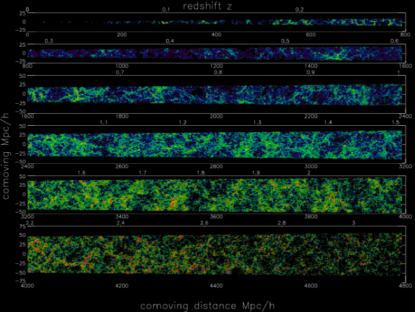
Figure 1: Light cone for a $1.4^{\circ}\times 1.4^{\circ}$ field out to $z=3.2$. All galaxies above an apparent magnitude limit $K_{s}(AB)<24$ are shown, where intensity corresponds to the logarithmic density and the color denotes the offset from the evolving red sequence.

3 Results

In this section we first compare our model to directly measured properties of real samples such as their distribution in apparent magnitude and redshift. We then consider derived properties which require an increasing number of additional assumptions, moving from the evolution of rest-frame luminosity functions to that of stellar mass distributions. Finally we illustrate the large changes predicted for the distribution of galaxies in rest-frame colour and absolute magnitude over the redshift range $0<z<3$. This gives a good impression of the interplay between the various mechanisms that determine the luminosity and colour of galaxies in our model.

All magnitudes are in the $AB$ system (rather than Vega) unless stated otherwise.

3.1 Number Counts

In Fig. 2 we compare predicted galaxy counts obtained from a mock survey of a $2\,\sq^{\circ}$ area to observational counts from a number of different surveys. In the $BRI$ bands we use counts over a $0.2\,\sq^{\circ}$ area in the HDF-N direction by Capak et al. (2004). In the $K_{s}$ band we use both the “wide” area ($320$ arcmin² distributed over various fields) counts of Kong et al. (2006) and the deeper, but smaller area counts in the CDF and HDF-S directions (6 and 7.5 arcmin² respectively) by Saracco et al. (2001). It is worth noting that for the $BRI$ bands we were able to use the filter transmission curves appropriate for the Subaru survey, whereas for the $K$ band different effective transmission curves apply for the different surveys and we have not taken this into account. In order to quantify the effect of “cosmic variance” (the fact that large statistical fluctuations are expected in surveys of this size not only from counting statistics but also from large-scale structure along the line-of-sight) we split up our $2\,\sq^{\circ}$ mock survey into 72 fields of size $100$ arcmin². The $1\sigma$ scatter among counts in these different areas is shown as a grey shaded area surrounding the predicted means for $BRI$ and for the brighter $K$ magnitudes. For the fainter $K$ magnitudes we split our mock survey into smaller subfields, each with an area of $\sim 11$ arcmin². The $1\sigma$ variations among these subfields are shown by the hatched band surrounding the predicted $K$ counts at fainter magnitudes. Note that this procedure may still somewhat underestimate the cosmic variance since the different subfields are not truly independent, but all lie within a single $1.4^{\rm o}\times 1.4^{\rm o}$ mock survey.

In the light of this limitation, and keeping in mind that our dust-model is still rather simple, it is quite surprising to see the excellent agreement of the data with our predictions in all three optical bands. Agreement at $K$ is less good, and there appears to be a significant disrepancy faintward of $K_{AB}\sim 21$. The model predicts almost twice as many galaxies as are observed at $K_{AB}\sim 23$, although the agreement is again acceptable at $K_{AB}\sim 24.5$. This disagreement appears well outside the statistical errors, but it should be borne in mind that $K$ magnitudes are extremely difficult to measure at such faint levels, and it is possible that the measured quantity does not correspond to the total magnitude assumed in our modelling.

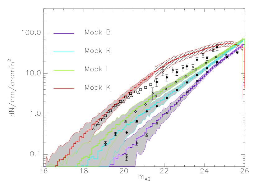
Figure 2: Predicted galaxy counts per unit area in four bands compared to a survey in the HDF-N direction ($0.2\,\sq^{\circ}$) in $BRI$ and to a number of “wide field” surveys at $K_{s}$ (total of $320$ arcmin²), as well as to deep observations at $K_{s}$ in the CDF and HDF-S directions (6 and 7.5 arcmin² respectively). The grey shaded error bands show $1\sigma$ field-to-field variations assuming an area of $100$ arcmin², whereas the hatched error bands show the expected variations for a smaller square field of area $\sim 11$ arcmin².

3.2 Redshift Distributions for $K$-selected samples

In Fig. 3 we give the redshift distributions predicted for apparent magnitude limited galaxy samples complete for $K\leq 21.8$, $K\leq 23.3$, and $K\leq 25.8$. We compare the first of these to data for a 52 arcmin² field from K20 (Cimatti et al., 2002b) and for a 160 arcmin² overlapping field from GOODS (Mobasher et al., 2004). (Note that the name K20 comes from the survey limit in the Vega system. The two systems are approximately related by $K_{AB}=K_{\rm Vega}+1.83$.). At the intermediate depth we compare to the photometric redshift distribution obtained by Caputi et al. (2006) for a 131 arcmin² field in the direction of the Chandra Deep Field South (CDF-S). For the faintest magnitude limit we compare to the photo-$z$ distribution of a much smaller 4 arcmin² area in the Subaru Deep Field, as obtained by Kashikawa et al. (2003). Again we split up our simulated field into sub-fields of size $100$ arcmin² ($4$ arcmin² for $K\leq 24$) in order to get an estimate of the expected $1\sigma$ scatter, which we indicate by grey shaded areas. For these small fields cosmic variance is quite substantial and the counts can be influenced significantly by individual galaxy clusters. This effect is clearly visible in the K20 and GOODS data, where a pronounced spike is present at $z\simeq 0.7$. In addition, systematic problems with the photometric redshift determinations might distort the redshift distributions in some ranges.

Despite these uncertainties, our model predictions appear somewhat high over the redshift range $0.5<z<1.5$ for the K20 and GOODS samples. The deeper $K\leq 23.3$ observations are overpredicted by a factor of 2 to 3 over the range $1<z<3$. For the faintest sample there is an apparent overprediction by a somewhat smaller factor over this same redshift range. Comparing with Fig. 2, we see that the total overprediction at each of these magnitudes is consistent with that seen in the counts themselves, although it should be borne in mind that the CDF-S field is common to both datasets. The differences we find are larger than the predicted cosmic variance so they presumably indicate problems with the model (incorrect physics?) with the observational data (systematics in the magnitudes or photo-$z$’s) or both.

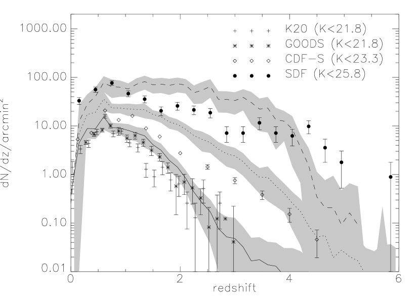
Figure 3: Predicted redshift distributions for galaxies to a magnitude limit of $K\leq 21.8$ (solid), 23.3 (dotted), and 25.8 (dashed). These are compared to observational results from K20 and GOODS ($K\leq 21.8$), from CDF-S ($K\leq 23.3$) and from SDF ($K\leq 25.8$). The latter two are derived purely from photometric redshift estimates. Error bars on the observational points are based on counting statistics only. Grey shaded areas indicate the $1\sigma$ field-to-field scatter assuming an area of $100$ arcmin² for the two brighter magnitude limits and $4$ arcmin² for $K\leq 25.8$.

3.3 Luminosity Function evolution

Croton et al. (2006) demonstrated that at $z=0$ the luminosity function (LF) for our model agrees well with observation both in $b_{J}$ and in $K$. Splitting galaxies according to their intrinsic colours, these authors also found quite good fits to the LF’s for red and blue galaxies separately, with some discrepancies for faint red galaxies. Here we compare the evolution of the LF predicted by our model in rest-frame $B$ and $K$ band with recent observational results.

3.3.1 The B-band Luminosity Function

In Fig. 4 we compare the evolution of the rest frame $B$-band LF predicted by our simulation to results from the DEEP2 survey (Willmer et al., 2005). As a $z=0$ standard we use the local LF from the 2dF survey Norberg et al. (2002). This is compared with our model in the top-left panel and is repeated as a thin red line in each of the other panels, where the high redshift data are indicated by points with error bars. Our predicted LF is shown in each panel as a solid line with a grey area indicating the $1\sigma$ scatter to be expected for an estimate from a survey similar in effective volume to the observational survey. (Note that in all cases the Millennium Simulation is much larger than this effective volume, so that counting noise uncertainties in the prediction are negligible.)

At $z=0$ the agreement between model and observation is excellent. This is a consequence of the fact that Croton et al. (2006) and De Lucia et al. (2006) adjusted model parameters in order to optimise this agreement. However, over the full redshift range from $z=0.2$ to $1.2$ the predicted LF’s agree with the DEEP2 data at the $1\sigma$ level or better. On closer examination, it appears that the model somewhat overpredicts the observational abundance fainter than the knee of the luminosity function, by a factor $\sim 1.5$ depending on redshift. On the other hand, at the higher redshifts very luminous galaxies appear slightly more abundant in the real data than in the model. It is important to keep in mind that our dust model has a strong influence here, and plausible modifications to it might account for either or both of these minor discrepancies. In general, the agreement with the data seems quite impressive, at least in this band and over this redshift range.

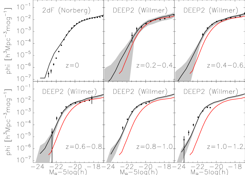
Figure 4: Comparison of the rest-frame $B$-band LF predicted by our simulation for redshifts in the range $0<z<1.2$ to observational estimates from Norberg et al. (2002) at $z=0$ and from Willmer et al. (2005) at higher redshifts. The local LF of the upper left panel is repeated as a thin red line in each of the other panels. A grey shaded region surrounding each model prediction shows the $1\sigma$ scatter expected in observational estimates based on samples similar in size to the corresponding observational sample.

3.3.2 The K-band Luminosity Function

Model predictions for the rest-frame $K$-band LF should, in principle, be more robust than predictions for the rest-frame $B$-band, because the effects of our uncertain dust modelling are then much weaker. On the other hand, observational determinations of the LF at rest-frame $K$ are more uncertain than at rest-frame $B$, because the magnitudes of high redshift galaxies must then be inferred by extrapolation beyond the wavelength region directly measured, rather than interpolated between the observed bands. This situation is improving rapidly as deep data at wavelengths beyond 2$\mu$ become available from Spitzer.

As can be seen in Fig. 5, our predictions for the evolution of the rest-frame $K$-band LF show the same behaviour as for the $B$-band. The local result from Cole et al. (2001) is reproduced well, as illustrated in the upper left panel and already demonstrated in Croton et al. (2006). The observed $z=0$ function is reproduced as a thin red line in the other panels in order to make the amount of evolution more apparent. At higher redshifts we compare with observational determinations from Pozzetti et al. (2003) for the 52 arcmin² of the K20 survey, from Feulner et al. (2003) for the 600 armin² of the MUNICS sample and from Saracco et al. (2006) for a 5.5 arcmin² area in the HDF-S. In these plots we give error bars as quoted by the original papers, but we note that these are based on counting statistics only and additional uncertainties are expected due to clustering, particularly for the smaller fields. Furthermore, photo-$z$’s are used for a significant number of galaxies in these determinations which may lead to additional systematic uncertainties in the results. Given the scatter between the various observational determinations, the disagreements between model and data do not look particularly serious. The models do appear to overpredict the abundance of galaxies near the knee of the luminosity function, perhaps by a factor of 2 at the highest redshift, echoing the discrepancies found above when comparing with $K$-band galaxy counts and redshift distributions.

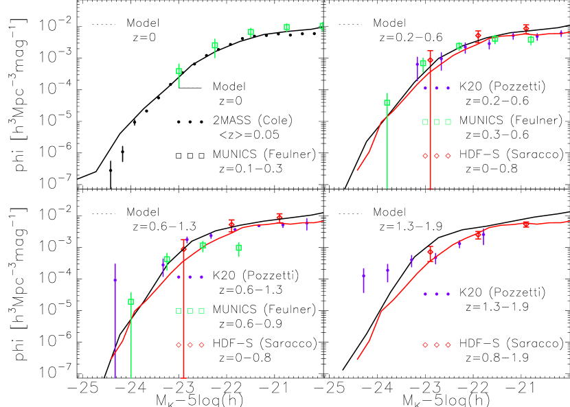
Figure 5: Comparison of the evolution predicted for the rest-frame $K$-band LF to observational determinations from Cole et al. (2001) at low $z$ (upper left panel, repeated as a thin red line in the other panels) and from Pozzetti et al. (2003), Feulner et al. (2003) and Saracco et al. (2006) at higher redshifts.

3.3.3 Evolution of Luminosity Function parameters

In order to display the evolution of the luminosity function in our models more effectively, we have fit Schechter (1976) functions to the simulation data for the rest-frame $B$ and $K$-bands at every stored output time. In most cases these functions are a good enough fit to give a fair representation of the numerical results. In Fig. 6 we plot the evolution with redshift of the parameters $\Phi^{*}$ and $M^{*}$ and of the volume luminosity density, $j=\Phi^{*}L^{*}\Gamma(\alpha+2)$ using thick solid lines, and we compare with fits to observational data. For each observational point in the $K$-band panels we indicate the (often broad) redshift range to which it refers by a horizontal bar. The vertical bar indicates the uncertainty quoted by the original authors.

Not surprisingly, the results of the last section are confirmed. For the model $\Phi^{*}$ increases slightly with redshift out to about $z=1.5$, whereas the observations imply a relatively steep decline over this same redshift range. This holds for both photometric bands. For $M^{*}$ we see brightening both in the models and in the observations, but the effect is more pronounced in the latter. In $K$ the models predict $M^{*}$ to be almost independent of redshift. Derivations of $\Phi^{*}$ and $M^{*}$ from observational data using maximum likelihood techniques usually give results where the errors in the two quantities correlate in a direction almost parallel to lines of constant luminosity density. For this reason we expect $j$ to be more robustly determined from the data than either $\Phi^{*}$ or $M^{*}$ individually. It is interesting that the apparent deviations between data and model for $\Phi^{*}$ and $M^{*}$ largely compensate, so that the model predicts an evolution of $j$ which is quite similar to that inferred from the observations. This is particularly striking at rest-frame $B$. At rest-frame $K$ the observational error bars are still too large to draw firm conclusions, but a non-evolving luminosity density represents the data somewhat better than does our model, again confirming the conclusions we drew in earlier sections.

Figure 6: The evolution of the $\Phi^{*}$ and $M^{*}$ parameters of Schechter (1976) fits to luminosity functions in rest-frame $B$ and $K$ (with $\alpha$ held constant at the values indicated). We also show the evolution of the total luminosity density $j$ inferred from these parameters. In each panel the solid line denotes the model prediction and the symbols are data from different sources (with potentially different $\alpha$). The $B$ band data comprises observations from Poli et al. (2003, + symbols) and Faber et al. (2005, diamonds), who also provide a compilation from the literature (filled circles), whereas the $K$ band data are observations (diamonds) and a literature compilation (filled circles) from Saracco et al. (2006).

3.4 The evolution of the stellar mass function

The evolution of the abundance of galaxies as a function of their stellar mass is one of the most direct predictions of galaxy formation models. It depends on the treatment of gas cooling, star-formation and feedback, but not directly on the luminous properties of the stars or on the dust modelling. (There remains an indirect dependence on the latter since observations of galaxy luminosities are typically used to set uncertain efficiency parameters in the modelling.) The stellar masses of galaxies can also be inferred relatively robustly from observational data provided sufficient observational information is available (e.g. Bell & de Jong 2001, Kauffmann et al 2003). At high redshift, however, such inferences become very uncertain unless data at wavelengths beyond 2$\mu$ are available (e.g. from Spitzer). The observationally inferred masses also depend systematically on the assumed Initial Mass Function for star formation (usually taken to be universal) and it is important to ensure that consistent assumptions about the IMF are made when comparing observation and theory.

Bearing in mind these caveats, Fig. 7 compares the mass functions predicted by our model to local data from Cole et al. (2001) as well as to high-redshift estimates from Drory et al. (2005), based on the MUNICS survey, and from Fontana et al. (2006) based on the MUSIC-GOODS data. The latter study uses data in the 3.6 to 8$\mu$ bands from Spitzer to constrain the spectral energy distributions of the galaxies and so should give substantially more reliable results at high redshift than the former. In Fig. 7 the model mass functions at $z>0$ are shown both before and after convolution with a gaussian in $\log M_{*}$ with standard deviation 0.25. This is intended to represent the uncertainty in the observational determinations of stellar mass. This error may be appropriate for the MUSIC-GOODS sample at all redshifts, but it is certainly too small to represent uncertainties in the MUNICS mass estimates at high redshift. We note that such errors weaken the apparent strength of the quasi-exponential cut-off at high masses. We neglect their effects at $z=0$.

Our model is nicely consistent with the observed mass function in the local Universe, but it clearly overpredicts the abundance of galaxies at redshifts between 1 and 3. The observed evolution relative to the $z=0$ function (indicated by the dashed line in each of the higher redshift panels) is strong, while the model prediction is rather more modest. In the stellar mass range $10^{10}$ to $10^{11}M_{\odot}$ where the observational estimats appear most reliable the overprediction reaches a factor of about 2 at $z=2$. This is nicely consistent with the conclusions we reached in earlier sections based on number counts, redshift distributions and luminosity functions, but unfortunately the scatter between the various observational determinations is large enough to prevent any firm conclusion.

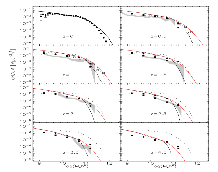
Figure 7: Evolution of the stellar mass function in the redshift range $z=0-4.5$. Local data are from Cole et al. (2001) and are repeated as a black dashed line in the higher redshift panels. High redshift data are taken from Drory et al. (2005, symbols) and Fontana et al. (2006, grey shaded areas). Model predictions are shown both with (red) and without (black) convolution with a normal distribution of standard deviation 0.25 representing measurement errors in $\log M_{*}$. At $z=0$ we consider the mass determinations precise enough to neglect this effect.

3.5 The evolution of the colour-magnitude relation

Recent studies of the high redshift galaxy population have often stressed the presence of massive objects with colours similar to those expected for fully formed and passively evolving ellipticals (e.g. Renzini, 2006, and references therein). This is usually presented as a potential problem for “hierarchical” models of galaxy formation where star formation and merging continue to play a major role in the build up of galaxies even at recent times. In order to illustrate how these processes are reflected in the colours and magnitudes of galaxies in our simulation, we show in Fig. 8 the colour-magnitude diagram for 10000 galaxies randomly sampled from a $2.5\times 10^{5}h^{-3}$Mpc³ volume at redshifts $z=0,$ 1, 2 and 3. At $z=0$ the well-known bi-modal distribution of colours is very evident. A tight red-sequence of passively evolving objects is present with a slope reflecting a relation between mass and metallicity. There is also a “blue cloud” of star-forming systems. A success of the model emphasised by Croton et al. (2006) is the fact that the brightest galaxies all lie on the red sequence at $z=0$. This is a consequence of including a treatment of “radio feedback” from AGN.

To allow better appreciation of the evolution to high redshift, we also show logarithmically spaced contours of the colour-magnitude distribution of all galaxies in a $1.5\times 10^{7}h^{-3}$Mpc³ volume as black contours in the panels of Fig. 8. The bluing of the upper envelope with increasing redshift is very clear and is consistent with passive evolution of the red sequence. We illustrate this by fitting a population synthesis model to the ridge line of the $z=0$ red sequence, assuming a single burst of star formation at $z=6$ and a metallicity which varies with stellar mass. This model is shown as a red line not only at $z=0$ (where it was fit) but also at the earlier redshifts. Notice that although there are galaxies with red sequence colours at all redshifts, the sequence becomes less and less well-defined at earlier times, with a substantial number of objects appearing redder than the passively evolving systems. These are compact, gas- and metal-rich galaxies where our model predicts very substantial amounts of reddening. Recent surveys of distant Extremly Red Objects have found substantial numbers of such systems (Cimatti et al., 2002a, 2003; Le Fèvre et al., 2005; Kong et al., 2006), but it remains to be seen if our model can account quantitatively for their properties.

The colours of galaxies in the blue cloud also become bluer at high redshift. This is a consequence of an increase in the typical ratio of current to past average star formation rate in these galaxies. The difference between star-forming systems and “true” red-sequence galaxies becomes blurred at high redshift in our model because of the increasingly important effects of dust.

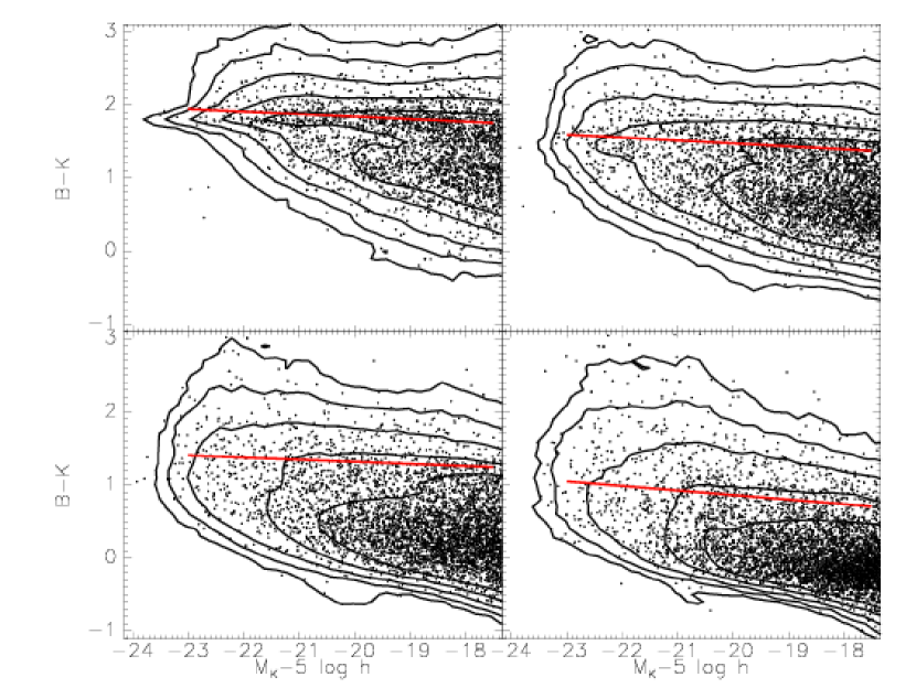
Figure 8: Evolution of the colour-magnitude distribution of galaxies in rest-frame $B$ and $K$ over the redshift range $z=[0,3]$. Randomly selected 10000 galaxies in a $2.5\times 10^{5}h^{-3}$Mpc³ volume of the simulation are plotted in each panel. For comparison purposes the distribution of a much larger sample in a $1.5\times 10^{7}h^{-3}$Mpc³ volume is indicated as logarithmically spaced contours. The red solid line indicates the colour magnitude relation predicted for stellar populations formed in a single burst at $z=6$ and evolving passively thereafter. The metallicity of the populations has been adjusted as a function of stellar mass to fit the ridge line of the $z=0$ red sequence.

4 Discussion and Conclusions

The model we have used in this paper is that of Springel et al. (2005) and Croton et al. (2006) and as updated by De Lucia & Blaizot (2006) and made public through the Millennium Simulation download site (see Lemson et al., 2006). Earlier work has compared this model to a wide range of properties of low redshift galaxies: their luminosity functions, their bi-modal luminosity-colour-morphology distribution and their Tully-Fisher relation (Croton et al., 2006); their spatial clustering as inferred from two-point correlations (Springel et al., 2005; Li et al., 2006; Meyer et al., 2006) and from fits to halo occupation distribution models (Wang et al., 2006; Weinmann et al., 2006); their HI gas content (Meyer et al., 2006); and their assembly histories within clusters (De Lucia et al., 2006; De Lucia & Blaizot, 2006). Although Croton et al. (2006) compared the evolution of the global star formation rate and the global black hole accretion rate of the model to observation, the current paper is the first to compare its predictions in detail with observations of high redshift galaxies.

Our comparison to galaxy counts, to redshift distributions and to observational estimates of luminosity and mass functions at high redshift paints a consistent picture despite large statistical uncertainties and some significant technical issues. Our model appears to have too many relatively massive galaxies at high redshift and these galaxies appear to be too red. Thus, while we fit optical galaxy counts well up to densities of 30 gal/mag/arcmin², we start to overpredict numbers in the $K$ band at densities above about 3 gal/mag/arcmin². This overabundance of apparently red galaxies shows up in the redshift distributions as an overprediction of the number of galaxies with $K\sim 23$ to 25 at redshift between about 1 and 3. These correspond to moderately massive systems near the knee of the luminosity function, and indeed, while our rest-frame $B$ luminosity functions appear compatible with observation out to $z\sim 1$, at rest-frame $K$ our luminosity functions are noticeably high beyond $z=0.5$ except possibly for the brightest objects. The problem shows up most clearly in our mass functions which overpredict observationally estimated abundances by about a factor of 2 at $z=2$. Apparently the mass function of galaxies evolved more strongly in the real Universe than in our simulation.

A galaxy formation model with similar basic ingredients to ours, but with important differences of detail has been independently implemented on the Millennium Simulation by Bower et al. (2006). This model is also publicly available at the download site. It fits low redshift galaxy luminosity functions as well as our model, but the comparisons which Bower et al. (2006) show to high-redshift luminosity and mass function data (essentially the same datasets we use here) demonstrate somewhat better agreement than we find in this paper. In the mass range $10^{10}<h^{2}M_{*}/M_{\odot}<10^{11}$ the abundances predicted by their model are lower than ours by about 20% at $z=1$ and by about 30% at both $z=2$ and $z=3.5$, despite the fact that at $z=0$ the two models agree very well. This is consistent with the fact that their model forms 20% of all its stars by $z=3.2$ and 50% by $z=1.65$ whereas the corresponding redshifts for our model are $z=3.6$ and $z=1.9$. These differences arise from details of the star formation and feedback models adopted in the two cases.

In summary, both the Bower et al. (2006) simulation and our own are consistent with most current faint galaxy data. Thus there seems no difficulty in reconciling the observed properties of distant objects with hierarchical galaxy formation. The fact that predictions from the two simulations differ at a level which can be marginally separated by the observations, means that currently accessible properties of distant galaxies can significantly constrain models of this type, and hence the detailed physics which controls the formation and the observable properties of galaxies. The fact that the model we test here apparently overpredicts the abundance of moderately massive galaxies at high redshift, despite the fact that late merging plays a major role in the build-up of its more massive galaxies (e.g. De Lucia et al., 2006; De Lucia & Blaizot, 2006), demonstrates that current data are still far from constraining the importance of this process. As the data improve, the models will have to improve also to remain consistent with them. This interplay between theory and observation should eventually lead to a more convincing and more complete picture of how galaxies came to take their present forms.

Acknowledgements: We thank Jeremy Blaizot, Darren Croton and Gabriella De Lucia for useful discussions of a number of technical issues which arose during this project. MGK acknowledges a PhD fellowship from the International Max Planck Research School in Astrophysics, and support from a Marie Curie Host Fellowship for Early Stage Research Training.

References

- Adelberger & Steidel (2000) Adelberger, K. L. & Steidel, C. C. 2000, ApJ, 544, 218
- Barnes & Hut (1986) Barnes, J. & Hut, P. 1986, Nature, 324, 446
- Blaizot et al. (2005) Blaizot, J., Wadadekar, Y., Guiderdoni, B., et al. 2005, MNRAS, 360, 159
- Bower et al. (2006) Bower, R. G., Benson, A. J., Malbon, R., et al. 2006, MNRAS, 370, 645
- Capak et al. (2004) Capak, P., Cowie, L. L., Hu, E. M., et al. 2004, AJ, 127, 180
- Caputi et al. (2006) Caputi, K. I., McLure, R. J., Dunlop, J. S., Cirasuolo, M., & Schael, A. M. 2006, MNRAS, 366, 609
- Cardelli et al. (1989) Cardelli, J. A., Clayton, G. C., & Mathis, J. S. 1989, ApJ, 345, 245
- Chen et al. (2003) Chen, H., Marzke, R. O., McCarthy, P. J., et al. 2003, ApJ, 586, 745
- Cimatti et al. (2003) Cimatti, A., Daddi, E., Cassata, P., et al. 2003, AAp, 412, L1
- Cimatti et al. (2002a) Cimatti, A., Daddi, E., Mignoli, M., et al. 2002a, AAp, 381, L68
- Cimatti et al. (2002b) Cimatti, A., Pozzetti, L., Mignoli, M., et al. 2002b, AAp, 391, L1
- Cole et al. (2001) Cole, S., Norberg, P., Baugh, C. M., et al. 2001, MNRAS, 326, 255
- Colless et al. (2001) Colless, M., Dalton, G., Maddox, S., et al. 2001, MNRAS, 328, 1039
- Croton et al. (2006) Croton, D. J., Springel, V., White, S. D. M., et al. 2006, MNRAS, 365, 11
- De Lucia & Blaizot (2006) De Lucia, G. & Blaizot, J. 2006, ArXiv Astrophysics e-prints: astro-ph/0606519
- De Lucia et al. (2004) De Lucia, G., Kauffmann, G., & White, S. D. M. 2004, MNRAS, 349, 1101
- De Lucia et al. (2006) De Lucia, G., Springel, V., White, S. D. M., Croton, D., & Kauffmann, G. 2006, MNRAS, 366, 499
- Devriendt & Guiderdoni (2000) Devriendt, J. E. G. & Guiderdoni, B. 2000, AAp, 363, 851
- Devriendt et al. (1999) Devriendt, J. E. G., Guiderdoni, B., & Sadat, R. 1999, AAp, 350, 381
- Drory et al. (2005) Drory, N., Salvato, M., Gabasch, A., et al. 2005, ApJL, 619, L131
- Faber et al. (2005) Faber, S. M., Willmer, C. N. A., Wolf, C., et al. 2005, ArXiv Astrophysics: astro-ph/0506044
- Feulner et al. (2003) Feulner, G., Bender, R., Drory, N., et al. 2003, MNRAS, 342, 605
- Fontana et al. (1999) Fontana, A., Menci, N., D’Odorico, S., et al. 1999, MNRAS, 310, L27
- Fontana et al. (2006) Fontana, A., Salimbeni, S., Grazian, A., et al. 2006, ArXiv Astrophysics: astro-ph/0609068
- Hockney & Eastwood (1981) Hockney, R. W. & Eastwood, J. W. 1981, Computer Simulation Using Particles (Computer Simulation Using Particles, New York: McGraw-Hill, 1981)
- Im et al. (2002) Im, M., Simard, L., Faber, S. M., et al. 2002, ApJ, 571, 136
- Inoue (2003) Inoue, A. K. 2003, PASJ, 55, 901
- Kashikawa et al. (2003) Kashikawa, N., Takata, T., Ohyama, Y., et al. 2003, AJ, 125, 53
- Kauffmann & Charlot (1998) Kauffmann, G. & Charlot, S. 1998, MNRAS, 294, 705
- Kauffmann et al. (1999) Kauffmann, G., Colberg, J. M., Diaferio, A., & White, S. D. M. 1999, MNRAS, 303, 188
- Kauffmann & Haehnelt (2000) Kauffmann, G. & Haehnelt, M. 2000, MNRAS, 311, 576
- Kauffmann et al. (1993) Kauffmann, G., White, S. D. M., & Guiderdoni, B. 1993, MNRAS, 264, 201
- Kitzbichler & White (2006) Kitzbichler, M. G. & White, S. D. M. 2006, MNRAS, 366, 858
- Kong et al. (2006) Kong, X., Daddi, E., Arimoto, N., et al. 2006, ApJ, 638, 72
- Kravtsov et al. (2004) Kravtsov, A. V., Gnedin, O. Y., & Klypin, A. A. 2004, ApJ, 609, 482
- Le Fèvre et al. (2005) Le Fèvre, O., Paltani, S., Arnouts, S., et al. 2005, Nature, 437, 519
- Lemson et al. (2006) Lemson, G. et al. 2006, ArXiv Astrophysics: astro-ph/0608019
- Li et al. (2006) Li, C., Kauffmann, G., Jing, Y. P., et al. 2006, MNRAS, 368, 21
- Meyer et al. (2006) Meyer, M. J., Zwaan, M. A., Webster, R. L., Brown, M. J. I., & Staveley-Smith, L. 2006, ArXiv Astrophysics e-prints: astro-ph/0608633
- Mobasher et al. (2004) Mobasher, B., Idzi, R., Benítez, N., et al. 2004, ApJL, 600, L167
- Norberg et al. (2002) Norberg, P., Cole, S., Baugh, C. M., et al. 2002, MNRAS, 336, 907
- Poli et al. (2003) Poli, F., Giallongo, E., Fontana, A., et al. 2003, ApJL, 593, L1
- Pozzetti et al. (2003) Pozzetti, L., Cimatti, A., Zamorani, G., et al. 2003, AAp, 402, 837
- Reddy et al. (2006) Reddy, N. A., Steidel, C. C., Fadda, D., et al. 2006, ApJ, 644, 792
- Renzini (2006) Renzini, A. 2006, ARAA, 44, 141
- Saracco et al. (2006) Saracco, P., Fiano, A., Chincarini, G., et al. 2006, MNRAS, 367, 349
- Saracco et al. (2001) Saracco, P., Giallongo, E., Cristiani, S., et al. 2001, AAp, 375, 1
- Seljak et al. (2005) Seljak, U., Makarov, A., McDonald, P., et al. 2005, Physical Review, 71, 103515
- Somerville et al. (2004) Somerville, R. S., Moustakas, L. A., Mobasher, B., et al. 2004, ApJL, 600, L135
- Spergel et al. (2003) Spergel, D. N., Verde, L., Peiris, H. V., et al. 2003, ApJS, 148, 175
- Springel (2005) Springel, V. 2005, MNRAS, 364, 1105
- Springel et al. (2006) Springel, V., Frenk, C. S., & White, S. D. M. 2006, Nature, 440, 1137
- Springel et al. (2005) Springel, V., White, S. D. M., Jenkins, A., et al. 2005, Nature, 435, 629
- Springel et al. (2001a) Springel, V., White, S. D. M., Tormen, G., & Kauffmann, G. 2001a, MNRAS, 328, 726
- Springel et al. (2001b) Springel, V., Yoshida, N., & White, S. D. M. 2001b, New Astronomy, 6, 79
- Wang et al. (2006) Wang, L., Li, C., Kauffmann, G., & de Lucia, G. 2006, MNRAS, 371, 537
- Weinmann et al. (2006) Weinmann, S. M., van den Bosch, F. C., Yang, X., et al. 2006, ArXiv Astrophysics e-prints: astro-ph/0606458
- White & Frenk (1991) White, S. D. M. & Frenk, C. S. 1991, ApJ, 379, 52
- Willmer et al. (2005) Willmer, C. N. A., Faber, S. M., Koo, D. C., et al. 2005, ArXiv Astrophysics: astro-ph/0506041