Statefinder Revisited

Abstract

The quality of supernova data will dramatically increase in the next few years by new experiments that will add high-redshift supernova to the currently known ones. In order to use this new data to discriminate between different dark energy models, the statefinder diagnostic was suggested S and investigated by Alam et al.A in the light of the proposed SuperNova Acceleration Probe (SNAP) satellite. By making use of the same procedure presented by these authors, we compare their analyzes with ours, which shows a more realistic supernovae redshift distribution and do not assume that the intercept is known. We also analyzed the behavior of the statefinder pair {r,s} and the alternative pair {s,q} in the presence of offset errors.

Introduction

Recent observations from type Ia supernovae measurements, cosmic microwave background radiation and gravitational clustering suggest the expansion of the universe is accelerated.

In order to explain this cosmic acceleration a form of negative-pressure matter called dark energy was suggested. The simplest and most popular candidate is Einstein’s cosmological constant. Many others candidates for dark energy have been proposed, including scalar fields with a time dependent equation of state, quartessence, modified gravity, branes, etc. Confrontation between these models and currently observational data doesn’t say much Q , mainly because most of them have $\Lambda$CDM as a limiting case in the redshift range already observed. The SNAP (SuperNovae Acceleration Probe) satellite is expected to observe $\sim 2000$ supernovae per year with redshift up to $z=1.7$. To differentiate models using the new available data, Sahni et al. S introduced the statefinder diagnostic, that is based on the dimensionless parameters {r,s}, which are constructed with the scale factor and its time derivatives.

In this work we applied the statefinder to a SNAP-like supernovae distribution and analyzed its behavior in the presence of systematic and random systematic, beyond statistical errors.

I Dark Energy Models

Assuming a Friedman-Robertson-Walker (FRW) metric, the Einstein’s equations reduce to:

$$H^{2} = \frac{8\pi G}{3}\sum_{i}\rho_{i}-\frac{kc^{2}}{a^{2}}$$ (1)

$$\frac{\ddot{a}}{a} = -\frac{4\pi G}{3}\sum_{i}(\rho_{i}+3\frac{p_{i}}{c^{2}})$$ (2)

where a is the scale factor of the FRW metric, H is the Hubble parameter, and the sum is over all the components present in the scenario in study.

In the following we assume that the matter content of the universe is given by dark matter ($p_{m}=0$) and dark energy with an equation of state in the form $p_{x}=p_{x}(\rho_{x})$. We also take $c=1$ and consider a flat universe ($k=0$).

Table 1: Redshift distribution. The value of z represent the upper edge of each bin K

z	0.1	0.2	0.3	0.4	0.5	0.6	0.7	0.8	0.9	1.0	1.1	1.2	1.3	1.4	1.5	1.6	1.7
N(z)	0	35	64	95	124	150	171	183	179	170	155	142	130	119	107	94	80

The focus of our discussion will be in the four models listed below:

1. Cosmological Constant ($w_{x}=p_{x}/\rho_{x}=-1$)
   The cosmological constant model represents a constant energy density. In this model, the Hubble parameter has the form:

   $$H(z)=H_{0}[\ \Omega_{m0}(1+z)^{3}+1-\Omega_{m0}]^{\frac{1}{2}}$$ (3)

2. Quiessence ( $-1/3>w_{x}=p_{x}/\rho_{x}=cte>-1$)
   This is the next simplest example of dark energy model, and gives rise to a Hubble parameter like:

   $$H(z)=H_{0}[\ \Omega_{m0}(1+z)^{3}+\Omega_{X0}(1+z)^{3(1+w)}]^{\frac{1}{2}}$$ (4)

3. Quintessence ( w = w ( t ) )
   Representing a self-interacting scalar field minimally coupled to gravity. In this model, we have:

   $$\rho_{\phi} = \frac{1}{2}\dot{\phi}(z)^{2}+V(\phi(z))$$ (5)

   $$p_{\phi} = \frac{1}{2}\dot{\phi}(z)^{2}-V(\phi(z))$$ (6)

   We shall focus on a special kind of quintessence model that has a tracker like solution, with the following potential: $V(\phi)=\phi(z)^{-\alpha}(\alpha>0)$. In this case, it can be shown that the present energy density of the dark energy is almost independent of initial conditions.

4. Chaplygin Gas
   A different kind of solution is provided by the Chaplygin gas model. In this model, the Hubble parameter takes the form:

   $$H(z)=H_{0}\bigg{[}\Omega_{m0}(1+z)^{3}+\frac{\Omega_{mo}}{\kappa}\sqrt{\frac{A}{B}(1+z)^{6}}\bigg{]}^{\frac{1}{2}}$$ (7)

   where

   $$\kappa=\frac{\rho_{mo}}{\rho_{ch0}}$$ (8)

   The Chaplygin gas behaves like a cosmological constant for small z (late times) and like pressureless dust for large z (early times).

It is important to note that for all models presented previously, the luminosity distance is :

$$\frac{D_{L}(z)}{1+z}=\int_{0}^{z}\frac{dz^{\prime}}{H(z^{\prime})}$$ (9)

with $H(z)$ given by the model dependent expressions presented before.

II The Statefinder

The properties of dark energy, as we have seen, are very model dependent. In order to differentiate between the presented models, Sanhi et al.S , proposed the statefinder diagnostic. The parameters, {r,s}, are a complement to the already known deceleration parameter, and help the discrimination when the later contains degeneracies. By definition:

$$q=-\frac{\ddot{a}}{aH^{2}}\equiv\frac{1}{2}(1+3w\Omega_{X})$$ (10)

$$r\equiv\frac{\ddot{a}}{aH^{3}}=1+\frac{9w}{2}\Omega_{X}(1+w)-\frac{3}{2}\Omega_{X}\frac{\dot{w}}{H}$$ (11)

$$s\equiv\frac{r-1}{3(q-\frac{1}{2})}=1+w-\frac{1}{3}\frac{\dot{w}}{wH}$$ (12)

III Dark Energy from SNAP data

Type Ia supernovae are considered standard candles, used to map the expansion history, and its observations lead to the behavior of the scale factor with time. In order to study the data in a model independent way, we use a parametrization for the dark energy density, presented by Sahni et al. S . We express the energy density as a power series up to second order in z: $\rho_{DE}=\rho_{c0}(A_{1}+A_{2}x+A_{3}x^{2})$, where $x=1+z$. For this Ansatz, the Hubble parameter takes the form:

$$H(x)=H_{0}(\Omega_{m0}x^{3}+A_{1}+A_{2}x+A_{3}x^{2})^{\frac{1}{2}}$$ (13)

equation (13) together with equation (9) provides an expression for the luminosity distance, which we shall investigate, using the statefinder parameters, in the light of a SNAP-like experiment simulation.

To simulate the data, we use a binned approach for a SNAP distribution shown in the Table I. We also include $300$ supernovae in the first bin. These low redshift supernovae are expected from the SNFactory (Nearby Supernovae Factory) experiment and are important in reducing the systematic errors. The SNFactory proposal is to provide data to calibrate high redshift experiments, like the SNAP, and then reduce the errors involved.

The luminosity distance of equation (9) is measured in terms of the apparent magnitude, which can be written as:

$$m(z) = 5\log{d(z)}+$$ (14)

$$[M+25-5\log{(H_{0}/(100km/s/Mpc)})]$$

where M is the absolute magnitude of the supernova and the expression in brackets is called intercept.

Following what was done by Kim et al. K , we consider a random irreducible systematic error of $0.04*(z_{med}/1.7)$ (here $z_{med}$ is the redshift in the middle of each bin), added in quadrature to a constant statistical error of $0.15mag$ and study the behavior of the statefinder parameter with this synthetic data. We performed a Monte Carlo simulation considering the intercept exactly known and totally unknown. As a second step, we study the situation where offset errors are present, and its consequences in the statefinder.

IV Results

In the figures 1 to 9 we present the results from simulated data. According to SNAP’s specifications, we generated $500$ data sets having $\Lambda$CDM as a fiducial model. For each of this experiments we calculated the best fitting parameters $A_{1}$ and $A_{2}$ for equation (13) and reconstructed the statefinders $r(z)$ e $s(z)$. The figures below show the mean value of the parameters, which were calculated as:

$$<(r)> = \frac{1}{500}\sum_{i=1}^{500}r_{i}(z)$$ (15)

$$<(s)> = \frac{1}{500}\sum_{i=1}^{500}s_{i}(z)$$ (16)

$$<(q)> = \frac{1}{500}\sum_{i=1}^{500}q_{i}(z)$$ (17)

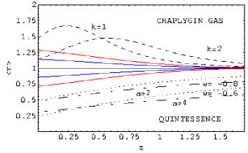
Figure 1: Shows $<r>$ as a function of redshift. The blue contour represent $1\sigma$ and the red contour $2\sigma$ confidence levels, in the presence of statistical errors with a known intercept.The line $<r>=1$ represents the $\Lambda$CDM fiducial model. The dashed lines above the $\Lambda$CDM are Chaplygin gas with parameters $k=1$ and $k=2$. The dotted lines below it are quiessence models with $w=-0.6$ and $w=-0.8$, and the dotted-dashed lines are quintessence models with $\alpha=2$ and $\alpha=4$.

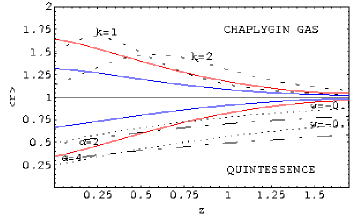
Figure 2: Analog to figure 1, but here in the presence of random systematic and statistical errors, with an unknown intercept.

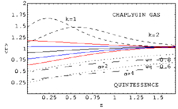
Figure 3: Shows $<r>$ as a function of redshift. Again, the blue and red contours are $1\sigma$ and $2\sigma$ confidence levels, in these we considered a known intercept in the presence of statistical error and a systematic error of $+0.03mag$.The dotted, dot-dashed and dashed lines are the same as in figure 1.

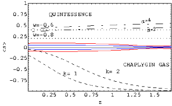
Figure 4: Shows $<s>$ as a function of redshift in the presence of statistical error. The colored contours, dotted, dot-dashed and full lines represent the same models as in figure 1.

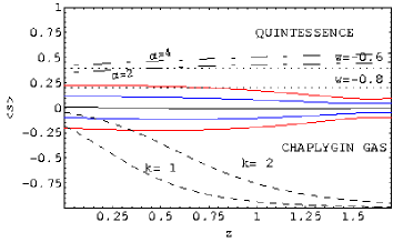
Figure 5: Analog to figure 4, but here in the presence of random systematic and statistical errors, with an unknown intercept.

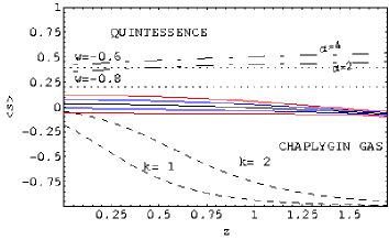
Figure 6: Shows $<s>$ as a function of redshift. Again, the blue and red contours are $1\sigma$and $2\sigma$ confidence levels, in this we considered a known intercept in the presence of statistical error and a systematical errors of $+0.03mag$.The dotted, dot-dashed and dashed lines are the same as in figure 1.

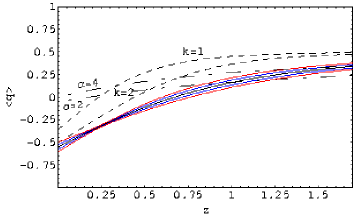
Figure 7: Shows $<q>$ as a function of redshift. The blue contour represent $1\sigma$ and the red contour $2\sigma$ confidence levels. The dashed lines are Chaplygin gas with parameters $k=1$ and $k=2$. The dotted-dashed lines are quintessence models with $\alpha=2$ and $\alpha=4$.

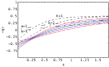
Figure 8: Analog to figure 7, but here in the presence of random systematic and statistical errors, with an unknown intercept.

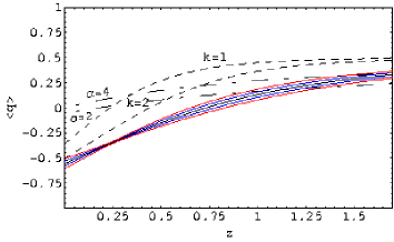
Figure 9: Shows $<q>$ as a function of redshift. Again, the blue and red contours are $1\sigma$ and $2\sigma$ confidence levels, in these we considered a known intercept in the presence of statistical error and a systematical error of $+0.03mag$.The dot-dashed and dashed lines are the same as in figure 7.

Next, we investigated the integrated averaged of the cosmological parameters, as suggested by Alam et al. A . For the cosmological constant model, the parameters are constant, but for many dark energy models the statefinder evolves (as it is clear in the figures presented previously), the integration of this quantities may then reduce the noise in the original data. The integration was done as follows:

$$\bar{r} = \frac{1}{z_{max}}\int_{0}^{z_{max}}r(z)dz$$ (18)

$$\bar{s} = \frac{1}{z_{max}}\int_{0}^{z_{max}}s(z)dz$$ (19)

$$\bar{q} = \frac{1}{z_{max}}\int_{0}^{z_{max}}q(z)dz$$ (20)

where $z_{max}=1.7$ . The expressions for r, s and q were calculated using equations 13, 11 and the first part of equation 12 for each experiment. The $500$ points obtained are plotted in figures 10 to 15:

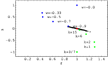
Figure 10: Shows the variation of $\bar{r}$ with $\bar{s}$ , in the presence of statistical error when the intercept is known. The red dot is the $\Lambda$CDM fiducial model. The blue dots above the $\Lambda$CDM are quiessence models with $w=0.0,-0.3,(-0.5),-0.7$ and $0.9$ respectively, from top to bottom. The green dots below $\Lambda$CDM are Chapligyn gas with $k=(3/7),1,2,6,15$, from bottom to top.

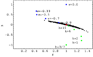
Figure 11: This is analogous to figure 10, although here we considered an intercept not known and included statistical and random systematic errors.

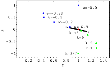
Figure 12: Show the variation of $\bar{r}$ with $\bar{s}$ when the intercept is known, in the presence of statistical error and systematic error of $+0.03mag$. The red, blue and green dots are the same as in figure 10.

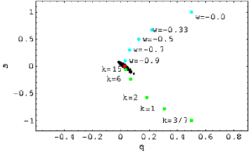
Figure 13: Shows the variation of $\bar{s}$ with $\bar{q}$, in the presence of statistical error when the intercept is known. The red dot is the $\Lambda$CDM fiducial model. The blue dots above the $\Lambda$CDM are quiessence models with $w=0.0,-0.3,(-0.5),-0.7$ and $0.9$ respectively, from top to bottom. The green dots below $\Lambda$CDM are Chapligyn gas with $k=(3/7),1,2,6,15$, from bottom to top.

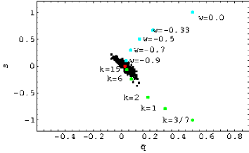
Figure 14: This is analogous to figure 13, although here we considered an intercept not known and included statistical and random systematic errors.

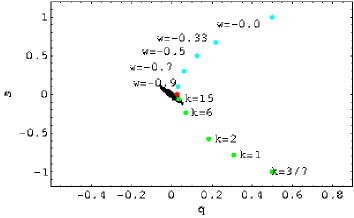
Figure 15: Show the variation of $\bar{s}$ with $\bar{q}$ when the intercept is known, in the presence of statistical and systematic error of $+0.03mag$. The red, blue and green dots are the same as in figure 13.

V Discussion

Our results suggest that the statefinder is a good diagnostic for dark energy models, although some care must be taken in applying it to data. As expected, the presence of random systematic error and an unknown intercept just added more possible models than those allowed by statistical errors only. There is little problem in this, once the fiducial model is at least within the $2\sigma$ contours (Figures 2, 5 and 8).

The presence of offset errors had different outcomes. For a positive offset, the parameters r and s suffered a small reduction in relation to the fiducial model, but in different redshift ranges (r for small and s for high redshift). A consequence of this arises when we compare the integrated averages of the pair {r,s}. In Figure 12 the points are shifted to the negative direction of both axes of the ellipse, resulting a data set where the fiducial model (red point) is on the edge of the distribution. The same kind of shift is observed for a negative offset, but in this case to the positive direction of the axes. So, in order to use the statefinder as a diagnostic, we must be able to control the offset error below $0.03mag$.

It is interesting to observe the behavior of the deceleration parameter when systematic errors were involved. It does present a very small reduction (positive offset) at high redshift, but it is irrelevant in front of that suffered by r or s. Comparing figures 10 and 13 we could say, as suggested by Alam et al. A , that the pair {q,s} is even a better diagnostic than {r,s}, once it restricts the area of the phase space filled by the data. However, if there is a systematic error present, the points will be shifted to the negative direction of the q axis only (figure 15), letting the distance between the data and the fiducial model bigger than those in figure 12.

Therefore, we concluded that the statefinder pair {r,s} is a better diagnostic than the pair {s,q}, when the involved systematic errors are not random.

Acknowlegments

The author is grateful to Ioav Waga for suggesting this problem and for extensive discussion and encouragement throughout the course of the work. This work was supported by the Brazilian research agency CNPq.

References

V. Sahni, T. D. Saini, A. A. Starobinsky, U. Alam, JETP Lett. 77, 201 (2003)

K. D. Evans , I. K. Wehus , O. Gron , O. Elgaroy, Astron.Astrophys.,430, 399 (2005)

U. Alam, V. Sahni , T. D. Saini and A. A. Starobinsky, Mon.Not.Roy.Astron.Soc., 344 1057,(2003)

A. G. Kim, E. V. Linder, R. Miquel and N. Mostek, Mon.Not.Roy.Astron.Soc. 347 909, (2004)

M. Goliath, R. Amanullah, P. Astier, A. Goobar and R. Pain, astro-ph/0104009