Scale dependence of halo and galaxy bias: effects in real space
Abstract
We examine the scale dependence of dark matter halo and galaxy clustering on very large scales (), due to non-linear effects from dynamics and halo bias. We pursue a two line offensive: high resolution numerical simulations are used to establish some old and some new results, and an analytic model is developed to understand their origins. Our simulations show: (i) that the dark matter power spectrum is suppressed relative to linear theory by on scales ; (ii) that, indeed, halo bias is non-linear over the scales we probe and that the scale dependence is a strong function of halo mass. High mass haloes show no suppression of power on scales , and only show amplification on smaller scales, whereas low mass haloes show strong, , suppression over the range . These results were primarily established through the use of the cross-power spectrum of dark matter and haloes, which circumvents the thorny issue of shot-noise correction. The halo-halo power spectrum, however, is highly sensitive to the shot-noise correction; we show that halo exclusion effects make this sub-Poissonian and a new correction is presented. Our results have special relevance for studies of the baryon acoustic oscillation features in the halo power spectra. Non-linear mode-mode coupling: (i) damps these features on progressively larger scales as halo mass increases; (ii) produces small shifts in the positions of the peaks and troughs which depend on halo mass. We show that these effects on halo clustering are important over the redshift range relevant to such studies , and so will need to be accounted for when extracting information from precision measurements of galaxy clustering.
Our analytic model is described in the language of the ‘halo-model’. The halo-halo clustering term is propagated into the non-linear regime using ‘1-loop’ perturbation theory and a non-linear halo bias model. Galaxies are then inserted into haloes through the Halo Occupation Distribution. We show that, with non-linear bias parameters derived from simulations, this model produces predictions that are qualitatively in agreement with our numerical results. We then use it to show that the power spectra of red and blue galaxies depend differently on scale, thus underscoring the fact that proper modeling of nonlinear bias parameters will be crucial to derive reliable cosmological constraints. In addition to showing that the bias on very large scales is not simply linear, the model also shows that the halo-halo and halo-dark matter spectra do not measure precisely the same thing. This complicates interpretation of clustering in terms of the stochasticity of bias. However, because the shot noise correction is non-trivial, evidence for this in the simulations is marginal.
pacs:
98.80.-kI Introduction
Statistical analysis of the large scale structures observed in galaxy surveys can provide a wealth of information about the cosmological parameters, the underlying mass distribution and the initial conditions of the Universe. The information is commonly extracted through measurement of the two-point correlation function Hawkins et al. (2003); Eisenstein et al. (2005) or its Fourier space analogue the Power spectrum Tegmark et al. (2004); Cole et al. (2005); Tegmark et al. (2006); Percival et al. (2006, 2006). When further combined with high precision measurements of the temperature anisotropy spectrum from the Cosmic Microwave Background very strong constraints can be imposed on the initial conditions, the energy content, shape and evolution of the Universe Spergel et al. (2006).
For homogeneous and isotropic Gaussian Random fields, such as is supposed for the post inflationary density field of Cold Dark Matter (hereafter CDM) fluctuations, each Fourier mode is independent, and thus all of the statistical properties of the field are governed by the power spectrum. However, non-linear evolution of matter couples the Fourier modes together, and power is transfered from large to small scales Peebles (1980); Bernardeau et al. (2002). Consequently, it is non-trivial to relate the observed structures to the physics of the initial conditions. Further, since one typically measures not the mass, but the galaxy fluctuations, some understanding of the mapping from one to the other is required. This mapping, commonly referred to as galaxy bias, encodes the salient physics of galaxy formation.
One last complication must be added: since galaxy positions are inferred from recession velocities using Hubble’s law, and because each galaxy possesses its own peculiar velocity relative to the expansion velocity, a non-trivial distortion is introduced to the clustering on all scales from the velocity field. These velocity effects are commonly referred to as redshift space distortions. Thus one must accurately account for non-linear evolution of matter fluctuations, bias and redshift space distortions in order to extract precise information from large scale structure surveys and this remains one of the grand challenges for modern physical cosmology.
In this paper, we investigate the issue of bias in some detail, through both numerical and analytic means. We focus on real space effects and reserve our results from redshift space for a subsequent paper. Our numerical work focuses on the generation of multiple realizations of the same cosmological model, in two different box sizes. This allows us to construct halo catalogues spanning a large dynamic range in mass that are largely free from discreteness fluctuations and the multiple realizations allow us to derive errors that are ‘true errors from the ensemble’. We use this data to show that not only is halo clustering on very large scales scale dependent, but that the scale dependence is a strong function of halo mass. These results are completely expected given the standard theoretical understanding of dark matter haloes based on the ‘peak-background split’ argument Cole & Kaiser (1989); Mo & White (1996); Mo, Jing & White (1997); Sheth & Tormen (1999); Scoccimarro et al. (2001).
Our analytic approach to modelling these trends can be summarized as follows.
-
•
Haloes are biased tracers of the mass distribution. To describe this bias, we assume that the bias relation between the halo density field and the dark matter field is non-linear, local and deterministic. This allows us to use the formalism of Fry & Gaztañaga (1993); Mo, Jing & White (1997). In order for the local model to hold, one must integrate out small scales where locality is almost certainly violated. This can be done in real space by smoothing small-scale fluctutations, or in Fourier space by considering small wavenumbers 111Several broad classes of bias model may be defined: local Coles (1993) and non-local Kaiser (1984); Dekel & Rees (1987); Catelan, Matarrese & Porciani (1998); Catelan, Porciani & Kamionkowski (2000); Matsubara (1999); linear or non-linear Cen & Ostriker (1992); Fry & Gaztañaga (1993); Heavens, Matarrese & Verde (1998); Mann, Peacock & Heavens (1998); Benson et al. (2000); Peacock & Smith (2000); Cen & Ostriker (2000); and deterministic or stochastic Scherrer & Weinberg (1998); Dekel & Lahav (1999). With the exception of stochastic, local, linear biasing, all these prescriptions result in some non-trivial degree of scale dependence. Note that when weakly nonlinear scales are discussed, as we do in this paper, it may not be entirely consistent to neglect nonlocality, which could potentially alter the predictions we present. Nonlocal bias can be looked for in observations by using higher-order statistics Frieman & Gaztañaga (1994); Feldman et al. (2001). However, we may take comfort in the fact that there is always a strong correlation between haloes and dark matter, since the former are built from the latter!.
-
•
The underlying CDM density field is then propagated into the non-linear regime using standard Eulerian perturbation theory techniques Bernardeau et al. (2002).
- •
Because we write the PT evolved halo density field as a series expansion we refer to this method as ‘Halo-PT’ theory.
Our results are particularly relevant for studies which intend to use the baryon acoustic oscillation feature (hereafter BAO) in the low redshift clustering of galaxies to derive constraints on the dark energy equation of state Eisenstein et al. (2005). The CDM transfer function that we have adopted throughout contains a significant amount of BAOs, and we give an accounting of the possible non-linear corrections from mass evolution and biasing that might influence the detection and interpretation of such features. Previous work in this direction has primarily focused on analysis of numerical simulations Meiksin, White & Peacock (1999); Seo & Eisenstein (2003, 2005); White (2005); Huff et al. (2006), although several analytic works have recently been presented: Crocce & Scoccimarro (2006b) derive the exact damping of BAOs in the Zel’dovich approximation and calculate it in the exact dynamics by re-summing perturbation theory; Jeong & Komatsu (2006) consider real space corrections to the power spectrum from one-loop PT; Guzik, Bernstein & Smith (2006) use the halo model, also in real space, to explore systematics; Eisenstein, Seo & White (2006); Eisenstein et al. (2006) consider a model of Lagrangian displacements fit to simulations.
In Section II we discuss how the approach we have developed here is complementary to and expands on these studies. In Section III we discuss the numerical simulations and present our measurements of scale dependence in the dark matter, halo center and halo-dark matter cross power spectra. We also present the evidence for large scale non-linear bias. Then in Section IV, we outline some key notions concerning the halo model of large scale structure, as this is the frame work within which we work. In Section IV.3 we describe the non-linear bias model that we employ. In Section IV.4 we use the 3rd Order Eulerian perturbation theory to describe the evolved Eulerian density field in terms of the inital Lagrangian fluctuations. In Section V, we use the 3rd order halo density fields to produce an anlytic model for the ‘1-Loop’ halo and halo-cross dark matter power spectra. In Section VI we explore the predictions of the analytic model for a range of different halo masses. In Section VII we compare our analytic model to the nonlinear bias seen in the numerical simulations. We use the analytic model to examine the galaxy power spectrum in Section VIII, and present our conclusions in Section X.
Throughout, we assume a flat Friedmann-Lemaître-Robertson-Walker (FLRW) cosmological model with energy density at late times dominated by a cosmological constant () and a sea of collisionless cold dark matter particles as the dominant mass density. We take and , where these are the ratios of the energy density in matter and a cosmological constant to the critical density, respectively. We use a linear theory power spectrum generated from cmbfast Seljak & Zaldarriaga (1996), with baryon content of and . The normalization of fluctuations is set through , which is the initial value of the r.m.s. variance of fluctuations in spheres of comoving radius extrapolated to using linear theory.
II Motivation
A number of recent papers have attempted to quantify the scale dependence of galaxy bias. A subset of these have forwarded simple analytic models to remove the scale-dependent biases in the power spectrum estimator. We discuss some of these below so as to set the stage for our work.
II.1 Cole et al. (2005)
Based on analysis of mock galaxy catalogues from the Hubble volume simulation, these authors proposed a simple analytic model to account for the non-linear scale dependence:
| (1) |
The parameter , and was allowed to vary over a narrow range, which was then marginalized-over in the fitting procedure. When , this model has
| (2) |
We show below that the bracketed terms are suggestive of the terms from the dark matter perturbation theory, but with incorrect dependence on . In addition, ignoring the fact that may depend on galaxy type is a serious inconsistency. For instance, our results indicate that for LRG-like galaxies is smaller than 1.4.
A further concern regarding this model is that no accounting for non-Poisson shot noise has been made. If galaxy formation takes place only in haloes, then galaxies are not Poison samples of the mass distribution. The analytic model we develop shows that it is important to account for this, and how. We are therefore skeptical about the blind use of equation (1), particularly with regard to its use in the analysis of LRGs Padmanabhan et al. (2006); Tegmark et al. (2006).
II.2 Seo & Eisenstein (2005)
These authors examined the scale dependence of halo bias in a large ensemble of low-resolution numerical simulations. They proposed
| (3) |
which bares some similarity to that of Cole et al., as can be seen by re-writing and . The effective spectral index of the linear power spectrum evolves from over the range of of interest, so we can think of as being approximately constant. Then, the inclusion of the term decreases the effective as required, but it also decreases the effective ; our results indicate that this is inappropriate.
There is an important difference between this model and the previous one—the inclusion of the constant power term . This was introduced to account for ‘anomalous power’ – by which was meant effects envisaged by Scherrer & Weinberg (1998) – and or non-Poisson shot noise following Seljak (2001). Our analyis strongly supports the inclusion of this term.
II.3 Seljak (2001); Schulz & White (2006);
Guzik, Bernstein & Smith (2006)
These authors explored the scale dependence of galaxy bias in the halo model focusing their attention on the 1-Halo term. They showed that if this was taken simply as a non-Poisson shot-noise correction, then it would be a significant source of scale dependence in the large scale galaxy power spectrum. We have confirmed this in our study. These studies lead one to suggest a base form of the kind:
| (4) |
On top of this base form we need to include modifications that capture the true non-linear evolution of the halo field.
II.4 Huff et al. (2006)
These authors used a set of three large cosmological simulations to investigate the scale dependence of the BAOs. They suggested
| (5) |
where the exponential damping term was introduced to account for halo profiles. Again examining the large scale behaviour, , we see that this equation may be re-written
| (6) |
If (the range they considered), then this formula will suppress the power spectrum on scales by a percent at most. If this model is to account for the non-linear corrections that we see, then . However, the strong exponential damping makes it unlikely that this model will properly characterize the transition from the 2- to 1-Halo term. This is because, as we show below, the nonlinear evolution of halo centers includes an additional boost at intermediate which this model does not capture.
II.5 A necessary model
Our results suggest that a necessary model will have the following properties: the model should be able to produce a pre-virialization feature and a small scale nonlinear boost with -dependencies motivated by physical arguments; nonlinear corrections should depend on galaxy type; a constant power term should be added to account for non-Poisson shot noise. We therefore expect a reasonable starting point for any empirical modelling of the large scale, scale dependence of the galaxy power spectrum to be,
| (7) | |||||
Our notation makes explicit that the coefficients have the following properties: , , , and , and that all depend on galaxy type . The first term is composed of two pieces: in the first piece, we have modeled the damping of BAOs using a Gaussian as derived in Crocce & Scoccimarro (2006a, b) for the dark matter case; for the second piece, we have added a -dependent boost that models the power added by mode-mode coupling and nonlinear bias. Our simple power-law form (with two parameters ) is meant to describe this effect over a restricted range of scales. The fact that this term is additive as opposed to multiplicative, is meant to emulate the fact that in PT this corresponds to the term which arises from the convolution of linear power on different scales and is therefore smooth possesing no information on BAOs. For weakly nonlinear scales it has a positive spectral index (note, however, that in the limit , is expected from momentum conservation arguments). The second term corresponds to Poisson shot noise from unequal weighting of haloes. The last term corresponds to the Poisson shot noise from the galaxy point distribution. We have included filter terms and to indicate the damping due to density profiles, which will occur for . This function may be greatly simplified by examinig the case , for which it reduces to
| (8) | |||||
where the parameter subsumes all sources of constant large scale power.
III Scale dependent halo bias from Numerical simulations
III.1 Simulation details and halo catalogues
We have performed a series of high-resolution, collisionless dark matter -body simulations, where equal mass particles. Each simulation was performed using Gadget2 Springel (2005); the internal parameter settings can be found in Table 1 of Crocce, Pueblas & Scoccimarro (2006), where more details about the runs themselves are available. The initial conditions were set-up using the 2nd-order Lagrangian Perturbation theory at redshift Crocce, Pueblas & Scoccimarro (2006), with linear theory power spectrum taken from cmbfast Seljak & Zaldarriaga (1996), with the cosmological model being the same as that used throughout this paper. We will present results from two different box sizes: 20 smaller higher resolution box (hereafter HR) for which the volume is , and 8 realizations of a larger, lower resolution box (hereafter LR) for which box.
Haloes were identified in the outputs using the friends-of-friends algorithm with linking-length parameter . Halo masses were corrected for the error introduced by discretization of the halo density structure Warren et al. (2005). Since the error in the estimate of the halo mass diverges as the number of particles sampling the density field decreases, we only study haloes containing 50 particles or more. For the HR and LR simulations this corresponds to haloes with and , respectively. We then constructed four non-overlapping sub-samples of haloes with roughly equal numbers per sub-sample. The two low mass bins were harvested from the HR simulations and the two high mass ones were taken from the LR runs. Further details may be found in Table 1.
| LR | Bin 1 222Mass bin 1 = | 8 | 1024 | ||
| LR | Bin 2 333 Mass bin 2 = | 8 | 1024 | ||
| HR | Bin 3 444Mass bin 3 = | 20 | 512 | ||
| HR | Bin 4 555 Mass bin 4 = | 20 | 512 |
III.2 Mass, halo and halo-Mass power spectra
For each realization and each bin in halo mass we measured the following quantities: the power spectrum of the dark matter ; the power spectrum of dark matter haloes ; and the cross power spectrum of dark matter and dark matter haloes, . The power spectra may be generally defined
| (9) |
where
| (10) |
with and being the Fourier transforms of the mass and halo density perturbation fields,
| (11) |
where the index again distinguishes between dark matter and haloes. e.g. and .
We estimate the spectra through the conventional Fast Fourier Transform (FFT) method 666The dark matter particles/halo centers were assigned to a regular cubical grid using a fourth-order interpolation scheme, and each point on the grid was given equal weight. The FFT of the gridded density field was then computed. Each resulting Fourier mode was corrected for convolution with the grid by dividing by the Fourier transform of the mass assignment window function. The power spectra on scale are then estimated by performing the following sums, where are the number of Fourier modes in a spherical shell in -space of thickness , and denotes complex conjugation. (for a detailed discussion see Smith et al. (2003)). The mean power and 1- errors on the spectra were estimated from the ensemble neglecting the bin-to-bin covariances. Inspection of an estimate of the covariance matrix from the 20 HR simulations showed that this is reasonable. There is, however, a small degree of off diagonal covariance, but the number of simulations was insufficient to make a precise estimate.
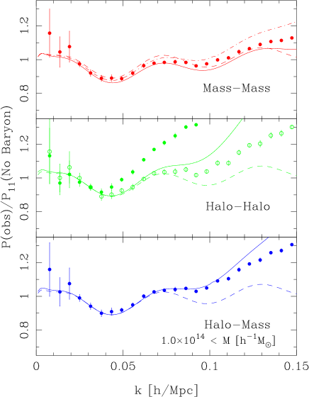
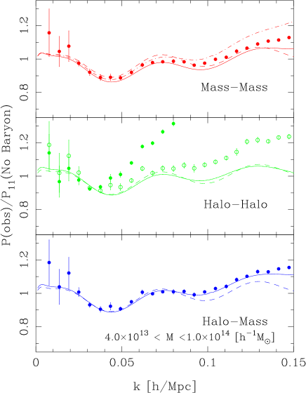
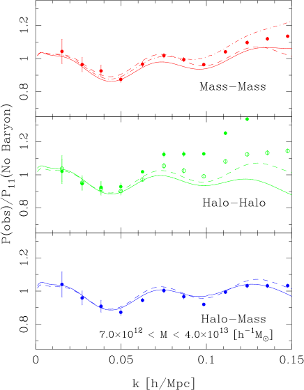
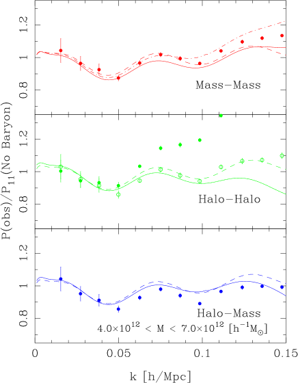
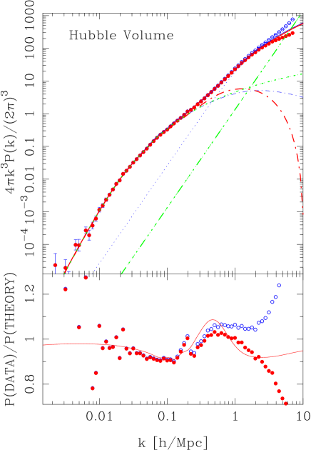
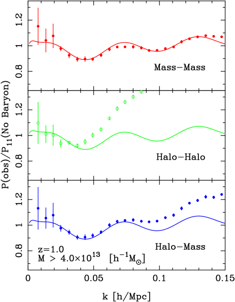
Figure 1 shows the three types of power spectra measured from the ensemble of simulations for each of the four bins in halo mass described in Table 1. The filled circles and associated error bars in the top, middle and bottom sections of each panel show , , and . The open circles show the result of applying a non-standard shot-noise correction to , which we describe in Appendix A.
To emphasize the non-linear evolution of the spectra and the BAOs in particular, we have divided each spectrum by a smooth linear theory spectrum, which we shall refer to as our ‘No Baryon’ model. This was constructed by performing a chi-squared fit of the cmbfast transfer function data to the smooth transfer function model of Bond & Efstathiou (1984),
| (12) |
The derived parameters are: , , , , .
To compare the halo spectra with the linear theory we require estimates of the halo bias on very large scales, which we measure as follows. We begin by assuming that the spectra can be written
| (13) |
where and denote the type of spectrum considered and where, for reasons that will later be apparent, we distinguish between the bias from and . Hence, the likelihood of obtaining an estimate of the power in the -bin is assumed to be an independent Gaussian with dispersion
| (14) |
Thus the combined likelihood of obtaining the data set can be written,
| (15) |
On maximizing the likelihood function, we find the following estimator for the halo bias matrix
| (16) |
We construct error estimates through further differentiation of the Gaussian likelihood function:
| (17) |
Lastly, since we observe scale-dependent non-linear effects in the matter power spectrum for , we only use modes with in the fitting of the amplitude matrix . Estimates of the large scale bias parameters and are presented in Table 2. 777The procedure was also performed separately for the no baryon model spectrum, this was done in order for ratios to be taken.
The dark matter power spectra in Fig. 1 show significant deviations away from linear theory prediction: at , there is a suppression of power relative to linear theory, whereas at there is an amplification. Perturbation theory studies Bernardeau et al. (2002) refer to the suppression effect (caused by tidal terms) as ‘pre-virialization’. Recently, this has been understood in much more detail as a result of the damping of linear features by nonlinearities, leading to an exponentially decaying propagator that measures the loss of memory of the density field to the initial conditions Crocce & Scoccimarro (2006a, b). Although the effect in the power is rather well-known and has been observed in recent numerical simulations of CDM spectraPercival et al. (2001); Smith et al. (2003); Cole et al. (2005); Springel et al. (2005), our results constitute a rather precise measurement of this effect, with realistic errors drawn from the ensemble. A complete assessment of the damping of linear features such as BAOs is done by studying the propagator Crocce & Scoccimarro (2006a, b) rather than the power spectrum. See Crocce & Scoccimarro (2006b) for further discussion on this.
The solid and dot-dashed lines show predictions based on halofit Smith et al. (2003) and on 1-Loop perturbation theory (PT). The PT results do well compared to the simulations on very large scales, but for they increasingly over-predict the power. We note also that PT appears to predict the pre-virialization feature in the simulations, adding additional support to the claim that requires non-linear corrections on the scales of interest. However, qualitatively, it under-predicts the magnitude of the effect. We note that halofit does reasonably well at capturing the behavior for , but it appears to under predict the measured data.
Before moving on to and , we think it is worth noting that the BAOs in on have been erased. The large-box LR measurements show that the third peak is gone, and the height of the second peak has dropped so that it appears more as a plateau. However, the behavior at appears unchanged.
Discreteness corrections for have been studied in some depthSmith et al. (2003). However, for , the appropriate correction is more complicated because haloes are rare, highly clustered, and spatially exclusive. In Appendix A we show that the standard Poisson shot noise correction for the cluster power spectrum results in negative power at high . This lead us to propose a new method for making the ‘shot-noise’ correction that accounts for exclusion, which we discuss therein. The open circles in the middle sections of each panel in Figure 1 show the result of this new correction. Filled circles show the uncorrected power, and stars show the standard correction —clearly, the choice of correction is crucial. Note that owing to the arbitrary normalization things for the standard shot noise method look better than they actually are. Unfortunately, the residual uncertainties in our new procedure prevent us from making strong statements about the scale dependence of halo-halo clustering.
Whilst the discreteness correction is troublesome for it is almost negligible for (the halo model arguments which follow allow us to quantify this). Our estimates of are shown in the bottom sections of the panels in Fig 1. Notice that the scale dependence of , is a strong function of halo mass. for the most massive haloes shows no deviations from linear theory until . However, the pre-virialization feature appears and gets enhanced as one goes to lower masses. Indeed, for our lowest mass bin, is sub-linear until .
This has important consequences for the BAOs. In the highest mass bin (top left panel), the oscillations in at have been erased. However, the first trough, at , is unaffected. For the next mass bin (top right panel), the first peak and trough are unmodified, and that the second peak is becoming noticeable. This trend continues as we decrease mass; there is even a hint of the third peak in the bottom panels. These measurements indicate that non-linear dynamics can erase oscillations on progressively larger scales as halo mass increases and that small displacements to the positions of the peaks and troughs may occur and that these will also be dependent on halo mass. If the locations of these peaks and troughs are to play an important role in constraining cosmological parameters, our measurements suggest that understanding and quantifying these displacements will be very important.
Before continuing, we comment on the possible explanation of these shifts through simple scatter from cosmic variance. We remark that it is certainly possible to reconcile some of the shifts in the peak positions through this. However, we draw attention to the fact that all of the points in the cross-power spectra of the low mass haloes are systematically lower than expected from the linear theory. We also re-iterate that the derived error bars are the errors on the means for 20 realizations. One caveat is that since the spectra are normalized by the very-large scale modes of the power spectrum, where cosmic variance errors are larger, we expect some small fluctuations in the relative amplitudes of the theory predictions as more data is acquired. Estimates of the error in the present LR simulations suggest changes of the order to be acceptable; and this increases to for the HR simulations. If the amplitudes for the theory curves are too low by , then some of these discrepancies may be alleviated. However, it is unquestionable that non-linear effects are present on these scales and we must therefore firmly accept that it is likely that these may cause some shifting of the harmonic series. Only a wider and expanded numerical study will be able to address and answer these questions more completely.
The solid lines in the middle and bottom sections of each panel show predictions from the analytic model described in the following sections. In all cases this model provides a better description than does linear theory.
| Bin 1 888See Table 1 for definition of bins. | 2.19 | 0.94 | -0.98 | 2.23 | 1.68 | -4.08 | |
|---|---|---|---|---|---|---|---|
| Bin 2 | 1.53 | -0.30 | 0.94 | 1.41 | 0.04 | -1.29 | |
| Bin 3 | 1.13 | -0.46 | 1.47 | 1.04 | -0.85 | 0.37 | |
| Bin 4 | 0.98 | -0.44 | 1.44 | 0.91 | -0.74 | 0.55 |
III.3 Scale dependence of the bias
Next, we examine the scale dependence of halo bias. We will consider
| (18) |
as well as
| (19) |
For any particular realization the wave modes of the halo and dark matter density fields are almost perfectly correlated. Because the first set of estimators are derived from taking the ratio of measured power spectra, they are insensitive to this source of cosmic variance. In this sense, the second set of estimators are non-optimal. However, they are the ones which will be used with real data, since is generally not observable.
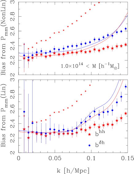
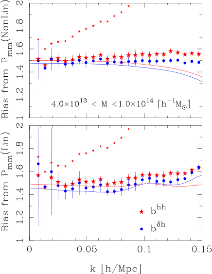
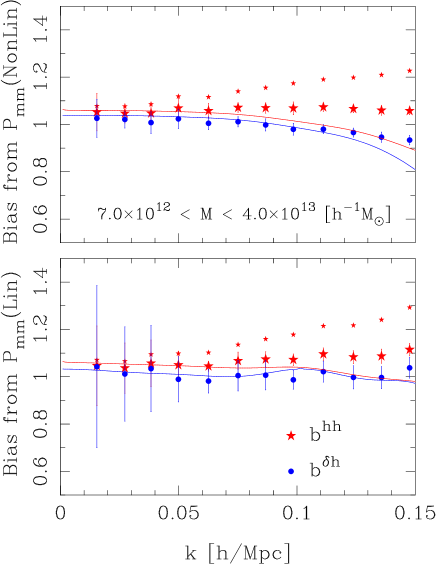
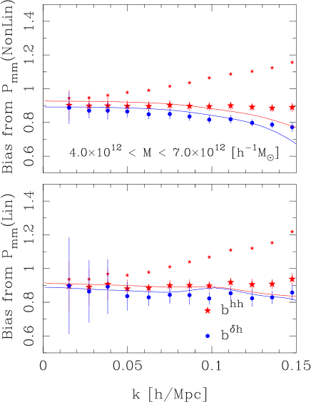
In Figure 2 we show the results of measuring these quantities for the same halo mass bins as in the previous section. The top and bottom parts of each panel show (18) and (19), respectively. The error bars, which were derived from the ensemble to ensemble variations, are significantly larger for (19) than for (18), as expected. The solid lines show the predictions from the new analytic model described in the next section.
For we show both the shot-noise corrected (large stars) and un-corrected (small stars) results. As was the case for the halo-halo power spectra, we see that this correction is important, so it must be known rather accurately. The estimators for are also shown (filled circles). Except for the highest mass bin, . Indeed, as we shall argue later, there are compelling theoretical reasons why the biases derived from and are not in fact the same, and that, one generally expects . However owing to the uncertainty regarding the shot noise correction, no firm statement can be drawn from the current data.
Two possible explanations why the highest mass halo bin appears to behave differently are: Firstly, if the shot noise correction to is too aggressive, we may have underestimated the true and therefore the bias. Alternatively, we have made no shot-noise correction to ; if one should be applied (we think this is unlikely, owing to the large number of dark matter particles), then our current estimate of may be biased high.
The estimators based on equation (19) show more scale dependence than those based on (18), especially for the two high mass bins. As noted by Guzik, Bernstein & Smith (2006), this is because the BAOs are erased on larger and larger scales as higher and higher mass haloes are considered. Thus on dividing the halo spectra by a linear theory BAO spectrum, we are in fact introducing scale dependence from the linear model.
For the highest mass haloes, is constant at , but it increases monotonically as increases. This is a direct consequence of the absence of pre-virialization in on intermediate scales and the rapid onset of non-linear power on smaller scales, compared to . The bias is flat for haloes with masses , suggesting that small clusters and group mass haloes are linearly biased tracers of the non-linear dark matter. The smallest two bins in halo mass show the reverse trend: the bias decreases at large , by compared to the approximately constant value at smaller .
IV Theoretical Model
We now describe a model for interpreting the trends seen in the previous section. Our discussion is based on the ‘halo-model’, which we briefly summarize below. See Cooray & Sheth (2003) for a more detailed review.
IV.1 The ‘Halo Model’ of large scale structure
The halo model may be described by the simple statement:
-
•
All dark matter in the Universe is contained within a distribution of CDM haloes, with masses drawn from some mass function and with the density profile of each halo being drawn from some universal stochastic profile.
The model attains its full potential when the second assumption is stated:
-
•
All galaxies exist only in isolated dark matter haloes, with more massive haloes hosting multiple galaxies.
In essence the model has been in existence for several decades Neyman & Scott (1952); Peebles (1974); McClelland & Silk (1977); White & Rees (1978); Scherrer & Bertschinger (1991); Mo & White (1996); Sheth & Jain (1997). However it was not until the advent of large numerical -body simulations and accurate characterization of halo phenomenology that its true value was realized. Namely, given an appropriate Halo Occupation Distribution (HOD – i.e., a prescription for the number and spatial distribution of galaxies within a halo) the model successfully reproduces the real-space form of the two-point correlation function of galaxies over a wide range of scales. It predicts subtle deviations from a power-law which have recently been seen in observations Zehavi et al. (2004) and provides a framework for describing the luminosity Yang et al. (2004); Zehavi et al. (2005) and environmental dependence of galaxy clustering Skibba et al (2006); Abbas & Sheth (2006). It also enables new tests of the CDM paradigm to be constructed Smith & Watts (2005); Smith, Watts & Sheth (2006).
IV.2 Power spectrum
In the model the density fields of haloes and dark matter may be written as a sums over haloes,
| (20) |
where distinguishes between haloes and dark matter and and are the total number of haloes and the number of haloes in some restricted range in mass. and are the mass and center of mass of the th halo and is the mass normalized density profile. Following Scherrer & Bertschinger (1991), the power spectra , and can be written as the sum of two terms:
| (21) |
The first term, , referred to as the ‘1-Halo’ term, describes the intra-clustering of dark matter particles within single haloes; the second, , referred to as the ‘2-Halo’ term, describes the clustering of particles in distinct haloes. They have the explicit forms:
| (22) | |||||
| (23) | |||||
where is the halo mass function, which gives the number density of haloes with masses in the range to , per unit mass. The matrix carves out the halo density field to be considered, e.g. for haloes with mass the matrix is
| (26) | |||||
where is the Heaviside Step Function. More complicated halo selections can easily be described through the notation. Lastly, is the power spectrum of halo centers with masses and . This function contains all of the information for the inter-clustering of haloes; precise knowledge of this term is required to make accurate predictions on large scales.
In principle, is a complicated function of , and . Initial formulations of the halo model (Seljak, 2000; Peacock & Smith, 2000; Ma & Fry, 2000; Scoccimarro et al., 2001) assumed that it could be well-approximated by
| (27) |
where all the scale dependence is in , which is taken from linear theory, and all the mass dependence is in the scale-independent bias parameter Mo & White (1996); Sheth & Tormen (1999). In this approximation, is a separable function of , and . As we show below, comparison with numerical simulations shows that this simple model over-predicts power on very large scales and provides insufficient power on intermediate scales. In both cases, this is about a ten percent effect.
This discrepancy is not unexpected (Sheth et al, 2001; Berlind & Weinberg, 2002; Yang, Mo & van den Bosch, 2003). A simple correction results from setting
| (28) |
where is the non-linear rather than the linear matter power spectrum, and, in addition, imposing an exclusion constraint:
| (29) |
where is the virial radius of the halo.
The success of this approach is demonstrated by comparing measured in the output of the Hubble Volume simulation Evrard et al. (2002) with the halo model calculation. The open and filled symbols in the top panel of Figure 3 show the measurement before and after subtracting a Poisson shot noise term (which is shown by the triple dot-dashed line.) The dot-short dash line shows the linear theory prediction, and the other two dot-dashed curves show two estimates of the 2-halo term: the one which drops more sharply at large is based on equation (28) and the other one is based on the original approximation of equation (27). Since equation (28) requires the use of a nonlinear power spectrum, we used the one provided by Smith et al. (2003).
The symbols in the bottom panel show the measurements divided by the halo model calculation which uses equation (27) for the 2-Halo term (i.e. the initial linear theory-based approximation). Notice how they drop below unity at . The solid line shows the halo model calculation which is based on equation (28)—it reproduces this pre-virialization feature well.
As an interesting aside, we note that the fitting formula halofit does very well at matching the pre-virialization feature. Whilst it is not apparent from the figure we also point out that the transfer function of the Hubble volume simulation does contain BAOs; thus, our results demonstrate that the fitting formula of Smith et al. (2003) appears to be accurate, for this data, for BAO models to roughly . In light of this, we note that the discrepancy between halofit and the mass power spectra from our smaller box HR simulations is somewhat puzzling. We highlight this issue for further study, one possible explanation is the difference in initial power spectra, on the other hand, also note that a calculation within the framework of Renormalized Perturbation Theory Crocce & Scoccimarro (2006a) suggests that even for these simulation volumes on expects small effects due to absence of coupling to large scales.
To fix the small discrepancies which remain, some authors have advocated making the halo bias factors scale dependent Tinker et al. (2005), but the implementation has been based on fitting formulae rather than fundamental theory. While equation (28) appears to fare better than the original approximation (27), as we will soon show, in going from (27) to (28), one is making the assumption that halo bias is linear even when the mass density field is not. If this is not the case then the method is incorrect. In addition, there is an unpleasant circularity in requiring prior knowledge of in order to predict .
IV.3 Halo bias: The non-linear local bias model
The discussion above makes clear that a rigorous treatment of the 2-Halo term is currently lacking. This term requires a description of how dark matter haloes cluster. Whereas current models seek to describe halo clustering as a biased version of dark matter clustering, the scale dependence of halo bias is still rather poorly understood Cole & Kaiser (1989); Mo & White (1996); Mo, Jing & White (1997); Catelan, Matarrese & Porciani (1998); Jing (1998); Sheth & Lemson (1999); Sheth & Tormen (1999); Jing (1999); Kravtsov & Klypin (1999); Hamana et al. (2001); Seljak & Warren (2004); Tinker et al. (2005). In the following sections we develop a model to understand its main properties. In particular, we will discuss a general non-linear, deterministic, local bias model for dark matter haloes. This model is exactly analogous to that derived for galaxy biasing by Fry & Gaztañaga (1993) and first applied to dark matter haloes by Mo, Jing & White (1997).
To begin, consider the density field of all haloes with masses in the range to , smoothed with some filter of scale . We now assume that this field can be related to the underlying dark matter field, smoothed with the same filter, through some deterministic mapping and that this mapping should apply independently of the precise position, , in the field: i.e.
| (30) |
where the sub-scripts on the function indicate that it depends on the mass of the haloes considered and the chosen filter scale. The filtered density field is
| (31) |
being some normalized filter. Taylor expanding about the point yields
| (32) |
We now assume that there is a certain filter scale above which is independent of both the scale considered and also the exact shape of the filter function. Hence,
| (33) |
where the bias coefficients are
| (34) |
The linear bias model has for all .
The bias coefficients from the Taylor series are not independent, but obey two constraints. The first arises from the fact that , which leads to
| (35) |
Thus, in general is non-vanishing and depends on the hierarchy of moments. This allows us to re-write equation (33) as
| (36) |
Nevertheless, we may remove from further consideration by transforming to the Fourier domain, where it only contributes to .
The second constraint states that a sum over all halo density fields weighted by halo mass and abundance must recover the dark matter density field Scoccimarro et al. (2001). This requires that
| (37) |
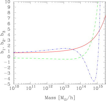
For CDM models whose initial density perturbations are Gaussian Random, the bias coefficients may either be derived directly through the ‘peak–background split’ argument Cole & Kaiser (1989); Mo & White (1996); Mo, Jing & White (1997); Sheth & Tormen (1999) or measured directly from -body simulations. Figure 4 shows the halo bias parameters up to third order, derived in the context of the Sheth-Tormen mass function; see Scoccimarro et al. (2001) for the analytic expressions. We compare these with measurements from our simulations in Appendix B.
A practical application of this method rests squarely upon our ability to truncate the Taylor series at some particular order. However, since the procedure that we have adopted for doing this requires some further knowledge, we shall reserve our discussion until Section V.2.
IV.4 HaloPT: Evolution of halo fields
We now evolve the halo density field as expressed by equation (33) into the non-linear regime via perturbation theory techniques. For a short discussion of these methods see Appendix C, and for a full and detailed review see Bernardeau et al. (2002). The main idea that we require from perturbation theory is that each Fourier mode of the density field may be expanded as a series,
| (38) |
where is the th order Eulerian perturbation and is the linear growth factor. Thus, on Fourier transforming the halo bias relation of equation (33), truncated at third order, and on inserting the PT expansion from above, we arrive at (keeping up to cubic terms)
| (39) | |||||
where . We next insert the solutions for each order of perturbation, which are presented in equation (86) of the Appendix, into equation (39). On re-arranging terms and collecting powers of , the mildly non-linear density field of dark matter haloes may be written as a PT series expansion of the dark matter density. This series is
| (40) | |||
| (41) |
where is the th order perturbation to the halo density field, and where the short-hand notation has been used. The functions are the Halo-PT kernels, symmetrized in all of their arguments. The first three may be written in terms of the dark matter PT kernels:
| (42) | |||
| (43) | |||
| (44) |
where . Thus equations (40) and (41) can be used to describe the mildly non-linear evolution of dark matter halo density fields to arbitrary order in the dark matter perturbation, and equations (42–44) make explicit the halo evolution up to 3rd order. Together, these ideas define our meaning of the term ‘Halo-PT’.
It is now apparent that halo clustering studies which assume a linear bias model and take the power spectrum to be the fully non-linear one, are effectively assuming that , with for . However, for CDM, the peak-background split argument informs us that this never happens, unless the density field itself is linear Cole & Kaiser (1989); Mo & White (1996); Mo, Jing & White (1997); Sheth & Tormen (1999); Scoccimarro et al. (2001). We must therefore conclude that extrapolating the linear bias relation into the weakly non-linear regime, without full consideration of the non-linearity of halo bias is incorrect.
V The 1-Loop Halo Model
V.1 Halo center power spectra
We now use the Halo-PT to calculate the power spectrum of halo centers in the mildly non-linear regime. We define the power spectrum of halo centers for haloes with masses and to be
| (45) |
On inserting the Halo-PT solutions for each order of the perturbation we find that can be written as the sum of three terms
| (46) | |||||
where
| (47) | |||
| (48) | |||
| (49) |
Here is equivalent to the linear theory power spectrum and
| (50) |
When these expressions are averaged over all halo masses, weighted by the respective cosmic abundances and , then the constraint equation (37) guarantees that they reduce to the standard ‘1-loop’ expression for the PT power spectrum of dark matter (Bernardeau et al., 2002):
| (51) |
Strictly speaking the 1-Loop power spectrum refers to , we shall break convention and use equation (51) to define what we mean. Explicit details of the 1-Loop expressions may be found in Appendix C.2.
The theory may be further developed by directly substituting the Halo-PT kernels, given by equations (42-44), into equations (47–49). A little algebra shows that
| (52) |
where
| (53) |
Before continuing, we point out and answer an important question that naturally arises at this junction: How does one compare the filtered theory with the unfiltered observations? We forward the proposition that the unfiltered nonlinear power spectrum can be recovered through the following simple operation:
| (54) |
This is unquestionably true for an observed non-linear field. It will therefore also be true for the correct theoretical model.
This rather lengthy expression may be more readily digested through the examination of two limiting cases. But first, notice the important fact that it is still a separable product of mass dependent terms and scale dependent terms.
When the two halo masses are identical, then
| (55) |
This expression is equivalent to evolving the non-linear, local, galaxy bias model Fry & Gaztañaga (1993) through Eulerian PT. This has been explored by Heavens, Matarrese & Verde (1998) and Taruya (2000).
Secondly, consider the case where we integrate over one of the halo masses, say , weighting by and its abundance . Equation (37) again insures that all terms involving and vanish, and so the resulting expression is the 1-Loop correction to the halo center–dark matter cross power spectrum:
| (56) | |||||
Inspection of these two limiting cases reveals three remarkable features:
-
•
Firstly, if the non-linear bias parameters and are non-vanishing then the bias on large scales is not .
-
•
Secondly, the halo-halo spectrum has a term that corresponds to constant power on very large scales, whereas the cross spectrum does not.
Both of these points were independently noted by Heavens, Matarrese & Verde (1998) and Taruya (2000), but for the case of non-linear galaxy biasing (also see Scherrer & Weinberg (1998)).
-
•
Thirdly, the large scale bias derived from the halo-dark matter cross power spectrum is not , nor is it given by the bias derived from the halo-halo power spectrum.
These expressions make the first point noted above trivially obvious: The large scale bias is modulated by the Halo-PT correction terms, and these depend on the non-linear bias parameters and and also on the filtered variance of fluctuations.
The second point noted above originates specifically from the quadratic non-linear bias terms found in equations (57) and (58), e.g. terms containing and . For a linear power spectrum that obeys the limit , these expressions reduce to the constant
| (60) |
This term was discussed in great detail for the case of galaxy biasing by Heavens, Matarrese & Verde (1998).
The third point noted above can be understood by constructing the linear bias, e.g. dividing equations (59) and (58) by . On squaring the bias recovered from (59) and subtracting it from the bias from (58), we find
| (61) |
We now see that, because approaches a constant on very large scales, on dividing through by the bias function diverges at the origin as diverges.
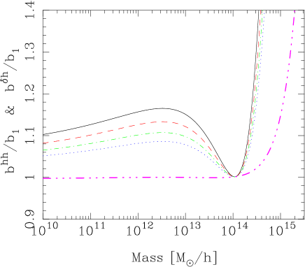
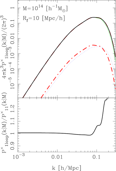
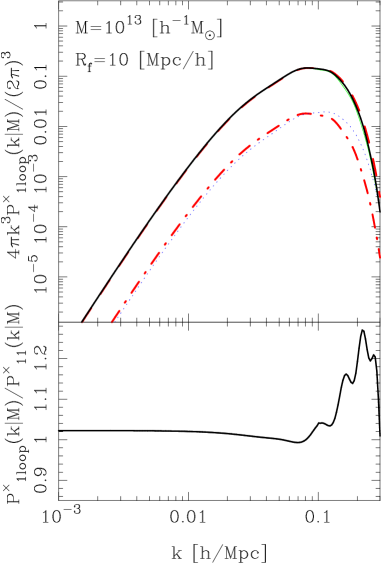
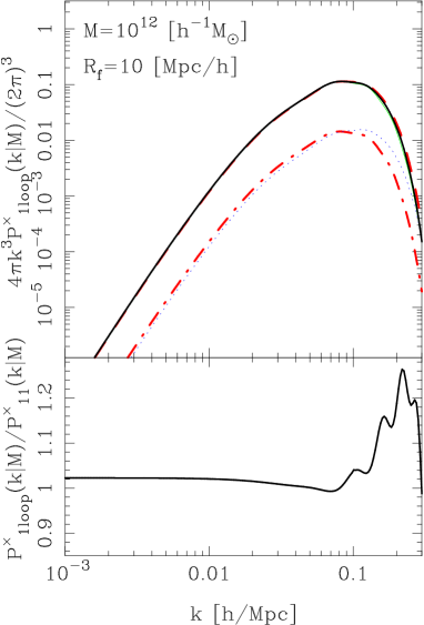
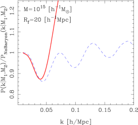
Figure 5 shows our expressions for and (from equations 57 and 58). In this particular case, we assume the nonlinear bias parameters derived from the Sheth-Tormen mass function by Scoccimarro et al. (2001). We use a Gaussian filter, for which . For and for our fiducial cosmology, we find . To inspect the differences more closely, we take the ratio of the predictions with respect to the tree-level theory, e.g. . The figure demonstrates two of the points raised above. Firstly the large scale bias is not simply : halo-halo bias (solid through to dotted curves) does not converge as one considers larger and larger scales; however bias from the cross power spectrum is very close to linear for all except the most massive haloes, where and are very strongly rising functions (see Fig. 4). Secondly, it is now obvious that and are not the same. Note also that the magnitude of the expected scale dependence: the bias varies by at most five percent when is changed by an order of magnitude. The mass dependence of shown in Fig. 5 is simply driven by that of (again see Fig. 4). As halo mass increases the bias slowly increases until it reaches a maximum at . It then decreases to after which it shoots up dramatically for larger masses.
V.2 Convergence of the power spectrum
We now return to the issue of truncation and applicability of the Taylor series expansion of the halo field. A first requirement for the Taylor series to converge after a finite number of terms is that the filter scale be large enough so that the rms dark matter fluctuations be much less than unity: . Consider the case where is very large and convergence occurs at first order, we then have: . As the filter scale is slowly decreased the rms fluctuations in increase and a larger and larger number of terms are required to accurately map the underlying bias function. Finally, as all terms in the series are required. At this point the method has no merit.
Since a robust criterion for truncation is out of reach at present, we propose an ad-hoc criterion for convergence that must plausibly be obeyed, that is
| (62) |
In Appendix B we shall also discuss an empirical method for testing convergence.
V.3 Returning to the halo model
We now translate these ideas back into the language of the halo model. To begin, we shall restrict our attention to the halo model in the large scale limit, more precisely we consider scales where . Since the Fourier transform of the mass normalized profile may be written
| (63) |
our large scale condition simply becomes . In the above equation we have, for convenience, assumed spherical density profiles. If halo mass and virial radius are related through , then for the largest collapsed objects in the Universe , and the above condition translates to the inequality . If we assume an NFW density profile Navarro, Frenk & White (1997) with concentration parameter , then for , we find that . We therefore assume that this is an excellent approximation over the scales that we are interested in.
Hence for scales , our equations (22) and (23), at the 1-Loop level in Halo-PT, now take the forms:
| (64) | |||||
| (65) | |||||
where we have explicitly included a filter on the 1-Halo term. (Recall that the halo center power spectrum in the 2-Halo term already includes such a filter.)
We now see that, because the are the only mass dependent functions, on insertion of equation (52) into equation (65) the integrals over mass may be immediately computed. Thus,
| (66) |
where is equivalent to equation (52), except that we have replaced all of the mass dependent bias parameters by the average ones: i.e.
| (67) |
We note that if we wish to weight by halo number density rather than mass density then we simply remove the mass weighting in the numerator and denominator of .
VI Evaluation of the theory
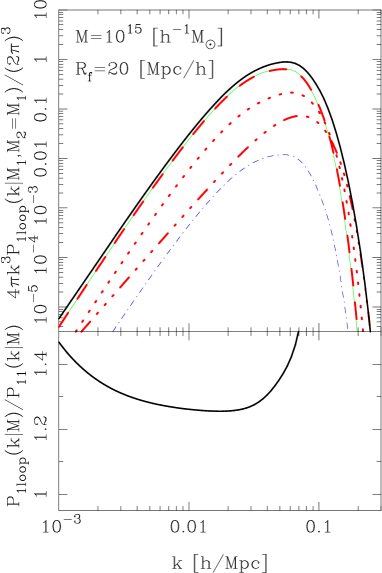
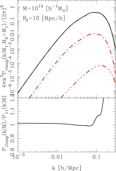
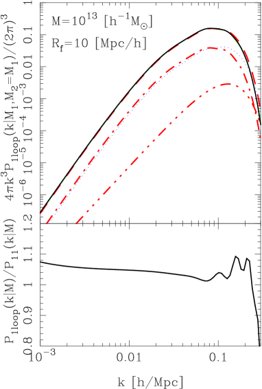
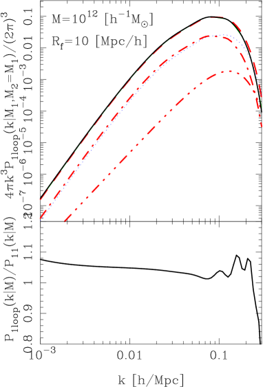
In this section we present the results from the direct computation of the 1-Loop halo center expressions for and , as given by equations (55) and (56), respectively. This section is almost entirely pedagogical; we urge those who are only interested in the direct comparison with the numerical work to press on to Section VII.
Recall that it is necessary to adopt some filter scale . We have studied two choices: and for which the linear theory, Gaussian filtered, variances are and , respectively. The larger smoothing scale is required for the more massive haloes.
VI.1 Halo–dark matter cross power spectra
In Figure 6 we show the predictions for the scale dependence of at the 1-Loop level, as a function of wave number. The different panels show results for different halo masses and smoothing scales. In all four panels, we see that, as expected, there is a small (few percent) positive offset from the linear theory bias value . The largest offset occurs for the cluster mass haloes, but here it may be the case that, owing to the bias being large, the filter scale that we have adopted for these objects may still be too small for adequate convergence. We also note that the offset for the haloes is negligible. This can be attributed to the fact that (see Fig. 4 ). For the lower mass haloes the offsets are roughly in excess of linear.
Considering the predictions for the highest mass haloes, we see that the spectrum is scale independent up to , where the non-linear amplification from the term becomes dominant. For this case, the absence of the pre-virialization feature may be understood as follows: Firstly, we note that and are positive, whereas is negative. However, since is an order of magnitude smaller than the others, it plays no significant part in determining the shape of the spectrum. The term in the 1-Loop power spectrum, which is the main cause of the pre-virialization feature, is thus overwhelmed by the action of the quadratic bias term. This suggests that should be scale independent up to .
Next, we collectively consider the predictions for the lower mass haloes, as they show many similar traits. Firstly, we find that when , then the ratios of the 1-Loop to tree level (or linear) spectra are flat. However, for , significant scale dependence is apparent: the pre-virialization feature is present and it appears to become stronger as halo mass decreases. On smaller scales still, the non-linear boost from the term amplifies the power spectrum and breaks all scale independence. Interestingly, the onset of is pushed to smaller scales as halo mass decreases. These effects can be understood as follows. For these objects and are positive, whereas is negative. On large scales, we see that and are nearly equivalent, but is slightly dominant, and this results in a small positive correction. Whereas on smaller scales this trend reverses and becomes dominant. The overall correction is then negative and this leads to the enhanced pre-virialization feature and delay of the onset of .
It is also interesting to note the imprint of the BAO features in the ratios of the power spectra. The strength of the signal appears to depend on halo mass and increases as halo mass decreases. As we discussed in Section III.3, this can be attributed to the fact that non-linear evolution suppresses BAOs on small scales, and on taking the ratio with a linear theory spectrum, we are artificially introducing oscillations.
VI.2 Halo-Halo power spectra
In Figure 7 we show the predictions for the scale dependence of , at the 1-Loop level, as a function of wavenumber. The four panels show results for haloes with masses in the same range as Figure 6. Again, upper panels show the contributions from each of the Halo-PT terms in equation (55), and where the sign of each contribution is distinguished through line thickness/color. Sub-panels are as before.
Some obvious similarities exist between the auto-halo spectra and the cross spectra. In particular: the large scale bias is not given by ; the highest mass halo spectrum shows no sign of the pre-virialization power decrement; the non-linear boost occurs increasingly at smaller scales as halo mass decreases; with the exception of the highest mass haloes, the ratio of the 1-Loop spectra to the tree level spectra have BAOs imprinted. These effects may all be understood through the explanations from the previous sub-section.
We also notice some important differences between and . Firstly, the addition of the quadratic non-linear bias term, , modifies the results on the largest scales. As was discussed in Section V, becomes a white-noise power spectrum as , unless . In the figure, the contributions from this term are denoted by the triple dot dash lines. On considering all four panels and paying special attention to the ratios, we see that, with the exception of the case , there is an upturn in power on scales . For the haloes this effect is not found, this owes to the fact that (see Fig 4).
Secondly, we note that on smaller scales the effect of the term is to boost the power across all scales. Thus the pre-virialization power decrement is no longer a decrement relative to the linear theory. However, relative to the power measured on say , there is a very real decrement. Moreover, the -dependence of the terms multiplying will make the decrement appear larger than we would expect from the non-linear matter spectrum.
VI.3 Non-linear evolution of BAOs
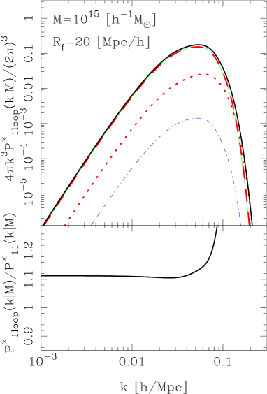
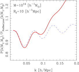
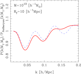
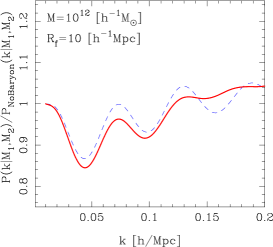
We now briefly consider how mode-mode coupling and non-linear biasing affect the evolution of the BAOs. Figure 8 compares the 1-Loop predictions for with the linear theory predictions. We again consider the set of halo masses: , and, to emphasize the evolution of the BAO features, we have taken the ratio of each spectrum with the ‘No Baryon’ model of equation (12). In addition, because we are purely interested in the scale dependence, we re-normalize all ratios to unity at .
The top left panel shows results for the highest mass haloes: all but the first of the BAO troughs has been removed through non-linear evolution. This is a much more aggressive non-linear evolution than one expects from considerations of the dark matter alone. Secondly, the trough appears to have been displaced towards lower frequencies. These effects arise because both the quadratic bias and terms are positive, and so dominate over the negative and terms. This fact, coupled with the injection of power from , means that the non-linear boost occurs at . Thus, the overall effect on the halo spectrum is to shift the first trough to smaller .
All the spectra of the lower mass haloes display a pre-virialization feature, the strength of which increases as halo mass decreases. In addition, the number of peaks and troughs which remain in the evolved spectra increases as halo mass decreases, because the strong non-linear amplification from the term is delayed by the negative corrections. However, in contrast to the high mass haloes, for the low mass haloes the first acoustic trough is shifted towards larger because, when , then the negative correction from the term is dominant and so subtracts power from the higher frequency side of the oscillation. This acts to shift the overall pattern to higher frequencies.
VII Comparison with simulations
In this Section, we compare the predictions from the theoretical model with the results from the numerical simulations presented in Section III.
VII.1 Halo center power spectra re-visited
Returning to our analysis of Figure 1, We are now in a position to comment on the success of the Halo-PT model in comparison to the numerical simulations. The analytic model was evaluated using the semi-empirical bias parameters that were determined as described in Appendix B. Since here we are concerned purely with the scale-dependence of the spectra and not their overall amplitude, we allowed the very large scale normalizations to be considered as free parameters. These were fit-for in exactly the same way as was done for the linear theory models in equation (13). Whilst this re-scaling would not be necessary if the bias parameters that we were adopting were precise and accurate, since we have not been able to establish this in a robust manner we feel that this approach is acceptable, given that it has been equally applied to the linear theory. Moreover, this is the method of analyzing real data.
These predictions are shown as the solid lines in Figure 1. Comparison with the measured , shows that the model and the shot-noise corrected data show reasonable correspondence over scales . On smaller scales the match is poor. However, the uncertainty in the shot-noise correction makes it very difficult to draw firm conclusions.
Considering , we find that the analytic model is in good agreement with the simulations over a much larger range of scales. The model correctly captures the mass dependence of the pre-virialization feature – low mass haloes show greater loss of memory to the initial density fluctuations. The shifting of the nonlinear boost to smaller scales as halo mass decreases is also matched rather well.
To assess whether is a better fit to the simulation data than is linear theory, we have performed a likelihood ratio test, assuming that the likelihood functions are Gaussian. In this case, a necessary statistic for model selection is for
| (68) |
where the subscript ‘max’ refers to the parameter choices in the models that maximize the likelihood. Restricting the information to be , we find, going from low to high mass haloes, that , respectively.
VII.2 Halo bias re-visited
We now examine how well the Halo-PT model does at matching the nonlinear scale dependent bias of the halo centers as measured in the numerical simulations (Figure 2). The top section of each panel shows that the analytic model (solid blue and red lines correspond to and , respectively) captures, qualitatively, the scale dependence of the bias. The model shows a bias that increases with for the high mass haloes but decreases with for lower masses. However, there are some notable discrepancies: The model under predicts and then over shoots the measured relationship for the most massive haloes; for the next bin in halo mass (top-right panel), the measured bias is flat, whereas the model predicts a down turn after ; the model fares better in the two lowest mass bins, but the down-turn at high is not seen in the data. However, we must stress that, with the exception of the haloes, the model out-performs linear theory, which would predict constant bias on all scales.
Having extolled the virtues of our model we now draw attention to its short-comings. Whilst the predictions provide a good match to the halo power spectra, they do not simultaneously provide a good match to the scale dependence of the bias. If we re-consider our measurements of the non-linear matter power spectrum (upper sections in Fig 1) , we see that the 1-Loop model (dot-dash lines) over predicts the LR simulations on scales and the HR simulations on scales . It is therefore unlikely that the model as presented here can be made to work precisely .
VIII Galaxy power spectrum
How does the scale dependence of the bias depend on galaxy type? The answer has important consequences for future galaxy surveys that will measure the clustering of specific sub-classes of objects. We may address this question using the halo model by changing the mass weighting in the integrals to:
| (69) |
where and are the first two factorial moments of the halo occupation probability function , which gives the probability for a halo of mass to host galaxies. Use of the factorial moments of subtracts off a term corresponding to the self-correlation of galaxies e.g. . This corresponds to the Poisson shot noise term in Fourier space. Secondly, the mean density profile of dark matter is changed to the mean density profile of galaxies in the halo: . Following the discussion in Section V.3, it is a very good approximation to set when . Thirdly, the constant pre-factors transform as , where
| (70) |
And finally, the galaxy bias parameters are
| (71) |
These changes in equations (64) and (65) yield the 1-Loop halo-model prediction for the galaxy power spectrum. Explicitly:
| (72) | |||||
| (73) | |||||
where again we have explicitly included a filter function on the 1-Halo term. On inserting our expression for from equation (55) into the 2-Halo term, and again noticing that in the large scale limit the mass integrals may be performed directly, we find:
| (74) | |||||
The resulting expression for the galaxy power spectrum is identical to that given by Heavens, Matarrese & Verde (1998); Taruya (2000), with one important difference—we include the large scale constant power originating from .
To study the expected differences between red and blue galaxies, we use the parametric forms for measured by Sheth & Diaferio (2001) in the semi-analytic models of Kauffmann et al. (1999):
| (75) |
The blue galaxy parameters are: ; for haloes with masses in the range then , for larger mass haloes . The red galaxy parameters are: ; for haloes with masses greater than the cut-off mass . For the second moment of the HOD we follow the model of Kravtsov et al. Kravtsov et al. (2004), so that . This makes sub-Poissonian as suggested from the observations Peacock & Smith (2000); Yang, Mo & van den Bosch (2003); Zehavi et al. (2005) and the semi-analytic models Benson et al. (2000); Sheth & Diaferio (2001); Scoccimarro et al. (2001); Berlind et al. (2003); Zheng et al (2005); and secondly, this choice allows the first moment alone to fully specify the hierarchy of moments.
In practice, we use the models above but impose a lower mass cutoff of . This yields , , and . (This estimate of agrees with the observational determinations of similar galaxies from the PSCz survey Feldman et al. (2001).) These values are easily understood by noting how depends on halo mass (e.g. Figure 4), the weightings given in equation (75), and recalling that the halo mass function declines exponentially at . Notice that the red galaxy bias parameters are all positive, whereas for the blue galaxies is negative. Therefore, while we expect to see a pre-virialization feature in , we do not for the red galaxies.
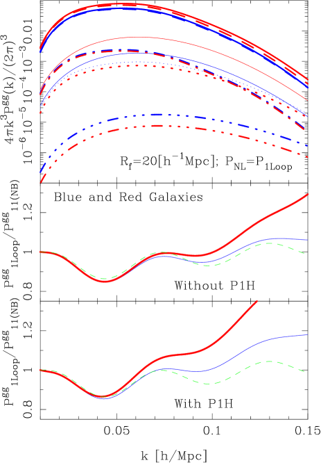
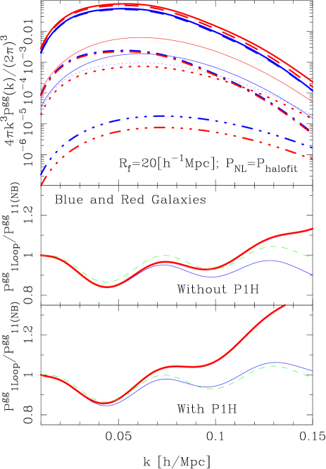
The left panel of Figure 9 shows the power spectrum of blue and red galaxies evaluated using the 1-Loop Halo model. The top section shows the individual contributions from all the linear and nonlinear terms. Note that, for the blue galaxies the non-linear correction terms (blue dotted lines) and (blue dot-dash lines) are roughly the same order of magnitude as the 1-Halo term (thin blue line). However, for the red galaxies, the 1-Halo term (thin red line) dominates over the non-linear bias corrections by factors of a few. For both populations the quadratic bias terms (triple-dot-dash lines) appear to be negligible.
The middle section of the left hand panel shows the ratios of the 1-Loop with the No-Baryon linear model (from equation 12). Again, since we are primarily interested in the scale dependence of the bias, we re-normalize all curves to be unity at . As expected, the red galaxy power spectrum appears to trace the linear theory matter fluctuations (green dash line) very well when . The non-linear boost breaks this accordance at larger . However, for the blue galaxies, the scale dependence is more complicated, having an increased pre-virialization feature and a delayed nonlinear boost. We also note that, for the red galaxies, the second and third BAOs have been almost completely suppressed, whereas only the third peak has been removed for the blue galaxies. The peaks and troughs, however, appear to be in the right places.
So far, we have neglected the contribution from the constant power 1-Halo term. In the bottom section of the panel we now take this into account and show ratioed to the No-Baryon model. For the red galaxies, the agreement between the predictions and the linear theory that was noticed before is now broken on much larger scales, . The trough of the first BAO has been shifted slightly to smaller and the non-linear boost occurs at a larger scale. Because the 1-Halo term is about 5 times smaller for the blue galaxies, the modifications are not as severe. The addition of this term offsets the suppression of power caused by the negative term and the blue galaxies now appear to trace the linear theory on scales quite well. At larger the linear spectrum is a poor match to the predictions. We also note that the BAOs are further suppressed and the second trough has been shifted to lower frequencies.
Because does not provide a very accurate model for the true non-linear power spectrum, we have studied the effect of exchanging for the halofit Smith et al. (2003) power spectrum. The results are shown in the right hand panel of Figure 9. Although the predictions are qualitatively very similar, halofit predicts enhanced pre-virialization and smaller non-linear boosts. In the middle panel, where the 1-Halo term is not included, we see that the red and blue galaxies do not match the linear theory as well on large scales. In particular the blue galaxy power is suppressed on all scales except the largest. We also see that the BAOs have been better preserved. Although there are slight shifts in the positions of the second trough and third peak. However, the bottom panel shows that once the 1-Halo term has been included, the red galaxy predictions are almost as before. The blue galaxies still show a reasonably strong pre-virialization feature, but, because of the weak nonlinear boost, they match the linear theory rather well over nearly all the scales considered.
We note that this modification is not entirely self-consistent and as such is not meant to be blindly trusted, since the non-linear bias terms are still derived from the 1-Loop Halo-PT. However, we use this operation to highlight that a more advanced understanding of the non-linear power spectrum does change the results quantitatively. This implies that a more advanced model of the scale dependence of the bias will also further modify and improve the predictions.
IX Scale dependent bias at
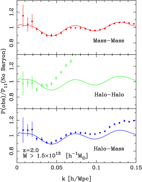
We have shown that the BAO harmonic series in the power spectrum at is affected by nonlinear effects from bias and gravitational evolution. Although naively one might expect that at higher redshift nonlinear effects are less important, this is not necessarily so. First, one must pick a criterion for how to compare things at different redshifts. A natural choice is to use objects of the same number density. In this case, as it is well-known, at higher redshifts objects of the same number density are more biased, leading to stronger nonlinear bias effects, even though the dark matter has less nonlinear evolution. Therefore, overall it is not clear a priori whether the situation improves or not. Figure 10 shows the halo power spectra at and measured from our 8 LR simulations, where the halo samples were harvested so that they would have the same fixed comoving number density as the Bin 1 sample at (see from Table 1). The power spectra analysis was identical to that as described in Section III. This figure clearly demonstrates that the non-linear bias effects that are present at (Fig. 1), remain present in the high redshift halo samples. In light of this, we anticipate that low mass halo samples at higher redshift, constructed so that , will likewise show enhanced pre-virialization ( is defined to be the halo mass at which ). We reserve further details of this issue for future work.
X Conclusions
In this paper we have explored in detail, through both numerical and analytic means, the scale dependence of the nonlinear dark matter, halo and galaxy power spectra on very large scales . For our numerical work we used and ensemble of 20 simulations in boxes of side and 8 simulations in boxes of side Gpc. Each simulation contained more than 134 million particles. We have found that:
-
•
The non-linear matter power spectrum is suppressed relative to the linear theory by on scales between at the 2- level.
-
•
The halo-dark matter cross power spectrum shows clearly that the bias of halo centers is non-linear on very large scales. The form of the non-linearity depends strongly on halo mass: for high mass haloes no pre-virialization suppression is seen; whereas there is an apparent suppression of power relative to linear theory for lower mass haloes.
-
•
To make robust statements concerning their large scale clustering of haloes, it is essential to characterize the shot noise correction to high precision. For high mass haloes this correction is sub-Poissonian, so the simple and widely used model must be inappropriate. Halo exclusion effects lead to a plausible explanation for this phenomenon, which we used to motivate an alternate correction. However further work is required to establish this robustly. In addition the true answer may need to take into account the way in which haloes are identified in simulations.
-
•
The large-scale bias of is not expected to be the same as that of due to nonlinear deterministic bias; this complicates studies of stochastic bias. The difficulty of performing the halo-halo shot noise correction means we are unable to make a strong statement about the non-equivalence of and .
-
•
As wavenumber increases, low mass haloes are increasingly anti-biased and high mass haloes are increasingly positively biased. Therefore, the non-linear scale dependence of halo bias is not simply due to the nonlinear evolution of the matter fluctuations.
-
•
Baryon acoustic oscillation features in the power spectrum are erased on progressively larger scales as halo mass is increased. In addition, small shifts in the positions of the higher order peaks and troughs occur which depend on halo mass.
In the second half of this paper we developed a ‘physical model’ to explain and reproduce these results. The model was constructed within the framework of the halo model and we focused our attention on the clustering of the halo centers. The halo-halo clustering term was carefully propagated into the non-linear regime using ‘1-loop’ perturbation theory and a non-linear halo bias model. Our model can be summarized as follows: The density field of haloes was assumed to be a function of the local dark matter density field. Under the condition of small fluctuations, it was then expanded as a Taylor series in the dark matter density with non-linear bias coefficients Fry & Gaztañaga (1993). The density field was then evolved under 3rd order Eulerian perturbation theory and this provided the 3rd order Eulerian perturbed halo density field. We then used the model to derive the halo-halo and halo-dark matter cross power spectra up to the 1-Loop level. This lead to the following conclusions:
-
•
For non-vanishing, the effective bias on very, very large scales for the halo spectra is not simply , but also depends on , and the variance of fluctuations on scale . The halo center power spectrum contains a term that corresponds to constant power on very large scales. This implies that as , halo bias should diverge as . The halo-dark matter cross power spectrum does not exhibit this behavior. The predicted bias from this statistic approaches a constant value on large scales.
-
•
When evaluated for a realistic cosmological model, with non-linear bias parameters taken from the Sheth-Tormen mass function, the theory is in broad agreement with numerical simulations for a wide range of halo masses.
-
•
The non-linear evolution of the BAOs was also examined. The model shows that non-linear bias and non-linear mode-mode coupling increasingly damp the BAOs as halo mass is increased. In addition, the positions of the peaks and troughs can be shifted by small amounts which depend on halo mass.
Using the ensemble of simulations we constructed scatter plots of the halo versus dark matter over densities, contained in top-hat spheres of size (see Appendix B). From these, it was shown that for filter scales the bias was indeed non-linear, and that, whilst the scatter increased as decreased, the mean of the relationship did not change until . We also examined whether the nonlinear bias parameters derived from the Sheth & Tormen mass function Sheth & Tormen (1999); Scoccimarro et al. (2001) provided a reasonable match to the empirical halo bias.
Using semi-empirical bias parameters as inputs for the analytic model it was shown that the model well reproduced the scale dependence of the halo-dark matter cross power spectra in the simulations, and for all bins in halo mass. However, it was only qualitatively able to reproduce the scale dependence of the non-linear halo bias.
The 1-Loop halo center power spectrum was then inserted into the halo model framework and defined the ‘1-Loop Halo Model’. This was used to predict the scale dependence of blue and red galaxy power spectra. Plausible models for the Blue and Red Galaxy HODs were used and the results showed complicated scale dependence.
Significant work still remains to be performed for this analytic approach to be sharpened into a tool for precision cosmology. Some possible improvements are: exchanging the 1-Loop matter power spectrum for an accurate analytic fitting formula i.e. after the fashion of halofit, but designed purely for large scales; an application of the new re-normalized perturbation theory techniques Crocce & Scoccimarro (2006a, b); Mc Donald (2006) coupled with the non-linear bias model should certainly produce better results.
The analytic and numerical results that we have developed here are concerned purely with the clustering in real space. In a subsequent paper we shall extend our analysis to explore the more realistic situation of the scale dependence of dark matter, halo and galaxy power spectra in redshift space.
When this paper was nearing completion, a preprint appeared Mc Donald (2006) with similar calculations of how nonlinear bias changes the power spectrum.
Acknowledgements
RES would like to thank Peter Schneider for a very thought provoking discussion that has led to the current paper. We thank Jacek Guzik, Gary Bernstein, Bhuvnesh Jain and Laura Marian for many useful discussions during this work. We would also like to thank Pat McDonald, Daniel Eisenstein, Eiichiro Komatsu and Martin White for useful comments on the draft. RES thanks Joerg Colberg and the Virgo Consortium for providing access to the Hubble Volume and the VLS simulations. RES thanks CCPP and NYU for their kind hospitality during part of this research. RS would like to thank M. Manera for useful discussions on halo exclusion. RKS would like to thank Martin White for many illuminating discussions and the Aspen Center for Physics. We thank M. Crocce and S. Pueblas for help regarding the numerical simulations used here. RES and RKS both acknowledge support from the National Science Foundation under Grant No. 0520647. RS is partially supported by NSF AST-0607747 and NASA NNG06GH21G.
.1 Poisson model
It is necessary to correct the measured dark matter power spectra for shot-noise errors. These arise through approximating the continuous CDM fluid by a point process. If the discretization of the density field obeys a Poisson process, i.e., dark matter particles are placed with probability , then the ‘discreteness’ correction is Peebles (1980):
| (76) |
Since the number of particles in our simulations is large, , this correction, on the scales of interest, is insignificant, e.g. . However, one must also correct for discreteness. If the dark matter haloes are also regarded as a Poisson sampling of the smoothed halo density field, then the correction will be the same but using the appropriate number density . In Figure 11 we show the effect of this standard correction on our halo power spectra and we plot the ensemble of the shot-noise corrected halo power. The negative power values that result at high demonstrate that this model must not be exactly correct and therefore for accurate measurements it must be modified in some way. We now discuss a possible explanation for this and propose a new shot correction.
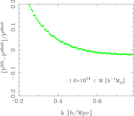
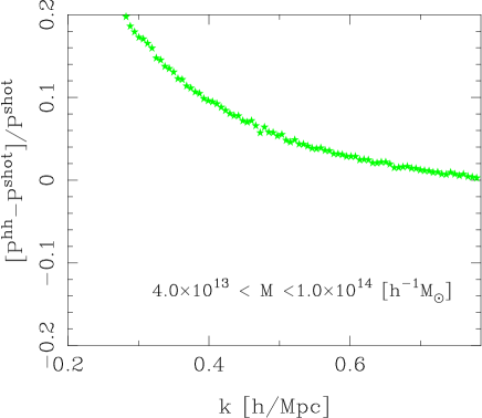
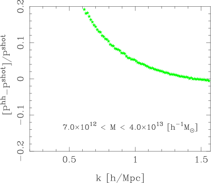
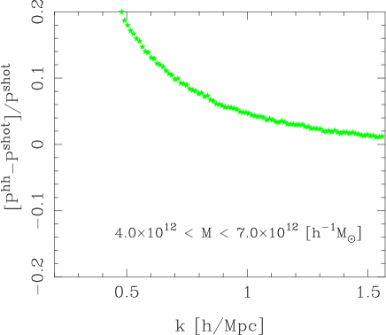
Appendix A Halo discreteness corrections
A.1 Halo exclusion effects
As we have seen Poisson sampling must not be exact for haloes, particularly those of large mass. A possible reason is that by using a friends of friends algorithm, one is automatically imposing that haloes are never separated by distances smaller than about the sum of their radii, else they would have been linked as a bigger halo. As a result of this exclusion effect, the two-point correlation function of haloes drops dramatically from a value at to for , where is the exclusion radius. This sharp drop of has an impact on the large-scale power spectrum, as we now show.
Absent exclusion, the power spectrum would have been
| (77) |
However, exclusion effects mean that
| (78) |
where with the Fourier transform of a top-hat window in real space. Hence, the difference in power due to exclusion is
| (79) |
To estimate this, we must model at scales smaller than the exclusion imposed by the friends of friends definition of a halo. We do so simply by approximating by a power-law obtained from fitting to the measurements, where is the exclusion scale. In this approximation
| (80) |
where, in the large-scale approximation ,
| (81) |
Setting gives in the same limit. Thus, we see that exclusion makes the halo power spectrum smaller by the amount given by Eq. (80). In contrast, Poisson shot noise makes the power larger by . If Poisson noise is subtracted from halo power spectra in simulations, then the result becomes negative at high . So it may be that adding back the power lost to exclusion will make the power positive again. This is our procedure. Note that the noise in Eq. (80) is not white.
As a final note we reemphasize that all of these troubling issues may, to a certain extent, be neatly side stepped, if we measure the halo-dark matter cross power spectrum. The clear advantage of this approach is that the ‘shot-noise’ is dramatically reduced (there are many more particles than haloes) and exclusion no longer plays a role.
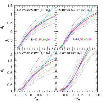
Appendix B Measuring the non-linear bias parameters
The accuracy of 1-Loop Halo PT depends on the accuracy of the halo bias parameters , and . Figure 4 shows these parameters derived from the conditional Sheth & Tormen mass function Scoccimarro et al. (2001). There are a number of ways to test the accuracy of the bias parameters. The most direct is to smooth the halo and mass fields with a filter of scale , and to then plot versus in the smoothed fields (e.g. Sheth & Lemson (1999); Casas-Miranda et al. (2002)). From the resulting scatter plot, one then directly fits for the parameters up to some order, subject to the constraint that .
Figure 12 shows such scatter plots for the four bins in halo mass described earlier (Table 1). In all cases, unlike elsewhere in the paper, the fields were filtered with a ‘top-hat’ window function. Solid blue, red, green and magenta lines show results for four filter scales . The upper and lower dotted lines show the errors about the mean relation (solid lines). (Smoothing with a Gaussian filter instead does not significantly change the mean, but does slightly change the scatter around the mean relation.) The figure shows that, above a certain scale, defines a universal curve which is independent of ; it is this curve which the bias coefficients are supposed to describe. The figure also shows that the scatter around this mean curve decreases as increases. The assumption that bias is deterministic is equivalent to assuming that this scatter, this stochasticity, is negligible. Clearly, this is a reasonable approximation only for large smoothing scales , and must be bigger for the rarer, more massive haloes before the bias can be called deterministic.
The main problem with this approach is that, when is large, then the distribution of becomes sharply peaked about its mean value (zero!), so estimating the higher order bias coefficients becomes difficult—only the linear bias term can be reliably measured. In effect, determination of the bias coefficients corresponds to fitting a polynomial to these mean curves, and the best-fitting coefficients will be correlated. The results of this exercise are tabulated in 2, which also shows the values of predicted from the Sheth-Tormen mass function. Some of the discrepancy is a consequence of the fact that the Sheth-Tormen mass function under-predicts the abundance of high mass haloes in the HR and LR simulations by up to 20% (see Crocce, Pueblas & Scoccimarro (2006) for an explanation as to why this happens). But note that, because of the correlation between the fitted coefficients, the discrepancy with the theory values is difficult to assess. The solid thick (cyan) line in the figure shows the mean bias relation derived from the Sheth-Tormen mass function.
In light of these issues we use the following prescription when generating the theory curves: coefficients are to be measured directly from the data as described in Section III.2 and the parameters and are to be derived through computing the following integrals over the relevant bin width:
| (82) |
where and are the Sheth & Tormen mass function and bias parameters. We shall refer to this approach as the semi-empirical method. It shall be left to our future work to to provide a more self-consistent solution to this problem.
Appendix C Eulerian PT
C.1 Real space kernels
The growth of density inhomogeneities in an expanding universe may be explored in the single stream approximation using the Eulerian fluid equations. In Fourier space the equations governing the evolution of the fluctuations to the density () and divergence of the peculiar velocity field () are written (Bernardeau et al., 2002):
| (83) | |||
| (84) |
where
| (85) |
As shown in Bernardeau et al. (2002), for the case of the Einstein-de Sitter model the density and velocity divergence fields may be expanded as a perturbation series and the solutions at each order may then be written down in terms of the density and velocity perturbations from all lower orders: e.g.
| (86) | |||
| (87) |
where is the dimensionless Hubble parameter, is the linear growth factor and gives the velocity growth suppression factor. The functions and are the PT kernels for and symmetrized in all of their arguments, respectively. The notation was adopted. The first three symmetrized density kernels are:
| (88) | |||
| (89) | |||
| (90) |
The first three symmetrized velocity divergence PT kernels are:
| (91) | |||
| (92) | |||
| (93) |
where we have adopted the compact notation
| (94) |
and
| (95) |
Exact analytic solutions for arbitrary cosmological models have not yet been found. However, as was shown in Scoccimarro et al. (1998), under the assumption that and , the solutions are identical to the Einstein-de Sitter solutions, but the growth factors are changed to those for the particular cosmological model in question. All other changes are small corrections Bernardeau et al. (2002).
C.2 Evaluation of 1-Loop expressions
Some care is required in the numerical evaluation of the Halo-PT expressions because fine cancellations can occur between negative and positive terms. The approach that we adopt throughout this paper can be demonstrated through the following example. Consider the 1-Loop power spectrum for CDM given by equation (51). The PT corrections and maybe analytically developed up to the following points:
| (96) | |||
| (97) |
where and where . If the integral is truncated on large and small scales to inhibit infra-red and ultra-violet divergences, as may occur for some power spectra, then identical constraints must also be placed on the . Explicitly, if we adopt
then the angular integral for must necessarily have the new limits
| (98) |
Lastly, the particular values for the limits and were selected so that variance integrals, , would be convergent within the finite range.
References
- Hawkins et al. (2003) E. Hawkins et al., Mon. Not. R. Astron. Soc. 346, 78 (2003).
- Eisenstein et al. (2005) D. J. Eisenstein et al., Astrophys. J. 633, 560 (2005).
- Tegmark et al. (2004) M. Tegmark et al., Astrophys. J. 606, 702 (2004).
- Cole et al. (2005) S. Cole et al., Mon. Not. R. Astron. Soc. 362, 505 (2005).
- Tegmark et al. (2006) M. Tegmark et al., astro-ph/0608632 (2006).
- Percival et al. (2006) W. Percival et al., astro-ph/0608635 (2006).
- Percival et al. (2006) W. Percival et al., astro-ph/0608636 (2006).
- Spergel et al. (2006) D. Spergel et al., astro-ph/0603449 (2006).
- Peebles (1980) P. J. E. Peebles, “The Large-scale Structure of the Universe” (Princeton University Press, Princeton, 1980.)
- Bernardeau et al. (2002) F. Bernardeau, S. Colombi, E. Gaztañga, R. Scoccimarro, Physics Reports 367, 1 (2002).
- Cole & Kaiser (1989) S. Cole, N. Kaiser, Mon. Not. R. Astron. Soc. 237, 1127 (1989).
- Mo & White (1996) H.-J. Mo, S. D. M. White, Mon. Not. R. Astron. Soc. 282, 347 (1996).
- Mo, Jing & White (1997) H.-J. Mo, Y.-P. Jing, S. D. M. White, Mon. Not. R. Astron. Soc. 284, 189 (1997).
- Sheth & Tormen (1999) R. K. Sheth, G. Tormen, Mon. Not. R. Astron. Soc. 308, 119 (1999).
- Scoccimarro et al. (2001) R. Scoccimarro, R. K. Sheth, L. Hui, B. Jain, Astrophys. J. 546, 20 (2001).
- Fry & Gaztañaga (1993) J. Fry, E. Gaztañaga, Astrophys. J. 425, 1 (1993).
- Coles (1993) P. Coles, Mon. Not. R. Astron. Soc. 262, 1065 (1993).
- Kaiser (1984) N. Kaiser, Astrophys. J. , 284, 9 (1984).
- Dekel & Rees (1987) A. Dekel, M. Rees, Nature (London) 326, 455 (1987).
- Catelan, Matarrese & Porciani (1998) P. Catelan, S. Matarrese, C. Porciani, Astrophys. J. 502, 1 (1998).
- Catelan, Porciani & Kamionkowski (2000) P. Catelan, C. Porciani, M. Kamionkowski, Mon. Not. R. Astron. Soc. 318, 39 (2000).
- Matsubara (1999) T. Matsubara, Astrophys. J. 525, 543 (1999).
- Cen & Ostriker (1992) R. Cen, J. Ostriker, Astrophys. J. 399, 113 (1992).
- Heavens, Matarrese & Verde (1998) A. F. Heavens, S. Matarrese, L. Verde, Mon. Not. R. Astron. Soc. 301, 797 (1998).
- Mann, Peacock & Heavens (1998) R. Mann, J. A. Peacock, A. F. Heavens, Mon. Not. R. Astron. Soc. 293, 209 (1998).
- Benson et al. (2000) A. J. Benson, S. Cole, C. S. Frenk, C. Baugh, C. Lacey, Mon. Not. R. Astron. Soc. , 311, 793 (2000).
- Peacock & Smith (2000) J. A. Peacock, R. E. Smith, Mon. Not. R. Astron. Soc. 318, 1144 (2000).
- Cen & Ostriker (2000) R. Cen, J. Ostriker, Astrophys. J. 538, 83 (2000).
- Scherrer & Weinberg (1998) R. Scherrer, D. Weinberg, Astrophys. J. 504, 607 (1998).
- Dekel & Lahav (1999) A. Dekel, O. Lahav, Astrophys. J. 520, 24 (1999).
- Frieman & Gaztañaga (1994) J. A. Frieman, E. Gaztañaga, Astrophys. J. , 425, 392 (1994).
- Feldman et al. (2001) H. Feldman, J. Frieman, J. N. Fry, R. Scoccimarro, Phys. Rev. Lett. 86, 1434 (2001).
- White & Rees (1978) S. D. M. White, M. Rees, Mon. Not. R. Astron. Soc. 183, 341 (1978).
- Seljak (2000) U. Seljak, Mon. Not. R. Astron. Soc. 318, 203 (2000).
- Berlind & Weinberg (2002) A. Berlind, D. Weinberg, Astrophys. J. 575, 587 (2002).
- Meiksin, White & Peacock (1999) A. Meiksin, M. White, J. A. Peacock, Mon. Not. R. Astron. Soc. 304, 585 (1999).
- Seo & Eisenstein (2003) H.-J. Seo, D. Eisenstein, Astrophys. J. , 598, 720 (2003).
- Seo & Eisenstein (2005) H.-J. Seo, D. Eisenstein, Astrophys. J. 633, 575 (2005).
- White (2005) M. White, Astro-particle Phys. 24, 334 (2005).
- Huff et al. (2006) E. Huff, A. E. Schulz, M. White, D. J. Schlegel, M. Warren, astro-ph/0607061 (2006).
- Crocce & Scoccimarro (2006a) M. Crocce, R. Scoccimarro, Phys. Rev. D. 73, 063519 (2006).
- Crocce & Scoccimarro (2006b) M. Crocce, R. Scoccimarro, Phys. Rev. D. 73, 063520 (2006).
- Jeong & Komatsu (2006) D. Jeong, E. Komatsu, astro-ph/0604075 (2006).
- Guzik, Bernstein & Smith (2006) J. Guzik, G. Bernstein, R. E. Smith astro-ph/0605594 (2006).
- Eisenstein et al. (2006) D. J. Eisenstein, H.-J. Seo, E. Sirko, D. Spergel, astro-ph/0604362 (2006).
- Eisenstein, Seo & White (2006) D. J. Eisenstein, H.-J. Seo, M. White, astro-ph/0604361 (2006).
- Seljak & Zaldarriaga (1996) U. Seljak, M. Zaldarriaga, Astrophys. J. 469, 437 (1996).
- Seljak (2001) U. Seljak, Mon. Not. R. Astron. Soc. 325, 1359 (2001).
- Schulz & White (2006) A. E. Shulz, M. White, Astro-particle Phys. , 25, 172 (2006).
- Padmanabhan et al. (2006) N. Padmanabhan et al., astro-ph/0605302 (2006).
- Springel (2005) V. Springel, Mon. Not. R. Astron. Soc. 364, 1105 (2005).
- Crocce, Pueblas & Scoccimarro (2006) M. Crocce, S. Pueblas, R. Scoccimarro, Mon. Not. R. Astron. Soc. in press, astro-ph/0606505 (2006).
- Warren et al. (2005) M. S. Warren, K. Abazajian, D. E. Holz, L. Teodoro, astro-ph/0604310 (2005).
- Smith et al. (2003) R. E. Smith, J. A. Peacock, A. Jenkins, S. D. M. White, C. S. Frenk, F. R. Pearce, P.A. Thomas, G. Efstathiou H. M. P. Couchman, Mon. Not. R. Astron. Soc. 341, 1311 (2003).
- Bond & Efstathiou (1984) J. R. Bond, G. Efstathiou, Astrophys. J. 285, 45 (1984).
- Percival et al. (2001) W. Percival et al. Mon. Not. R. Astron. Soc. 327, 1297 (2001).
- Springel et al. (2005) V. Springel et al. Nature (London) 435, 629 (2005).
- Crocce & Scoccimarro (2006b) M. Crocce, R. Scoccimarro, in preparation (2006).
- Cooray & Sheth (2003) A. Cooray, R. K. Sheth, Physics Reports, 372, 1 (2003).
- Neyman & Scott (1952) J. Neyman, E. Scott, Astrophys. J. 116, 144 (1952).
- Peebles (1974) P. J. E. Peebles, Astron. Astrophys. 32, 197 (1974).
- McClelland & Silk (1977) J. McClelland, J. Silk, Astrophys. J. 217, 331 (1977).
- Scherrer & Bertschinger (1991) R. Scherrer, E. Bertschinger, Astrophys. J. , 381, 349 (1991).
- Sheth & Jain (1997) R. K. Sheth, B. Jain, Mon. Not. R. Astron. Soc. 285, 231 (1997).
- Zehavi et al. (2004) I. Zehavi et al. Astrophys. J. 608, 16 (2004).
- Yang et al. (2004) X. Yang, H.-J. Mo, Y. P. Jing, F. C. van den Bosch, Y. Chu, Mon. Not. R. Astron. Soc. 350, 1153 (2004).
- Zehavi et al. (2005) I. Zehavi et al. Astrophys. J. , 630, 1 (2005).
- Skibba et al (2006) R. Skibba, R. K. Sheth, A. Connolly, R. Scranton, Mon. Not. R. Astron. Soc. , 369, 68 (2006).
- Abbas & Sheth (2006) U. Abbas, R. K. Sheth, Mon. Not. R. Astron. Soc. submitted. astro-ph/0601407 (2006).
- Smith & Watts (2005) R. E. Smith, P. I. R. Watts, Mon. Not. R. Astron. Soc. 360, 203 (2005).
- Smith, Watts & Sheth (2006) R. E. Smith, P. I. R. Watts, R. K. Sheth, Mon. Not. R. Astron. Soc. 365, 214 (2006).
- Ma & Fry (2000) C.-P. Ma, J. Fry, Astrophys. J. 543, 503 (2000).
- Sheth et al (2001) R. K. Sheth, L. Hui, A. Diaferio, R. Scoccimarro, Mon. Not. R. Astron. Soc. , 325, 1288 (2001).
- Yang, Mo & van den Bosch (2003) X. Yang, H.-J. Mo, F. van den Bosch, Mon. Not. R. Astron. Soc. , 339, 1057 (2003).
- Evrard et al. (2002) A. E. Evrard, T. J. MacFarland, H. M. P. Couchman, J. M. Colberg, N. Yoshida, S. D. M. White, A. Jenkins, C. S. Frenk, F. R. Pearce, J. A. Peacock, P. A. Thomas, Astrophys. J. , 573, 7 (2002).
- Tinker et al. (2005) J. Tinker, D. Weinberg, Z. Zheng, I. Zehavi, Astrophys. J. , 631, 41 (2005).
- Jing (1998) Y.-P. Jing, Astrophys. J. 503, 9 (1998).
- Sheth & Lemson (1999) R. K. Sheth, G. Lemson, Mon. Not. R. Astron. Soc. 304, 767 (1999).
- Jing (1999) Y.-P. Jing, Astrophys. J. , 515, 45 (1999).
- Kravtsov & Klypin (1999) A. Kravtsov, A. Klypin, Astrophys. J. 520, 437 (1999).
- Hamana et al. (2001) T. Hamana, N. Yoshida, Y. Suto, A. Evrard, Astrophys. J. 561, 143 (2001).
- Seljak & Warren (2004) U. Seljak, M. Warren, Mon. Not. R. Astron. Soc. 355, 129 (2004).
- Taruya (2000) A. Taruya, Astrophys. J. 537, 37 (2000).
- Navarro, Frenk & White (1997) J. Navarro, C. S. Frenk, S. D. M. White, Astrophys. J. 490, 493 (1997). (NFW)
- Sheth & Diaferio (2001) R. K. Sheth, A. Diaferio, Mon. Not. R. Astron. Soc. 322, 901 (2001).
- Kauffmann et al. (1999) G. Kauffmann, J. M. Colberg, A. Diaferio, S. D. M. White, Mon. Not. R. Astron. Soc. 303, 188 (1999).
- Kravtsov et al. (2004) A. Kravtsov, A. Berlind, R. Wechsler, A. Klypin, S. Gottlober, B. Allgood, J. Primack, Astrophys. J. 609, 35 (2004).
- Berlind et al. (2003) A. Berlind, D. Weinberg, A. J. Benson, C. M. Baugh, S. Cole, R. Dav , C. S. Frenk, A. Jenkins, N. Katz, C. G. Lacey, Astrophys. J. , 593, 1 (2003).
- Zheng et al (2005) Z. Zheng, A. Berlind, D. Weinberg, A. J. Benson, C. M. Baugh, S. Cole, R. Dav , C. S. Frenk, N. Katz, C. G. Lacey, Astrophys. J. 633, 791 (2005).
- Mc Donald (2006) P. McDonald, astro-ph/0606028 (2006).
- Mc Donald (2006) P. McDonald, astro-ph/0609413 (2006).
- Casas-Miranda et al. (2002) R. Casas-Miranda, H. J. Mo, R. K. Sheth, G. Boerner, Mon. Not. R. Astron. Soc. , 333, 730 (2002).
- Scoccimarro et al. (1998) R. Scoccimarro, S. Colombi, J. N. Fry, J. A. Frieman, E. Hivon, A. Melott, Astrophys. J. , 496, 586 (1998).