The localized chemical pollution in NGC 5253 revisited:
Results from deep echelle spectrophotometry

Abstract

We present echelle spectrophotometry of the blue compact dwarf galaxy (BCDG) NGC 5253. The data have been taken with the Very Large Telescope UVES echelle spectrograph in the 3100 to 10400 Å range. We have measured the intensities of a large number of permitted and forbidden emission lines in four zones of the central part of the galaxy. In particular, we detect faint C II and O II recombination lines. This is the first time that these lines are unambiguously detected in a dwarf starburst galaxy. The physical conditions of the ionized gas have been derived using a large number of different line intensity ratios. Chemical abundances of He, N, O, Ne, S, Cl, Ar, and Fe have been determined following the standard methods. In addition, C⁺⁺ and O⁺⁺ abundances have been derived from pure recombination lines. These abundances are larger than those obtained from collisionally excited lines (from 0.30 to 0.40 dex for C⁺⁺ and from 0.19 to 0.28 dex for O⁺⁺). This result is consistent with a temperature fluctuations parameter ($t^{2}$) between 0.050 and 0.072. We confirm previous results that indicate the presence of a localized N enrichment in certain zones of the center of the galaxy. Moreover, our results also indicate a possible slight He overabundance in the same zones. The enrichment pattern agrees with that expected for the pollution by the ejecta of massive stars in the Wolf-Rayet (WR) phase. The amount of enriched material needed to produce the observed overabundance is consistent with the mass lost by the number of WR stars estimated in the starbursts. Finally, we discuss the possible origin of the difference between abundances derived from recombination and collisionally excited lines (the so-called abundance discrepancy problem) in H II regions, finding that a recent hypothesis based on the delayed enrichment by SNe ejecta inclusions seems not to explain the observed features.

1 Introduction

Deep cross-dispersed echelle spectrophotometry with large aperture telescopes is a powerful technique for refining our knowledge about the chemical composition of H II regions. It permits to observe the whole optical spectral range, to measure crucial faint auroral and recombination lines, to deblend nebular lines, and to decontaminate them for nearby sky spectral features.

Our group has obtained deep high resolution spectra of most of the brightest Galactic H II regions (Esteban et al., 1998, 1999a, 1999b, 2004; García-Rojas et al., 2004, 2005, 2006) that have led to the precise determination of the abundance of heavy element ions from recombination lines and even to the determination of the carbon radial abundance gradient in the Galactic disk (Esteban et al., 2005). There is still a limited number of similar studies devoted to giant extragalactic H II regions (hereafter GEHRs), focusing the efforts on the Magellanic Clouds (Peimbert, 2003; Tsamis et al., 2003) and in a few other nearby irregular and spiral galaxies (Esteban et al., 2002; Peimbert et al., 2005). A common result of both the Galactic and extragalactic works, is the finding of a systematic difference between the abundances determined from recombination lines (hereafter RLs) and collisionally excited lines (hereafter CELs) of the same ions, in the sense that abundances determined from RLs are always higher than those determined from CELs. This problem, that has been also reported to occur in some planetary nebulae (PNe), is known as the abundance discrepancy. The origin of this problem is still unknown. Péquignot et al. (2002) and Tsamis et al. (2004) have constructed models with inhomogeneous chemical composition and physical conditions to explain that discrepancy in PNe. A similar idea has been very recently proposed by Tsamis & Péquignot (2005) for explaining the abundance discrepancy in the case of 30 Dor. These authors propose the presence of metal enhanced inclusions that would be responsible for most of the emission in RLs of heavy element ions. However, the abundance discrepancy could be related to another secular problem in nebular astrophysics: the existence of temperature fluctuations in the ionized gas volume (Peimbert 1967; Torres-Peimbert, Peimber & Daltabuit 1980), whose existence is still controversial although some mechanisms have been proposed (see Esteban 2002 for a review).

One step ahead in our investigation is to obtain abundance determinations from RLs in a sample of bright GEHRs in starburst galaxies and even H II galaxies of chemical compositions other than solar. The dwarf irregular galaxy NGC 5253 is one of the closest starbursts and a very appropriate target for our purposes (Figure 1). It lies at a heliocentric distance of 3.3 Mpc (Gibson et al., 2000) and belongs to the Centaurus Group. Consequently, NGC 5253 has been one of the most studied starbursts, observed at basically all wavelengths from radio to X-rays.

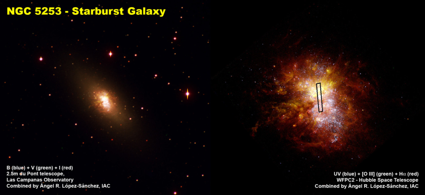
Figure 1: (Left) False color image in filters $B$ (blue), $V$ (green) and $I$ (red) of the starburst galaxy NGC 5253 observed by the 2.5m du Pont telescope, Las Campanas Observatory. (Right) False color image obtained by combining $HST$ H$\alpha$ (red), [O III] (green) and UV (blue) images. The position of our $VLT$ slit is indicated in it. North is up and east at left. The $HST$ image has been included at the center of the 2.5m du Pont telescope image for comparison.

NGC 5253 is also especially interesting because it is the best candidate for localized chemical enrichment in a GEHR. Welch (1970), Walsh & Roy (1987, 1989), and Kobulnicky et al. (1997) reported the presence of a strong nitrogen overabundance in a particular zone of the starbursting nucleus of the galaxy. Campbell et al. (1986) also found a helium enhancement in that zone, but this has not been confirmed in later works. Another peculiarity of the galaxy is that the majority of the gas seems to rotate about the optical major axis of the galaxy (Kobulnicky & Skillman, 1995) but this behaviour is not clear and could be combined with some kind of outflow (Koribalski 2006, priv. communication). However, CO observations by Turner, Beck, & Hurt (1997) and Meier, Turner & Beck (2002) suggest that molecular clouds are infalling into NGC 5253. These two observational facts indicate that the dynamical situation of this galaxy is far from clear. Other authors as van den Bergh (1980) and Cardwell & Phillips (1989) have suggested that the nuclear starburst was triggered as a result of a past interaction (around 1 Gyr ago) with the neighboring galaxy M83. Both galaxies lie at a radial distance of only 500 kpc and the projected separation is 130 kpc (Thim et al., 2003).

Concerning the kinematics of the ionized gas of NGC 5253, it has to be highlighted the presence of two large superbubbles related to the central region of the galaxy, with diameters of the order of 1 arcmin ($\sim$1 kpc), and expansion velocities of 35 km s^-1 (Marlowe et al., 1995). These superbubbles coincide with extended X-ray emission as demonstrated by Chandra and XMM-Newton data analyzed by Summers et al. (2004). The structure and morphology of the ionized gas in NGC 5253 were deeply analyzed by Calzetti et al. (2004) using imagery from Hubble Space Telescope (HST), detecting faint arches and filaments in both H$\alpha$ and [S II] at $\geq$1 kpc from the main ionizing cluster (see Figure 1, right panel) that are partially excited by shocks.

NGC 5253 has been considered as one of the youngest starbursts in the local universe (van den Bergh, 1980; Moorwood & Glass, 1982; Rieke et al., 1988). Campbell, Terlevich, & Melnick (1986) and Walsh & Roy (1987) reported a broad emission feature, indicating the presence of Wolf-Rayet (WR) stars in this galaxy. Several authors (Schaerer et al., 1997; Kobulnicky et al., 1997) have confirmed the presence of late-type WN and early-type WC stars. This fact, and the almost entirely thermal radio spectrum with very little synchrotron emission from supernova remants (Beck et al., 1996), imply the extreme youth of the starburst. Indeed, there is evidence in the literature that multiple starbursts in succession have occurred in the center of this galaxy, leaving behind an evolved, but still young-ish stellar population (Strickland & Stevens, 2000; Tremonti et al., 2001).

2 Observations and data reduction

The observations were made on 2003 March 30 with the Ultraviolet Visual Echelle Spectrograph, UVES (D’Odorico et al., 2000), at the Very Large Telescope, VLT, Kueyen unit in Cerro Paranal Observatory (Chile). The standard settings in both the red and blue arms of the spectrograph, covering the region from 3100 to 10400 Å, were used. The wavelength intervals 5783–5830 Å and 8540–8650 Å were not observed due to a gap between the two CCDs used in the red arm. There are also five small intervals that were not observed, 9608–9612 Å, 9761–9767 Å, 9918–9927 Å, 10080–10093 Å and 10249–10264 Å, because the five redmost orders did not fit completely within the CCD. The whole spectrum was taken in two different blocks of observations. The first block covers 3800-5000 Å with the blue arm and 6700–10400 Å with the red arm and was taken in three consecutive 1000s exposures. The second block, covering 3100–3900 Å and 4750–6800 Å, was taken in two consecutive 360s exposures. None of the emission lines was saturated in the exposures. The journal of the observations can be found in Table 1.

Table 1: Journal of observations.

$\Delta\lambda$	Exp. time	Spectral res.a	Spatial res.
(Å)	(s)	(Å pix-1)	($\arcsec$ pix-1)
3100–3900	2 x 360	0.019	0.25
3800–5000	3 x 1000	0.022	0.25
4750–6800	2 x 360	0.024	0.18
6700–10400	3 x 1000	0.033	0.17

^a At the center of each wavelength range.

The atmospheric dispersion corrector (ADC) was used to keep the same observed region within the slit regardless of the air mass value. This is especially important for this work because we extracted, analyzed and compared different small areas along the slit. The slit width was set to 1.5$\arcsec$ and the slit length was set to 10$\arcsec$ in the blue arm and to 12$\arcsec$ in the red arm. The slit width was chosen to maximize the S/N ratio of the emission lines, to separate most of the relevant faint lines, and to obtain a good spectral resolution for analyzing the velocity structure of the ionized gas. The effective resolution at a given wavelength is approximately $\Delta\lambda\sim\lambda/17600$. The seeing was excellent during the observations, $\sim$0.5 $\arcsec$.

In Figure 2 we show our slit position over the Figure 1 of Kobulnicky et al. (1997). The slit position was located along the north-south direction (P.A. = 0^∘), which was chosen in order to observe the most interesting regions inside the starburst. These zones were previously analyzed by Walsh & Roy (1989) and Kobulnicky et al. (1997). From north to south, these regions were designated HII-2, HII-1, UV1, and UV2 (A, B, C, and D, respectively), as it is shown in Figure 2. We have extracted 1-D spectra of the regions, with a size of 1.5$\arcsec\times 1.5\arcsec$.

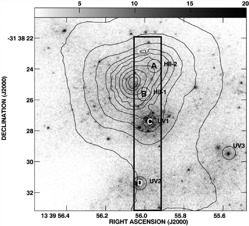
Figure 2: Our VLT slit position over Figure 1 of Kobulnicky et al. (1997), that shows the H$\alpha$ contours over the 2200 Å continuum image (gray scale). The four analyzed knots inside NGC 5253 are indicated and labeled.

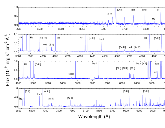
Figure 3: VLT UVES spectra of region B (HII-1). Some of the brightest emission lines are labeled. Telluric lines have not been removed and are specially evident in the 6600–9000 Å range. Note the gaps in the intervals 5783–5830 Å and 8540–8650 Å.

The spectra were reduced using the IRAF echelle reduction package, following the standard procedure of bias subtraction, flatfielding, wavelength calibration, aperture extraction and flux calibration. The standard stars EG 247, HD 49798, and C-32d9927 were observed for flux calibration. As an example, we show the wavelength- and flux-calibrated spectra of region B (HII-1) in Figure 3.

3 Line intensities
and reddening correction

Line intensities and equivalent widths were measured integrating all the flux in the line between two given limits and over a local continuum estimated by eye. In the cases of line blending, a multiple Gaussian profile fit procedure was applied to obtain the line flux of each individual line. The measurements were performed with the SPLOT routine of the IRAF package.

In Table 2 we have compiled all the emission lines detected in the four analyzed regions. Knot B (HII-1) is the zone where more lines have been identified: 169. Therefore, NGC 5253 is nowadays the dwarf starburst galaxy where more optical emission lines have been reported. We identify 156 lines in A (HII-2), 161 in C (UV1), and 86 in D (UV2). Besides the H I Paschen lines included in Table 2, some other lines were also detected, but they are blended with telluric spectral features, making it impossible to obtain a good determination of their intensity. The identification and adopted laboratory wavelength of the lines, as well as their errors, were obtained following García-Rojas et al. (2004); Esteban et al. (2004). Colons indicate errors of the order or greater than 40%.

Table 2: Dereddened line intensity ratios with respect to I(H$\beta$)=100.

$\lambda_{0}$ (Å)	Ion	Mult.	$f(\lambda)$	(A) HII-2	(B) HII-1	(C) UV-1	(D) UV-2
3187.84	He I	3F	0.308	4.01 $\pm$ 0.33	2.89 $\pm$ 0.28	3.82 $\pm$ 0.26	$\cdots$
3447.49	He I	7	0.295	$\cdots$	0.309:	$\cdots$	$\cdots$
3450.39	[Fe II]	27F	0.295	$\cdots$	0.063:	$\cdots$	$\cdots$
3530.50	He I	36	0.286	$\cdots$	0.152:	$\cdots$	$\cdots$
3554.42	He I	34	0.283	0.249:	0.158:	0.44 $\pm$ 0.11	$\cdots$
3587.28	He I	32	0.278	0.322:	0.191:	$\cdots$	$\cdots$
3613.64	He I	6	0.275	0.335:	0.356:	0.34 $\pm$ 0.10	$\cdots$
3634.25	He I	28	0.272	0.313:	0.411:	0.28 $\pm$ 0.10	$\cdots$
3651.97	He I	27	0.269	$\cdots$	0.093:	$\cdots$	$\cdots$
3664.68	H I	H28	0.267	$\cdots$	$\cdots$	0.24 $\pm$ 0.09	$\cdots$
3666.10	H I	H27	0.267	0.159:	0.124:	0.35 $\pm$ 0.10	$\cdots$
3667.28	H I	H26	0.266	0.130:	0.144:	0.276 $\pm$ 0.097	$\cdots$
3669.47	H I	H25	0.266	0.172:	0.183:	0.271 $\pm$ 0.097	$\cdots$
3671.48	H I	H24	0.266	0.166:	0.205:	0.256 $\pm$ 0.095	$\cdots$
3673.76	H I	H23	0.265	0.187:	0.255:	0.51 $\pm$ 0.12	$\cdots$
3676.37	H I	H22	0.265	0.284:	0.316:	0.51 $\pm$ 0.12	$\cdots$
3679.36	H I	H21	0.265	0.374:	0.229:	0.57 $\pm$ 0.12	$\cdots$
3682.81	H I	H20	0.264	0.365:	0.389:	0.68 $\pm$ 0.13	$\cdots$
3686.83	H I	H19	0.263	0.68 $\pm$ 0.20	0.56 $\pm$ 0.18	0.71 $\pm$ 0.13	$\cdots$
3691.56	H I	H18	0.263	0.91 $\pm$ 0.22	0.76 $\pm$ 0.19	0.97 $\pm$ 0.15	0.570:
3697.15	H I	H17	0.262	1.18 $\pm$ 0.23	1.01 $\pm$ 0.21	1.21 $\pm$ 0.16	1.021:
3703.86	H I	H16	0.260	1.30 $\pm$ 0.23	1.26 $\pm$ 0.22	1.24 $\pm$ 0.16	0.736:
3705.04	He I	25	0.260	0.58 $\pm$ 0.19	0.414:	0.49 $\pm$ 0.12	$\cdots$
3711.97	H I	H15	0.259	1.40 $\pm$ 0.24	1.27 $\pm$0.22	1.41 $\pm$ 0.17	1.324:
3721.83	[S III]	2F	0.257	2.95 $\pm$ 0.29	3.12 $\pm$ 0.28	3.24 $\pm$ 0.24	2.96 $\pm$ 0.69
3726.03	[O II]	1F	0.257	65.3 $\pm$ 2.3	62.9 $\pm$ 2.2	80.3 $\pm$ 2.9	145.4 $\pm$ 5.3
3728.82	[O II]	1F	0.256	71.9 $\pm$ 2.6	71.9 $\pm$ 2.6	102.2 $\pm$ 3.6	208.0 $\pm$ 7.2
3734.17	H I	H13	0.255	2.62 $\pm$ 0.28	2.16 $\pm$ 0.25	2.31 $\pm$ 0.20	2.60 $\pm$ 0.67
3750.15	H I	H12	0.253	3.14 $\pm$ 0.30	2.89 $\pm$ 0.27	2.80 $\pm$ 0.22	2.78 $\pm$ 0.68
3770.63	H I	H11	0.249	3.96 $\pm$ 0.32	3.62 $\pm$ 0.29	3.90 $\pm$ 0.26	4.59 $\pm$ 0.80
3797.90	H I	H10	0.244	5.32 $\pm$ 0.36	5.08 $\pm$ 0.33	5.13 $\pm$ 0.30	5.33 $\pm$ 0.84
3819.61	He I	22	0.240	1.10 $\pm$ 0.22	0.93 $\pm$ 0.20	0.94 $\pm$ 0.14	$\cdots$
3835.39	H I	H9	0.237	7.39 $\pm$ 0.28	7.37 $\pm$ 0.27	7.44 $\pm$ 0.28	7.27 $\pm$ 0.48
3856.02	Si II	1	0.233	0.079 $\pm$ 0.029	0.204 $\pm$ 0.031	0.086 $\pm$ 0.031	$\cdots$
3862.59	Si II	1	0.232	0.073 $\pm$ 0.029	0.084 $\pm$ 0.022	0.109 $\pm$ 0.034	0.52 $\pm$ 0.17
3868.75	[Ne III]	1F	0.230	48.8 $\pm$ 1.7	47.9 $\pm$ 1.6	34.1 $\pm$ 1.2	24.5 $\pm$ 1.0
3871.82	He I	60	0.230	$\cdots$	0.092 $\pm$ 0.023	0.038:	$\cdots$
3889.05	H I	H8	0.226	19.19 $\pm$ 0.67	17.91 $\pm$ 0.63	18.15 $\pm$ 0.64	18.67 $\pm$ 0.86
3926.53	He I	58	0.219	$\cdots$	0.070 $\pm$ 0.021	0.135 $\pm$ 0.036	$\cdots$
3964.73	He I	5	0.211	0.714 $\pm$ 0.063	0.680 $\pm$ 0.052	0.637 $\pm$0.063	0.336:
3967.46	[Ne III]	1F	0.210	13.81 $\pm$ 0.48	14.40 $\pm$ 0.50	9.51 $\pm$ 0.35	6.24 $\pm$ 0.46
3970.07	H I	H7	0.210	15.98 $\pm$ 0.55	16.03 $\pm$ 0.55	16.10 $\pm$ 0.56	15.83 $\pm$ 0.75
4009.22	He I	55	0.202	0.134 $\pm$ 0.034	0.232 $\pm$ 0.032	0.130 $\pm$ 0.035	$\cdots$
4026.21	He I	18	0.198	1.93 $\pm$ 0.10	1.815 $\pm$ 0.090	1.84 $\pm$ 0.10	1.51 $\pm$ 0.25
4068.60	[S II]	1F	0.189	2.37 $\pm$ 0.12	1.602 $\pm$ 0.082	1.484 $\pm$ 0.091	3.46 $\pm$ 0.35
4069.62	O II	10	0.189	$\cdots$	$\cdots$	0.054:	$\cdots$
4072.15	O II	10	0.188	$\cdots$	$\cdots$	0.020:	$\cdots$
4076.35	[S II]	1F	0.187	0.757 $\pm$ 0.064	0.490 $\pm$ 0.044	0.471 $\pm$ 0.055	1.17 $\pm$ 0.23
4097.26	O II	20-48	0.183	0.031:	$\cdots$	$\cdots$	$\cdots$
4101.74	H I	H6	0.182	26.00 $\pm$ 0.86	26.20 $\pm$ 0.86	26.05 $\pm$ 0.86	25.9 $\pm$ 1.0
4120.82	He I	16	0.177	0.152 $\pm$ 0.036	0.188 $\pm$ 0.030	0.094 $\pm$ 0.031	$\cdots$
4143.76	He I	53	0.172	0.212 $\pm$ 0.040	0.209 $\pm$ 0.031	0.199 $\pm$ 0.040	$\cdots$
4168.97	He I	52	0.167	$\cdots$	0.034:	0.039:	$\cdots$
4243.97	[Fe II]	21F	0.149	0.068 $\pm$ 0.027	0.069 $\pm$ 0.020	0.037:	0.124:
4267.15	C II	6	0.144	0.063 $\pm$ 0.026	0.074:	0.062 $\pm$ 0.026	$\cdots$
4276.83	[Fe II]	21F	0.142	0.023:	0.029:	0.019:	$\cdots$
4287.40	[Fe II]	7F	0.139	0.143 $\pm$ 0.034	0.108 $\pm$ 0.023	0.184 $\pm$ 0.039	0.40 $\pm$0.15
4303.61	O II	66	0.135	$\cdots$	$\cdots$	0.025:	$\cdots$
4340.47	H I	H$\gamma$	0.127	47.0 $\pm$ 1.5	46.8 $\pm$ 1.5	46.9 $\pm$ 1.5	46.9 $\pm$ 1.7
4359.34	[Fe II]	7F	0.122	0.067:	0.103 $\pm$ 0.023	0.099 $\pm$ 0.031	0.279:
4363.21	[O III]	2F	0.121	6.46 $\pm$ 0.23	6.70 $\pm$ 0.23	3.95 $\pm$ 0.16	2.61 $\pm$ 0.31
4368.25	O I	5	0.120	0.019:	0.068 $\pm$ 0.019	0.037:	$\cdots$
4387.93	He I	51	0.115	0.419 $\pm$ 0.049	0.474 $\pm$ 0.042	0.403 $\pm$ 0.050	0.322:
4413.78	[Fe II]	7F	0.109	$\cdots$	0.095 $\pm$ 0.022	0.073 $\pm$ 0.028	$\cdots$
4416.27	[Fe II]	6F	0.109	0.052:	0.045 $\pm$ 0.017	0.043:	$\cdots$
4437.55	He I	50	0.104	0.052:	0.044 $\pm$ 0.016	0.046:	$\cdots$
4452.11	[Fe II]	7F	0.100	0.049:	4.20 $\pm$ 0.16	0.032:	$\cdots$
4471.48	He I	14	0.095	4.11 $\pm$ 0.16	4.09 $\pm$ 0.15	3.79 $\pm$ 0.15	3.36 $\pm$ 0.34
4562.60	Mg I]	1	0.073	0.152 $\pm$ 0.034	0.108$\pm$ 0.022	0.129 $\pm$ 0.033	0.49 $\pm$ 0.16
4571.20	Mg I]	1	0.071	0.139 $\pm$ 0.033	0.102$\pm$ 0.022	0.115 $\pm$ 0.032	0.290:
4638.86	O II	1	0.055	0.040:	$\cdots$	0.049:	$\cdots$
4641.81	O II	1	0.054	0.066:	$\cdots$	0.060 $\pm$ 0.019	$\cdots$
4649.13	O II	1	0.052	0.063 $\pm$ 0.020	0.063 $\pm$ 0.021	0.062 $\pm$ 0.019	$\cdots$
4650.84	O II	1	0.052	0.034:	0.036:	0.042:	$\cdots$
4658.10	[Fe III]	3F	0.050	1.185 $\pm$ 0.074	1.134 $\pm$ 0.062	0.815$\pm$ 0.065	2.11 $\pm$ 0.28
4661.63	O II	1	0.049	0.027:	0.026:	0.061:	$\cdots$
4701.53	[Fe III]	3F	0.039	0.291 $\pm$ 0.042	0.339 $\pm$ 0.035	0.195 $\pm$ 0.038	0.340:
4711.37	[Ar IV]	1F	0.037	0.681 $\pm$ 0.058	0.890 $\pm$ 0.054	0.170 $\pm$ 0.036	$\cdots$
4713.14	He I	12	0.037	0.578 $\pm$ 0.054	0.587 $\pm$ 0.044	0.396 $\pm$ 0.049	$\cdots$
4733.93	[Fe III]	3F	0.031	0.090 $\pm$ 0.029	0.093 $\pm$ 0.021	0.048:	$\cdots$
4740.16	[Ar IV]	1F	0.030	0.723 $\pm$ 0.059	0.918 $\pm$ 0.055	0.135 $\pm$ 0.033	$\cdots$
4754.83	[Fe III]	3F	0.026	0.176 $\pm$ 0.035	0.157 $\pm$ 0.025	0.102 $\pm$ 0.030	0.240:
4769.60	[Fe III]	3F	0.023	0.131 $\pm$ 0.032	0.072 $\pm$ 0.019	0.058:	$\cdots$
4814.55	[Fe II]	20F	0.012	0.055:	0.044 $\pm$ 0.016	0.039:	$\cdots$
4861.33	H I	H$\beta$	0.000	100.0 $\pm$ 3.0	100.0 $\pm$ 3.0	100.0 $\pm$ 3.0	100.0 $\pm$ 3.2
4881.00	[Fe III]	2F	-0.005	0.345 $\pm$ 0.044	0.291 $\pm$ 0.032	0.170 $\pm$ 0.036	0.340:
4889.70	[Fe II]	3F	-0.007	0.028:	$\cdots$	$\cdots$	$\cdots$
4921.93	He I	48	-0.015	1.047 $\pm$ 0.068	1.016 $\pm$ 0.057	0.980 $\pm$ 0.069	0.82 $\pm$ 0.19
4931.32	[O III]	1F	-0.017	0.083 $\pm$ 0.027	0.056 $\pm$ 0.017	0.030:	$\cdots$
4958.91	[O III]	1F	-0.024	204.0 $\pm$ 6.1	206.2 $\pm$ 6.2	160.9 $\pm$ 4.8	104.3 $\pm$ 3.3
4985.90	[Fe III]	2F	-0.031	0.436 $\pm$ 0.061	0.459 $\pm$ 0.055	0.503 $\pm$ 0.051	1.85 $\pm$ 0.29
5006.84	[O III]	1F	-0.036	579 $\pm$ 17	597 $\pm$ 18	460 $\pm$ 13	300.2 $\pm$ 9.3
5015.68	He I	4F	-0.038	1.95 $\pm$ 0.12	2.18 $\pm$ 0.12	1.98 $\pm$ 0.11	1.76 $\pm$ 0.29
5041.03	Si II	5	-0.044	0.144 $\pm$ 0.039	0.205 $\pm$ 0.039	0.124 $\pm$ 0.026	0.53 $\pm$ 0.18
5047.74	He I	47	-0.046	0.277 $\pm$ 0.051	0.327 $\pm$ 0.048	0.311 $\pm$ 0.040	2.24 $\pm$ 0.32
5055.98	Si II	5	-0.048	0.346 $\pm$ 0.055	0.223 $\pm$ 0.040	0.300 $\pm$ 0.039	$\cdots$
5158.81	[Fe II]	19F	-0.073	$\cdots$	0.118 $\pm$ 0.031	0.181 $\pm$ 0.031	0.382:
5191.82	[Ar III]	3F	-0.081	0.158 $\pm$ 0.040	0.153 $\pm$ 0.034	0.089 $\pm$ 0.022	0.297:
5197.90	[N I]	1F	-0.082	0.318 $\pm$ 0.053	0.301 $\pm$ 0.045	0.220 $\pm$ 0.034	0.76 $\pm$ 0.20
5200.26	[N I]	1F	-0.083	0.251 $\pm$ 0.048	0.237 $\pm$ 0.041	0.147 $\pm$ 0.028	$\cdots$
5261.61	[Fe II]	19F	-0.098	0.074:	0.042:	0.061 $\pm$ 0.019	$\cdots$
5270.40	[Fe III]	1F	-0.100	0.466 $\pm$ 0.061	0.445 $\pm$ 0.053	0.324 $\pm$ 0.040	0.77 $\pm$ 0.21
5517.71	[Cl III]	1F	-0.154	0.375 $\pm$ 0.055	0.320 $\pm$ 0.045	0.362 $\pm$ 0.042	0.254:
5537.88	[Cl III]	1F	-0.158	0.289 $\pm$ 0.050	0.251 $\pm$ 0.040	0.271 $\pm$ 0.037	0.105:
5754.64	[N II]	3F	-0.194	0.500 $\pm$ 0.062	0.439 $\pm$ 0.050	0.177 $\pm$ 0.030	0.316:
5875.64	He I	11	-0.215	11.50 $\pm$ 0.43	12.34 $\pm$0.45	11.14 $\pm$ 0.42	10.74 $\pm$ 0.65
5957.56	Si II	4	-0.228	0.160 $\pm$ 0.039	$\cdots$	$\cdots$	$\cdots$
5978.93	Si II	4	-0.231	$\cdots$	0.035:	0.066 $\pm$ 0.019	$\cdots$
6300.30	[O I]	1F	-0.282	2.32 $\pm$ 0.13	2.15 $\pm$ 0.12	2.35 $\pm$ 0.12	6.05 $\pm$ 0.48
6312.10	[S III]	3F	-0.283	2.51 $\pm$ 0.14	2.43 $\pm$ 0.13	1.705 $\pm$ 0.099	1.53 $\pm$ 0.26
6347.11	Si II	2	-0.289	0.119 $\pm$ 0.034	0.076 $\pm$ 0.023	0.108 $\pm$ 0.023	$\cdots$
6363.78	[O I]	1F	-0.291	0.730 $\pm$ 0.072	0.677 $\pm$ 0.060	0.739 $\pm$ 0.060	1.90 $\pm$ 0.29
6371.36	Si II	2	-0.292	0.069 $\pm$ 0.027	0.130 $\pm$ 0.029	0.116 $\pm$ 0.024	0.137:
6548.03	[N II]	1F	-0.318	9.23 $\pm$ 0.39	8.21 $\pm$ 0.34	3.89 $\pm$ 0.18	7.63 $\pm$ 0.54
6562.82	H I	H$\alpha$	-0.320	282 $\pm$ 10	284 $\pm$ 10	288 $\pm$ 10	285.1 $\pm$ 9.8
6578.05	C II	2	-0.322	$\cdots$	$\cdots$	0.071 $\pm$ 0.019	$\cdots$
6583.41	[N II]	1F	-0.323	29.2 $\pm$ 1.1	24.61 $\pm$ 0.95	11.83 $\pm$ 0.48	22.5 $\pm$ 1.1
6678.15	He I	46	-0.336	3.38 $\pm$ 0.17	3.32 $\pm$ 0.16	3.00 $\pm$ 0.15	2.83 $\pm$ 0.34
6716.47	[S II]	2F	-0.342	13.37 $\pm$ 0.55	11.52 $\pm$ 0.47	13.90 $\pm$ 0.57	36.0 $\pm$ 1.5
6730.85	[S II]	2F	-0.344	12.44 $\pm$ 0.51	11.03 $\pm$ 0.45	12.17 $\pm$ 0.50	29.0 $\pm$ 1.3
7002.23	O I	21	-0.379	0.071:	0.087 $\pm$ 0.022	0.085 $\pm$ 0.020	0.244:
7065.28	He I	1/10	-0.387	4.36 $\pm$ 0.20	5.35 $\pm$ 0.23	3.04 $\pm$ 0.14	2.19 $\pm$ 0.23
7135.78	[Ar III]	1F	-0.396	13.51 $\pm$ 0.56	13.07 $\pm$ 0.54	10.40 $\pm$ 0.44	8.89 $\pm$ 0.45
7155.14	[Fe II]	14F	-0.399	0.047:	0.053 $\pm$ 0.019	0.048 $\pm$ 0.016	0.094:
7160.13	He I	1/10	-0.399	$\cdots$	0.015:	$\cdots$	$\cdots$
7281.35	He I	45	-0.414	0.579 $\pm$ 0.068	$\cdots$	0.451 $\pm$ 0.040	$\cdots$
7318.39	[O II]	2F	-0.418	2.73 $\pm$ 0.15	2.74 $\pm$ 0.13	2.78 $\pm$ 0.13	4.86 $\pm$ 0.32
7329.66	[O II]	2F	-0.420	2.09 $\pm$ 0.12	2.10 $\pm$ 0.10	2.23 $\pm$ 0.11	3.56 $\pm$ 0.28
7377.83	[Ni II]	2F	-0.425	0.074:	0.052 $\pm$ 0.019	0.083 $\pm$ 0.020	0.312:
7411.61	[Ni II]	2F	-0.429	0.019:	0.011:	0.016:	$\cdots$
7423.64	N I	3	-0.431	0.011:	0.010:	0.007:	$\cdots$
7442.30	N I	3	-0.433	0.028:	0.032:	0.035:	0.098:
7452.50	[Fe II]	14F	-0.434	0.024:	0.018:	0.017:	$\cdots$
7468.31	N I	3	-0.436	0.055:	0.061 $\pm$ 0.020	0.071 $\pm$ 0.019	0.159:
7499.85	He I	1/8	-0.439	0.029:	0.025:	0.360 $\pm$ 0.036	$\cdots$
7530.60	C II	16.08	-0.443	0.049:	0.051 $\pm$ 0.018	0.023:	$\cdots$
7751.10	[Ar III]	2F	-0.467	3.48 $\pm$ 0.18	3.15 $\pm$ 0.15	2.64 $\pm$ 0.13	2.17 $\pm$ 0.23
8000.08	[Cr III]	1F	-0.492	0.037:	0.047 $\pm$ 0.017	0.037:	$\cdots$
8045.63	[Cl IV]	1F	-0.497	0.109 $\pm$ 0.042	0.141 $\pm$ 0.025	0.032:	$\cdots$
8084.00	He I	4/18	-0.500	0.028:	$\cdots$	$\cdots$	$\cdots$
8125.31	Ca I]	::	-0.504	0.012:	$\cdots$	$\cdots$	$\cdots$
8210.72	N I	2	-0.512	0.014:	0.024:	$\cdots$	$\cdots$
8216.34	N I	2	-0.513	0.036:	0.026:	$\cdots$	$\cdots$
8223.14	N I	2	-0.514	0.046:	0.041 $\pm$ 0.016	$\cdots$	$\cdots$
8271.93	H I	P33	-0.518	$\cdots$	$\cdots$	0.045 $\pm$ 0.015	$\cdots$
8276.31	H I	P32	-0.518	$\cdots$	$\cdots$	0.046 $\pm$ 0.016	$\cdots$
8281.12	H I	P31	-0.519	$\cdots$	$\cdots$	0.059 $\pm$ 0.017	$\cdots$
8286.43	H I	P30	-0.519	$\cdots$	$\cdots$	0.091 $\pm$ 0.020	$\cdots$
8298.83	H I	P28	-0.521	$\cdots$	0.069 $\pm$ 0.018	0.084 $\pm$ 0.019	$\cdots$
8306.11	H I	P27	-0.521	$\cdots$	0.046 $\pm$ 0.015	0.066 $\pm$ 0.018	$\cdots$
8314.26	H I	P26	-0.522	0.089:	0.113 $\pm$ 0.022	0.095 $\pm$ 0.020	$\cdots$
8323.42	H I	P25	-0.523	0.095:	0.104 $\pm$ 0.021	0.143 $\pm$ 0.024	$\cdots$
8333.78	H I	P24	-0.524	$\cdots$	0.692 $\pm$ 0.050	0.903 $\pm$ 0.061	$\cdots$
8345.55	H I	P23	-0.525	0.111 $\pm$ 0.042	0.105 $\pm$ 0.021	0.156 $\pm$ 0.025	$\cdots$
8359.00	H I	P22	-0.526	0.181 $\pm$ 0.047	0.180 $\pm$ 0.026	0.217 $\pm$ 0.028	$\cdots$
8361.67	He I	1/6	-0.526	0.073:	0.059 $\pm$ 0.018	0.060 $\pm$ 0.017	$\cdots$
8374.48	H I	P21	-0.527	0.190 $\pm$ 0.048	0.182 $\pm$ 0.026	0.214 $\pm$ 0.028	$\cdots$
8392.40	H I	P20	-0.529	0.260 $\pm$ 0.052	0.232 $\pm$ 0.029	0.264 $\pm$ 0.031	0.49 $\pm$ 0.14
8413.32	H I	P19	-0.531	0.274 $\pm$ 0.052	0.229 $\pm$ 0.029	0.290 $\pm$ 0.032	31.6 $\pm$ 1.3
8437.96	H I	P18	-0.533	0.319 $\pm$ 0.055	0.300 $\pm$ 0.032	0.320 $\pm$ 0.034	0.137:
8446.36	O I	4	-0.534	0.645 $\pm$ 0.069	0.676 $\pm$ 0.049	0.688 $\pm$ 0.051	0.76 $\pm$ 0.16
8467.25	H I	P17	-0.536	0.373 $\pm$ 0.057	0.375 $\pm$ 0.036	0.369 $\pm$ 0.036	0.35 $\pm$ 0.13
8486.27	He I	6/16	-0.537	0.019:	0.018:	$\cdots$	$\cdots$
8502.48	H I	P16	-0.539	0.446 $\pm$ 0.061	0.454 $\pm$ 0.039	0.463 $\pm$ 0.041	0.43 $\pm$ 0.14
8665.02	H I	P13	-0.553	0.796 $\pm$ 0.075	1.003 $\pm$ 0.064	0.827 $\pm$ 0.058	0.59 $\pm$ 0.15
8680.28	N I	1	-0.554	0.049:	0.043 $\pm$ 0.016	0.044 $\pm$ 0.015	$\cdots$
8703.25	N I	1	-0.556	$\cdots$	0.024:	0.016:	$\cdots$
8711.70	N I	1	-0.556	0.027:	0.059 $\pm$ 0.018	0.054 $\pm$ 0.016	$\cdots$
8718.83	N I	1	-0.557	$\cdots$	0.020:	$\cdots$	$\cdots$
8733.43	He I	6/12	-0.558	0.019:	0.024:	0.013:	$\cdots$
8750.47	H I	P12	-0.560	1.057 $\pm$ 0.086	0.829 $\pm$ 0.056	1.442 $\pm$ 0.087	1.02 $\pm$ 0.17
8845.38	He I	6/11	-0.567	0.010:	0.027:	0.020:	$\cdots$
8862.79	H I	P11	-0.569	1.37 $\pm$ 0.10	1.400 $\pm$ 0.082	1.430 $\pm$ 0.087	1.32 $\pm$ 0.19
9014.91	H I	P10	-0.581	1.70 $\pm$ 0.11	1.551 $\pm$ 0.090	2.22 $\pm$ 0.13	1.67 $\pm$ 0.21
9068.90	[S III]	1F	-0.585	25.0 $\pm$ 1.3	25.5 $\pm$ 1.3	21.6 $\pm$ 1.1	17.94 $\pm$ 0.82
9123.60	[Cl II]	1F	-0.589	0.039:	0.036:	$\cdots$	$\cdots$
9229.01	H I	P9	-0.596	2.54 $\pm$ 0.15	2.63 $\pm$ 0.14	2.64 $\pm$ 0.15	2.65 $\pm$ 0.25
9530.60	[S III]	1F	-0.618	71.0 $\pm$ 8.5	63.8 $\pm$ 7.0	51.3 $\pm$ 6.2	43.7 $\pm$ 5.2
9545.97	H I	P8	-0.619	2.95 $\pm$ 0.18	3.20 $\pm$ 0.18	4.67 $\pm$ 0.25	2.69 $\pm$ 0.25
10031.20	He I	7/7	-0.649	0.214 $\pm$ 0.047	$\cdots$	$\cdots$	$\cdots$
10049.37	H I	P7	-0.650	6.18 $\pm$ 0.35	6.65 $\pm$ 0.36	5.62 $\pm$ 0.31	11.73 $\pm$ 0.60

The observed line intensities must be corrected for interstellar reddening. This can be done using the reddening constant, $c(H\beta)$, obtained from the intensities of H I lines. However, the fluxes of H I lines are also affected by underlying stellar absorption. Consequently, we have performed an iterative procedure to derive both $c(H\beta)$ and the equivalent widths of the absorption in the hydrogen lines, $W_{abs}$, that we use to correct the observed line intensities. As we have both H I Balmer and Paschen lines, we perform this procedure separately for them, following the procedure explained in López-Sánchez, Esteban & García-Rojas (2006).

Table 3: H$\beta$ fluxes, reddening coefficients and equivalent widths.

	(A) HII-2	(B) HII-1	(C) UV-1	(D) UV-2
$F$(H$\beta$) ($\times 10^{14}$ erg s-1 cm-2) ………………	13.45 $\pm$ 0.43	13.52 $\pm$ 0.42	10.13 $\pm$ 0.33	2.56 $\pm$ 0.09
$W$(H$\alpha$) (Å) ………………	919	1009	470	169
$W$(H$\beta$) (Å) ………………	234	254	94	39
$W$(H$\gamma$) (Å) ………………	96	93	43	44
$W$(H$\delta$) (Å) ………………	49	45	18	23
$W$(H$\epsilon$) (Å) ………………	27	25	11	5
$W$(H9) (Å) ………………	12	10	4	2
$W_{abs}$ (H$\alpha$) (Å)	0.0 $\pm$ 0.2	0.0 $\pm$ 0.2	0.0 $\pm$ 0.2	0.7 $\pm$ 0.2
$W_{abs}$ (H$\delta$) (Å)	0.7 $\pm$ 0.2	1.2 $\pm$ 0.2	0.4 $\pm$ 0.2	0.8 $\pm$ 0.2
$W_{abs}$ (H$\gamma$) (Å)	2.2 $\pm$ 0.2	3.9 $\pm$ 0.2	1.1 $\pm$ 0.2	0.8 $\pm$ 0.2
$W_{abs}$ (H$\epsilon$) (Å)	1.2 $\pm$ 0.2	1.5 $\pm$ 0.2	0.7 $\pm$ 0.2	0.4 $\pm$ 0.3
$W_{abs}$ (H9) (Å)	0.4 $\pm$ 0.3	0.9 $\pm$ 0.3	0.2 $\pm$ 0.3	0.2 $\pm$ 0.3
$W_{abs}$ (Balmer) (Å)	1.3 $\pm$ 0.3	1.7 $\pm$ 0.3	0.8 $\pm$ 0.2	0.6 $\pm$ 0.3
$c$(H$\beta$) (Balmer)	0.22 $\pm$ 0.02	0.36 $\pm$ 0.03	0.23 $\pm$ 0.03	0.09 $\pm$ 0.02
$W_{abs}$ (Paschen) (Å)	0.0 $\pm$ 0.1	0.0 $\pm$ 0.1	0.0 $\pm$ 0.1	0.0 $\pm$ 0.1
$c$(H$\beta$) (Paschen)	0.24 $\pm$ 0.02	0.39 $\pm$ 0.02	0.27 $\pm$ 0.02	0.10 $\pm$ 0.02
$c$(H$\beta$) (adopted)	0.23 $\pm$ 0.02	0.38 $\pm$ 0.03	0.25 $\pm$ 0.03	0.10 $\pm$ 0.02

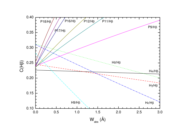
Figure 4: Reddening constant, $c(H\beta)$, as a function of the absorption equivalent width in the hydrogen lines. Each straight line represent the behaviour of the ratio of a given Balmer and Paschen line with respect to H$\beta$.

In Figure 4 we plot the reddening constant, $c(H\beta)$, versus the absorption equivalent widths in the hydrogen lines, $W_{abs}$, for the data of region A. It can be noted that absorption in the H I Paschen lines is practically negligible. This result is also found in the rest of analyzed regions. However, H I Balmer lines have considerably differences in their $W_{abs}$, although the $c(H\beta)$ derived from them is very similar to those derived from Paschen lines. We have assumed the average value between the $c(H\beta)$ derived from Balmer and Paschen lines as representative of the region. This value can be used to estimate the appropriate value of $W_{abs}$ for each Balmer line. The $c(H\beta)$ and $W_{abs}$ that provide the best match between the corrected and the theoretical Balmer and Paschen line ratios, as well as the finally adopted values of $c(H\beta)$ and $W_{abs}$ for the brightest Balmer lines are shown in Table 3.

4 Emission line profiles
and gas kinematics

Our observations confirm the presence of asymmetric wings in the line profiles at the center of NGC 5253, as were previously reported in echelle spectra by Martin & Kennicutt (1995) and Marlowe et al. (1995). The line-profiles of regions A and B show a broader intense component underlying a narrower one with velocity shifts of the order of lower than 10 km s^-1. This broad component is redshifted with respect to the narrow one in zone A, but appears slightly blueshifted in region B. Region C seems to show a rather faint broad component. Finally, the line profiles of region D seem to be composed by the combination of two similar narrow components with a velocity shift of $\sim$ 35 km s^-1. Consistent values of the velocity shift between components were found by Martin & Kennicutt (1995) and Marlowe et al. (1995).

The velocity separation between components reaches a maximum at zone D. The maximum width of the broad component occurs in regions A and B where the full width at half maximum (FWHM) reaches values of the order of 110 km s^-1. Martin & Kennicutt (1995) report consistent values of the FWHM of this component. The velocity shifts and FWHM ratio between broad and narrow component for other lines like [O II], [O III], [N II], and [S II] are qualitatively similar for a given zone. Similar complex emission-line profiles and FWHM of the broad components were found by Marlowe et al. (1995) and Méndez & Esteban (1997) for different samples of dwarf starburst galaxies.

The high signal-to-noise of our spectra has permitted to perform a spatially resolved analysis of the kinematics of the ionized gas observed in the center of NGC 5253. It was studied via the analysis of the centroids of the total line profiles of H$\alpha$, [O II] $\lambda\lambda$3726,3729, [N II] $\lambda$6583 and [S III] $\lambda$9069 along the slit position. We have extracted zones of 3 pixels wide that corresponds to 0.54$\arcsec$ in the sky for the H$\alpha$ and [N II] emission lines and 0.51$\arcsec$ for the [S III] line. The width of the extracted zones for the position of [O II] is 2 pixels, that corresponds to 0.50$\arcsec$. In Figure 5 we show the position-velocity (PV) diagrams obtained. All the velocities are referred to the velocity of the center of region B (HII-1).

Figure 5 indicates that the ionized gas at the center of NGC 5253 follows a sinusoidal pattern, indicating that its kinematics is not due to pure rotation. The behaviour of our PV diagram is in agreement (considering the shape and the velocity amplitudes) with that obtained by Martin & Kennicutt (1995) for their slit positions 2 and 3 in the central zones of the galaxy. The sinusoidal or wave-like pattern may be produced by distortions produced by the presence of dynamically decoupled gas systems (e.g. Schweizer 1982). This explanation would imply that a merging process is ongoing in the central zone of the galaxy. Another possibility is that the velocity pattern is produced by the outflow from the central starbursts. In fact, the wave-like forms produced by supershells are rather common in starbursting dwarf galaxies (Martin & Kennicutt, 1995; Marlowe et al., 1995; Pustilnik et al., 2004). We also find that the PV diagrams of the narrow and broad components are similar, it would imply that the outflows affect the dynamics of both components in a similar way. It is remarkable that the PV diagrams derived from emission lines of different ions are in excellent agreement except for the [N II] $\lambda$6583 line at regions A (HII-2) and B (HII-1). This fact could be related to a possible localized nitrogen pollution in those zones (we discuss this in §12).

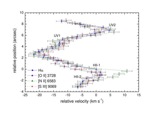
Figure 5: Position-velocity diagram for the slit position observed using H$\alpha$, [O II] $\lambda\lambda$3726,3729, [N II] $\lambda$6583 and [S III] $\lambda$9069 emission lines. The abscissa shows velocities with respect to the center of zone B.

Table 4: Physical Conditions of the Ionized Gas

Diagnostic	Lines	(A) HII-2	(B) HII-1	(C) UV-1	(D) UV-2
$n_{\rm e}$ (cm-3)	[O II] ($\lambda$3726)/($\lambda$3729)	660${}^{+130}_{-140}$	600${}^{+120}_{-130}$	420$\pm 100$	270 $\pm$ 80
	[S II] ($\lambda$6716)/($\lambda$6731)	460${}^{+160}_{-210}$	530${}^{+170}_{-220}$	330${}^{+130}_{-180}$	190${}^{+110}_{-150}$
	[N I] ($\lambda$5198)/($\lambda$5200)	670 ${}^{+550}_{<100}$	670${}^{+510}_{<100}$	1140::	$\cdots$
	[Cl III] ($\lambda$5518)/($\lambda$5538)	530:	640:	380:	$\cdots$
	[Fe III]	750 $\pm$ 250	650 $\pm$ 350	350 $\pm$ 300	300 $\pm$ 300
	[Ar IV] ($\lambda$4711)/($\lambda$4740)	5600${}^{+3400}_{-2600}$	5100${}^{+2200}_{-1900}$	1300${}^{+7200}_{-1300}$	$\cdots$
	Adopted valueb	580 $\pm$ 110	610 $\pm$ 100	370 $\pm$ 80	230 $\pm$ 70
$T_{\rm e}$ (K) High	[O III] ($\lambda$4959+$\lambda$5007)/($\lambda$4363)	11960${}^{+270}_{-300}$	12010${}^{+270}_{-300}$	10940${}^{+240}_{-270}$	10990${}^{+490}_{-620}$
	[S III] ($\lambda$9069+$\lambda$9532)/($\lambda$6312)a	12330${}^{+640}_{-800}$	11970${}^{+580}_{-720}$	10910${}^{+510}_{-630}$	11300${}^{+1000}_{-1600}$
	[Ar III] ($\lambda$7136+$\lambda$7751)/($\lambda$5192)	12000${}^{+1200}_{-2200}$	12100${}^{+1100}_{-1900}$	10600${}^{+940}_{-1600}$	$\cdots$
	Adopted value	12100 $\pm$ 260	12030 $\pm$ 260	10810 $\pm$ 230	11160 $\pm$ 510
$T_{\rm e}$ (K) Low	[O II] ($\lambda$3726+$\lambda$3729)/($\lambda$7320+$\lambda$7330)	11300${}^{+600}_{-740}$	11330${}^{+560}_{-680}$	10660${}^{+490}_{-590}$	10570${}^{+580}_{-740}$
	[S II] ($\lambda$6716+$\lambda$6731)/($\lambda$4069+$\lambda$4076)	10880${}^{+860}_{-1160}$	8680${}^{+550}_{-720}$	8180${}^{+530}_{-710}$	8380${}^{+760}_{-1130}$
	[N II] ($\lambda$6548+$\lambda$6583)/($\lambda$5755)	11040${}^{+700}_{-960}$	11170${}^{+680}_{-920}$	10410${}^{+780}_{-11600}$	10100${}^{+1500}_{-4200}$
	Adopted valuec	11170 $\pm$ 520	11250 $\pm$ 490	10530 $\pm$ 470	10350 $\pm$ 650
$T_{\rm e}$ (K)	He I	10270 $\pm$ 300	10200 $\pm$ 300	9000 $\pm$ 300	10600 $\pm$ 450

5 Physical conditions of the ionized gas

We have derived the electron temperature, $T_{e}$, and density, $n_{e}$, of the ionized gas using several emission line ratios. The values obtained for each region are compiled in Table 4. All determinations were computed with the IRAF task TEMDEN on the NEBULAR package (Shaw & Dufour, 1995), except for the density derived from [Fe III] emission lines (see below). We have changed the default atomic data of O⁺, S⁺, and S⁺⁺ included in the last version of NEBULAR (February 2004) by other datasets that we consider give better results. These changes are indicated in Table 4 of García-Rojas et al. (2004).

In order to derive $n_{e}$, we have used several emission line ratios between CELs (see Table 4) and the intensities of several [Fe III] lines. The [Fe III] density was computed from the intensity of the brightest lines of each region (those with errors less than 30% and not affected by line blending) and applying the computations of Rodríguez (2002). All the values of $n_{e}$ are consistent within the errors (see Table 4) except those obtained from the [Ar IV] lines, which are always higher and are expected to be representative of the inner zones of the nebulae. In the case of zones A and B that difference is almost one order of magnitude indicating a strong density stratification in the ionized gas.

Once $n_{e}$ was obtained we used it to derive $T_{e}$ using [O III], [S III], [Ar III], [O II], [S II], and [N II] line ratios, and we iterated until convergence. We have determined the characteristic temperature of the helium zone, $T_{e}$(He I), in the presence of temperature fluctuations (see §7) using the formulation of Peimbert, Peimbert, & Luridiana (2002). All determinations of $T_{e}$ are included in Table 4. It is important to remark that previous $T_{e}$ determinations in the literature were restricted to a single indicator: $T_{e}$(O III). The values of $T_{e}$(O III) determined by Kobulnicky et al. (1997) are consistent with those derived from our data.

We have assumed a two-zone approximation to describe the temperature structure of the nebulae. Therefore, we used the mean of $T_{e}$(O III), $T_{e}$(S III) and $T_{e}$(Ar III) as the representative temperature for high ionization potential ions whereas the mean of $T_{e}$(O II) and $T_{e}$(N II) was assumed for the low ionization potential ion temperatures. We do not include $T_{e}$(S II) in the average because its value is around 1500 K lower that the ones obtained from [O II] and [N II] ratios in three of the zones. This difference is also reported in the Galactic H II region S 311 by García-Rojas et al. (2005) and might be produced by the presence of a temperature stratification in the outer zones of the nebulae.

6 Ionic Abundances

The large collection of emission lines measured in the spectra has permitted the derivation of abundances for an unprecedented large number of ions in NGC 5253 from both recombination and collisionally excited lines.

6.1 He⁺ abundance

Table 5: He⁺/H⁺ ratios^a

Line	(A) HII-2	(B) HII-1	(C) UV-1	(D) UV-2
3819.61	830 $\pm$ 166	704 $\pm$ 152	707 $\pm$ 106	$\cdots$
3964.73	642 $\pm$ 88	603 $\pm$ 46	579 $\pm$ 57	$\cdots$
4026.21	821 $\pm$ 43	775 $\pm$ 38	772 $\pm$ 42	653 $\pm$ 108
4387.93	676 $\pm$ 79	769 $\pm$ 69	649 $\pm$ 81	$\cdots$
4471.09	876 $\pm$ 34	794 $\pm$ 29	736 $\pm$ 27	676 $\pm$ 68
4713.14	899 $\pm$ 84	826 $\pm$ 61	691 $\pm$ 84	$\cdots$
4921.93	775 $\pm$ 50	759 $\pm$ 43	722 $\pm$ 51	625 $\pm$ 145
5875.64	777 $\pm$ 29	840 $\pm$ 31	758 $\pm$ 29	786 $\pm$ 48
6678.15	836 $\pm$ 42	838 $\pm$ 41	735 $\pm$ 37	741 $\pm$ 90
7065.28	803 $\pm$ 37	786 $\pm$ 34	729 $\pm$ 34	732 $\pm$ 77
7281.35	775 $\pm$ 91	$\cdots$	632 $\pm$ 56	$\cdots$
Adoptedb	807 $\pm$ 16	791 $\pm$ 14	729 $\pm$ 13	737 $\pm$ 34
$\tau_{3889}$	9.61 $\pm$ 0.74	11.68 $\pm$ 0.70	7.33 $\pm$ 0.70	1.61 $\pm$ 0.92
$\chi^{2}$	18.19	19.54	12.67	3.35

We have measured a large number of He I lines in our spectra of NGC 5253, the maximum in region A where we detect 34 lines. This permits to determine the He⁺/H⁺ ratio with much better precision than in previous studies. We have followed the same method explained in García-Rojas et al. (2005), who applied the maximum likelihood method developed by Peimbert, Peimbert, & Ruiz (2000) to derive the He⁺/H⁺ ratio and some physical properties of the ionized gas. In Table 5 we include the He⁺/H⁺ ratios for each individual He I line and the final adopted average value for each region $<$He⁺/H⁺$>$. In that table, we also include the corresponding value of $\tau_{3889}$ obtained from the maximum likelihood method as well as the corresponding $\chi^{2}$ parameter, which indicates a reasonable goodness of the fit obtained by the method in the four regions.

6.2 Ionic abundances from CELs

Table 6: Ionic abundances from collisionally excited lines

12 + log(Xm/H+)	(A) HII-2		(B) HII-1		(C) UV-1		(D) UV-2
	$t^{2}$=0.00	$t^{2}$=0.072$\pm$0.027	$t^{2}$=0.00	$t^{2}$=0.050$\pm$0.035	$t^{2}$=0.00	$t^{2}$=0.061$\pm$0.024	$t^{2}$=0.00
N+	6.62 $\pm$ 0.04	6.81 $\pm$ 0.10	6.55 $\pm$ 0.04	6.67 $\pm$ 0.12	6.30 $\pm$ 0.05	6.48 $\pm$ 0.10	6.61 $\pm$ 0.06
O+	7.59 $\pm$ 0.06	7.80 $\pm$ 0.11	7.58 $\pm$ 0.05	7.72 $\pm$ 0.12	7.81 $\pm$ 0.06	8.01 $\pm$ 0.11	8.11 $\pm$ 0.08
O++	8.05 $\pm$ 0.03	8.34 ${}^{+0.15}_{-0.12}$	8.07 $\pm$ 0.03	8.26 ${}^{+0.16}_{-0.13}$	8.10 $\pm$ 0.03	8.39 $\pm$ 0.14	7.87 $\pm$ 0.05
Ne++	7.34 $\pm$ 0.05	7.65 ${}^{+0.16}_{-0.14}$	7.36 $\pm$ 0.05	7.56 ${}^{+0.18}_{-0.15}$	7.36 $\pm$ 0.05	7.67 ${}^{+0.17}_{-0.15}$	7.15 $\pm$ 0.09
S+	5.70 $\pm$ 0.05	5.89 $\pm$ 0.10	5.64 $\pm$ 0.05	5.76 ${}^{+0.12}_{-0.10}$	5.75 $\pm$ 0.05	5.93 $\pm$ 0.09	6.15 $\pm$ 0.07
S++	6.45 $\pm$ 0.05	6.77 $\pm$ 0.16	6.44 $\pm$ 0.05	6.64 ${}^{+0.18}_{-0.15}$	6.45 $\pm$ 0.05	6.76 ${}^{+0.17}_{-0.14}$	6.35 $\pm$ 0.07
Cl+	4.07:	4.24:	4.03:	4.14:	$\cdots$	$\cdots$	$\cdots$
Cl++	4.39 $\pm$ 0.08	4.67 ${}^{+0.16}_{-0.14}$	4.33 $\pm$ 0.06	4.51 ${}^{+0.17}_{-0.14}$	4.50 $\pm$ 0.07	4.77 ${}^{+0.16}_{-0.13}$	4.19 $\pm$ 0.25
Cl3+	3.73 $\pm$ 0.16	3.96 $\pm$ 0.19	3.85 $\pm$ 0.09	4.00 $\pm$ 0.15	3.30 $\pm$ 0.17	3.53 $\pm$ 0.20	$\cdots$
Ar++	5.93 $\pm$ 0.04	6.18 ${}^{+0.13}_{-0.11}$	5.90 $\pm$ 0.04	6.06 ${}^{+0.14}_{-0.12}$	5.92 $\pm$ 0.04	6.16 $\pm$ 0.13	5.81 $\pm$ 0.07
Ar3+	4.88 $\pm$ 0.06	5.18 $\pm$ 0.15	5.00 $\pm$ 0.05	5.19 ${}^{+0.17}_{-0.15}$	4.34 $\pm$ 0.11	4.63 ${}^{+0.18}_{-0.16}$	$\cdots$
Fe+	4.53:	4.71:	4.58:	4.70:	4.62:	4.79:	4.96:
Fe++	5.53 $\pm$ 0.08	5.83 $\pm$ 0.16	5.48 $\pm$ 0.08	5.67 ${}^{+0.18}_{-0.16}$	5.42 $\pm$ 0.11	5.71 ${}^{+0.18}_{-0.16}$	5.89 ${}^{+0.11}_{-0.13}$
log(N+/O+)	–0.97 $\pm$ 0.07	–0.99 $\pm$0.14	–1.02 $\pm$ 0.07	–1.05 $\pm$0.16	–1.51 $\pm$ 0.07	–1.53 $\pm$0.14	–1.51 $\pm$ 0.10

The IRAF package NEBULAR has been used to derive ionic abundances of O⁺, O⁺⁺, N⁺, S⁺, S⁺⁺, Ne⁺⁺, Ar⁺⁺, Ar⁺³, Cl⁺⁺, and Cl⁺³ for each region from the intensity of CELs. The electron densities and temperatures for the high and low ionization potential ions used are those corresponding to the aforementioned two-zone scheme. The finally adopted ionic abundances are listed in Table 6, they correspond to the mean of the abundances derived from all the observed individual lines of each ion and weighted by their relative intensities. Errors were estimated from the uncertainties in electron density and temperature and those associated to the line intensity ratio with respect to H$\beta$. Fe⁺⁺ abundances have been derived from 6 or 7 [Fe III] lines except in the case of zone D, where only three lines were used. The lines selected for the derivation of the Fe⁺⁺/H⁺ ratios are those not affected by line-blending and with line flux uncertainties less than 30%. We have used a 34 level model atom that includes the collision strengths calculated by Zhang (1996) and the transition probabilities given by Quinet (1996). Fe⁺⁺ abundances are also included in Table 6.

We have detected several [Fe II] lines in our spectra, but they are severely affected by fluorescence effects (Rodríguez, 1999; Verner et al., 2000). Unfortunately, the [Fe II] $\lambda$8617 line, which is almost insensitive to fluorescence effects, is not observed because it lies in one of our narrow observational gaps. However, we have measured [Fe II] $\lambda$7155, a line which does not seem to be affected by fluorescence effects (Rodríguez, 1996). We have derived Fe⁺ abundances from this line, assuming that $I$(7155)/$I$(8617) $\sim$ 1 (Rodríguez, 1996), and using the calculations of Bautista & Pradhan (1996). The results obtained imply low concentrations of Fe⁺ (see Table 6). Due to the faintness of the [Fe II] $\lambda$7155 line, and to the assumption adopted, the derived Fe⁺ abundances are only rough estimates and will not be used in the Fe abundance determination.

We have detected [Cl II] lines in two of the observed zones. However, the Cl⁺/H⁺ ratio cannot be derived from the NEBULAR routines because the atomic data of this ion is not included, instead we have used an old version of the five-level atom program of Shaw & Dufour (1995) that is described by De Robertis, Dufour, & Hunt (1987). This version uses the atomic data for Cl⁺ compiled by Mendoza (1983), which are rather uncertain (Shaw 2003, personal communication). Therefore the Cl⁺/H⁺ ratio given in Table 6 should be interpreted as a rough approximation to the true one.

6.3 Ionic abundances from RLs

Table 7: O⁺⁺ and C⁺⁺ abundances from recombination lines^a

	(A) HII-2		(B) HII-1		(C) UV 1
	LTE	NLTE	LTE	NLTE	LTE	NLTE
O II $\lambda$4638.86 ………………………	38:	20:	$\cdots$	$\cdots$	47:	24:
O II $\lambda$4641.81 ………………………	23:	27:	$\cdots$	$\cdots$	21 $\pm$ 7	25 $\pm$ 8
O II $\lambda$4649.13 ………………………	12 $\pm$ 4	25 $\pm$ 8	12 $\pm$ 4	25 $\pm$ 8	12 $\pm$ 4	29 $\pm$ 9
O II $\lambda$4650.84 ………………………	34:	16:	36:	17:	42:	18:
O II $\lambda$4661.63 ………………………	21:	12:	20:	12:	47:	26:
Sum value (all lines) ………..	20	22	17	20	24	25
O++/H+ adopted value	20 $\pm$ 8		18 $\pm$ 7		24 $\pm$ 10
12+log(O++/H+) (RLs)	8.30 $\pm$ 0.15		8.26 $\pm$ 0.15		8.38 $\pm$ 0.15
12+log(O++/H+) (CELs)	8.05 $\pm$ 0.03		8.07 $\pm$ 0.03		8.10 $\pm$ 0.03
C II $\lambda$4267.15 ………………………	6 $\pm$ 2		5:		6 $\pm$ 3
12+log(C++/H+) (RLs)	7.82${}^{+0.14}_{-0.22}$		7.75:		7.81${}^{+0.15}_{-0.23}$
12+log(C++/H+) (CELs)b	7.41${}^{+0.16}_{-0.18}$		7.43 $\pm$ 0.17		7.48 $\pm$ 0.23
log(C++/O++) (RLs)	$-$0.48${}^{+0.37}_{-0.41}$		$-0.51$:		$-$0.57${}^{+0.33}_{-0.36}$
log(C++/O++) (CELs)b	$-$0.62${}^{+0.19}_{-0.20}$		$-$0.64${}^{+0.16}_{-0.18}$		$-$0.59${}^{+0.25}_{-0.26}$

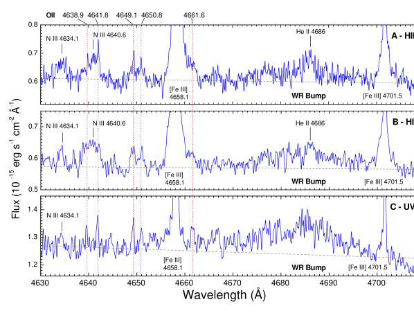
Figure 6: Sections of echelle spectra of zones A, B, and C of NGC 5253 showing the lines of multiplet 1 of O II and the WR bump. Note the broad N III $\lambda$4641 emission line blended with O II $\lambda\lambda$4639,4642 emission lines in regions A and B. That line is absent in region C. A broad N III $\lambda$4634 seems to be also present in region A.

One of the main goals of this work has been the measurement of RLs of heavy element ions in NGC 5253, the first dwarf starburst galaxy where these kinds of lines have been unambiguously detected. Three of the four zones observed show the presence of RLs of heavy element ions in their spectra. These lines are those belonging to multiplet 1 of O II (see Figure 6) and C II $\lambda$4267 (see Figure 7). All these lines are produced by pure recombination [see Esteban et al. (1998, 2004), and references therein] and their intensities depend weakly on electron temperature and density. We have computed the abundances assuming the adopted values of $n_{e}$ and $T_{e}$(High) given in Table 4 for each zone. The atomic data used and the methodology for the derivation of the abundances from RLs are the same as in García-Rojas et al. (2004). The lines of multiplet 1 of O II are not in LTE for densities $n_{e}<$10000 cm^-3 (Ruiz et al., 2003). We have used the prescriptions given by Peimbert, Peimbert, & Ruiz (2005) to calculate the appropriate corrections for the abundances obtained from individual O II lines. These corrected abundances show very good agreement with those obtained using the sum of the intensities of all the lines of the multiplet, which is not affected by non LTE effects. Table 7 shows the O⁺⁺/H⁺ and C⁺⁺/H⁺ ratios obtained from individual RLs as well as the correction for non LTE effects and the corresponding sum values for the O II lines. In that table we also compare with the same ratios obtained from CELs. In the case of the C⁺⁺/H⁺ ratio, we have compared our determinations based on RLs with those obtained by Kobulnicky et al. (1997) from UV CELs for exactly the same zones but with a slightly smaller aperture. Consistently with the result found for O⁺⁺/H⁺, the C⁺⁺/H⁺ ratios derived from RLs are systematically larger than those derived from CELs.

7 Abundance Discrepancy
and Temperature Fluctuations

Table 8: NGC 5253 $t^{2}$ parameter

Method	$t^{2}$
	(A) HII-2	(B) HII-1	(C) UV-1
O++ (R/C)	0.064 $\pm$ 0.035	0.050 $\pm$ 0.035	0.060 $\pm$ 0.030
C++ (R/C)	0.084 ${}^{+0.027}_{-0.049}$	0.073:	0.062 ${}^{+0.027}_{-0.052}$
Adopted	0.072 $\pm$ 0.027	0.050 $\pm$ 0.035	0.061 $\pm$ 0.024

As it can be seen in Table 7, the discrepancy between ionic abundances obtained from RLs and CELs are between 0.19 and 0.28 dex in the case of O⁺⁺/H⁺ and between 0.30 and 0.40 dex in the case of C⁺⁺/H⁺. Very similar values have been obtained for different Galactic and extragalactic H II regions. Torres-Peimbert et al. (1980) proposed that the abundance discrepancy could be related to the presence of spatial temperature fluctuations because of the different functional temperature dependence of RLs and CELs. Table 8 shows the different determinations of $t^{2}$ and our final adopted value. The two upper rows of the table show the $t^{2}$ parameters that make the O⁺⁺ and C⁺⁺ abundances obtained from RLs and CELs to coincide [denoted as O⁺⁺(C/R) and C⁺⁺(C/R) in the table]. We can see that these two $t^{2}$ values are consistent within the errors for all the zones. The final adopted value of $t^{2}$ is the weighted average of the individual determinations for each zone.

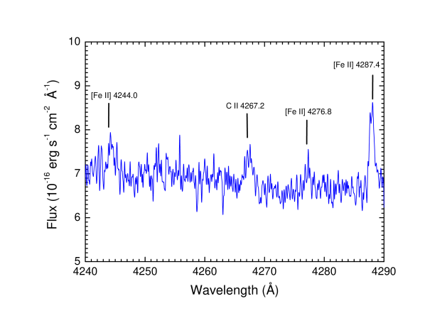
Figure 7: Section of echelle spectrum of region A of NGC 5253 showing the C II $\lambda$4267 line.

8 Total Abundances

Total abundances have been determined for He, C, N, O, Ne, S, Cl, Ar, and Fe and are shown in Table 9. The non-detection of the nebular He II $\lambda$4686 line in our deep spectra implies the absence of a significant amount of He⁺⁺ and O³⁺ in the ionized gas of NGC 5253. Then, the use of the relation O/H = O⁺/H⁺ + O⁺⁺/H⁺ is entirely justified. For the rest of the elements, we have to adopt a set of ionization correction factors (ICFs) to correct for the unseen ionization stages.

For carbon we have adopted the ICF derived from photoionization models by Garnett et al. (1999). This correction seems to be fairly appropriate considering the high ionization degree of the three brightest zones of NGC 5253 where the C II line has been detected.

In the case of neon we have applied the classical ICF proposed by Peimbert & Costero (1969), that assumes that the ionization structure of Ne is similar to that of O. This is a very good approximation for high ionization degree objects, where a small fraction of Ne⁺ is expected. Martín-Hernández, Schaerer, & Sauvage (2005), using $N$-band NIR spectroscopy, have estimated 12+log(Ne⁺/H⁺)=6.46, for a zone located between our regions A and B. Assuming this Ne⁺ abundance for A and B we obtain an ICF of $\sim$1.12, somewhat lower than the value of $\sim$1.36 that gives our adopted ICF scheme.

We have measured two ionization stages of S, S⁺ and S⁺⁺, in all regions, but a significant contribution of S³⁺ is expected. We have adopted the ICF given by Stasińska (1978), which is based on photoionization models of H II regions and is expressed as a function of the O⁺/O ratio.

We have measured lines of all possible ionization stages of chlorine in two of the zones (A and B). In any case, as it can be seen in Table 6, the dominant ionization stage is Cl⁺⁺ and the contribution of Cl⁺ to the total abundance is rather small, at least in the high ionization degree regions as A, B, and C. Hence, we have neglected any contribution of the singly ionized stage for the determination of the total abundance of chlorine in zone C. In the case of region D, its lower ionization recommends to take into account the Cl⁺ fraction, for that, we have adopted the relation by Peimbert & Torres-Peimbert (1977).

For argon we have determinations of the Ar⁺⁺ and Ar³⁺ abundances. We find that Ar⁺⁺ is almost one order of magnitude more abundant than Ar³⁺, indicating that most Ar is in the form of Ar⁺⁺. However, some contribution of Ar⁺ is expected. Martín-Hernández, Schaerer, & Sauvage (2005) have obtained an upper limit for Ar⁺/Ar⁺⁺ $<$ 0.35 for a zone located between our regions A and B. In our case, we have adopted the ICF of Izotov, Thuan, & Lipovetski (1994).

For Fe, we have measured lines of two stages of ionization of iron: Fe⁺ and Fe⁺⁺, but we expect an important contribution of Fe³⁺. Since the Fe⁺ contribution is small and uncertain, (see § 6.2) the total iron abundance have been obtained from the Fe⁺⁺/H⁺ ratio and the ICF obtained by Rodríguez & Rubin (2005).

Table 9: Total abundances and abundance ratios

12 + log(X/H)	(A) HII-2		(B) HII-1		(C) UV-1		(D) UV-2
	$t^{2}$=0.00	$t^{2}$=0.072$\pm$0.027	$t^{2}$=0.00	$t^{2}$=0.050$\pm$0.035	$t^{2}$=0.00	$t^{2}$=0.061$\pm$0.024	$t^{2}$=0.00
Hea	10.97 $\pm$ 0.02	10.95 $\pm$ 0.02	10.95 $\pm$ 0.01	10.94 $\pm$ 0.02	10.93 $\pm$ 0.02	10.91 $\pm$ 0.02	11.08 $\pm$ 0.06
Heb	10.92	10.92	10.91	10.91	10.87	10.87	10.88
C	7.92 $\pm$ 0.15	7.92 $\pm$ 0.15	7.84:	7.84:	7.92 $\pm$ 0.16	7.92 $\pm$ 0.16	$\cdots$
Nc	7.21 $\pm$ 0.07	7.47 $\pm$ 0.17	7.16 $\pm$ 0.07	7.33 $\pm$ 0.18	6.77 $\pm$ 0.08	7.01 $\pm$ 0.17	6.81 $\pm$ 0.11
Nd	7.27 $\pm$ 0.06	7.54 $\pm$ 0.14	7.23 $\pm$ 0.06	7.40 $\pm$ 0.15	6.83 $\pm$ 0.07	7.08 $\pm$ 0.15	6.82 $\pm$ 0.07
Ne	7.32	7.61	7.25	7.50	6.93	7.25	6.88
Of	8.18 $\pm$ 0.04	8.45 $\pm$ 0.12	8.19 $\pm$ 0.04	8.37 $\pm$ 0.13	8.28 $\pm$ 0.04	8.54 $\pm$ 0.11	8.31 $\pm$ 0.07
Og	8.42 $\pm$ 0.13	8.42 $\pm$ 0.13	8.37 $\pm$ 0.10	8.37 $\pm$ 0.10	8.53 $\pm$ 0.09	8.53 $\pm$ 0.09	$\cdots$
Ne	7.47 $\pm$ 0.06	7.76 $\pm$ 0.20	7.49 $\pm$ 0.06	7.67 $\pm$ 0.22	7.54 $\pm$ 0.07	7.82 $\pm$ 0.20	7.61 $\pm$ 0.09
S	6.60 $\pm$ 0.07	6.91 $\pm$ 0.15	6.59 $\pm$ 0.05	6.79 $\pm$ 0.13	6.58 $\pm$ 0.05	6.88 $\pm$ 0.12	6.57 $\pm$ 0.07
Clh	4.62 $\pm$ 0.08	4.86 $\pm$ 0.13	4.59 $\pm$ 0.07	4.75 $\pm$ 0.13	$\cdots$	$\cdots$	$\cdots$
Cli	4.53 $\pm$ 0.07	4.79 $\pm$ 0.10	4.49 $\pm$ 0.06	4.66 $\pm$ 0.12	4.59 $\pm$ 0.08	4.85 $\pm$ 0.14	$\cdots$
Ar	5.99 $\pm$ 0.04	6.24 $\pm$ 0.10	5.97 $\pm$ 0.04	6.14 $\pm$ 0.12	5.98 $\pm$ 0.04	6.21 $\pm$ 0.12	6.01 $\pm$ 0.07
Fe	6.08 $\pm$ 0.11	6.43 $\pm$ 0.23	6.01 $\pm$ 0.11	6.23 $\pm$ 0.27	5.82 $\pm$ 0.14	6.17 $\pm$ 0.25	6.06 $\pm$ 0.15
log(X/O)
C/O	$\cdots$	–0.53 $\pm$ 0.18	$\cdots$	–0.53:	$\cdots$	–0.62 $\pm$ 0.19	$\cdots$
N/Oj	–0.91 $\pm$ 0.07	–0.91 $\pm$ 0.18	–1.02 $\pm$ 0.07	–0.97 $\pm$ 0.19	–1.50 $\pm$ 0.08	–1.46 $\pm$ 0.18	–1.49 $\pm$ 0.10
S/O	–1.58 $\pm$ 0.08	–1.54 $\pm$ 0.18	–1.60 $\pm$ 0.08	–1.58 $\pm$ 0.17	–1.69 $\pm$ 0.09	–1.66 $\pm$ 0.16	–1.74 $\pm$ 0.13
Ne/O	–0.71 $\pm$ 0.08	–0.69 $\pm$ 0.22	–0.70 $\pm$ 0.08	–0.70 $\pm$ 0.24	–0.74 $\pm$ 0.08	–0.72 $\pm$ 0.22	–0.70 $\pm$ 0.15
Cl/Ok	–3.65 $\pm$ 0.08	–3.66 $\pm$ 0.15	–3.70 $\pm$ 0.08	–3.71 $\pm$ 0.17	–3.68 $\pm$ 0.09	–3.69 $\pm$ 0.17	$\cdots$
Ar/O	–2.19 $\pm$ 0.07	–2.21 $\pm$ 0.15	–2.21 $\pm$ 0.07	–2.23 $\pm$ 0.17	–2.30 $\pm$ 0.08	–2.33 $\pm$ 0.16	–2.30 $\pm$ 0.13
Fe/O	–2.10 $\pm$ 0.12	–2.02 $\pm$ 0.25	–2.18 $\pm$ 0.11	–2.14 $\pm$ 0.29	–2.46 $\pm$ 0.14	–2.37 $\pm$ 0.26	–2.25 $\pm$ 0.16

As it was said in the introduction, some previous works have found a remarkable nitrogen enrichment –and perhaps also helium (Campbell, Terlevich, & Melnick, 1986)– in some zones of NGC 5253. Therefore a special care has been taken for the determination of the total abundance of these two elements. For helium, the aforementioned absence of a measurable intensity of the He II $\lambda$4686 line indicates that He⁺⁺ is not important in all the zones observed. However, we have to include a correction for the presence of neutral helium inside the nebulae. In any case, the high ionization degree of regions A, B, and C implies that the correction for neutral helium should be small. We have used the empirical ICF proposed by Peimbert, Torres-Peimbert & Ruiz (1992) for all the different zones, although it is expected to be a good approximation only for those zones with high ionization degree. In the case of zone D, we find that the total helium abundance is higher than in the other regions. This may be a spurious result due to several reasons: a) this zone has comparatively much larger line intensity uncertainties and fewer He I lines available, and b) the ionization degree of this zone is the lowest of the observed regions, and the ICF for helium is comparatively more uncertain. Therefore, we will no longer consider the He/H ratio of region D in our discussion. For comparison, we have also used the photoionization models by Stasińska (1990) to estimate the ICF for helium in regions A, B, and C, finding that the appropriate models for the properties of those zones (models C2C1 and C2D1) give very small values of the ICF ($\sim$1.02).

In Table 9 we include estimations of the N abundance based on three different ICF schemes. The first row includes the values assuming the standard ICF factor by Peimbert & Costero (1969): N/O = N⁺/O⁺, which is a reasonably good approximation for the excitation degree of the observed regions of NGC 5253. The second row includes the total abundances obtained from the formulae provided by Mathis & Rosa (1991), which give abundances between 0.02 and 0.07 dex higher than the ICF of Peimbert & Costero. The third estimation has been obtained using the results of the photoionization models by Moore, B. D., Hester, J. J., & Dufour, R. J. (2004). This last determination gives the highest values of N/H, about 0.08 and 0.16 dex higher than the ICF of Peimbert & Costero.

In Table 9 we show the total abundances for the different zones of NGC 5253 observed for $t^{2}$=0.00 and the $t^{2}$ value adopted for each object given in Table 8. Our abundances derived from CELs and $t^{2}$=0 are in good agreement with previous determinations by Walsh & Roy (1989) and Kobulnicky et al. (1997). We confirm the remarkable difference in the nitrogen abundance between different areas of the nebula: regions A and B show higher N/H ratios than regions C and D. This difference seems to be real because it cannot be accounted for the observational uncertainties, it does not depend on the ICF scheme used for N, and it is independent on the assumption or not of the temperature fluctuations paradigm. On the other hand, the O/H ratio seems to be slightly higher in zones C and D with respect to the other two zones, $\sim$0.10 dex in the case of CELs and $\sim$0.13 dex in the case of RLs. This difference has not been reported in previous works and is of the order of the estimated uncertainties. There is also a slight difference of the He/H ratio in zones A, B, and C. If this difference is real, it would confirm the localized helium enrichment found by Campbell et al. (1986) in a region encompassing our zones A and B, but with much lower values of the abundance difference in our case.

9 Further analysis of the
emission line profiles

Table 10: Line intensities^a, physical conditions, and abundances^b of the velocity components

	(A) HII-2		(B) HII-1		(C) UV-1		(D) UV-2
	Narrow	Broad	Narrow	Broad	Narrow	Broad	Narrow	Broad
[O II] 3726	41	69	74	54	78	101	112	144
[O II] 3729	47	75	97	54	99	130	166	204
[O III] 4363	4	7	5	7	4	4	3	3
H$\beta$  4861	100	100	100	100	100	100	100	100
[O III] 5007	507	638	506	623	488	458	333	305
H$\alpha$  6563	282	282	282	282	282	282	282	282
[N II] 6583	24	33	16	30	11	16	18	25
[S II] 6716	12	15	13	11	11	25	38	33
[S II] 6731	11	14	11	11	10	21	27	29
$C$(H$\beta$)	0.29	0.18	0.42	0.30	0.37	0.12	0.46	0.05
$n_{e}$ (cm$-3$)	510	610	380	760	380	350	170	320
$T_{e}$(O III) (K)	11800	12100	11600	12300	10800	11100	11200	10800
$T_{e}$(O II)c (K)	11300	11400	11100	11600	10500	10800	10800	10600
12 +log(O++/H+)	8.14	8.09	8.04	8.06	8.13	8.05	7.91	7.92
log(O++/O+)	0.64	0.52	0.36	0.62	0.34	0.19	$-$0.01	$-$0.15
log (N+/O+)	$-$0.87	$-$0.90	$-$1.31	$-$0.83	$-$1.53	$-$1.44	$-$1.47	$-$1.45
12+log(O/H)	8.23	8.21	8.20	8.15	8.30	8.27	8.22	8.31

In §4 we have shown the presence of different velocity components in the emission line profiles of the four zones studied in NGC 5253. We have carried out a further analysis of those components, estimating their physical conditions and chemical abundances. We have performed a double Gaussian fit to the profiles of the main emission lines making use of the Starlink DIPSO software (Howarth & Murray, 1990). The selected lines were: [O II] $\lambda\lambda$3726, 3729, [O III] $\lambda$$\lambda$4363, 5007, H$\beta$, H$\alpha$, [N II] $\lambda$$\lambda$5755, 6583, and [S II] $\lambda\lambda$6716, 6731. In Table 10 we indicate the emission line intensities for the two components in each region as well as the reddening coefficient (derived from the H$\alpha$/H$\beta$ ratio), the physical conditions [$n_{e}$, $T_{e}$(O III) and $T_{e}$(O II), that was determined using the Garnett (1992) calibration between $T_{e}$(O III) and $T_{e}$(O II)], some ionic abundances derived from CELs (O⁺, O⁺⁺ and N⁺), and the O/H and N⁺/O⁺ ratios. From the table, we can see that most of the values of the different parameters are very similar for the narrow and broad component of each zone, and also similar to the values obtained for the integrated line profile. However, we have found some interesting exceptions. First, the reddening coefficient seems to be somewhat lower in the case of the broad components in all cases. Secondly, there is a difference in the N/O ratio of the broad and narrow components of zone B. The narrow component has a rather normal ratio for a galaxy of its corresponding O abundance, and the broad one shows a higher nitrogen abundance. This would indicate that the broad component contains the localized N enrichment. However, this behaviour is not observed in zone A. Here both components show a high N/O, similar to that reported for the integrated profile.

10 Absorption lines and
stellar kinematics

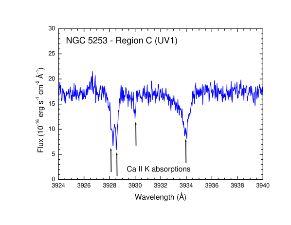
Figure 8: Ca II K $\lambda$3933 absorptions for region C of NGC 5253. Note the existence of several components. The wavelength axis has been corrected for the recession velocity of the galaxy. The two Galactic components are the bluest ones.

Although our main analysis of the spectra of NGC 5253 is focused on emission lines, we report the presence of some absorption features. They have been identified as Ca II K $\lambda$3933 and H $\lambda$3968, Mg I $\lambda$5167, Na I $\lambda\lambda$5890, 5896 and Ca II $\lambda\lambda$8498, 8662. The strongest absorption lines are Ca II H, K, which are unambiguously detected in all regions (see Figure 8 for the example of region C). We find that the Ca II H, K lines are splitted into several kinematical components (at least four), but two of them are due to Galactic absorption systems because of their low heliocentric radial velocity ($v_{rad}\sim$0 and $\sim$20 km s^-1, respectively).

The broader absorption component shows a radial velocity rather similar to that of the ionized gas of each region, and can be interpreted as the contribution of the stellar populations of NGC 5253. A second and narrower component with radial velocity $\sim$+95 km s^-1 is also detected in all regions. It might be of Galactic origin because NGC 5253 is located in the fourth quadrant of the Galaxy and radial velocities of the order of +100 km s^-1 are common. However, the relatively large galactic latitude, $b\sim+30^{\circ}$, makes rather unlikely its true Galactic nature. Other possibilities are that this absorption feature is produced by a relatively nearby high-velocity cloud or by an intergalactic cloud located at $\sim$1.3 Mpc. Using the formulae provided by Smoker et al. (2005), we find that the column density of this component is around 17 times smaller than that associated with NGC 5253.

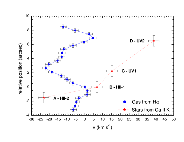
Figure 9: Position-velocity diagram of the H$\alpha$ emission line compared to the stellar component kinematics derived from the Ca II K absorption features observed in each region.

Data of radial velocities derived from the Ca II K absorption feature associated with NGC 5253 have been included in Figure 9 to compare the kinematics of the ionized gas with that of the stellar component. Notice that $v_{rad}$ determined from Mg I, Na I, and red Ca II absorptions detected in C and D are in good agreement with those derived from Ca II K. Although we only considered 4 points for constructing the position-velocity diagram of the absorption features, it is clear that gas and stars are kinematically decoupled. The stellar component seems to follow a behaviour consistent with a rotation pattern. If these velocity differences between gas and stars are due to the presence of a supershell, its velocity relative to the stellar velocity is $\sim$40–50 km s^-1. This value agrees with the expansion velocity of the supershell detected by Marlowe et al. (1995) in NGC 5253.

11 The age of the bursts and
the massive stellar population

Table 11: Analysis of O and WR populations in observed knots of NGC 5253.

	(A) HII-2	(B) HII-1	(C) UV-1	(D) UV-2
$F$ (WR Bump) (10-16 erg s-1 cm-2)	11 $\pm$ 3	10 $\pm$ 2	65 $\pm$ 18	1.2 $\pm$ 0.7
$L$ (WR Bump) (1036 erg s-1)	2.25 $\pm$ 0.66	2.01 $\pm$ 0.46	13.1 $\pm$ 3.6	0.24 $\pm$ 0.14
WNL eq. starsa	1.3 $\pm$ 0.4	1.2 $\pm$ 0.3	8 $\pm$ 2	0.14 $\pm$ 0.08
$L$ (H$\beta$) (1036 erg s-1)	271 $\pm$ 9	272 $\pm$ 8	204 $\pm$ 7	51.6 $\pm$ 1.9
O7V starsb	57 $\pm$ 2	57 $\pm$ 2	43 $\pm$ 1	10.8 $\pm$ 0.4
Adopted Age (Myr)	3.0 $\pm$ 0.1	2.7 $\pm$ 0.1	4.6 $\pm$ 0.1	5.1 $\pm$ 0.1
$\eta$c	$\sim$1.0	$\sim$1.1	$\sim$0.4	$\sim$0.3
O total stars	59 $\pm$ 2	51 $\pm$ 2	99 $\pm$ 5	36 $\pm$ 2
WR/(WR+O)	0.023 $\pm$ 0.007	0.023 $\pm$ 0.006	0.07 $\pm$ 0.03	0.004 $\pm$ 0.002

Although previous authors have derived the age of the last star-formation burst of NGC 5253, we have taken advantage of the high quality of our VLT spectra to make a reassessment of it through the H$\alpha$ equivalent width, $W$(H$\alpha$). We have used STARBURST99 (Leitherer et al., 1999) spectral synthesis models to estimate the age of each region, comparing the predicted H$\alpha$ equivalent widths with the observed values. We consider a spectral synthesis model with a metallicity of $Z$=0.008, the appropriate for NGC 5253, assuming an instantaneous burst with a Salpeter IMF, a total stellar mass of 10⁶ $M_{\odot}$ and a 100 $M_{\odot}$ upper stellar mass. The ages obtained are compiled in Table 11, and are in agreement with previous results.

In Figure 6 we can observe the broad emission feature of He II $\lambda$4686 originating from the stellar winds of WR stars, which is present in the four observed regions of NGC 5253. The He II $\lambda$4686 emission line is the most prominent feature of the so-called blue WR bump. Unfortunately, the existence of the red WR bump, that basically consists on the C IV $\lambda$5808 emission line, could not be studied because this spectral region is in our observational gap between 5783 and 5830 Å. In Figure 6 it is also evident the presence of broad emission features of N III $\lambda$4634 and N III $\lambda$4640, which are characteristic of WNL stars (Smith, Shara, & Moffat, 1996).

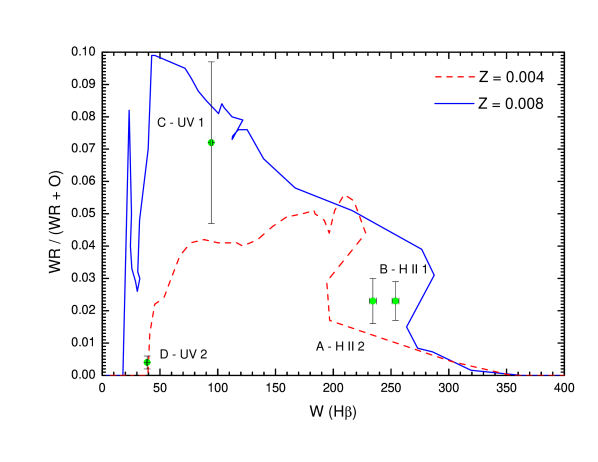
Figure 10: WR/(WR+O) versus W(H$\beta$) for Schaerer & Vacca (1998) models compared with our derived ratios.

We have used evolutionary synthesis models by Schaerer & Vacca (1998) for O and WR populations in young starburst to estimate the number of O and WR stars in the regions using the method explained in López-Sánchez, Esteban & Rodríguez (2004). We have assumed that all the flux of the blue WR bump comes from the broad He II $\lambda$4686 emission line (we show its extinction-corrected flux in Table 11) and a distance of 3.3 Mpc for NGC 5253. We only need 1 WNL star in regions A and B to produce the observed WR spectral features. The number of O stars was derived using the procedure given by Guseva, Izotov, & Thuan (2000) (their eq. 6). The derived number of O total stars and the WR/(WR+O) ratio are quoted in Table 11.

We have found a very good correspondence between our results and the predictions from Schaerer & Vacca (1998) models. In Figure 10 we plot the WR/(WR+O) ratio versus $W$(H$\beta$) for the models with $Z$=0.008 and 0.004. The metallicity of the analyzed regions inside NGC 5253 is $Z\sim$0.006 for A and B and $\sim$0.008 for C and D.

12 The localized nitrogen enrichment

As it was commented in §1, several authors have reported localized nitrogen enrichment in areas coincident with our regions A and B. Walsh & Roy (1989) and Kobulnicky et al. (1997) proposed that this localized enhancement is due to pollution by the winds of massive stars. However, for Kobulnicky et al. (1997) a difficulty of this hypothesis was the apparent lack of accompanying He enrichment in the zones where the N/H ratio is high. This fact was in contradiction with the observational and theoretical understanding of massive star yields. In this sense, the slightly higher He/H ratio we find in zones A and B with respect to C can solve somehow this puzzle. However, it must be taken into account that the detection of a modest helium pollution is difficult due to several reasons: a) the initial abundance of this element is far much higher than nitrogen, so the relative enrichment should be strong to be unambiguously detected; b) the uncertainty introduced by the assumed ICF to correct for the presence of neutral helium.

Our spectroscopic data include many more He I lines than previous works, our measurements have much higher signal-to-noise ratio, and we are using a more detailed method for determining the He⁺ abundance. For example, Kobulnicky et al. (1997) use a single line: He I $\lambda$5876, to determine the He⁺/H⁺ ratio. The intensity of that line is rather affected by collision and radiation transfer effects, and the calculations for correcting for these effects have improved since Kobulnicky et al. paper. In any case, the possible localized helium enrichment we detect is only marginal considering the quoted uncertainties. Unfortunately, it is clear that any result is necessarily unconclusive.

We have made a rough estimation of the mass of newly-created helium and nitrogen (stellar yield) necessary to produce the observed overabundances in regions A and B. We have reproduced the calculations of Kobulnicky et al. (1997) for obtaining the total ionizing mass of regions A and B, assuming the same angular size and filling factor, but considering a distance of 3.3 Mpc instead of the 4.1 Mpc assumed by those authors. In Table 12 we show the values we obtain for the cases of considering or not temperature fluctuations in the abundances, although the difference is almost irrelevant. We have considered the mean He and N abundances of regions A and B, and the yields are computed relative to the abundance of those elements in region C. Therefore, we have assumed that the initial abundance of NGC 5253 is that measured in region C and that zones A and B have suffered a localized and very recent increment of the He/H and N/H ratios. In Table 12 we have compared our empirical stellar yields with those obtained by Meynet & Maeder (2002) in their stellar evolution models including rotation. From the table, it can be seen that the contribution of a few evolved (WR) massive stars is enough to produce the observed pollution, in agreement with the low numbers of WNL stars estimated in §11 for zones A and B from the flux of the blue WR bump. The comparison with the also empirical yields determined by Esteban et al. (1992) for ring nebulae associated to Galactic WR stars gives further consistency to the hypothesis of the pollution by winds of WR stars. In particular, the similarity of the ratio of the He and N stellar yields estimated for NGC 5253 and for the other objects shown in Table 12 is the most remarkable fact of the table. That ratio is independent of the quite uncertain assumptions considered for deriving the empirical yields of the individual elements.

As it was commented in §8 and can be noted in Table 9, the O/H ratio in zone C is marginally higher that in zones A and B, (although the values can be considered similar taking into account the errors). It is interesting to note that nebular ejecta around WR stars (Esteban et al., 1992) and LBV stars (Smith et al., 1997; Lamers et al., 2001) show a substantial oxygen deficiency in their chemical content. This is also consistent with the scenario of pollution by evolved massive stars.

The presence of localized chemical enrichment in the youngest starburst of NGC 5253 indicates that the timescale of the process should be very short, as it was also suggested by Pustilnik et al. (2004). The similarity of the enrichment pattern observed in this galaxy and that of the Galactic WR ring nebulae (with estimated lifetimes of the order of 10⁴–10⁵ years, see Esteban et al. 1992) is another piece of evidence in the same direction. The most suitable scenario is that the pollution process is produced by the ejection of chemically enriched stellar external layers which are photoionized by the surrounding massive stars. This is, for example, the formation mechanism of the nebulae around luminous blue variables (LBVs), which also show a similar N enhancement (Smith et al., 1997; Lamers et al., 2001). In fact, Lamers et al. (2001) propose that the LBV nebulae are ejected during the blue supergiant phase of the progenitor star and that the chemical enrichment is due to rotation-induced mixing. Conversely, the observed pollution is rather unlikely to be produced by stellar wind material confined within a hot bubble. In this case, the timescale for mixing would be far much larger, of the order of $\sim$100 Myr (Tenorio-Tagle, 1996) because it should cool-down to temperatures of the order of the ionized gas.

Table 12: Comparison of empirical and theoretical stellar yields^a

			Contribution of stellar windsb
	NGC 5253 (A and B)		40 M⊙		60 M⊙	Galactic WR
Stellar yield	($t^{2}$=0)	($t^{2}$$>$0)	($v_{\rm rot}$=0)	($v_{\rm rot}$=300)	($v_{\rm rot}$=0)	Ring Nebulaec
$mp_{\rm N}$	0.03	0.04	0.002	0.026	0.015	0.002$-$0.02
$mp_{\rm He}$	5	7	0.2	4.1	2.1	0.2$-$3.6
$mp_{\rm He}$/$mp_{\rm N}$	167	175	100	158	140	90$-$180

13 About the origin of the abundance
discrepancy in NGC 5253

Very recently, Tsamis & Péquignot (2005) have proposed an explanation for the abundance discrepancy based on the implicit acceptation of the existence of temperature fluctuations but produced by a chemically inhomogeneous medium. These authors propose a chemically inhomogeneous model for 30 Doradus of low temperature and high metallicity embedded in a lower density medium of high temperature and low metallicity. The dense high metallicity regions come from Type II SN material that has not been mixed with the bulk of ISM and is in pressure balance with the normal composition ambient gas. These inclusions would be responsible for most of the emission in RLs with virtually no emission in CELs due to their very low electron temperature. We will present some objections to their models below.

Table 13: Comparison of the abundance discrepancy factor in different HII regions

		Galaxy		$R_{G}$a		ADF(O++)c	ADF(C++)d
Object	Galaxy	Type	MV	(kpc)	12+log(O/H)b	(dex)	(dex)	Referencee
M 16	Milky Way	Spiral	$-$20.9	6.34	8.56	0.45	$\cdots$	1
M 8				6.41	8.51	0.37	0.35	2
M 17				6.75	8.52	0.27	$\cdots$	2
					8.56	0.32	$\cdots$	3
M 20				7.19	8.53	0.33	$\cdots$	1
NGC 3576				7.46	8.56	0.24	$\cdots$	4
					8.52	0.32	$\cdots$	3
Orion nebula				8.40	8.51	0.14	0.40	5
					8.52	0.11	0.38	3
NGC 3603				8.65	8.46	0.29	$\cdots$	1
S 311				10.43	8.39	0.27	$\cdots$	6
NGC 5461	M 101	Spiral	$-$21.6	$\cdots$	8.56	0.29	$-$0.03/0.34	7
NGC 604	M 33	Spiral	$-$18.9	$\cdots$	8.49	0.20	$\cdots$	7
30 Doradus	LMC	Irregular	$-$18.5	$\cdots$	8.33	0.21	0.25	8
					8.34	0.30$-$0.43f	0.41	3
N11B				$\cdots$	8.41	0.69$-$0.91f	$\cdots$	3
N66	SMC	Irregular	$-$16.2	$\cdots$	8.11	0.36	$\cdots$	3
Region V	NGC 6822	Irregular	$-$16.0	$\cdots$	8.08	0.29	$\cdots$	9
NGC 2363	NGC 2366	Irregular	$-$18.2	$\cdots$	7.87	0.34	0.31:	7
Zones A and B	NGC 5253	BCDG	$-$17.2	$\cdots$	8.18	0.23	0.41g	10

First, the values of the abundance discrepancy factor (ADF) of O⁺⁺ (defined as the difference between the O⁺⁺ abundance determined from RLs and CELs) found for very different HII regions in different hosts galaxies are rather similar, as it can be seen in Table 13. In this table we show the ADF values determined for a sample of Galactic and extragalactic H II regions where the ADF of O⁺⁺ has been determined, their O/H ratio, the morphological type and absolute magnitude of the host galaxy and the Galactocentric distance in the case of the Galactic nebulae. It can be seen that the ADF is similar for most of the objects shown in the table, independently of the mass, type and metallicity of their host galaxy. The galaxies included in Table 13 have very different metallicities and gravitational potential wells and they should also have very different star formation histories and SN rates. In particular, in the case of NGC 5253, a high likelihood of a blow-out has been recently postulated by Summers et al. (2004). The energy injection rate into this galaxy due to the mechanical action of massive stars would seem sufficient to allow the expanding hot gas to escape its gravitational potential well. Moreover, the relatively small H I halo ($\sim$1.8 kpc along the minor axis) of this dwarf galaxy would also offer little resistance to this blow-out. The likelihood of past blow-outs suggests that the proposed delayed enrichment mechanism based on the rain of cooled-down droplets of SN ejecta would be less efficient in this galaxy, but this is not reflected in a lower value of the ADFs in NGC 5253 with respect to the other H II regions inside more massive galaxies. On the other hand, the Galactic H II regions studied in our sample are located at different galactocentric distances (from 6 to 11 kpc) in the Galactic disk. If the hypothesis of the enrichment by H-poor inclusions of SNe ejecta is correct, this would imply that this process is rather independent of the conditions and properties of the Galactic disk in such interval or radial distances.

Another important piece of evidence in this discussion is the fact that the ADF of C⁺⁺ in NGC 5253 (and other objects where this quantity has been determined, see Table 13) is rather similar to that of oxygen. We do not see any metallicity dependence of the relative importance of the ADF of C⁺⁺ with respect to that of O⁺⁺ in the objects where both quantities have been estimated (see Table 13). According to the model by Tsamis & Péquignot (2005), the overabundances in the metal rich regions amount to a factor of 8 in O and a factor of 14 in C. It is well known that massive star evolution models predict (e.g. Maeder 1992; Portinari, Chiosi, & Bressan 1998) that most of the net C is produced before the onset of the SN stage via stellar winds, and since the wind strength increases with metallicity, the C yield increases with metallicity. Carigi, Colín, Peimbert (2006) have produced a chemical evolution model for NGC 6822, a dwarf irregular galaxy of the Local Group, that predicts that only 36% of the C is due to massive stars that produce SN of type II, while 63% of the C is due to low and intermediate mass stars that do not produce Type II SN and, therefore, do not contribute to the C content of the droplets. Matteucci (2006) also finds that for the solar neighborhood most of the C is due to low and intermediate mass stars, while Carigi et al. (2005) find that about half of the C comes from intermediate mass stars and half from massive stars. Considering that the 30 Doradus chemical composition is similar to that of NGC 6822 V (see Table 13) one can reasonably infer that the expected overabundance of C should be lower than that of O, contrary to the assumptions of Tsamis & Péquignot (2005). Similarly, in the chemical evolution models most of the N is produced by low and intermediate mass stars and not by massive stars, consequently a considerable smaller overabundance of N than O is expected, contrary to the N and O values adopted in the model by Tsamis & Péquignot (2005).

14 Conclusions

We present deep echelle spectrophotometry in the 3100$-$10400 Å range of four selected zones of the nucleus of the blue compact dwarf galaxy NGC 5253. We have identified and measured a large number of emission lines in the spectra. This represents the largest collection of optical emission lines available for a dwarf starburst galaxy. Electron densities and temperatures have been consistently determined from a large number of emission line ratios of different ions. Chemical abundances of He, N, O, Ne, S, Cl, Ar, and Fe have been derived following standard methods. Recombination lines of C II and O II have been measured in the spectra of three of the individual zones analysed. The first time these kinds of lines have been unambiguously detected in a dwarf H II galaxy. The ionic abundances of C⁺⁺ and O⁺⁺ derived from these lines are from 0.20 to 0.40 dex larger than those determined from the intensity of collisionally excited lines. This behavior has been found in all the Galactic and extragalactic H II regions where both kinds of lines have been reported for the same ion. The quoted abundance differences can be accounted for a temperature fluctuations parameter ($t^{2}$) between 0.050 and 0.072.

The emission line profiles are complex and seem to be the combination of $-$at least$-$ two kinematical components with slightly different radial velocity and, in some zones, different line width. Apparently, there are no clear differences in the physical and chemical properties of the kinematical components, except perhaps a somewhat different reddening coefficient and N/O ratio in some particular zones. Position-velocity diagrams of different emission lines show a sinusoidal shape. However, the position-velocity diagram of stellar absorption spectral features shows a pattern entirely consistent with rotation. This fact suggests that the radial velocity behavor of the ionized gas should be due to outflows from the central starbursts and not a product of merging. We have derived the ages and the massive star population of the starburst. In particular, the detection of the so-called blue WR bump indicates the presence of a rather small number of WR stars in the starbursts.

Our observations confirm previous results that indicate the presence of localized N enrichment in two of the central starbursts of NGC 5253. Moreover, we also detect a possible slight He pollution in the same zones. The enrichment pattern is entirely consistent with that expected by the pollution of the winds of masive stars in the WR phase. Moreover, the estimated mass of newly created N and He is also consistent with the number of WR stars determined in the starbursts.

Finally, we conclude that a recent hypothesis that tried to solve the abundance discrepancy problem in H II regions in terms of a delayed enrichment by SNe ejecta inclusions (Tsamis & Péquignot, 2005) seems not to explain the available observational data in a satisfactory manner.

References

- Bautista & Pradhan (1996) Bautista, M.A., & Pradhan, A.K. 1996, A&A, 115, 551
- Beck et al. (1996) Beck, S.C., Turner, J.L., Ho, P.T.P., Lacy, J.H., & Kelly, D.M. 1996, ApJ, 457, 610
- Benjamin et al. (1999) Benjamin, R.A., Skillman, E.D., & Smits, D.P. 1999, ApJ, 514, 307
- Benjamin et al. (2002) Benjamin, R.A., Skillman, E.D., & Smits, D.P. 2002, ApJ, 569, 288
- Calzetti et al. (2004) Calzetti, D., Harris, J., Gallagher III, J.S., Smith, D.A., Conselice, C.J., Homeier, N. & Kewley, L. 2004, AJ, 127, 1405
- Campbell et al. (1986) Campbell, A., Terlevich, R., & Melnick, J. 1986, MNRAS, 223, 811
- Cardwell & Phillips (1989) Cardwell, N. & Phillips, M.M. 1989, ApJ, 338, 789
- Carigi et al. (2005) Carigi, L., Peimbert, M., Esteban, C. & García-Rojas, J. 2005, ApJ, 623, 213
- Carigi et al. (2006) Carigi, L., Colín, P., & Peimbert, M. 2006, ApJ, 644, 924
- De Robertis et al. (1987) De Robertis, Dufour, & Hunt 1987, JRASC, 81, 195
- D’Odorico et al. (2000) D’Odorico, S., Cristiani, S., Dekker, H., Hill, V., Kaufer, A., Kim, T., & Primas, F. 2000, Proc. SPIE, 4005, 121
- Esteban (2002) Esteban, C. 2002, RevMexAA Serie de Conferencias, in Ionized Gaseous Nebulae, a Conference to Celebrate the 60th Birthdays of Silvia Torres-Peimbert and Manuel Peimbert, W. J. Henney, J. Franco, M. Martos, & M. Peña (eds), 12, 56
- Esteban et al. (2005) Esteban, C., García-Rojas, J., Peimbert, M., Peimbert, A., Ruiz, M.T., Rodríguez, M., & Carigi, L. 2005, ApJ, 618, L95
- Esteban et al. (1998) Esteban, C., Peimbert, M., Torres-Peimbert, S. & Escalante, V. 1998, MNRAS, 295, 401
- Esteban et al. (2004) Esteban, C., Peimbert, M., García-Rojas, J., Ruiz, M.T., Peimbert, A., & Rodríguez, M. 2004, MNRAS, 355, 229
- Esteban et al. (1999a) Esteban, C., Peimbert, M., Torres-Peimbert, S., & García-Rojas, J. 1999a, Rev. Mex. AA, 35, 65
- Esteban et al. (1999b) Esteban, C., Peimbert, M., Torres-Peimbert, S., García-Rojas, J., & Rodríguez, M. 1999b, ApJS, 120, 113
- Esteban et al. (2002) Esteban, C., Peimbert, M., Torres-Peimbert, S., & Rodríguez, M. 2002, ApJ, 581, 241
- Esteban et al. (1992) Esteban, C., Vílchez, J. M., Smith, L. J., & Clegg, R. E. S. 1992, A&A, 259, 629
- García-Rojas et al. (2004) García-Rojas, J., Esteban, C., Peimbert, M., Rodríguez, M., Ruiz, M.T. & Peimbert, A. 2004, ApJS, 153, 501
- García-Rojas et al. (2005) García-Rojas, J., Esteban, C., Peimbert, A., Peimbert, M., Rodríguez, M. & Ruiz, M.T. 2005, MNRAS, 362, 301
- García-Rojas et al. (2006) García-Rojas, J., Esteban, C., Peimbert, M., Costado, M.T., Rodríguez, M., Peimbert, A., & Ruiz, M.T. 2006, MNRAS, 368, 253
- Garnett (1992) Garnett, D.R. 1992, AJ, 103, 1330
- Garnett et al. (1999) Garnett, D.R., Shields, G.A., Peimbert, M., Torres-Peimbert, S., Skillman, E.D., Dufour, R.J., Terlevich, E. & Terlevich, R.J. 1999, ApJ, 513, 168
- Gibson et al. (2000) Gibson, B.K. et al. 2000, ApJ, 529, 723
- Guseva et al. (2000) Guseva, N., Izotov, Y. I. & Thuan, T.X. 2000, ApJ, 531, 776
- Howarth & Murray (1990) Howarth I.D. & Murray J. 1990, SERC Starlink User Note No. 50
- Izotov et al. (1994) Izotov, Y.I., Thuan, T.X., & Lipovetski, 1994, ApJ, 435, 647
- Kingdon & Ferland (1995) Kingdon, J. & Ferland, G.J. 1995, ApJ, 442, 714
- Kobulnicky & Skillman (1995) Kobulnicky, H.A, & Skillman, E.D. 1995, ApJ, 454, L121
- Kobulnicky et al. (1997) Kobulnicky, H.A., Skillman, E.D., Roy, J.-R., Walsh, J.R. & Rosa, M.R., 1997, ApJ, 277, 679
- Lamers et al. (2001) Lamers, H. J. G. L. M., Nota, A., Panagia, N., Smith, L. J., Langer, N. 2001, ApJ, 551, 764
- Leitherer et al. (1999) Leitherer, C., Schaerer, D., Goldader, J.D., González-Delgado, R.M., Robert, C., Kune, D.F., de Mello, D.F., Devost, D. & Heckman, T.M. 1999, ApJS, 123, 3
- López-Sánchez et al. (2004) López-Sánchez, .R., Esteban, C. & Rodríguez, M. 2004, ApJS, 153, 243
- López-Sánchez et al. (2006) López-Sánchez, Á.R., Esteban, C. & García-Rojas, J. 2006, A&A, 449, 997
- Maeder (1992) Maeder, A. 1992, A&A, 264, 105
- Marlowe et al. (1995) Marlowe, A.T., Heckman, T.M, Wyse, R.F.G., & Schommer, R. 1995, ApJ, 438, 563
- Martin & Kennicutt (1995) Martin, C.L. & Kennicutt, R.C., Jr, 1995, ApJ, 447, 171
- Martín-Hernández, Schaerer, & Sauvage (2005) Martín-Hernández, N.L., Schaerer, D., & Savage, M. 2005, A&A, 429, 449
- Mathis & Rosa (1991) Mathis, J.S., & Rosa, M.R. 1991, A&A, 245, 625
- Matteucci (2006) Matteucci, F. 2006, in Origin of Matter and Evolution of Galaxies - New Horizon of Nuclear Astrophysics and Cosmology, ed. S. Kubono, astro-ph/0603820
- Mazzarella & Boroson (1993) Mazzarella, J.M. & Boroson, T.A. 1993, ApJS, 85, 27
- Meier et al. (2002) Meier, D.S., Turner, J.L., & Beck, S.C. 2002, AJ, 124, 877
- Méndez & Esteban (1997) Méndez, D.I. & Esteban, C. 1997, ApJ, 488, 652
- Méndez & Esteban (1999) Méndez, D.I. & Esteban, C. 1999, AJ 118, 2733
- Mendoza (1983) Mendoza, C., 1983, Flower, D.R., Reidel, D., eds. Proc. IAU Symp. 103, Planetary Nebulae, Kluwer, Dordrecht, 143
- Meynet & Maeder (2002) Meynet, G. & Maeder, A. 2002, A&A, 390, 561
- Moorwood & Glass (1982) Moorwood, A.F.M. & Glass, I.F. 1982, A&A, 115, 84
- Moore et al. (2004) Moore, Hester, & Dufour 2004 AJ, 127, 3484
- Péquignot et al. (2002) Péquignot, D., Amara, M., Liu, X.-W., Barlow, M. J., Storey, P. J., Morisset, C., Torres-Peimbert, S., Peimbert, M., 2002, RevMexConfSer, 12, 142
- Peimbert (2003) Peimbert, A. 2003, ApJ, 584, 735
- Peimbert et al. (2002) Peimbert, A., Peimbert, M. & Luridiana, V. 2002, ApJ, 565, 688
- Peimbert et al. (2005) Peimbert, A. Peimbert, M., & Ruiz, M.T. 2005, 634, 1056
- Peimbert (1967) Peimbert, M. 1967, ApJ, 150, 825
- Peimbert & Costero (1969) Peimbert M. & Costero, R. 1969, Bol. Obs. Tonantzintla y Tacubaya, 5, 3
- Peimbert & Torres-Peimbert (1977) Peimbert, M., & Torres-Peimbert. S. 1977, MNRAS, 179, 217
- Peimbert et al. (1992) Peimbert, M., Torres-Peimbert, S., & Ruiz, M.T. 1992, Rev. Mex. Astron. Astrofís., 24, 155
- Peimbert et al. (2000) Peimbert, M., Peimbert, A., & Ruiz, M.T. 2000, ApJ, 541, 688
- Portinari et al. (1998) Portinari, L., Chiosi, C., & Bressan, A. 1998, A&A, 334, 505.
- Pustilnik et al. (2004) Pustilnik, S., Kniazev, A., Pramskij, A., Izotov, Y., Foltz, C., Brosch, N., Martin, J.-M. & Ugryumov, A., 2004, A&A, 419, 469
- Quinet (1996) Quinet, P. 1996, A&AS, 116, 573
- Rieke et al. (1988) Rieke, G.H., Lebofsky, M.J., & Walker, C.E., 1988, ApJ, 325, 679
- Rodríguez (1996) Rodríguez, M. 1996, A&A, 313, L5
- Rodríguez (1999) Rodríguez, M. 1999, A&A, 348, 222
- Rodríguez (2002) Rodríguez, M. 2002, A&A, 389, 567
- Rodríguez & Rubin (2005) Rodríguez, M. & Rubin, R.H. 2005, ApJ, 626, 900
- Ruiz et al. (2003) Ruiz, M.T., Peimbert, A., Peimbert, M., & Esteban, C. 2003, ApJ, 595, 247
- Sawey & Berrington (1993) Sawey, P.M.J. & Berrington, K.A. 1993, At. Data Nucl. Data Tables, 55, 81
- Schaerer et al. (1997) Schaerer, D. Contini, T., Kunth, D., & Meynet, G. 1997, ApJ, 481, L75
- Schaerer & Vacca (1998) Schaerer, D. & Vacca, W. C. 1998, ApJ, 497, 618
- Schweizer (1982) Schweizer, F. 1982, ApJ, 252, 455
- Seaton (1979) Seaton, M. J., 1979, MNRAS, 187, 73
- Shaw & Dufour (1995) Shaw, R.A. & Dufour, R.J. 1995, PASP, 107, 896
- Skillman et al. (1989) Skillman, E. D., Kennicutt, R. C. & Hodge, P. W. 1989, ApJ, 347, 875
- Smits (1996) Smits, D.P. 1996, MNRAS, 278, 683
- Smith et al. (1996) Smith, L. F., Shara, M. M. & Moffat, A. F. J. 1996, MNRAS, 281, 163
- Smith et al. (1997) Smith, L. J., Stroud, M. P., Esteban, C., & Vílchez, J. M. 1997, MNRAS, 265, 265
- Smoker et al. (2005) Smoker, J.V., Keenan, F.P., Thompson, H.M.A., Brüns, C., Muller, E., Lehner, N., Lee, J.-K. & Hunter, I. 2005, A&A, 443, 525S
- Stasińska (1978) Stasińska, G. 1978, A&A, 66, 257
- Stasińska (1990) Stasińska, G. 1990, A&AS, 83, 501
- Storey & Hummer (1995) Storey, P. J., & Hummer, D. G., 1995, MNRAS, 272, 41
- Strickland & Stevens (2000) Strickland, D.K. & Stevens, I.R. 2000, MNRAS, 314, 511
- Summers et al. (2004) Summers, L.K., Stevens, I.R., Strickland, D.K., & Heckman, T.M. 2004, MNRAS, 351, 1
- Tenorio-Tagle (1996) Tenorio-Tagle, G. 1996, AJ, 111, 1641
- Thim et al. (2003) Thim, F., Tammann, G.A., Saha, A., Dolphin, A., Sandage, A., Tolstoy, E. & Labhardt, L. 2003, ApJ, 590, 256
- Torres-Peimbert et al. (1980) Torres-Peimbert, S., Peimbert, M. & Daltabuit, E. 1980, ApJ, 238, 133
- Tremonti et al. (2001) Tremonti, C.A., Calzetti, D., Leitherer, C. & Heckman, T.M. 2001, ApJ, 555, 322
- Tsamis et al. (2003) Tsamis, Y.G., Barlow, M.J., Liu, X.-W., Danziger, I.J., & Storey, O.J., 2003, MNRAS, 338, 687
- Tsamis et al. (2004) Tsamis, Y.G., Barlow, M.J., Liu, X.-W., Storey, P.J. & Danziger, I.J. 2004, MNRAS, 353, 953
- Tsamis & Péquignot (2005) Tsamis Y. G., Péquignot D. 2005, MNRAS, 364, 687
- Turner et al. (1997) Turner, J.L., Beck, S.C., & Hurt, R.L. 1997, ApJ, 474, L11
- Vacca & Conti (1992) Vacca, W.D. & Conti, P.S., 1992, ApJ, 401, 543
- van den Bergh (1980) van den Bergh, S. 1980, PASP, 92, 122
- Verner et al. (2000) Verner, E.M., Verner, D.A., Baldwin, J.A., Ferland, G.J., & Martin, P.G. 2000, ApJ, 543, 831
- Véron et al. (1997) Véron, P., Gonçalves, A.C. & Véron-Cetty, M.-P. 1997, A&A, 319, 52
- Walsh & Roy (1987) Walsh, J.R., & Roy, J.-R., 1987, ApJ, 319, L57
- Walsh & Roy (1989) Walsh, J.R., & Roy, J.-R., 1989, MNRAS, 239, 297
- Welch (1970) Welch, G.A. 1970, ApJ, 161, 821
- Zhang (1996) Zhang, H. L. 1996, A&AS, 119, 523