On the narrowband detection properties of high-redshift Lyman-alpha emitters

Abstract

Context. Numerous surveys are currently underway or planned that aim to exploit the strengths of the Lyman-alpha emission line for cosmological purposes. Today, narrowband imaging surveys are frequently used as a probe of the distant universe.

Aims. To investigate the reliability of the results of such high-$z$ Ly$\alpha$ studies, and the validity of the conclusions that are based upon them. To determine whether reliable Ly$\alpha$ fluxes ($F_{{\rm Ly}\alpha}$) and equivalent widths ($W_{{\rm Ly}\alpha}$) can be estimated from narrowband imaging surveys and whether any observational biases may be present.

Methods. We have developed software to simulate the observed line and continuum properties of synthetic Ly$\alpha$ galaxies in the distant universe by adopting various typical observational survey techniques. This was used to investigate how detected $F_{{\rm Ly}\alpha}$ and $W_{{\rm Ly}\alpha}$ vary with properties of the host galaxy or intergalactic medium: internal dust reddening; intervening Ly$\alpha$ absorption systems; the presence of underlying stellar populations.

Results. None of the techniques studied are greatly susceptible to underlying stellar populations or the relative contribution of nebular gas. We find that techniques that use one off-line filter on the red side of Ly$\alpha$ result in highly inaccurate measurements of $W_{{\rm Ly}\alpha}$ under all tests. Adopting two off-line filters to estimate continuum at Ly$\alpha$ is an improvement but is still unreliable when dust extinction is considered. Techniques that employ single narrow- and broad-band filters with the same central wavelength are not susceptible to internal dust, but Ly$\alpha$ absorption in the IGM can cause $W_{{\rm Ly}\alpha}$ to be overestimated by factors of up to 2: at $z=6$, the median $W_{{\rm Ly}\alpha}$ is overestimated by $\sim 25$%. The most robust approach is a SED fitting technique that fits $E_{B-V}$ and burst-age from synthetic models – broadband observations are needed that sample the UV continuum slope, 2175Å dust feature, and the 4000Å discontinuity. We also notice a redshift-dependent incompleteness that results from DLA systems close to the target LAEs, amounting to $\sim 10$% at $z=6$.

1 Introduction

Galaxies hosting young, violent starbursts are expected to accommodate numerous massive, hot stars that are bright in the far ultraviolet (UV) regime. UV photons with wavelengths shortwards of the Lyman break ionise their local interstellar media (ISM), resulting in recombination nebulae bright in hydrogen lines. Two-thirds of the Lyman-continuum photons are reprocessed as Lyman-alpha (Ly$\alpha$) under the assumption of case B recombination, and it could be expected that young starburst regions should be consistently Ly$\alpha$-bright.

Early observations of local star-forming galaxies with the International Ultraviolet Explorer (IUE) demonstrated this not to be the case. In small samples of relatively un-evolved galaxies (low dust and metal content) Ly$\alpha$ was frequently shown to be absent or unexpectedly weak (eg. Meier & Terlevich ref:meier82 (1982); Hartmann et al. ref:hartmann88 (1988); Calzetti & Kinney ref:calkin92 (1992)). Although dust could be invoked to explain the absence of this FUV emission line, Giavalisco et al. (ref:giavalisco96 (1996)) demonstrated that pure dust extinction could not explain the weak Ly$\alpha$ fluxes from any of the galaxies in the IUE samples. Instead results suggest that Ly$\alpha$ photons have decoupled from the non-resonant continuum radiation, resulting in line-photons escaping the host over significantly extended path-lengths; thereby increasing their sensitivity to dust (Neufeld ref:neufeld90 (1990)). On the other hand, Neufeld (ref:neufeld91 (1991)) also found that resonance scattering can cause less attenuation of Ly$\alpha$ photons compared to continuum if the ISM is multiphase: if dusty, neutral clouds are embedded in a dust-free, ionised ISM, resonance scattering can reflect Ly$\alpha$ photons from the surface of the clouds, allowing them to diffuse out of the ISM relatively unattenuated. Radiative transport in such multiphase, clumpy media has more recently been studied by Hansen & Oh (ref:hansen05 (2005)) who found Ly$\alpha$ equivalent widths ($W_{{\rm Ly}\alpha}$) could be ‘boosted’ by factors of $2-3$.

In the local universe, the observational situation was further-complicated by Ly$\alpha$ spectroscopic observations using the Goddard High-Resolution Spectrograph (GHRS) and Space Telescope Imaging Spectrograph (STIS) both onboard Hubble Space Telescope (HST). In a sample of 8 local starbursts, Kunth et al. (ref:kunth98 (1998)) found that when Ly$\alpha$ is seen in emission, blueshifted Ly$\alpha$ absorption features are also common, leading to P-Cygni-like profiles. In the same study, O i and Si ii UV absorption lines were also blueshifted with respect to the ionised gas, indicating large-scale outflows of the ISM with velocities up to 200 km s^-1. Mas-Hesse et al. (ref:mas-hesse03 (2003)) demonstrated that varying Ly$\alpha$ profiles from starbursts are well explained by an evolutionary super-shell model; over the lifetime of a starburst, absorption, pure emission, and P-Cygni emission phases will all be observed, depending on the properties of the outflow and viewing angle. If Ly$\alpha$ escape is associated with winds and photons can diffuse through H i, low surface brightness Ly$\alpha$ emission may be expected to span large areas, significantly more extended than the starburst itself as probed by FUV emission. Hence imaging becomes an efficient method by which the line can be isolated. This was the motivation for our HST survey using the Advanced Camera for Surveys (ACS; Kunth et al. ref:kunth03 (2003)). Such Ly$\alpha$ imaging studies are extremely sensitive to how the continuum is subtracted and much supporting data is required in order to estimate the continuum flux at Ly$\alpha$. We found in Hayes et al. (ref:hayes05 (2005)) that at least three off-line imaging observations are necessary in order to estimate the continuum flux at Ly$\alpha$. We determined it necessary to sample the UV continuum slope and 4000Å break in order to disentangle the effects of age and reddening, allowing us to estimate the flux due to continuum processes in the on-line filter from synthetic models. In our sample, luminous blue compact galaxy ESO 338-IG04 shows regions of diffuse Ly$\alpha$ emission spanning several kpc, and patchy structure consistent with an inhomogeneous and outflowing ISM. In the diffuse regions $W_{{\rm Ly}\alpha}$ is shown to be very large $(>200\AA)$ where continuum flux is weak, but integrated over the whole galaxy $W_{{\rm Ly}\alpha}$ is $\sim 20$Å, an order of magnitude lower. Damped absorption with $W_{{\rm Ly}\alpha}$$\sim-40$Å is also observed in some central regions, demonstrating the sensitivity of Ly$\alpha$ to small-scale variations in the ISM.

Due to its sensitivity to star-forming activity, high natural equivalent widths (up to 240Å; Charlot & Fall ref:cf93 (1993)) sensitivity to dust, and convenient spectral positioning in the FUV, Ly$\alpha$ has long been considered a competitive tracer of primeval high-$z$ galaxies as they form their first generation of stars. Partridge & Peebles (ref:pp67 (1967)) suggested that in a collapsing H i halo, as much as 7% of the gravitational energy could be radiated in the Ly$\alpha$ line. While surveys that target continuum emission or utilise dropout techniques may have been highly successful in recent years, they all share one common weakness: a luminosity bias in favour of galaxies with strong continuum. Such a bias leads to incompleteness at low luminosity and these surveys would miss the numerous low-mass, star-forming objects; the dominant species in the paradigm of hierarchal galaxy formation.

The early days of high-$z$ Ly$\alpha$ studies were largely unsuccessful (see Pritchet ref:prit94 (1994) for a review) and it was not until the late 1990’s that searches for high-$z$ Ly$\alpha$-emitters (LAE) became fruitful. Despite the complications, high-$z$ Ly$\alpha$-emitting objects are now routinely being discovered by imaging techniques (Cowie & Hu ref:cowiehu98 (1998); Rhoads et al. ref:rhoads00 (2000); Fynbo et al. ref:fynbo03 (2003); Kodaira et al. ref:kodaira03 (2003); Yamada et al. ref:yamada05 (2005)), fields surrounding massive objects (eg. Monaco et al. ref:monaco05 (2005)), and spectroscopic observations (eg. Kurk et al. ref:kurk04 (2004)). After much initial disagreement, the predicted and observed luminosity functions (LF) of LAEs at high-$z$ may be converging (Le Delliou et al. ref:ledelliou05 (2005)). Interestingly however, a fraction of the LAEs uncovered in the high-$z$ universe have very large measured equivalent widths (Cowie & Hu ref:cowiehu98 (1998); Malhotra & Rhoads ref:malrhoads02 (2002)). In the case of Malhotra & Rhoads (ref:malrhoads02 (2002)), their LAE population at $z=4.5$ was shown to have a median $W_{{\rm Ly}\alpha}$ of 400Å, 65% greater than the maximum value of 240Å (Charlot & Fall, ref:cf93 (1993)) that can be generated by pure star-formation models with normal metallicities and IMFs. These authors interpreted this to imply that either these objects were type II quasars or star-forming galaxies with very top-heavy IMFs or zero-metallicity stars. Subsequent X-ray observations with the Chandra satellite ruled out the possibility that these objects could be AGN (Wang et al. ref:wang04 (2004)). Jimenez & Haiman (ref:jimenez06 (2006)) demonstrate how this (and other effects) can be explained if 10-30% of the stars in these galaxies are primordial. ‘Normal’ starburst conditions could still explain such high equivalent widths but the system would have to be perfectly configured so as to allow Ly$\alpha$ photons to leak out while dust blocks much of the stellar UV radiation. Another possibility is that this is the result of some other astrophysical effect, external to the host galaxy that may cause certain observational techniques to overestimate $W_{{\rm Ly}\alpha}$ when such narrowband imaging techniques are used.

While Ly$\alpha$ may provide a ‘clean’ probe of the high-$z$ universe, the common observational trade-off is evident: spectroscopic studies may be rich in information regarding the line, while narrowband imaging studies may be efficient for detections. Future generations of high-$z$-optimised integral field units (eg. the Multi Unit Spectroscopic Explorer (MUSE) bound for ESO’s VLT) have the potential to provide significant advances in this area. However, in the cases where narrowband imaging alone is used to derive information about the line, it is essential to examine exactly how efficient the technique is in doing so. To our knowledge, no such comprehensive study has previously been performed and this article represents the first step in doing so. We here simulate how various survey techniques may estimate Ly$\alpha$ detection properties – line flux ($F_{{\rm Ly}\alpha}$) and equivalent width ($W_{{\rm Ly}\alpha}$) – of galaxies at high-$z$.

The paper is organised as follows: in Sect. 2 we describe the software; in Sect. 3 we present the simulations we have performed; in Sect. 4 we present and discuss some of the more important results; and in Sect. 5 we present our concluding remarks. We assume a flat cosmology with $\Omega_{\mathrm{M}}=0.3$, $\Omega_{\Lambda}=0.7$, $H_{0}=70$ km s^-1 Mpc^-1 throughout.

2 The software

The Ly$\alpha$ galaxy simulation software follows a simple three-step prescription: (i) the restframe spectral energy distribution (SED) of a the test galaxy is generated and the Ly$\alpha$ line is added; (ii) the SED is redshifted and the effects of intervening material (IGM absorption) are applied to the spectrum; and (iii) the spectrum is convolved with various filter response profiles and fluxes are computed.

2.1 SED generation

Restframe SEDs of starburst galaxies are generated from the Starburst99 (hereafter SB99; Leitherer et al. ref:leitherer99 (1999); Vázquez & Leitherer ref:vazlei04 (2004)) synthetic spectral models. No nebular emission lines are thought to be strong enough to significantly contribute to fluxes in the UV filters considered here (see Sect. 2.3 for a description of the filters) – filters are broad and continuum dominated, and in Hayes et al. (ref:hayes05 (2005)) we concluded that optical emission lines had negligible impact upon our study. Hence the SB99 spectra are used unmodified, free of nebular emission lines but including nebular continuum emission. The software was designed for flexibility and to cover as wide parameter space as possible, enabling the user to perform a wide array of parameter dependency tests. Spectra can be selected from the 1999 SB99 data-release, choosing with burst modes (instantaneous or continuous), composition (stellar-only or stellar+nebular), metallicity, initial mass function, and age. In addition to the standard set of spectra, SED modification code was written to allow the selection of:

1. Departures from the single stellar population (SSP). It is well known from studies of the low- and high-$z$ universe that star-forming galaxies often exhibit composite spectra, with contributions from the current starburst and an underlying, older stellar population. Our method for testing the effects of such population mixing is to allow any single SB99 spectrum to act as a template for a secondary population. This secondary spectrum is renormalised so it contributes a specified fraction of the spectrum under consideration at a user-specified wavelength, and is added to the spectrum or set of spectra.

2. Variations in the contribution of nebular gas. By subtracting out the nebular component from corresponding pairs of spectra, the nebular gas spectrum as a function of age is recovered. The gas spectrum can then be re-scaled and added back to the stellar-only component. Thus a normalisation factor of 0 corresponds to a stellar-only spectrum, 1 corresponds to the standard stellar+nebular spectrum, and factors $>1$ imply the gas spectrum has been boosted.

Restframe spectra are rebinned to 1Å steps in wavelength. After generation of the template spectrum, the whole SED is renormalised to $L_{\lambda}$ at 1500Å based upon input star-formation rate ($SFR$) using the relationship

$$L_{\lambda}(1500\mbox{\AA})=9.5238\times 10^{39}SFR(\mbox{M}_{\sun}\mbox{yr}^{-1})$$ (1)

adapted from Kennicutt (ref:kenn98 (1998)). The all-important Ly$\alpha$ line of specified equivalent width is added to the spectrum at wavelength of 1216Å. At the rest wavelength of Ly$\alpha$, 1Å corresponds to the velocity of 250 km s^-1. In addition, pure imaging studies aren’t sensitive to line profiles and our aim is simply to investigate how well intrinsic line-strengths are recovered (whatever their origin or profile). Hence all the energy is deposited in one 1Å bin. See Sect. 2.3 for a more detailed discussion of this.

Ly$\alpha$ is the only Lyman series feature added to the SED – the O vi–Ly$\beta$–C ii complex between 1032 and 1038Å does not fall within any of the filter bandpasses considered here (Sect. 2.3). The C iv$\lambda$1549Å absorption feature (although frequently observed with P-Cygni profiles), common in star-forming galaxies, does fall centrally in one of the bandpasses we use. In a sample of 45 local galaxies observed with the IUE, Heckman et al. (ref:heckman98 (1998)) find a (C iv+Si iv)/2 median equivalent width of -4.6Å, with the absorption features never stronger than -10.1Å. Crowther et al. (ref:crowther06 (2006)) re-measured these equivalent widths, finding an offset of 1-2Å relative to the Heckman et al. result. The filter bandpass that the C iv feature falls in is broad ($(1+z)\cdot 300$Å, centred at 1500Å; see Sect. 2.3) so the presence of the strongest locally observed C iv feature would affect the integrated flux by only $\sim 3$% with no redshift dependence. Moreover, these authors found that this equivalent width is positively correlated with metallicity. Since strong Ly$\alpha$ emission is often interpreted as a sign of low-metallicity stars, we decided not to apply the C iv feature to our SEDs.

In order to complete the restframe SED, it can be reddened using the Galactic laws of Seaton (ref:seaton79 (1979)), or Cardelli et al. (ref:ccm89 (1989)), the SMC law fit of Prévot et al. (ref:prevot84 (1985)), the LMC law of Fitzpatrick et al. (ref:fitz85 (1985)), and the Starburst law of Calzetti et al. (ref:calzetti00 (2000)).

2.2 Effects of cosmic distance

The restframe SED is first shifted to the desired redshift and the luminosity distance $d_{\mathrm{L}}$ computed from the formula

$$d_{\mathrm{L}}=(1+z)\frac{c}{H_{0}}\int_{0}^{z}\frac{dz^{\prime}}{\sqrt{\Omega_{\mathrm{M}}(1+z^{\prime})^{3}+\Omega_{\Lambda}}}$$ (2)

where $H_{0}$ is the Hubble constant and $\Omega_{\mathrm{M}}$ and $\Omega_{\Lambda}$ are the energy densities of total matter and cosmological constant, respectively. The luminosity at each wavelength is then converted to flux using the inverse square law.

Given that we want to study all the possible astrophysical effects, including possible extreme cases, we chose to treat the effects of intervening H i clouds by generating random distributions of individual clouds, not by applying some general average prescription (eg. Madau ref:madau95 (1995)). The effect of intervening H i clouds (Ly$\alpha$ forest (LAF) to damped Ly$\alpha$ (DLA) systems) is implemented by first assuming the number density of absorbing clouds as a function of redshift takes the form of the power-law $N(z)=N_{0}(1+z)^{\gamma}$ in the redshift range 0 to $z$ where $N_{0}=0.07^{+0.13}_{-0.04}$ and $\gamma=2.45^{+0.75}_{-0.65}$ (Peroux et al. ref:peroux03 (2003)). Firstly the total number of clouds in the given redshift range is generated by biasing a uniform variate pseudo-random number (PRN) by the distribution function, within the observational constraints. For each cloud, a position in redshift space is generated in the same manner: by weighting a PRN by the distribution function. The column density $(n_{\mathrm{HI}})$ of each cloud is generated by assuming the distribution obeys the power-law $N(n_{\mathrm{HI}})\propto n_{\mathrm{HI}}^{-\beta}$ (Rao et al. ref:rao05 (2005)) for $\beta=1.4\pm 0.2$ and column densities in the range $13\leq\log(n_{\mathrm{HI}}[\mathrm{cm^{-2}]})\leq 22$.

Once the redshift–column-density distribution is generated, the effect on the SED of each cloud is determined from its equivalent width in absorption ($W_{\mathrm{abs}}$). We compute restframe $W_{\mathrm{abs}}$ from the effective optical depth at line-centre ($\tau_{0}$) following the curve of growth method (Spitzer ref:spitzer78 (1978)). After cosmological scaling $(1+z_{\mathrm{cloud}})$, $W_{\mathrm{abs}}$ and the continuum flux-density at $(1+z_{\mathrm{cloud}})\cdot\lambda_{\mathrm{Ly\alpha,0}}$ are then used to remove the requisite amount of flux from the appropriate bins in the redshifted spectrum. In cases where the absorption is damped ($W_{\mathrm{abs}}$ is greater than the bin size), the flux in that bin is set to zero and flux is symmetrically removed from neighbouring bins until the required $W_{\mathrm{abs}}$ has been met.

Significant attention has been paid to the possibility of reddening of high-$z$ quasar spectra by DLA systems (eg. Pei, Fall & Bechtold ref:pei91 (1991)). However, recent studies have demonstrated the typical mean cumulative reddening from DLA systems to be small. For example Ellison, Hall & Lira (ref:ellison:05 (2005)) found mean $E_{B-V}<0.04$ at the $3\sigma$ level for SMC-type dust in a sample of 14 high-$z$ quasars with DLAs, while from a sample of 72 DLA quasars from the Sloan Digital Sky Survey, Murphy & Liske (ref:murphy04 (2004)) found mean $E_{B-V}<0.02$ at $3\sigma$ for SMC dust. On the other hand, Wild et al. (ref:wild06 (2006)) find evidence for significant reddening in Ca ii and Mg ii absorbing systems: $E_{B-V}=0.105$ for SMC type dust in the selected strongest absorbers ($E_{B-V}=0.066$ for their complete sample). Such objects are shown to be similar to DLAs with a number density of $\sim 20$–30% that of DLAs at the same redshift. While we do not claim that some high-$z$ LAEs would not be heavily dust reddened, we chose for this part of the study not to implement dust-reddening by high-H i column-density systems.

At $z=0$, the redshifted SED can be reddened once more using the laws of Cardelli et al. (ref:ccm89 (1989)) or Seaton (ref:seaton79 (1979)) to simulate Milky-Way reddening.

2.3 Filters and computation of line fluxes and equivalent widths

For the sake of simplicity (our aim was to study astrophysical processes, not observational complexities) the filters are perfect. Defined only by their central wavelength and effective width, they provide 100% transmission inside the passband and zero otherwise. That is, the filters are as close to perfect top-hats as possible, without introducing numerical, resolution-dependent inconsistencies at the edges. Narrowband filters targeting the Ly$\alpha$ line are defined to have a full width of 2% their central wavelength $(\lambda_{\mathrm{c}})$ while broadband filters have full widths of 20% $\lambda_{\mathrm{c}}$. That is, the width of the broadband filters scales with $\lambda_{\mathrm{c}}$ in approximately the same way as it does in the Johnson-Cousins/Bessell and JHKLM systems. The narrowband filters scale similarly so as not to introduce effects that may result from sampling different spectral regions at different redshifts.

One issue that arises when using narrow filters to isolate an emission line is the positioning of the line within the filter profile. That is, is the line centrally positioned and narrow enough to allow maximum transmission of the line flux? Chemistry and manufacturing processes dictate that filters (particularly narrowband) cannot be perfectly rectangular and most frequently take the form of bell-curves. Whilst photometric redshifts or drop-out techniques may be used to remove interlopers (most notably [O ii]$\lambda 3726$Å), photo-$z$’s of individual objects do not reach the required levels of accuracy to determine the position of Ly$\alpha$ within a narrow bandpass (typical photo-$z$ accuracies of $\Delta z=0.05(1+z)$ cannot determine whether the line falls within a 2%$\lambda_{\mathrm{c}}$ narrowband filter or not). In addition, photo-$z$ methods tend to be reliant upon sampling the Balmer/4000Å break which is lost from optical multiband datasets at $z\sim 1$, something we discuss in another context in Sect. 4. At high-$z$ and without spectroscopic data, the selection of LAE candidates by detection in the narrowband filter becomes the most accurate estimate of redshift. Hence effects that result from the line falling in the wing of a filter will always be something that has to be considered. Starburst galaxies do not exhibit significantly broadened spectral lines: concerning Ly$\alpha$, Matsuda et al. (ref:matsuda06 (2006)) spectroscopically measured the widths of 37 LABs at $z=3.1$, finding Ly$\alpha$ full widths (FWHM) in the range 150-1700 km s^-1 with a median value of 550 km s^-1. This corresponds to a maximum Gaussian $\sigma$ of 3Å at Ly$\alpha$ (median value of $\sim 1$Å). Thus given the 2%$\lambda_{\mathrm{c}}$ narrowband filters used here, even the broadest Ly$\alpha$ lines will be completely transmitted (2% rectangular filters drop to 99% of complete line transmission at $\sigma=4.70\AA\ \sim FWHM=2700$ km s^-1). The bin size of our SEDs is 1Å and, since the median $\sigma$ of the Matsuda et al. study is 1Å, we feel safe in depositing all of the Ly$\alpha$ flux in one bin (see Sect. 2.1).

‘Observed’ fluxes in all filters are computed by convolution of the profile and the spectrum, and integration. In order to estimate true line-fluxes ($F_{{\rm Ly}\alpha}$), it is essential to have a robust estimate of the flux due to continuum processes that is present in the on-line filter. This estimate of the continuum flux at 1216Å is central to Ly$\alpha$ studies and here we use various methods to scale the nearby continuum flux to Ly$\alpha$ (described below). With estimates of the line and continuum fluxes, equivalent widths, defined as $W_{\mathrm{Ly\alpha}}=F_{\mathrm{Ly\alpha}}/f_{\mathrm{cont}}$, are computed, where $f_{\mathrm{cont}}$ is the continuum flux density at line-centre. To this end, a number of different commonly implemented and feasible observational techniques are employed from which $F_{{\rm Ly}\alpha}$ and $W_{{\rm Ly}\alpha}$ are estimated.

For on-line observations, a narrowband (2%$\lambda_{\mathrm{c}}$) filter is used, centred at the observed wavelength of redshifted Ly$\alpha$. Broadband (20%$\lambda_{\mathrm{c}}$) filters are positioned at various wavelengths in the redshifted SED in the UV and optical, sampling the restframe SED at 1216, 1500, 2200, 3300, and 4400Å. That is, filter wavelengths and full widths are defined in the restframe – the same region of the SED is sampled at all redshifts. Using these broadband filters, continuum flux at Ly$\alpha$ is estimated using four techniques numbered (#1-#4) in order of the central wavelength of the reddest filter used. A schematic representation can be seen in Fig. 1.

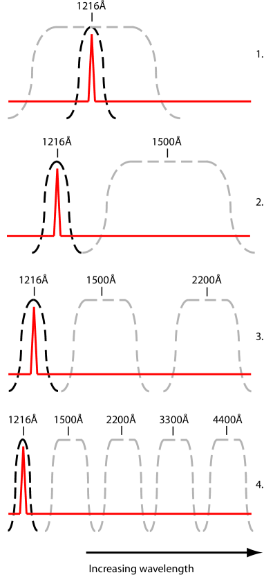
Figure 1: Schematic diagram of filter positioning for the four observational approaches described in Sect. 2.3 the text. Narrowband filters (on-line, black) have widths of 2% their central wavelengths and broadband filters (continuum, grey) have widths of 20% $\lambda_{\mathrm{c}}$. Wavelength indications represent central wavelength of the filters and are marked in the restframe of the SED. I.e. observation-frame filters are centred at $(1+z)\cdot\lambda_{\mathrm{c}}$. [See the electronic journal article for the colour version of this figure.]

The techniques are:

1. Narrowband on-line filter at redshifted Ly$\alpha$ and one broadband filter with the same central wavelength. While neither of these observations samples the line or continuum individually, they both sample the line-flux plus continuum; the flux in each filter is the sum of the line-flux ($F_{{\rm Ly}\alpha}$) and the product of the continuum flux-density ($f_{cont}$) and filter-width ($W$). If a flat continuum $(\beta=0)$ is assumed across the broadband filter, $F_{{\rm Ly}\alpha}$ and $f_{cont}$ can be obtained from the solution of two simultaneous equations as

   $$F_{line}=\frac{W_{\mathrm{b}}F_{\mathrm{n}}-W_{\mathrm{n}}F_{\mathrm{b}}}{W_{\mathrm{b}}-W_{\mathrm{n}}}\\ f_{cont}=\frac{F_{\mathrm{b}}-F_{\mathrm{n}}}{W_{\mathrm{b}}-W_{\mathrm{n}}}$$ (3)

   where $F$ and $W$ represent the flux and filter width, and subscripts $n$ and $b$ refer to the broad and narrowband filters, respectively. This is the same observational setup as used by Cowie & Hu (ref:cowiehu98 (1998)) and Fynbo et al. (ref:fynbo02 (2002)), and dividing the first part of Equ. 3 by the second, one obtains the equivalent width expression used by Malhotra & Rhoads (ref:malrhoads02 (2002)).

2. Narrowband on-line filter centred on redshifted Ly$\alpha$ and one completely off-line broadband filter centred at $(1+z)\cdot 1500$Å to sample the continuum. At 1500Å, a 20% (300Å full width) filter will not transmit the Ly$\alpha$ line itself. The continuum flux at Ly$\alpha$ can then be estimated by assuming the continuum can be approximated by a power-law of the form $f_{\mathrm{\lambda}}\propto\mathrm{\lambda}^{\beta}$, with arbitrary index $\beta$. This technique allows the investigation of the reliability of assuming the behaviour of the UV continuum slope in the situation where only one continuum observation is available.

3. Narrowband on-line filter centred at redshifted Ly$\alpha$ and two broadband continuum filters centred at $(1+z)\cdot 1500$ and $(1+z)\cdot 2200$Å. This method assumes the UV continuum can be approximated by a power-law of the same form as in technique #2. From the two continuum fluxes, the index $\beta$ is measured between restframe 1500Å and 2200Å. This $\beta$ is then used to scale the 1500Å flux to the domain sampled by the narrowband filter and estimate $f_{\mathrm{cont}}$ at 1216Å.

4. Narrowband on-line filter centred at redshifted Ly$\alpha$ and four broadband filters centred at restframe 1500Å, 2200Å, 3300Å, and 4400Å. These wavelengths are selected to correspond to the central wavelengths of the filters used in our HST/ACS imaging survey of local starbursts (Hayes et al. ref:hayes05 (2005)). In this study we found we could find non-degenerate fits in age – $E_{B-V}$ space if we sampled the UV continuum slope and 4000Å break. The same technique is adopted whereby we fit the synthetic SB99 spectra to the ‘real’ data. A standard least-squares algorithm is used for different ages and internal reddenings using a given reddening law. From the best-fitting synthetic spectrum, the flux ratio between the $(1+z)\cdot 1500$Å continuum filter and the narrowband on-line filter is computed. This scale-factor is then used to scale the observed continuum flux at 1500Å to the continuum flux in the spectral region sampled by the on-line filter.

3 The simulations

Our simulations aim to understand the way in which astrophysical conditions in the host-galaxy and inter-galactic medium (IGM) manifest themselves in the determination of $F_{{\rm Ly}\alpha}$ and $W_{{\rm Ly}\alpha}$. To this end, we devised a number of different tests, varying individually the parameters that describe the host galaxies, in order to examine their impact. In order to standardise the parameter setup, a ‘standard’ restframe template was defined, the key parameters of which can be seen in Tab. 1.

Table 1: The parameters of the ‘standard’ restframe SED

By default, single stellar populations are treated, with the inclusion of stellar and nebular emission, the relative contributions of which are left unchanged. Unless otherwise stated, the equivalent width of the Ly$\alpha$ line added to the spectrum is 100Å for ease of visualisation (I.e. fractional/percentage deviations are easily interpreted). No internal or Galactic extinction is applied to the spectra by default.

We determined it necessary to run tests to study the impact of redshift and H i absorption along the line-of-sight, internal dust reddening, and mixing of stellar populations. Burst age is not considered in this paper for the following reason: our preliminary tests showed that the recovery of $F_{{\rm Ly}\alpha}$ and $W_{{\rm Ly}\alpha}$ by all four techniques were self-consistent to within 2%, (no age dependence on the recovered observables with age) over the first 200Myr. In addition, Charlot & Fall (ref:cf93 (1993)) demonstrated Ly$\alpha$ in emission can only be expected from considerably younger star-forming galaxies of ages $\leq 40$Myr; over this time we found evolution in the observables below the 1% level.

Technique #2 allows for the UV continuum slope ($\beta$) to be arbitrarily chosen. In a large sample of LBGs re-sampled into quartiles according to $W_{{\rm Ly}\alpha}$, Shapley et al. (ref:shapley03 (2003)) find median values of $\beta=-1.09$ for the strongest Ly$\alpha$ emitters (upper quartile) with the continuum flattening to $\beta=-0.73$ for the weakest, lower quartile where the median $W_{{\rm Ly}\alpha}$ is -14.92Å. In contrast, the Starburst99 models show $\beta$ in the range -2.6 to -2.0 over the first $\sim 50$Myr. Excess flux in a narrowband filter $(n-b<X)$ is a typical selection function although the the amount of excess $X$ is arbitrarily chosen. $X=0$ would correspond to a flat continuum, whereas $X<0$ would imply the continuum level is rising towards Ly$\alpha$. While $X$ can be computed by making some simple assumptions, the range in the power-law index ($\beta$) from which $X$ would be computed can be very large. Without any additional data to constrain the continuum slope, any assumption is ad hoc but, for the sake of simplicity, in the simulations presented here we assume $\beta=0$ (i.e. a flat continuum). Moreover, only a modest dust content is required to flatten the steep continuum slopes observed in the FUV. Additionally, it should be mentioned that the Equ. 3 (technique #1) only holds exactly if $\beta=0$, although the total spectral region sampled by this technique is much smaller.

3.1 Cosmic distance and the IGM

Any two restframe SEDs generated from the same initial parameters are identical. The only way two identically created but redshifted SEDs can differ is via the differing effects that result from intervening H i in the IGM. The $z$-distribution and column density of H i clouds is pseudo-randomly generated, and as a result the redshifted SEDs can differ greatly. Thus a Monte-Carlo-type approach is adopted. A population of 10 000 restframe SEDs is generated which, after redshifting, differ only bluewards of Ly$\alpha$ (except for the possible red wing of DLA systems that may extend on to the red side of the line – the absorption line-centre is still on the blue side). For this population, mean and median averages of the fluxes and equivalent widths are then computed using the techniques described in Sect. 2.3. These computations are performed for populations at a range of redshifts between zero and $z=9.0$, the highest redshift at which narrowband survey techniques have been employed in an attempt to find LAEs (Willis & Courbin, ref:willis05 (2005)). In a real imaging survey, there must be additional selection criteria by which a candidate is determined to be an emitter. In this case, we also recompute these mean values after the rejection of all objects for which restframe $W_{{\rm Ly}\alpha}$ value was determined to be less than 20Å. This value is hereafter referred to as the “refined mean”.

It would also be interesting to simulate more realistic samples of galaxies. The Ly$\alpha$ luminosity function has been compiled at $z=5.7$ and 6.5 by Malhotra & Rhoads (ref:malrhoads04 (2004)). However, while spectroscopic observations were used in the compilation of these luminosity functions for statistical purposes, the luminosities of the LAEs themselves have been derived photometrically. Hence, they may well contain observational biases of the type we attempt to address here. Additionally, we would have to assume the characteristics of the observation itself such as sky-noise and it was deemed more revealing to study populations of identical objects.

3.2 Internal dust reddening

In the absence of intervening H i absorption, we study the effect of internal dust extinction on the reliability of our recovery of $F_{{\rm Ly}\alpha}$ and $W_{{\rm Ly}\alpha}$. Using the common starburst extinction laws [ Starburst: Calzetti et al. (ref:calzetti00 (2000)); SMC: Prévot et al. (ref:prevot84 (1985)); LMC: Fitzpatrick et al. (ref:fitz85 (1985)) ] we artificially redden the template SEDs and investigate how reliably the various techniques estimate Ly$\alpha$ and $W_{{\rm Ly}\alpha}$. Technique #4 relies upon fitting age and internal reddening in order to estimate the continuum flux at Ly$\alpha$. In these experiments, we also investigate the reliability of this technique when different extinction laws are used for the SED fitting from the one used to redden the intrinsic spectrum. This allows us to investigate how well Ly$\alpha$ observables are recovered if an inappropriate reddening law were assumed. For example, we redden the intrinsic SED with the SMC law and use the Calzetti law in the SED fitting routines. We then investigate whether possible improvements can be made by including the reddening law itself as a free parameter in the fitting routine. Tests are carried out in the range $0.0<E_{B-V}<0.5$ at redshifts of 2, 4, and 6.

3.3 Underlying stellar populations

Again without the effects of intervening H i systems, we investigate how accurately $F_{{\rm Ly}\alpha}$ and $W_{{\rm Ly}\alpha}$ are recovered when the Ly$\alpha$ emitting object hosts varying components from an underlying population. This is mainly relevant to technique #4 which relies upon sampling of the 4000Å break, and, while we don’t study $F_{{\rm Ly}\alpha}$ or $W_{{\rm Ly}\alpha}$ vs. age directly, this study addresses the effect an aged stellar population may have. As before we adopt the default template spectrum as a ‘primary’ SED (I.e. the single stellar population starburst spectrum defined in Tab. 1 with an age of 4Myr). We then add an assortment of older, post-starburst spectra to the primary, scaling to varying normalisation factors at a wavelength of 4500Å (i.e. scaling by the approximate $B-$band luminosity). We thereby artificially create young starburst galaxy spectra with a population of older stars. This normalisation factor is designated $n_{4500}$ and, by this definition: $n_{4500}=0$ is just the default SED defined in Tab. 1; $n_{4500}=1$ means the default and aged populations contribute equally at 4500Å; and $n_{4500}=10$ means the old population is a factor of 10 more luminous than the starburst SED at 4500Å. The parameters used in the generation of SED of the underlying population can be seen in Tab. 2 but briefly, we perform tests to examine the age of the underlying population, its metallicity, and its normalisation coefficient, $n_{4500}$. Then, after redshifting the SEDs, we investigate what values of $F_{{\rm Ly}\alpha}$ and $W_{{\rm Ly}\alpha}$ our techniques recover. When the SED-fitting technique is used (technique #4), we always used the unmodified set of starburst templates for fitting. Tests are performed at redshifts of 2, 4, and 6. Tab. 2 shows the different old stellar populations and their contributions as applied to the standard setup, along with the resulting $W_{{\rm Ly}\alpha}$ calculations.

4 Results and discussion

4.1 Cosmic distance and IGM

As described in Sect. 2.3 and Sect. 3.1 we generate populations of galaxies at a given redshift, and determine the mean, median, and refined mean values of observed $F_{{\rm Ly}\alpha}$ and $W_{{\rm Ly}\alpha}$ for this population using the four observational techniques. Fig. 2 shows a set of histograms representing the distribution of these observed quantities for a population of 10 000 galaxies at $z=5.7$, selected to correspond to the redshift of number of Ly$\alpha$ surveys (eg. Thommes et al. ref:thommes98 (1998); Rhoads & Malhotra ref:rhoads01 (2001); Westra et al. ref:westra05 (2005)). Restframe $W_{{\rm Ly}\alpha}$ is 100Å.

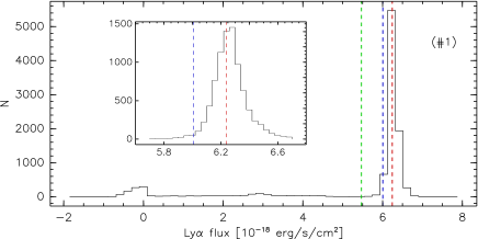
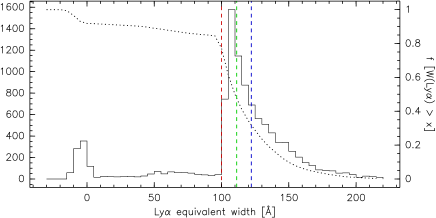
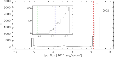
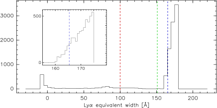
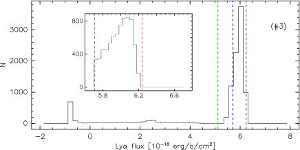
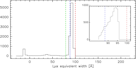
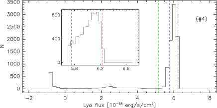
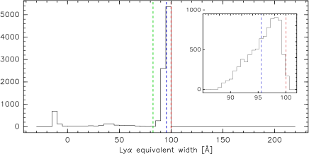
Figure 2: Histograms showing the distribution of detected Ly$\alpha$ flux (left) and equivalent width (right) for a population of 10 000 galaxies at a redshift of $z=5.7$. The descending pairs of plots represent distributions as computed by observational techniques #1, #2, #3, #4. The vertical dashed red lines indicate the true line flux and equivalent width (I.e. that added to the restframe SED). The vertical green line shows the mean values computed for the whole sample of 10 000 objects, while the blue line shows the mean value of these quantities for all objects with $W_{{\rm Ly}\alpha}$$>20$Å (refined mean). The dotted black line in the uppermost equivalent width plot shows the fraction of galaxies in the sample with observed $W_{{\rm Ly}\alpha}$ greater than the value on the abscissa axis (I.e. for that value of $W_{{\rm Ly}\alpha}$, the fraction of galaxies that have $W_{{\rm Ly}\alpha}$ greater than this value). [See the electronic journal article for the colour version of this figure.]

A noteworthy feature, present in all these plots is the population of $\sim 750$ galaxies with $F_{{\rm Ly}\alpha}$ and $W_{{\rm Ly}\alpha}$ around zero (and slightly negative). In the line-of-sight to these objects a DLA system has been generated near to the target LAE, the red damping wing of which has removed the Ly$\alpha$ line from the spectrum. The slight negativity of these values comes from the fact that, in order to estimate the line-only flux, the continuum has been subtracted and, in all these cases, continuum subtraction has resulted in negative fluxes in the line. These objects would not be found by imaging observations that target emitters and hence including them in the computation of average quantities would be misleading. This effect therefore leads to a redshift-dependent incompleteness, which at $z=6$ is about 10% for these filters. Such effects would need to be treated in the computation of the Ly$\alpha$ luminosity function. It is for this reason that we compute refined mean values for the population of objects with detected $W_{{\rm Ly}\alpha}$$>20$Å only.

Dashed vertical lines have been added to all these histograms in three colours. The red line shows the flux or equivalent width of the Ly$\alpha$ line that was added to the restframe spectrum, the green line shows the mean of the recovered quantities, and the blue line shows the refined mean.

The top pair of plots in Fig. 2 represent the quantities as determined using technique #1 (a narrow and broad filter centred at $(1+z)\cdot\lambda_{\mathrm{Ly}\alpha}$). The $F_{{\rm Ly}\alpha}$ histogram shows a strong peak in the distribution that perfectly corresponds to intrinsic line flux. The mean of the distribution falls 15% short of this value. The coincidence of the peak in flux distribution and intrinsic flux demonstrates the power of this method in determining line flux. The top right panel in this figure shows the distribution of $W_{{\rm Ly}\alpha}$ when computed by this technique (#1). While $F_{{\rm Ly}\alpha}$ is accurately recovered and evenly distributed around the correct value, the $W_{{\rm Ly}\alpha}$ distribution cuts on sharply at $W_{{\rm Ly}\alpha}$=100Å, peaks, and exhibits a long tail, extending to 220Å. While some flux may be removed from the narrowband filter by intervening H i clouds, the broadband filter samples the continuum significantly bluewards of Ly$\alpha$. Hence H i clouds in the IGM can remove a significant amount of flux from this broadband observation. Consequently, the continuum flux at Ly$\alpha$ can be drastically underestimated, resulting in a doubling of observed $W_{{\rm Ly}\alpha}$ in extreme cases. The black dotted line in this plot shows the fraction of objects with recovered $W_{{\rm Ly}\alpha}$ greater than the value on the abscissa. It crosses the red dashed line (100Å) at 0.8, implying that $W_{{\rm Ly}\alpha}$ has been overestimated for 80% of all the objects (including those with $W_{{\rm Ly}\alpha}$$\sim 0$ that represent the incompleteness in the observed population). After removing the $W_{{\rm Ly}\alpha}$$\sim 0$Å objects, this fraction is more like 90%.

The second pair of plots represents the distribution of the same detection properties, as determined by technique #2. Here the same on-line filter is used but a single broadband filter centred at $(1+z)\cdot 1500$Å is used to estimate the continuum at Ly$\alpha$ by assuming $\beta=0$ between the spectral regions sampled by these filters. Since our standard restframe template is that of a 4Myr starburst with no dust, the continuum is increasing towards the line ($\beta\sim-2.6$) and the subtraction of an underestimated continuum results in a slight shift of the distribution towards higher fluxes. In this case where the line is strong, the measured flux in the narrowband filter is dominated by the line, and the relative effect of underestimating the continuum is small. We have verified that the effect is more significant when smaller rest equivalent widths are input (i.e. continuum-dominated observations). In this example, underestimating the continuum flux has a more pronounced impact upon the estimate of $W_{{\rm Ly}\alpha}$ and the mode in the $W_{{\rm Ly}\alpha}$ distribution is shifted from 100Å to $\sim 170$Å. While technique #2 may provide reliable line-fluxes when the line is strong, any equivalent widths derived in this manner cannot be considered robust. Even if there is no line ($W_{{\rm Ly}\alpha}$$=0$), for a young, unreddened burst with $\beta<0$, the assumption of $\beta=0$ will result in a positive observed equivalent width and false positive detection of narrowband excess.

Techniques #3 and #4 reliably reproduce both $F_{{\rm Ly}\alpha}$ and $W_{{\rm Ly}\alpha}$ in this study. Technique #3 assumes the UV continuum slope to be a power-law between 2200Å and Ly$\alpha$ and uses off-line filters placed at restframe 1500 and 2200Å to extrapolate to Ly$\alpha$. Technique #4 makes no assumptions about the continuum, and uses a 4-filter SED-fitting technique to estimate the continuum level at Ly$\alpha$. With the exception of the small peaks around $F_{{\rm Ly}\alpha}$ and $W_{{\rm Ly}\alpha}$=0, these distributions are strongly peaked around their intrinsic values. The narrow distribution of $W_{{\rm Ly}\alpha}$ demonstrates how successful these techniques are at estimating the continuum fluxes at line-centre. The refined mean values of $W_{{\rm Ly}\alpha}$ are in error by only $\sim 5$%.

In reality, all the accuracy of all these results would be dependent on the recovered flux in the various bands and the sky-noise. While this is not strictly the angle we have chosen for this article, we investigate and discuss the effects of sky noise below. Fig. 4 demonstrates how the various technique fare near the detection limit with the the application of a simple sky-noise model.

Fig. 3 shows the evolution of the total mean, refined mean, and median values of $F_{{\rm Ly}\alpha}$ and $W_{{\rm Ly}\alpha}$ as a function of redshift. The blue curves represent technique #1, green curves technique #2, red curves technique #3, and black curves technique #4. The flux values are the average observed fluxes, normalised by the computed intrinsic line flux at the observatory (i.e. the intrinsic line-luminosity scaled down by the luminosity distance).

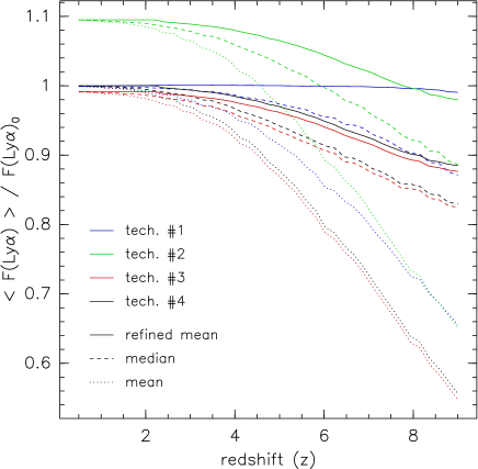
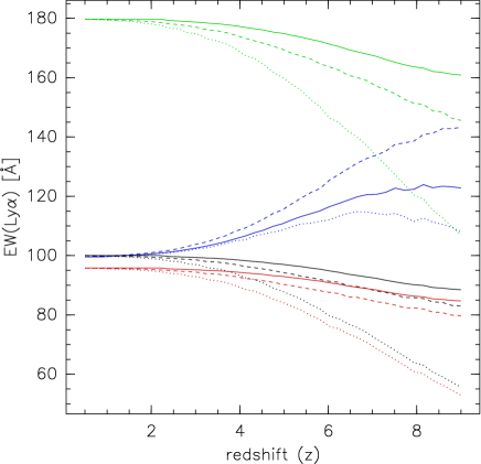
Figure 3: The evolution of $F_{{\rm Ly}\alpha}$ and $W_{{\rm Ly}\alpha}$ as function of redshift. The left plot shows the recovered $F_{{\rm Ly}\alpha}$, normalised by the predicted flux at the observatory, calculated from the intrinsic line luminosity added in the restframe (I.e. the fractional deviation from the true value). The right plot shows the evolution of $W_{{\rm Ly}\alpha}$. Colour blue represents technique #1, green: technique #2, red: technique #3 and black: technique #4. Dotted lines represent total mean values, dashed lines represent median values, and solid lines show the refined means. [See the electronic journal article for the colour version of this figure.]

As previously discussed, technique #1 reliably recovers $F_{{\rm Ly}\alpha}$ in the line-dominated limit and this is here demonstrated to be independent of redshift. However, $W_{{\rm Ly}\alpha}$ as computed using this technique becomes progressively worse with increasing redshift as can be seen from the right plot – the refined mean value for $W_{{\rm Ly}\alpha}$ at $z=6.5$ is overestimated by 20%. This is a result of the increasing redshift-density of intervening clouds with redshift $(\propto(1+z)^{2.45})$, causing a systematic decrease of the estimate of the continuum flux. Technique #2 overestimates $F_{{\rm Ly}\alpha}$ by $\sim 10$% at $z=2$. This results from the assumption of a flat spectrum not accounting for the blue continuum slope of a young stellar population. This technique is unreliable in estimating $W_{{\rm Ly}\alpha}$ and at all redshifts as the right plot shows, never comes close to estimating the correct $W_{{\rm Ly}\alpha}$. Again as demonstrated in Fig. 2, techniques #3 and #4 both reliably determine $F_{{\rm Ly}\alpha}$ and $W_{{\rm Ly}\alpha}$ at low and high redshift – the refined mean values of $W_{{\rm Ly}\alpha}$ deviate from the expected values by less than 9, and 5%, respectively, at $z=6$.

It is, of course, possible to fit a function to any of the redshift-evolution curves shown in Fig. 3, thus obtaining a functional prescription for the fractional under- or over-estimate of $F_{{\rm Ly}\alpha}$ and $W_{{\rm Ly}\alpha}$ as a function of redshift. Such a formula would be highly desirable as it would be directly applicable to the results obtained by previous surveys. However such a corrective formula would not only be a function of redshift, but also of the filter widths, response profiles, and positioning in wavelength. Of course, such information is well-known and we recommend simulations to be carried out on a survey-by-survey basis, and with appropriate consideration of the errors and selection criteria.

Malhotra & Rhoads (ref:malrhoads02 (2002)) used a technique similar to technique #1 to observe LAEs at a redshift of 4.5, uncovering a population of galaxies with curiously high equivalent width (median $W_{{\rm Ly}\alpha}$$\sim 400$Å). Since there is no AGN activity associated with these objects (Wang et al. ref:wang04 (2004)) and the maximum $W_{{\rm Ly}\alpha}$ available from star-formation (with ‘normal’ IMFs and metallicities) is 240Å (Charlot & Fall ref:cf93 (1993)), such a discovery attracts speculation. Using our simulations we determine that at $z=4.5$, the median value of $W_{{\rm Ly}\alpha}$ may be overestimated by a factor of only $\sim 12$% – clearly Malhotra & Rhoads’ high-$W_{{\rm Ly}\alpha}$ result is not an observational effect of the type under consideration in this article. However, the effect of intervening H i on $W_{{\rm Ly}\alpha}$ as computed by technique #1 is that a large spread in $W_{{\rm Ly}\alpha}$ is produced (see Fig. 2, top right), leading to a significant fraction of LAEs with overestimated $W_{{\rm Ly}\alpha}$ – 20% of all the objects have $W_{{\rm Ly}\alpha}$ overestimated by more than 40%. Certain selection functions (eg. narrowband excess) will then be more inclined to pick up these objects.

In order to further investigate some more realistic observational effects, we implemented a simple noise model. Taking the fluxes obtained from the population of objects shown in Fig. 2 (10 000 objects at $z=5.7$ with $W_{{\rm Ly}\alpha}$=100Å), we assumed that the criterion for a ‘detection’ is $5\sigma$. We then assigned a $S/N=5$ to each narrowband flux, and weighted this by the ratio of detected $F_{{\rm Ly}\alpha}$ to the intrinsic line flux ($F_{\mathrm{Ly\alpha,0}}$). $S/N$ was assigned to the broadband observations in an identical manner: 5 weighted by the ratio of the observed flux to the intrinsic flux. Note this weighting modification of $S/N=5$ is only applicable to the broadband filter centred at Ly$\alpha$ – the redder filters are not affected by H i clouds in the IGM, and all have $S/N=5$. With $\sigma$ for all the observations, we used Box-Muller transforms to generate Gaussian deviates around the fluxes in each passband. We fed these fluxes back into the expressions used to derive $W_{{\rm Ly}\alpha}$ and replotted the resulting distributions of $W_{{\rm Ly}\alpha}$ which can be seen in Fig. 4.

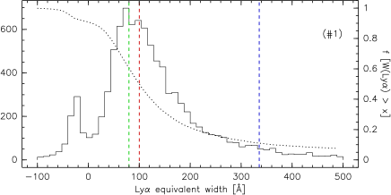
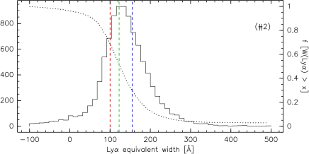
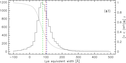
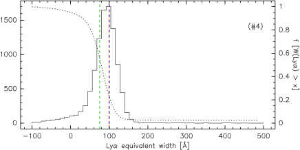
Figure 4: Histogram showing the detected $W_{{\rm Ly}\alpha}$ of 10 000 galaxies at $z=5.7$. These are the same objects as plotted in Fig. 2 but fluxes have been regenerated within assumed observational errors from a simple assumed noise model. Dotted line and vertical dashed lines as in Fig. 2. [See the electronic journal article for the colour version of this figure.]

In all cases, the main distribution is now significantly broadened; the mode has shifted towards lower values of $W_{{\rm Ly}\alpha}$, and a high $W_{{\rm Ly}\alpha}$ tail has been produced. This results from the fact that equivalent width is the quotient of two values $(F_{\mathrm{Ly\alpha}}/f_{cont})$. Symmetrical redistribution of the denominator results in asymmetric redistribution of the combined quotient; compressed on the low side of the mean (lowering the mode) and extended at high values. This is most striking using technique #1 since signal in the broad filter is lost to H i absorption in the IGM – $\sim 20$% of objects have $W_{{\rm Ly}\alpha}$ overestimated by a factor of 2. Still the number of objects scattered to very high $W_{{\rm Ly}\alpha}$ is small overall, we reiterate that some selection criteria will include them: in a narrowband survey they are likely to exhibit clear narrowband excess. Redistribution of Ly$\alpha$ has caused the plots for all techniques to appear similar: modes have been reduced slightly and extended, high-$W_{{\rm Ly}\alpha}$ tails are present. One noteworthy feature about the progression from technique #1 through #4 is the movement of the refined mean of the distribution (blue vertical line) towards the intrinsic value of 100Å, and for the same reason, the steepening of the black dotted line. The addition of more filters is necessary to prevent the extreme spreading of the distribution and scattering to extreme values of $W_{{\rm Ly}\alpha}$. For technique #4 the refined mean value now accurately recovers the intrinsic values of $W_{{\rm Ly}\alpha}$, and $W_{{\rm Ly}\alpha}$ is overestimated by more than 50% for very few objects.

4.2 Internal dust

The tests presented here showed indistinguishable results at redshifts of 2, 4, and 6, hence the results we present regarding reddening can be assumed to be independent of redshift. Fig. 5 shows how well $W_{{\rm Ly}\alpha}$ is recovered for some test cases when dust is added to the system. The internal reddening for a given extinction law (type of dust) is represented on the abscissa of the plots, while the recovered value of $W_{{\rm Ly}\alpha}$ is presented on the ordinate. Where the SED-fitting technique (#4) is concerned, the assumed extinction law used by the SED-fitting routine may be different from that used to redden the restframe SED and can be seen in the central caption of each figure. In the tests presented here we only redden the restframe SEDs using the Calzetti and SMC laws because all other laws show a 2175Å graphite feature. If we believe we are dealing with objects with a very strong UV radiation field, larger graphite-based molecules will be destroyed, removing any 2175Å feature from the reddening vector and producing a law similar to that of the SMC (Mas-Hesse & Kunth ref:mhkunth99 (1999)). We now only consider the impact upon the determination of $W_{{\rm Ly}\alpha}$, having shown it to be a much more sensitive performance indicator than $F_{{\rm Ly}\alpha}$. Intervening H i absorbing systems have been “switched off” for this experiment. The range in $0.0<E_{B-V}<0.5$ is chosen.

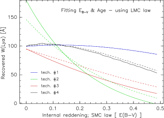
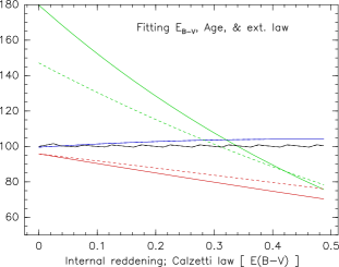
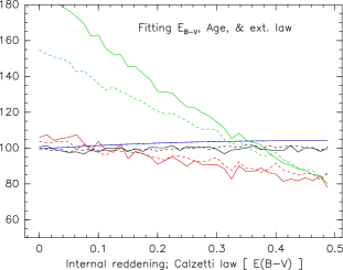
Figure 5: Recovered $W_{{\rm Ly}\alpha}$ as a function of internal reddening using the starburst extinction laws. The abscissa shows the internal reddening $E_{B-V}$, using a known extinction law. The ordinate shows the recovered value of $W_{{\rm Ly}\alpha}$ using an an extinction law assumed by the observer. Left: True dust: SMC-law; assumed dust: LMC. Centre: True dust: Calzetti-law; extinction law free parameter in SED fitting routine Right: As for centre but with noise model applied. Colours represent observational strategies as in Fig. 3. The filter setup is as described in section 2.3 (solid lines). The dashed lines show the same results but with the nearest off-line filter (restframe 1500Å) shifted to 1400Å. [See the electronic journal article for the colour version of this figure.]

Technique #1 (blue line) is here demonstrated to very accurately recover $W_{{\rm Ly}\alpha}$ in all cases shown. At $E_{B-V}=0.5$ this technique overestimates $W_{{\rm Ly}\alpha}$ by just 3% using the Calzetti law (central panel) and the technique is largely insensitive to dust. This minor effect is a result of the steepening extinction curve removing flux from the broad bandpass, leading to a mild overestimate of the continuum flux at Ly$\alpha$. Conversely, this technique underestimates $W_{{\rm Ly}\alpha}$ by 13% for SMC-type dust (left panel). Across the wavelength range of the 1216Å-centred broad bandpass $(\sim 1000\AA$ to $\sim 1340\AA)$, the SMC-law provides more extinction than the Calzetti law for a given $E_{B-V}$, and has a steeper gradient (more rapidly increasing with decreasing wavelength). This results in the stronger suppression of the Ly$\alpha$ line with the SMC law than that of Calzetti, and turns the mild overestimate of $W_{{\rm Ly}\alpha}$ into a more significant underestimate.

Technique #2 (green lines) is highly ineffectual at reproducing the intrinsic equivalent width when dust is added to the system. This is also dependent upon the chosen extinction law: SMC-type dust (left panel) completely suppresses the unreddened excess of a $W_{{\rm Ly}\alpha}$$=100$Å line relative to the 1500Å flux by $E_{B-V}=0.48$. That is, using technique #2, at $E_{B-V}>0.48$ an LAE of $W_{{\rm Ly}\alpha}$$=100$Å will be seen as a Ly$\alpha$ absorber. This effect is nowhere near as extreme when the Calzetti law is applied since the SMC law is significantly steeper in the FUV.

Modeling the UV continuum ($\beta$) as a simple power-law (technique #3; red lines) and extrapolating to Ly$\alpha$ only performs marginally better in the presence of dust. A clear downward trend is visible with $E_{B-V}$, although the dependency is highly sensitive to the extinction law. At the relatively modest value of $E_{B-V}=0.1$, a Ly$\alpha$ emitting object will have $W_{{\rm Ly}\alpha}$ underestimated by around 10% using the Calzetti law but by 25% for SMC dust. By $E_{B-V}=0.5$ using the Calzetti law, $W_{{\rm Ly}\alpha}$ is underestimated 30%, while for SMC dust the line has been almost completely suppressed. Extrapolating $\beta$ does not provide a reliable estimate of $W_{{\rm Ly}\alpha}$ when even a modest amount of dust is present since the dust extinction curve modifies $\beta$ in such a way that it becomes inconsistent with a power-law approximation. The dashed lines in Fig. 5 show how recovery of $W_{{\rm Ly}\alpha}$ is only very slightly improved when the continuum filter sampling 1500Å is moved to 1400Å. Of course, it stands to reason that moving the off-line filter nearer to the line is going to yield a better result and this is something that must be considered when designing any observation – even when the filters can be ideally placed (which is also subject to the presence of sky lines), the gain may not be significant.

Clearly technique #1 is not greatly susceptible to the effects of internal dust reddening. In contrast, techniques #2 and #3 are highly susceptible to dust and these observational configurations do not provide enough information to handle any reddening in a reliable manner. Continuum extrapolation techniques are not sufficient and a technique is required that either handles the reddening explicitly or covers a sufficiently narrow spectral domain. Indeed, the technique #4 also becomes increasingly unreliable with increasing dust content if the extinction law/dust type is not well known – assuming the wrong dust type renders the SED fitting method ineffective (Fig 5, left panel). However, the 2200Å continuum filter is well positioned to sample the 2175Å graphite feature in the reddening vector. This enables a third dimension to be added to the SED-fitting routine: the discrete parameter of the dust extinction law. By fitting age, extinction law, and $E_{B-V}$, we are able to recover $W_{{\rm Ly}\alpha}$ to within 1% for all values of $E_{B-V}$ for each of the extinction laws. See the central panel of Fig. 5 for and example using Calzetti law.

Due to concerns about fitting three parameters with noisy data, we adopted a similar noise-model to that described in Sect. 4.1. Of particular concern was whether we could accurately recover the extinction law. All fluxes were assigned $S/N=5$, randomised within the corresponding Gaussian $\sigma$, and plugged back into the formulae to compute $W_{{\rm Ly}\alpha}$. We now generate 1 000 LAEs for each point in $E_{B-V}$, and compute the mean values recovered. Since there are no H i IGM clouds in this simulation, there is no non-recovered population to that needs to be taken into consideration. The results can be seen in the right panel of Fig. 5. Clearly, at the $5\sigma$ limit, the concerns about recovery of the reliability of the fitting routine are not serious – the SED fitting routing recovers $W_{{\rm Ly}\alpha}$ to within 3% in all cases.

Obtaining such observations of continuum-faint objects at high-$z$ requires a substantial investment of time; many narrowband Ly$\alpha$ surveys find a significant population of objects with no apparent UV or optical continuum. This is one of the areas in which the class of extremely large optical telescopes has the opportunity to make a significant impact: with gains in collecting area of a factor of 25, restframe UV detections of dusty systems may become more of a possibility. This is one of the reasons why we push this study to seemingly extreme values of $E_{B-V}$. If detections can be made, this will be of importance given that many Ly$\alpha$ blobs (LABs) have been detected by narrowband imaging observations. A significant fraction of these LABs are also bright sub-mm sources (Chapman et al. ref:champman05 (2005); Geach et al. ref:geach05 (2005)) implying a very significant dust content and therefore reddening of the stellar continuum, although it has not been demonstrated that the Ly$\alpha$ and sub-mm radiation originate from the same regions of the galaxy. This is particularly true if the Ly$\alpha$ production in LABs is the result of accretion of cold gas onto dark matter halos (eg. Haiman et al. ref:haiman00 (2000)) in which case the Ly$\alpha$ may be emitted over significantly extended areas. There may also be a certain degree of decoupling between Ly$\alpha$ photons and the nearby UV continuum due to resonance scattering. In the cases where there is no continuum detection at all in any bands, (eg. Nilsson et al. ref:nilsson06 (2006)) then equivalent width has no meaning. However, if there is a detection of (potentially reddened) stellar continuum then total SED will be the superposition of this with the gas spectrum that gives rise to Ly$\alpha$, whatever the mechanism for its production. In this case, the SED fitting approach should be applicable and Ly$\alpha$ equivalent widths should be recoverable.

4.3 Underlying stellar populations

Again intervening H i absorbing systems have been switched off for these experiments and we only consider the Ly$\alpha$ equivalent width. Tests here are carried out using the standard template spectrum (defined in Sect. 3, Tab. 1) combined with various old stellar populations at redshifts of 2, 4, and 6. However, within the tests performed here, no redshift dependence at all was detected and hence, none will be discussed. The results presented here can be considered to hold at all redshifts.

Tab. 2 shows the way in which varying the contribution from an old stellar population affects the computed values of $W_{{\rm Ly}\alpha}$ when the age and metallicity of the underlying population are varied. Fig. 6 demonstrates the effect of increasing the relative contribution of a 300Myr underlying population.

Table 2: The influence of old stellar populations on detected $W_{{\rm Ly}\alpha}$ – the effects of age and metallicity.

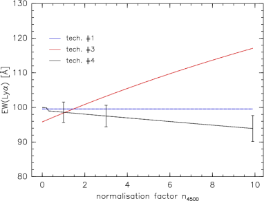
Figure 6: The effect of varying $n_{4500}$ on the recovered values of $W_{{\rm Ly}\alpha}$ as determined by the various techniques. $n_{4500}$ is defined in Sect. 3.3. The error bars on the black line show the standard deviation in recovered $W_{{\rm Ly}\alpha}$ when 1 000 objects are generated using the noise model described in the text. [See the electronic journal article for the colour version of this figure.]

For the tests presented for the age and metallicity of the underlying population, $n_{4500}$ is set to 1 in every case, meaning the underlying population and starburst SEDs contribute equally in the $B$-band. Clearly technique #1 is entirely unaffected by the presence of an aged stellar population, being in error by no more than 0.5% in every case. Again, the strength of this technique results from the fact it is dependent only on a very narrow spectral region. Technique #2 is consistently inaccurate, showing the typical overestimate of $W_{{\rm Ly}\alpha}$ by $\sim 70$% but is self-consistent to within about 10%. Technique #3 is accurate to within 10%. The 4-filter SED-fitting technique (#4) implemented here is included in this study because we have demonstrated it to be a reliable technique by which the continuum at Ly$\alpha$ can be accurately estimated (Hayes et al. ref:hayes05 (2005)). The strength of this technique relies on the UV continuum slope and 4000Å break being adequately sampled: then the effects of age and reddening aren’t completely degenerate and can be disentangled. Naturally, if the 4000Å break is so important, it is possible that the presence of an additional stellar population that contributes strongly to the 4000Å break but not in the UV could render this technique ineffective. No real trend of $W_{{\rm Ly}\alpha}$ with metallicity is observed with any of the techniques. A trend of $W_{{\rm Ly}\alpha}$ with the age of the underlying stellar population does emerge when computed using techniques #2, #3, and #4: recovered $W_{{\rm Ly}\alpha}$ decreases as the underlying population gets younger. The populations are normalised in the restframe at 4500Å but the SEDs become bluer with decreasing age. Hence, applying a younger underlying population has the effect of making the composite SED bluer than when an older population is added. As a result, the younger the underlying population, the higher the flux at 1500Å which leads to a tendency to overestimate the continuum at Ly$\alpha$. Therefore the estimates of the continuum level at Ly$\alpha$ become higher and the computed equivalent width is decreased.

When considering dependencies upon the normalisation coefficient, no trends emerge when using technique #1, (for the same reasons this technique is not sensitive to the age of the underlying population; Fig. 6). Technique #3, which extrapolates the measured value of $\beta$ to Ly$\alpha$, tends to overestimate $W_{{\rm Ly}\alpha}$ with increasing $n_{4500}$. As $n_{4500}$ increases, the flatter SED of the old population has the effect of flattening in the spectrum in the 1500-2200Å region. However, the 300Myr burst turns over towards Ly$\alpha$ much more sharply than the very young SED, and hence doesn’t contributed much at 1216Å. Hence the continuum flux at Ly$\alpha$ is increasingly underestimated as $n_{4500}$ increases. There is a minor tendency for technique #4 to become less accurate with increasing $n_{4500}$, underestimating $W_{{\rm Ly}\alpha}$ by 6% at $n_{4500}=10$. The fitting software selects increasingly older template spectra as the old population contributes more and more to the 4000Å break. However, with increasing $n_{4500}$, the composite spectrum changes faster across the 4000Å break than it does in the FUV. So as older (redder intrinsically) spectra are selected by the fitting software, in order to maintain a good fit in the UV, the best-fit SED will be less reddened than it would otherwise. This leads to a tendency to slightly overestimate the continuum flux at Ly$\alpha$, and a trend of underestimating $W_{{\rm Ly}\alpha}$ with increasing contribution from an older population.

In light of these results we made a number of attempts to confuse our SED-fitting software. The first was to, as in previous sections, see how the SED fitting routine fared when the simple noise model was applied. After applying the aged population at each value of $n_{4500}$, we randomised all the computed fluxes by assigning $S/N=5$ in each filter, and computed $W_{{\rm Ly}\alpha}$ from these values. We generated 1 000 objects and computed the mean values although these were never found to be deviant from the values computed without the noise model at all $n_{4500}$. The standard deviation of the recovered $W_{{\rm Ly}\alpha}$is represented by the error-bars on the black line (technique #4) of Fig. 6.

Secondly, we randomly selected old populations from any of the templates with ages greater than 300Myr, reddened them with random $E_{B-V}$ in the range 0.0 – 1.0, and added them to the template SED with varying $n_{4500}$ (range: 0.0 – 3.0). By applying two old populations to our template spectra in this fashion, we were not able to make technique #4 reproduce $W_{{\rm Ly}\alpha}$ that was in error by more than 10%.

The final test devised to confuse the software was to vary the contribution of the nebular continuum in the template spectra. The motivation for this test again being that the SED-fitting software is sensitive to the Balmer jump. Moreover, our understanding of the ionising photon production from massive stars is incomplete. There is a lack of data concerning low-metallicity stars, no single O type stars can be observed at such FUV wavelengths, and the ionising contribution from population iii objects is largely speculative. Additionally, Lyman-continuum escape has been observed in very few cases: Bergvall et al. (ref:bergvall06 (2006)) at low-$z$ in the case of ESO 350-IG38; and Steidel et al. (ref:steidel01 (2001)) at high-$z$ by stacking composite spectra of Lyman Break Galaxies (LBGs). It is the reprocessing of these photons that determines the intensity of the nebular component relative to that of the stars, hence any Lyman continuum photons that escape are not reprocessed in the nebular hydrogen emission spectrum (lines or continuum). We found that, even when scaling the nebular component (see Sect. 2.1) by a factors in the range $0-3$, technique #4 recovered $W_{{\rm Ly}\alpha}$ with errors no greater than 5%. These limits extend between two very extreme cases: one, where all Lyman continuum photons escape (which would result in no nebular emission component and therefore no Ly$\alpha$); and two, the possibility that the estimates of ionising continuum in stellar atmosphere models are in error by a factor of 3 and all the ionising photons are reprocessed as nebular emission.

4.4 Redshift and observational dependencies

One of the initial motivating factors for the study of Ly$\alpha$, dating back to Partridge & Peebles (ref:pp67 (1967)), was the fact that it could provide a tracer of early star formation observable from the ground at redshifts greater than around 2. At $z=2$, technique #1 would be equivalent to a narrowband filter at 3600Å, plus a $U$ filter. Here the effect of intervening H i systems will be lower than at higher $z$ and, at the lowest redshifts where Ly$\alpha$ is observable from the ground, intervening H i affects the determination of $W_{{\rm Ly}\alpha}$ by technique #1 at the 1% level for our chosen filter set. That said, any single measurement by this technique cannot be deemed reliable without additional observations. Followup spectroscopy could obviously confirm the presence of intervening systems and would also yield an accurate measurement of $W_{{\rm Ly}\alpha}$, but observational requirements may preclude the possibility of obtaining such data for every target. Perhaps cheaper, depending on the design of the survey, would be to use two off-line filters, say $B$ and $V$ (restframe 1470Å and 1830Å, respectively – where CCDs are typically more sensitive than in $U$), in order to estimate the continuum level at Ly$\alpha$ without sampling bluewards of 1216Å. However, the Shapley et al. (ref:shapley03 (2003)) LBG sample find median $E_{B-V}$ of 0.099 for the strongest Ly$\alpha$ emitters with $E_{B-V}$ increasing with decreasing $W_{{\rm Ly}\alpha}$. At $E_{B-V}=0.1$, technique #3 is already underestimating $W_{{\rm Ly}\alpha}$ by 25% for SMC dust. The dust-sensitivity of technique #3 is independent of redshift and will not be discussed further. At $z=2$, the 4000Å break can still be sampled by an observation in the $J-$band allowing technique #4 to be used in order to properly handle the effects of dust reddening.

As redshift increases, the effect of intervening H i on technique #1 becomes more pronounced, reaching the 10% level by $z=4$. Systematic uncertainties on numbers derived by this technique only should probably be addressed using a Monte Carlo-type approach. At this redshift, the 4000Å break can still be sampled from the ground using the $K_{\mathrm{s}}$ band although the high night-sky background makes these observations expensive. In 40 hours of integration time on an 8 metre telescope, a typical $K_{\mathrm{s}}-$band imaging camera can detect an object of $K_{\mathrm{s}}=24$ in the $AB$ magnitude system at $S/N=5$ . At $z=4$, and assuming the local $B-$band luminosity function (Jones et al. ref:jones06 (2006)) evolves parallel to the LF at 1500Å between redshifts of 0, (Wyder et al. ref:wyder05 (2005)) and 4 (Yoshida et al. ref:yoshida06 (2006)), this corresponds to a detection limit 0.5 mag fainter than $M^{\star}$. According to James Webb Space Telescope (JWST) Mission Simulator and NIRCam sensitivity estimates, such observations to these depths can be obtained at $2\mu m$ in just 1 second.

At redshifts greater than 5, $L-$band observations would be required in order to sample the 4000Å break. While deep observations may be obtainable from the ground at shorter wavelengths, the sky-background at wavelengths longer than $K_{\mathrm{s}}$ preclude such observations and current groundbased facilities do not approach the required sensitivities. Consequently these observations would need to be carried out by mid-infrared telescopes in more unfriendly and expensive environments: for example the Spitzer Space Telescope or JWST, or a proposed MIR telescope at Dome-C, Antarctica. This is somewhat contrary to the motivation for using Ly$\alpha$ as a probe for primeval star-formation. However, we reiterate that it is only this observation that needs to be done from space – the other bands may, depending on redshift, more economically be performed from the ground. Moreover, in the age of deep multi-band surveys, the amount of pre-existing data there is for a field is always a consideration. If observing a deep field at a certain wavelength, it may well be advantageous to select fields for which much data is already in existence – observations at new wavelengths are frequently added to existing datasets (the Chandra Deep Field, for example). Hence the majority of the observations required for technique #4 (targeting certain redshifts, at least) may already be in place, requiring only the additional infrared bands and it would be wise for future Ly$\alpha$ surveys to capitalise on the currently existing data. It is also likely that early JWST programs will include deep observations of regions with existing deep optical data.

In addition to the observational, there are also further theoretical uncertainties; mainly concerning the validity of the stellar atmosphere models in the UV. These models have currently not been well tested at these wavelengths. See Sect. 4.3 for a discussion on this.

5 Conclusions and summary

Simulations of observations of high-redshift Ly$\alpha$ emitting galaxies have been performed. Specifically, the simulations have examined how efficiently the intrinsic values of Ly$\alpha$ flux and equivalent width are recovered by narrowband imaging observations. $F_{{\rm Ly}\alpha}$ and $W_{{\rm Ly}\alpha}$ are determined by the four methods described in Sect. 3 and the effects of intervening H i clouds, internal dust-reddening, and underlying stellar populations, have been investigated. In summary:
– Observing Ly$\alpha$ with one off-line continuum filter has been shown to be highly ineffectual. The steep UV continuum slope ($\beta$) may cause overestimates of $W_{{\rm Ly}\alpha}$ by a factor of almost 2, while the neglection of dust reddening may cause the reverse effect: narrowband imaging observations may interpret bright Ly$\alpha$ emitters ($W_{{\rm Ly}\alpha}$$>100$Å) as Ly$\alpha$ absorbing systems.
– Using two filters to estimate the UV continuum slope and extrapolating to Ly$\alpha$ using a power-law improves the situation to varying degrees. In the dust-free cases this technique becomes a highly competitive method of determining $F_{{\rm Ly}\alpha}$ and $W_{{\rm Ly}\alpha}$. However, even modest amounts of dust render this technique highly ineffectual since dust modifies the continuum in such a way that the power-law parameterisation becomes unreliable. $E_{B-V}=0.1$ results in 25% underestimate of $W_{{\rm Ly}\alpha}$.
– Economic observing strategies that utilise a narrowband and single broadband filter with the same central wavelength are far less susceptible to dust. However, the continuum flux estimation in such observations becomes suspect due to the blue half of the broadband filter being on the blue side of Ly$\alpha$, and hence being susceptible to absorption of the continuum by intervening H i clouds. Such a technique can lead to overestimates of $W_{{\rm Ly}\alpha}$ by factors of $>2$. With the addition of a simple sky-noise model, this effect becomes more pronounced with decreasing $S/N$. We suggest that in such observations, simulations are performed to estimate the biases caused by such effects.
– SED-fitting techniques that observe only redwards of Ly$\alpha$ are not susceptible to intervening H i absorption or dust reddening, when a single extinction law is considered at all wavelengths. Such techniques need to sample the UV continuum slope, 2175Å dust feature, and 4000Å break. This way reliable estimates of the continuum flux at Ly$\alpha$ can be made and $W_{{\rm Ly}\alpha}$ estimates are much better constrained in the presence of noise.
– None of the techniques we considered here were hugely sensitive to the presence of underlying old stellar populations or randomly mixed populations. Additional populations have no detrimental effect on the efficiency of the technique utilising two filters centred on Ly$\alpha$. The contribution of such populations to the 4000Å break cause only minor ($<10$%) errors in the SED-fitting routine. Similarly increasing the relative contribution of nebular emission has no significant impact upon the estimates of $F_{{\rm Ly}\alpha}$ and $W_{{\rm Ly}\alpha}$.
– Independent of technique, we find a redshift-dependent incompleteness that results from H i systems along the line-of-sight. Such an effect would have to be allowed for in the compilation of a Ly$\alpha$ luminostiy function. The red damping wing of DLAs close to the LAE can remove sufficient flux to completely suppress the Ly$\alpha$ line. At $z=6$, one could expect to miss around 10% of the sources using our perfect filter set.

We have shown that to recover $F_{{\rm Ly}\alpha}$ and $W_{{\rm Ly}\alpha}$ from high-$z$ LAE systems, a SED fitting method is preferable if observations can reach the required depths. Other techniques suffer badly from either Ly$\alpha$ absorption along the line-of-sight or reddening by internal dust. If such off-band observations are not available, the use of a single narrow- and broadband filter with the same central wavelength seems to be preferable, although such observations should be complemented with some tuned statistical study of the effects of intervening H i systems.

- (1) Bergvall, N., Zackrisson, E., Andersson, B.-G., et al., 2006, A&A, 448, 513
- (2) Calzetti, D., & Kinney, A. L., 1992, ApJ, 399, L39
- (3) Calzetti, D., Armus, L., Bohlin, R. C., et al., 2000, ApJ, 533, 682C
- (4) Cardelli, J. A., Clayton, G. C., & Mathis, J. S., 1989, ApJ, 345, 245
- (5) Chapman, S. C., Blain, A. W., Smail, I., Ivison, R. J., 2005 ApJ, 622, 772C
- (6) Charlot, S., & Fall, S. M. 1993, ApJ, 415, 580
- (7) Cowie, L. L., & Hu, E. M. 1998, AJ, 115, 1319
- (8) Crowther, P., Prinja, R., Pettini, M., Steidel, C., 2006, MNRAS, 368, 895
- (9) Ellison, S. L., Hall, P. B., & Lira, P. 2005, AJ, 130, 1345E
- (10) Fitzpatrick, E. L. 1985, ApJ, 299, 219
- (11) Fynbo, J. P. U., Ledoux, C., Møller, P., Thomsen, B., & Burud, I., 2003, A&A, 407, 147F
- (12) Fynbo, J. P. U., Møller, P., Thompsen, B., et al., 2002, A&A, 388, 425
- (13) Giavalisco M., Koratkar A., & Calzetti D., 1996, ApJ, 470, 189
- (14) Geach, J. E., Matsuda, Y., Smail, I., et al., 2005, MNRAS, 363, 1398G
- (15) Haiman, Z., Spaans, M., & Quataert, E., 2000, ApJ, 537L 5H
- (16) Hansen, M. & Oh, S. P., 2005, MNRAS submitted, astro-ph/0507586
- (17) Hartmann, L. W., Huchra, J. P., Geller, M. J., O’Brien, P., & Wilson, R., 1988, ApJ, 326, 101
- (18) Hayes, M., Östlin, G., Mas-Hesse, J. M., et al. 2005, A&A, 438, 71
- (19) Heckman, T., Robert, C., Leitherer, C., Garnett, D., & van der Rydt, F., 1998, ApJ, 503, 646
- (20) Jimenez, R., & Haiman, Z., 2006, Nature, 440, 501J
- (21) Jones, D. H., Peterson, B. A., Colless, M., & Saunders, W., 2006, MNRAS, 369, 25J
- (22) Kennicutt, R. C., Jr., 1998, ARA&A, 36, 189
- (23) Kodaira, K., Taniguchi, Y., & Kashikawa, N., et al., 2003, PASJ, 55, 17K
- (24) Kunth, D., Mas-Hesse, J. M.; Terlevich, E., 1998, A&A, 334, 11
- (25) Kunth, D., Leitherer, C., Mas-Hesse, J. M., et al., 2003, ApJ, 597, 263
- (26) Kurk, J. D., Cimatti, A., di Serego Alighieri, S., et al., 2004, A&A, 422L, 13K
- (27) Le Delliou, M., Lacey, C. G., Maugh, C. M., & Morris, S. L., 2005, MNRAS, in press
- (28) Leitherer, C., Schaerer, D., Goldader, J. D., et al. 1999, ApJS, 123, 3
- (29) Madau, P., 1995, ApJ, 441, 18M
- (30) Malhotra, S., & Rhoads, J. E., 2002, ApJ, 565, L71
- (31) Malhotra, S., & Rhoads, J. E., 2004, ApJ, 617, L5
- (32) Mas-Hesse, J. M. & Kunth, D. 1999, A&A, 349, 765
- (33) Mas-Hesse, J. M., Kunth, D., Tenorio-Tagle, G., et al. 2003, ApJ, 598, 858M
- (34) Matsuda, Y., Yamada, T., Hayashino, T., Yamauchi, R., & Nakamura, Y., 2006, ApJ, 640L, 123M
- (35) Meier, D. L., & Terlevich, R., 1982, ApJ, 246, L109
- (36) Monaco, P., Møller, P., Fynbo, J. P. U., et al., 2005, A&A, 440, 799M
- (37) Murphy, M. T., Liske, J., 2004, MNRAS, 354L, 31M
- (38) Neufeld, D. A., 1990, ApJ, 350, 216
- (39) Neufeld, D. A., 1991, ApJ, 370, L85
- (40) Nilsson, K. K., Fynbo, J. P. U., Møller, P., et al., 2006, A&A, 452L, 23N
- (41) Partridge, R. B., & Peebles, P. J. E. 1967, ApJ, 147, 868
- (42) Pei, Y. C., Fall, S. M. & Bechtold, J., 1991, ApJ, 378, 6P
- (43) Péroux, C., McMahon, R. G., Storrie-Lombardi, L. J., et al. 2003, MNRAS, 346, 1103
- (44) Prévot, M. L., Lequeux, J., Prévot, M., et al. 1984, A&A, 132, 389
- (45) Pritchet C. J., 1994, PASP, 106, 1052
- (46) Rao, S. M., Turnshek, D. A., & Nestor, D. B., 2005, astro-ph/0509469
- (47) Rhoads, J. E., Malhotra, S., Dey, A., et al., 2000, ApJ, 545L, 85R
- (48) Rhoads, J. E., & Malhotra, 2001, ApJ, 563, L5
- (49) Salpeter, E. E., 1955, ApJ, 121, 161
- (50) Seaton, M. J., 1979, MNRAS, 187, 73
- (51) Shapley, A. E., Steidel, C. S., Pettini, M., & Adelberger, K. L., 2003, ApJ, 588, 65
- (52) Spitzer, L., 1978, Physical processes in the interstellar medium (John Wiley & Sons, Inc.)
- (53) Steidel, C. C.; Pettini, M., Adelberger, K. L., 2001, ApJ, 546, 665S
- (54) Thommes, E., Meisenheimer, K., Fockenbrock, R., et al., 1998, MNRAS, 293L, 6T
- (55) Vázquez, G.A & Leitherer, C., 2004, ApJ, 621, 695
- (56) Wang, J. X., Rhoads, J. E.; Malhotra, S., et al., 2004, ApJ, 608L, 21W
- (57) Westra, E., Jones, D., Lidman, C. E., Athreya, R. M., Meisenheimer, K., 2005, A&A, 430L, 21W
- (58) Wild, V., Hewett, P., & Pettini, M., 2006, MNRAS, 367, 211
- (59) Willis, J. P., & Courbin, F., 2005, MNRAS, 357, 1348
- (60) Wyder, T. K., Treyer, M. A., Milliard, B., et al., 2005, ApJ, 619L, 15W
- (61) Yamada, S. F., Sasaki, S. S., Sumiya, R., et al., 2005, PASJ, 57, No.6, in press
- (62) Yoshida, M., Shimasaku, K., Kashikawa, et al., 2006, ArXiv Astrophysics e-prints, arXiv:astro-ph/0608512