Clues on Regularity in the Structure and Kinematics of Elliptical Galaxies from Self-consistent Hydrodynamical Simulations: the Dynamical Fundamental Plane

Abstract

We have analysed the parameters characterising the mass and velocity distributions of two samples of relaxed elliptical-like-objects (ELOs) identified, at $z=0$, in a set of self-consistent hydrodynamical simulations operating in the context of a concordance cosmological model. ELOs have a prominent, non-rotating, dynamically relaxed stellar spheroidal component, with very low cold gas content, and sizes of no more than $\sim$ 10 - 40 kpc (ELO or baryonic object scale), embedded in a massive halo of dark matter typically ten times larger in size (halo scale). They have also an extended halo of hot diffuse gas. The parameters characterising the mass, size and velocity dispersion both at the baryonic object and at the halo scales have been measured in the ELOs of each sample. At the halo scale they have been found to satisfy virial relations; at the scale of the baryonic object the (logarithms of the) ELO stellar masses, projected stellar half-mass radii, and stellar central l.o.s. velocity dispersions define a flattened ellipsoid close to a plane (the intrinsic dynamical plane, IDP), tilted relative to the virial one, whose observational manifestation is the observed FP. Otherwise, IDPs are not homogeneously populated, but ELOs, as well as elliptical (E) galaxies in the FP, occupy only a particular region defined by the range of their masses. The ELO samples have been found to show systematic trends with the mass scale in both, the relative content and the relative distributions of the baryonic and the dark mass ELO components, so that homology is broken in the spatial mass distribution (resulting in the IDP tilt), but ELOs are still a two-parameter family where the two parameters are correlated (causing its non-homogeneous population). The physical origin of these trends presumably lies in the systematic decrease, with increasing ELO mass, of the relative amount of dissipation experienced by the baryonic mass component along ELO stellar mass assembly. ELOs also show kinematical segregation, but it does not appreciably change with the mass scale.

The non-homogeneous population of IDPs explains the role played by $M_{\rm vir}$ to determine the correlations among intrinsic parameters. In this paper we also show that the central stellar line-of-sight velocity dispersion of ELOs, $\sigma_{\rm los,0}^{\rm star}$, is a fair empirical estimator of $M_{\rm vir}$, and this explains the central role played by $\sigma_{\rm los,0}$ at determining the observational correlations.

1 Introduction

Understanding how local galaxies of different Hubble types we observe to-day have formed is one of the most challenging open problems in cosmology. Among the different galaxy families, elliptical (Es) are the easiest to study and those that show the most precise regularities in their empirical properties, some times in the form of tight correlations among their observable parameters. The interest of these regularities lies in that they could encode a lot of relevant informations on the physical processes underlying E formation and evolution.

The Sloan digital sky survey (SDSS, York et al. 2000) has substantially improved the statistics on E samples. The sample selected by Bernardi et al. (2003a), using morphological and spectral criteria, contains 9000 Es to date in the redshift range $0.01\leq z\leq 0.3$ and in every environment from voids to groups to rich clusters. Analyses of their structural and dynamical parameters have shown that the distributions of their luminosities $L$, radii at half projected light $R_{\rm e}^{\rm light}$, and central line-of-sight velocity dispersions $\sigma_{\rm los,0}$ (Bernardi et al. 2003b, 2003c), are approximately gaussian at any $z$. Moreover, a maximum likelihood analysis indicates that the pairs of parameters $\sigma_{\rm los,0}$—$L$ and $R_{\rm e}^{\rm light}$—$L$, or their combinations, such as the mass-to-luminosity ratio within the effective radii $M_{\rm e}/L$ and $L$ (where $M_{\rm e}$ is the dynamical mass defined as $M_{\rm e}=2R_{\rm e}^{\rm light}\sigma_{\rm los,0}^{2}/G$), show correlations consistent with those previously established in literature, obtained from individual galaxy spectra of smaller samples, such as the Faber-Jackson relation (1976); the $D_{n}$—$\sigma_{\rm los,0}$ relation (Dressler et al. 1987); and the surface brightness —$R_{\rm e}$ relation (Kormendy 1977, Kormendy & Djorjovski 1989), among others. Furthermore, early-type galaxies in the SDSS have been found to have roughly constant stellar-mass-to-light ratios (Kauffmann et al. 2003a, 2003b; Padmanabhan et al. 2004).

The correlations involving two variables out of the three needed to fully characterise the structure and dynamics of an E galaxy, are projections of the so-called Fundamental Plane relation (FP, Djorgovski & Davis 1987; Dressler et al. 1987a; Faber et al. 1987; Kormendy & Djorgovski 1989), involving the three or some or their combinations. The FP relation can be written as

$$\log_{10}R_{\rm e}^{\rm light}=a\log_{10}\sigma_{\rm los,0}+b\log_{10}<I^{\rm light}>_{\rm e}+c.$$ (1)

where $<I^{\rm light}>_{\rm e}$ is the mean surface brightness within $R_{\rm e}^{\rm light}$. The values of the FP coefficients for the SDSS E sample are $a\simeq 1.5$, similar in the four SDSS bands, $b\simeq-0.77$, and $c\simeq-8.7$ (see their exact values in Bernardi et al. 2003c, Table 2) with a small scatter. These SDSS results confirm previous ones, either in the optical (Lucey, Bower & Ellis 1991; de Carvalho & Djorgovski 1992; Bender, Burstein & Faber 1992; Jørgensen et al. 1993; Prugniel & Simien 1996; Jørgensen et al. 1996) or in the near-IR wavelengths (Recillas-Cruz et al. 1990, 1991; Pahre, Djorgovski & de Carvalho 1995; Mobasher et al. 1999), even if the published values of $a$ show larger values in the $K$-band than at shorter wavelengths (see, for example, Pahre, de Carvalho & Djorgovski 1998).

The existence of the FP and its small scatter has the important implication that it provides us with a strong constraint when studying elliptical galaxy formation and evolution (Bender, Burstein & Faber 1993; Guzmán, Lucey & Bower 1993; Renzini & Ciotti 1993). The physical origin of the FP is not yet clear, but it must be a consequence of the physical processes responsible for galaxy assembly. These processes built up early type galaxies as dynamically hot systems whose configuration in phase space are close to equilibrium. Taking an elliptical galaxy as a system in equilibrium, the virial theorem

$$M_{\rm vir}=c_{\rm F}(\sigma_{3,h}^{\rm tot})^{2}r_{\rm e,h}^{\rm tot}/G,$$ (2)

where $M_{\rm vir}$ is its virial mass, $\sigma_{\rm 3,h}^{\rm tot}$ is the average 3-dimensional velocity dispersion of the whole elliptical, including both dark and baryonic matter, $r_{\rm e,h}^{\rm tot}$ the dynamical half-radius or radius enclosing half the total mass of the system, and $c_{\rm F}$ a form factor of order unity, would imply a relation similar to Eq. 1 with $a=2$ and $b=-1$ (known as the virial plane, Faber et al. 1987), should the dynamical mass-to-light ratios, $M_{\rm vir}/L$, and the mass structure coefficients

$$c_{\rm M}^{\rm vir}={GM_{\rm vir}\over 3\sigma_{\rm los,0}^{2}R_{\rm e}^{\rm light}},$$ (3)

be independent of the E luminosity or mass scale. The observational results described above mean that the FP is tilted relative to the virial plane, and, consequently that either $M_{\rm vir}/L$ or $c_{\rm M}^{\rm vir}$, or both, do depend on the E luminosity.

Different authors interpret the tilt of the FP relative to the virial relation as caused by different misassumptions that we comment briefly (note that we can write $M_{\rm vir}/L=M^{\rm star}/L\times M_{\rm vir}/M^{\rm star}$, where $M^{\rm star}$ is the stellar mass of the elliptical galaxy).

1.1) A first possibility is that the tilt is due to systematic changes of stellar age and metallicity with galaxy mass, or, even, to changes of the slope of the stellar initial mass function (hereafter, IMF) with galaxy mass, resulting in systematic changes in the stellar-mass-to-light ratios, $M^{\rm star}/L$, with mass or luminosity (Zepf & Silk 1996; Pahre at al. 1998; Mobasher et al. 1999). But these effects could explain at most only $\sim$ one third of the $\beta\neq 0$ value in the $B$-band (Tinsley 1978; Dressler et al. 1987; Prugniel & Simien 1996; see also Renzini & Ciotti 1993; Trujillo, Burkert & Bell 2004). Furthermore, early-type galaxies in the SDSS have been found to have roughly constant stellar-mass-to-light ratios (Kauffmann et al. 2003a, 2003b). Anyhow, the presence of a tilt in the $K$-band FP, where population effects are no important, indicates that it is very difficult that the tilt is caused by stellar physics processes alone, as Bender et al. (1992), Renzini & Ciotti (1993), Guzmán et al. (1993), Pahre et al. (1998), among other authors, have suggested.

1.2) A second possibility is that $M_{\rm vir}/L$ changes systematically with the mass scale because the total dark-to-visible mass ratio, $M_{\rm vir}/M^{\rm star}$ changes (see, for example, Renzini & Ciotti 1993; Pahre et al. 1998; Ciotti, Lanzoni & Renzini 1996; Padmanabhan et al. 2004).

Otherwise, a dependence of $c_{\rm M}^{\rm vir}$ on the mass scale could be caused by systematic differences in:

2.1) the dark versus bright matter spatial distribution,

2.2) the kinematical segregation, the rotational support and/or velocity dispersion anisotropy in the stellar component (dynamical non-homology),

2.3) systematic projection or other geometrical effects.

Taking into account these effects in the FP tilt demands modelling the galaxy mass and velocity three-dimensional distributions and comparing the outputs with high quality data.

Bender et al. (1992) considered effects iii) and iv); Ciotti et al. (1996) explore ii) - iv) and conclude that an systematic increase in the dark matter content with mass, or differences in its distribution, as well as a dependence of the Sérsic (1968) shape parameter for the luminosity profiles with mass, may by themselves formally produce the tilt; Padmanabhan et al. (2004) find evidence of effect ii) in SDSS data. Other authors have also shown that allowing for broken homology, either dynamical (Busarello et al. 1997), in the luminosity profiles (Trujillo et al. 2004), or both (Prugniel & Simien 1997; Graham & Colless 1997; Pahre et al. 1998), brings the observed FP closer to Eq. (3).

Observational methods suffer from some drawbacks to study in deph the physical origin of the FP tilt. For example, a drawback is the impossibility to get accurate measurements of the elliptical three-dimensional mass distributions (either dark, stellar or gaseous) and another is that the intrinsic 3D velocity distribution of galaxies is severely limited by projection. Only the line-of-sight velocity distributions can be inferred from galaxy spectra. And, so, the interpretation of observational data is not always straightforward. To complement the informations provided by data and circumvent these drawbacks, analytical modelling is largely used in literature (Kronawitter et al. 2000; Gerhard et al. 2001; Romanowsky & Kochanek 2001; Borriello et al. 2003; Padmanabhan et al. 2004; Mamon & Lockas 2005a, 2005b). These methods give very interesting insights into mass and velocity distributions, as well as the physical processes causing them, but are somewhat limited by symmetry considerations and other necessary simplifying hypotheses. These difficulties and limitations could be circumvented should we have at our disposal complete informations on the phase-space of the galaxy constituents. This is not possible through observations, but can be attained, at least in a virtual sense, through numerical simulations.

Capelato, de Carvalho & Carlberg (1995) first addressed the origin of the FP through numerical simulations. By analyzing the remnants of the dissipationless mergers of two equal-mass one-component King models, and varying their relative orbital energy and angular momentum, they show that the mergers of objects in the FP produces a new objects in the FP. This result was extended by Dantas et al. (2003), who used one- and two-component Hernquist models as progenitors, Gozález-García & van Albada (2003), based on Jaffe (1983) models and by Boylan-Kolchin et al. (2005), who used Hernquist+NFW models. Nipoti, Londrillo & Ciotti (2003) show, in turn, that the FP is well reproduced by dissipationless hierarchical equal-mass merging of one- and two-component galaxy models, and by accretion with substantial angular momentum, with the merging zeroth-order generation placed at the FP itself. They also found that both the Faber-Jackson and the Kormendy relations are not reproduced by the simulations, and conclude that dissipation must be a basic ingredient in elliptical formation. In agreement with this conclusion, Dantas et al. (2002) and Dantas et al. (2003) have shown that the end products of dissipationless collapse generally do not follow a FP-like correlation. Bekki (1998) first considered the role of dissipation in elliptical formation through pre-prepared simulations. He adopts the merger hypothesis (i.e.., ellipticals form by the mergers of two equal-mass gas-rich spirals) and he focuses on the role of the timescale for star formation in determining the structural and kinematical properties of the merger remnants. He concludes that the slope of the FP reflects the difference in the amount of dissipation the merger end products have experienced according with their luminosity (or mass). Recently, Robertson et al. (2006) have confirmed this conclusion on the role of dissipative dynamics to shape the FP, again through pre-prepared mergers of disk galaxies.

In this paper we go a step further and we analyse the tilt of the FP in samples of virtual ellipticals formed in a cosmological context through self-consistent hydrodynamical simulations. This numerical approach provide a convenient method to work out the clues of regularity and systematics of elliptical galaxies, and to find out their links with the processes involved in galaxy assembly in a cosmological context. The point important for our present purposes is that they directly provide with complete 6-dimensional phase-space informations on each constituent particle sampling a given galaxy-like object formed in the simulation, that is, they give directly the mass and velocity distributions of dark matter, gas and stars of each object.

Taking advantage of these possibilities, we have analysed ten self-consistent hydrodynamical simulations run in the framework of a flat $\Lambda$CDM cosmological model, characterised by cosmological parameters consistent with their last determinations (Spergel et al. 2006). Galaxy-like objects of different morphologies form in these simulations at $z=0$: irregulars, disc-like objects, S0-like objects and elliptical-like objects (hereafter, ELOs). ELOs have been identified as those objects having a prominent dynamically relaxed, roughly non-rotating stellar spheroidal component, with no extended disks and very low cold gas content; the stellar component has typical sizes of no more than $\sim$ 10 - 40 kpc, it dominates the mass density at these scales (hereafter, ELO or baryonic object scale) and it is embedded in a halo of dark matter typically ten times larger in size (hereafter, halo scale). In a forthcoming paper (Oñorbe et al., in preparation) we report on an analysis of the mass and velocity distributions of the different ELO components: dark matter, stars, cold gas and hot gas. In this paper we focus on the quantitative characterisation of these mass and velocity distributions through their corresponding parameters, both at the ELO and at the halo scales. At the baryonic object scale, to characterise the structural and dynamical properties of ELOs, we will describe their three dimensional distributions of mass and velocity through the three intrinsic (that is, three-dimensional) parameters (the stellar mass at the baryonic object scale, $M_{\rm bo}^{\rm star}$, the stellar half-mass radii at the baryonic object scale, $r_{\rm e,bo}^{\rm star}$, defined as those radii enclosing half the $M_{\rm bo}^{\rm star}$ mass, and the mean square velocity for stars, $\sigma_{\rm 3,bo}^{\rm star}$) whose observational projected counterparts (the luminosity $L$, effective projected size $R_{\rm e}^{\rm light}$, and the stellar central l.o.s. velocity dispersion, $\sigma_{\rm los,0}$) enter the definition of the observed FP (Eq. 1). To help the reader, in Table 1 we give a list of the parameter names and symbols and in Table 2 a list of the profiles and ratios. These intrinsic parameters have been measured on ELOs, and their correlations have been looked for, and more specifically, the lower–dimensional regions (i.e., dynamical planes) they fill in the three dimensional space of the $M_{\rm bo}^{\rm star}$, $r_{\rm e,bo}^{\rm star}$ and $\sigma_{\rm 3,bo}^{\rm star}$ parameters, because the observational manifestation of these dynamical planes is the FP relation. These informations, combined with that on the mass, size and velocity dispersion parameters at the halo scale, allows us to test whether or not the $c_{\rm M}^{\rm vir}$ coefficients and the $M_{\rm vir}/M^{\rm star}$ ratios do systematically depend on the mass scale, so that the tilt and the scatter of the observed FP can be explained in terms of the regularities in the structural and dynamical properties of ELOs formed in self-consistent hydrodynamical simulations.

Fully-consistent gravo-hydrodynamical simulations as a method to study E assembly has already proven to be useful. An analysis of ELO structural and kinematical properties that can be constrained from observations (i.e., stellar masses, projected half-mass radii, central line-of-sight velocity dispersions), has shown that they have counterparts in the local Universe as far as these properties are concerned (Sáiz 2003; Sáiz, Domínguez-Tenreiro & Serna 2004, hereafter SDTS04), including the FP relation and some clues about its physical origin (Oñorbe et al. 2005), and its lack of dynamical evolution (Domínguez-Tenreiro et al. 2006, hereafter DTal06). Also, ELO stellar populations have age distributions showing similar trends as those inferred from observations (Domínguez-Tenreiro, Sáiz & Serna 2004, hereafter DSS04).

The paper is organised as follows: in $\S$2 we briefly describe the simulations, the ELO samples and their generic properties. The ELO size and mass scales and their relations are analysed in $\S$3. $\S$4 is devoted to kinematics and in $\S$5 we report on the intrinsic dynamical plane of ELOs and its comparison with the observed Fundamental Plane, and we analyse its physical origin. Finally, in $\S$6 we summarise our results and discuss them in the context of theoretical results on halo structure and dissipation of the gaseous component.

2 The Simulations and the ELO Samples

We have analysed ELOs identified in ten self-consistent cosmological simulations run in the framework of the same global flat $\Lambda$CDM cosmological model, with $h=0.65$, $\Omega_{\rm m}=0.35$, $\Omega_{\rm b}=0.06$. The normalisation parameter has been taken slightly high, $\sigma_{8}=1.18$, as compared with the average fluctuations of 2dFGRS or SDSS galaxies (Lahav et al. 2002, Tegmark et al. 2004) or recent results from WMAP (Spergel et al. 2006) to mimic an active region of the Universe (Evrard, Silk & Szalay 1990).

We have used a lagrangian code, (DEVA, Serna, Domínguez-Tenreiro & Sáiz, 2003), particularly designed to study galaxy assembly in a cosmological context. Gravity is computed through an AP3M-like method, based on Couchman (1991). Hydrodynamics is computed through a SPH technique where special attention has been paid to make the implementation of conservation laws (energy, entropy and angular momentum) as accurate as possible (see Serna et al. 2003 for details, in particular for a discussion on the observational implications of violating some conservation laws). Entropy conservation is assured by taking into consideration the space variation of the smoothing length (i.e., the so-called ${\mathbf{\nabla}}h$ terms). Time steps are individual for particles (to save CPU time, allowing a good time resolution), as well as masses. Time integration uses a PEC scheme. In any run, an homogeneously sampled periodic box of 10 Mpc side has been employed and 64³ dark matter and 64³ gas particles, with a mass of $1.29\times 10^{8}$ and $2.67\times 10^{7}$M_⊙, respectively, have been used. The gravitational softening used was $\epsilon=2.3$ kpc. The cooling function is that from Tucker (1975) and Bond et al. (1984) for an optically thin primordial mixture of H and He ($X=0.76$, $Y=0.24$) in collisional equilibrium and in absence of any significant background radiation field with a primordial gas composition. Each of the ten simulations started at a redshift $z_{\rm in}=20$.

Star formation (SF) processes have been included through a simple phenomenological parametrisation, as that first used by Katz (1992, see also Tissera et al. 1997; Sáiz 2003 and Serna et al. 2003 for details) that transforms cold locally-collapsing gas at the scales the code resolves, denser than a threshold density, $\rho_{\rm thres}$, into stars at a rate $d\rho_{\rm star}/dt=c_{\ast}\rho_{\rm gas}/t_{\rm g}$, where $t_{g}$ is a characteristic time-scale chosen to be equal to the maximum of the local gas-dynamical time, $t_{dyn}=(4\pi G\rho_{\rm gas})^{-1/2}$, and the local cooling time; $c_{\ast}$ is the average star formation efficiency at resolution $\epsilon$ scales, i.e., the empirical Kennicutt-Schmidt law (Kennicutt 1998). It is worth noting that, in the context of the new sequential multi-scale SF scenarios (Vázquez-Semadeni 2004a, 2004b; Ballesteros-Paredes et al. 2006 and references therein), it has been argued that this law, and particularly so the low $c_{\ast}$ values inferred from observations, can be explained as a result of SF processes acting on dense molecular cloud core scales when conveniently averaged on disc scales (Elmegreen 2002; Sarson et al. 2004, see below). Supernova feedback effects or energy inputs other than gravitational have not been explicitly included in these simulations. We note that the role of discrete stellar energy sources at the scales resolved in this work is not yet clear, as some authors argue that stellar energy releases drive the structuring of the gas density locally at sub-kpc scales (Elmegreen 2002). In fact, some MHD simulations of self-regulating SNII heating in the ISM at scales $<$ 250 pc (Sarson et al. 2004), indicate that this process produces a Kennicutt-Schmidt-like law on average. If this were the case, the Kennicutt-Schmidt law implemented in our code would already implicitly account for the effects stellar self-regulation has on the scales our code resolves, and our ignorance on sub-kpc scale processes would be contained in the particular values of $\rho_{\rm thres}$ and $c_{\ast}$.

Five out of the ten simulations (the SF-A type simulations) share the SF parameters ($\rho_{\rm thres}=6\times 10^{-25}$ gr cm^-3, $c_{*}$ = 0.3) and differ in the seed used to build up the initial conditions. To test the role of SF parameterisation, the same initial conditions have been run with different SF parameters ($\rho_{\rm thres}$ = $1.8\times 10^{-24}$ gr cm^-3, $c_{*}$ = 0.1) making SF more difficult, contributing another set of five simulations (hereafter, the SF-B type simulations).

ELOs have been identified in the simulations as those galaxy-like objects at $z=0$ having a prominent, non-rotating, dynamically relaxed spheroidal component made out of stars, with no extended discs and very low cold gas content. It turns out that, at $z=0$, 26 (17) objects out of the more massive formed in SF-A (SF-B) type simulations fulfil this identification criterion, forming two samples (the SF-A and SF-B ELO samples) partially analysed in SDTS04, in DSS04 and in DTal06. In Oñorbe et al. (2005) it is shown that both samples satisfy dynamical FP relations. ELOs in the SF-B sample tend to be of later type than their corresponding SF-A counterparts because forming stars becomes more difficult; this is why many of the SF-B sample counterparts of the less massive ELOs in SF-A sample do not satisfy the selection criteria, and the SF-B sample has a lower number of ELOs that the SF-A sample.

A visual examination of ELOs indicates that the stellar component is embedded in a dark matter halo, contributing an important fraction of the mass at distances from the ELO centre larger than $\sim 15$ kpc on average. ELOs have also a hot, extended, X-ray emitting halo of diffuse gas (Sáiz, Domínguez-Tenreiro & Serna 2003). Stellar and dark matter particles constitute a dynamically hot component with an important velocity dispersion, and, except in the very central regions, a positive anisotropy. In Table 3 and Table 4 different data on ELOs in the samples are given. In these Tables, the criterion introduced in Sáiz et al. 2001, ELOs have been labelled by a three–digit code formed by rounding their $x$, $y$ and $z$ coordinates in units where the simulated box has, at any redshift, a length of one. The number of particles of each species sampling each ELO in the sample can be easily determined from these Tables and the values of the masses of dark and baryonic particles. The spin parameters of the ELO samples have an average value of $\bar{\lambda}=0.033$. ELO mass function is consistent with that of a small group environment (Cuesta-Bolao & Serna, private communication).

The simulations show the physical patterns of ELO mass assembly and star formation (SF) rate histories (see DSS04 and DTal06 for more details). ELOs form out of the mass elements that at high $z$ are enclosed by overdense regions whose mass scale (total mass they enclose) is of the order of an E galaxy total (i.e., including its halo) mass. Analytical models, as well as N-body simulations indicate that two different phases operate along halo mass assembly: first, a violent fast one, where the mass aggregation rates are high, and then, a slower one, with lower mass aggregation rates (Wechsler et al. 2002; Zhao et al. 2003; Salvador-Solé, Manrique, & Solanes 2005). Our hydrodynamical simulations indicate that the fast phase occurs through a multiclump collapse (see Thomas, Greggio & Bender 1999) ensuing turnaround of the overdense regions, and it is characterised by the fast head-on fusions experienced by the nodes of the cellular structure these regions enclose, resulting in strong shocks and high cooling rates of their gaseous component, and, at the same time, in strong and very fast star formation bursts that transform most of the available cold gas into stars. Consequently, most of the dissipation involved in the mass assembly of a given ELO occurs in this violent early phase at high $z$. The slow phase comes after the multiclump collapse. In this phase, the halo mass aggregation rate is low and the mass increments result from major mergers, minor mergers or continuous accretion. Our cosmological simulations show that the fusion rates are generally low, and that a strong star formation burst and dissipation follow a major merger only if enough gas is still available after the early violent phase. This is very unlikely in any case, and it becomes more and more unlikely as the ELO mass increases (see DSS04). And so, these mergers imply only a modest amount of energy dissipation or star formation, but they play an important role in this slow phase: an $\sim$ 50% of ELOs in the sample have experienced a major merger event at $2<z<0$, that result in the increase of the ELO mass content, size, and stellar mean square velocity. So, our simulations indicate that most of the stars of to-day ellipticals formed at high redshifts, while they are assembled later on (see de Lucia et al. 2006, for similar results from a semi-analytic model of galaxy formation grafted to the Millennium Simulation). This scenario shares some characteristics of previously proposed scenarios (see discussion and references in DTal06), but it has also significant differences, mainly that most stars form out of cold gas that had never been shock heated at the halo virial temperature and then formed a disk, as the conventional recipe for galaxy formation propounds (see discussion in Keres et al. 2005 and references therein).

3 Size and Mass Scales

3.1 Masses and Sizes at the Scale of the Virial Radius

The virial radius describes the ELO size at the scale of its dark matter halo. It roughly encloses those particles that are bound into the self-gravitating configuration forming a given ELO system (i.e., a dark matter halo plus the main baryonic compact object plus the substructures and satellites hosted by the dark matter halo). The virial radii have been calculated using the Bryan & Norman (1998) fitting formula, that yields, at $z=0$, a value of $\Delta\simeq 100$ for the mean density within $r_{\rm vir}$ in units of the critical density. The mass at the scale of $r_{\rm vir}$ is the virial mass, $M_{\rm vir}$, the total mass inside $r_{\rm vir}$ or halo total mass. The mass scales associated to the different constituents considered here are: dark matter, $M_{\rm h}^{\rm dark}$, baryons of any kind, $M_{\rm h}^{\rm ab}$, cold baryons (that is, cold gas particles with $T\leq 3\times 10^{4}$K and stellar particles), $M_{\rm h}^{\rm cb}$, stars, $M_{\rm h}^{\rm star}$, and hot gas (that is, gaseous particles with $T>3\times 10^{4}$K). A measure of the compactness of the mass distribution for the different ELO constituents, at the halo scale, is given by their respective half-mass radii, or radii enclosing half the mass of these constituents within $r_{\rm vir}$; for example, the overall half-mass radii, $r_{\rm e,h}^{\rm tot}$, are the radii of the sphere enclosing $M_{\rm vir}/2$, the stellar half-mass radii $r_{\rm e,h}^{\rm star}$ enclose $M_{\rm h}^{\rm star}/2$ and so on.

Table 1: Parameter names and symbols

Name	Symbol
Observational parameters
Luminosity	$L$
Half projected light radius	$R_{\rm e}^{\rm light}$
Central LOS velocity dispersion	$\sigma_{\rm los,0}$
Dynamical mass	$M_{\rm e}$
Mean surface brightness within $R_{\rm e}^{\rm light}$	$<I^{\rm light}>_{\rm e}$
Stellar Mass	$M^{\rm star}$
Stellar-mass-to-light ratio	$\gamma^{\rm star}$
Halo scale parameters
Virial mass	$M_{\rm vir}$
Virial radius	$r_{\rm vir}$
Dark mass inside virial radius	$M_{\rm h}^{\rm dark}$
Baryon mass inside virial radius	$M_{\rm h}^{\rm ab}$
Cold baryon mass inside virial radius	$M_{\rm h}^{\rm cb}$
Stellar mass inside virial radius	$M_{\rm h}^{\rm star}$
Total half-mass radius	$r_{\rm e,h}^{\rm tot}$
Cold baryon half-mass radius	$r_{\rm e,h}^{\rm cb}$
Stellar half-mass radius	$r_{\rm e,h}^{\rm star}$
Total 3D velocity dispersion	$\sigma_{\rm 3,h}^{\rm tot}$
Baryonic-object scale parameters
Stellar mass	$M_{\rm bo}^{\rm star}$
Cold baryon mass	$M_{\rm bo}^{\rm cb}$
Stellar half-mass radius	$r_{\rm e,bo}^{\rm star}$
Cold baryon half-mass radius	$r_{\rm e,bo}^{\rm cb}$
Projected stellar half-mass radius	$R_{\rm e,bo}^{\rm star}$
Mean stellar 3D velocity dispersion	$\sigma_{\rm 3,bo}^{\rm star}$
Central LOS stellar velocity dispersion	$\sigma_{\rm los,0}^{\rm star}$
Mean projected stellar mass density within $R_{\rm e,bo}^{\rm star}$	$<\Sigma^{\rm star}>_{\rm e}$

Table 2: Profiles and ratios

Profiles		Ratios
Name	Symbola	Ratio definition	Ratio symbol	Logarithmic slope
Hot baryon mass profile	$M^{\rm hb}(r)$	$GM_{\rm vir}/(\sigma_{\rm 3,h}^{\rm tot})^{2}r_{\rm e,h}^{\rm tot}$	$c_{\rm F}$	$\beta_{\rm F}$
Circular velocity profile	$V_{\rm cir}(r)$	$r_{\rm e,h}^{\rm tot}/r_{\rm e,bo}^{\rm star}$	$c_{\rm rd}$	$\beta_{\rm rd}$
3D velocity dispersion profile	$\sigma_{3D}(r)$	$r_{\rm e,bo}^{\rm star}/R_{\rm e,bo}^{\rm star}$	$c_{\rm rp}$	$\beta_{\rm rp}$
Anisotropy profile	$\beta_{\rm ani}(r)$	$(\sigma_{\rm 3,h}^{\rm tot}/\sigma_{\rm 3,bo}^{\rm star})^{2}$	$c_{\rm vd}$	$\beta_{\rm vd}$
Projected mass density profile	$\Sigma(R)$	$(\sigma_{\rm 3,bo}^{\rm star})^{2}/3(\sigma_{\rm los,0}^{\rm star})^{2}$	$c_{\rm vpc}$	$\beta_{\rm vpc}$
Line-of-sight velocity profile	$V_{\rm los}(R)$	${GM_{\rm vir}/3(\sigma_{\rm los,0}^{\rm star})^{2}R_{\rm e}^{\rm light}}=c_{\rm F}c_{\rm rd}c_{\rm rp}c_{\rm vd}c_{\rm vpc}$	$c_{\rm M}^{\rm vir}$	$\beta_{\rm M}$
Line-of-sight velocity dispersion profile	$\sigma_{\rm los}(R)$

(a) To specify the constituent, a superindex has been added in the text to the profile symbols

For each of the ELOs in our sample, their virial mass and radii are listed in Table 3, where also given are the masses within $r_{\rm vir}$ corresponding to different constituents and some relevant half-mass radii. All these mass scales are strongly correlated with $M_{\rm vir}$ as shown in Figure 1 for $M_{\rm h}^{\rm star}$. Note that the virial masses of ELOs have a lower limit of 3.7 $\times$ 10¹¹ M_⊙.

Table 3: Masses, sizes and mean square velocities of ELOs at the halo scale ($z=0$)

Run	ELO	$M_{\rm vir}$	$M_{\rm h}^{\rm dark}$	$M_{\rm h}^{\rm ab}$	$M_{\rm h}^{\rm cb}$	$M_{\rm h}^{\rm star}$	$r_{\rm vir}$	$r_{\rm e,h}^{\rm tot}$	$r_{\rm e,h}^{\rm cb}$	$r_{\rm e,h}^{\rm star}$	$\sigma_{\rm 3,h}^{\rm tot}$
8714	#173	772.82	678.31	94.51	70.65	66.69	527.00	222.54	64.80	51.63	302.43
	#353	322.18	285.71	36.47	31.60	29.61	394.00	110.99	18.62	16.11	261.18
	#581	177.03	156.26	20.77	18.94	17.59	322.00	101.54	19.05	16.07	202.53
	#296	153.52	134.38	19.14	16.79	15.56	308.00	92.12	17.09	13.20	201.13
	#373	74.00	64.23	9.77	8.35	7.66	241.00	66.65	6.70	5.79	162.36
	#772	60.71	52.16	8.55	7.50	6.89	226.00	56.57	6.58	5.40	159.75
	#284	53.76	46.03	7.73	6.86	6.15	217.00	67.69	6.34	4.96	149.92
8747	#288	285.17	251.80	33.37	29.83	28.27	378.00	112.14	25.87	22.65	241.90
	#115	178.07	157.31	20.77	17.62	16.14	323.00	95.56	11.28	8.24	220.92
	#189	45.15	38.62	6.53	5.77	5.42	205.00	58.45	4.88	4.45	145.62
	#915	38.63	32.47	6.17	5.51	5.05	194.00	47.74	4.14	3.59	141.02
8741	#011	273.34	237.46	35.87	30.12	29.42	373.00	102.20	21.83	20.37	246.70
	#017	141.44	121.97	19.47	16.33	15.29	299.00	89.04	17.01	13.93	197.56
	#930	135.71	118.56	17.15	13.70	12.67	295.00	89.82	20.45	15.95	209.05
	#945	107.34	93.26	14.08	12.63	11.59	273.00	78.06	11.07	9.00	184.78
	#097	108.18	95.20	12.97	11.33	10.45	274.00	73.36	9.80	8.45	185.69
	#907	55.15	47.67	7.48	6.35	5.81	219.00	50.61	4.32	3.77	160.98
8742	#234	296.59	260.31	36.29	29.86	28.80	383.00	101.79	15.71	14.62	258.68
	#283	160.41	137.78	22.63	16.60	16.10	312.00	87.69	9.47	8.90	235.18
	#254	147.26	128.57	18.69	16.98	15.37	303.00	100.62	17.43	12.99	190.07
	#092	75.03	64.57	10.46	9.14	8.46	242.00	84.18	9.84	8.52	151.06
8743	#238	327.12	289.42	37.70	33.03	30.92	396.00	116.33	24.41	20.78	255.62
	#328	66.83	56.77	10.06	8.63	8.36	233.00	56.61	5.64	5.44	167.70
	#515	56.33	48.75	7.58	6.79	6.40	220.00	56.20	4.66	4.34	158.78
	#437	52.65	45.23	7.42	6.78	6.31	215.00	54.73	8.00	6.83	152.63
	#421	36.75	31.44	5.31	4.69	4.29	191.00	46.77	4.33	3.82	141.13
8716	#173	753.34	673.07	80.28	64.75	54.89	523.00	230.70	39.85	24.19	300.90
	#253	312.64	281.54	31.10	27.42	24.03	390.00	109.32	8.85	6.72	261.01
	#581	170.89	151.97	18.92	17.26	14.68	319.00	100.06	8.65	6.07	207.37
	#296	153.65	135.26	18.39	16.36	13.34	308.00	93.98	8.39	5.07	205.79
8717	#317	739.03	673.61	65.41	62.44	56.86	519.00	157.32	30.96	24.15	345.96
	#288	280.20	249.36	30.85	28.17	24.27	376.00	108.00	14.90	9.54	245.54
	#348	222.99	197.69	25.30	23.15	19.23	348.00	111.59	14.26	8.81	222.23
8721	#011	271.20	237.67	33.53	28.36	26.61	372.00	105.34	9.83	7.90	248.27
	#945	107.97	94.22	13.75	12.44	10.20	274.00	78.03	5.60	3.73	187.11
	#097	106.32	93.99	12.33	10.54	8.99	272.00	73.94	5.14	3.83	185.74
8722	#293	729.97	658.54	71.42	65.54	58.46	516.00	151.34	28.27	20.95	332.75
	#234	292.30	259.61	32.69	27.44	25.72	381.00	100.25	7.96	6.87	261.70
	#283	157.20	136.37	20.83	15.78	13.95	310.00	86.88	4.84	3.62	237.45
	#254	145.18	127.78	17.40	16.04	13.13	302.00	102.94	6.47	4.33	193.14
8723	#647	773.24	689.69	83.55	71.59	59.77	527.00	182.08	92.82	44.22	325.39
	#238	318.02	285.59	32.44	29.60	24.81	392.00	107.38	12.58	8.06	260.00
	#563	271.83	240.05	31.78	27.93	24.49	372.00	110.79	24.03	15.38	240.78

Masses are given in 10¹⁰ M_⊙, distances in kpc, velocity dispersion in km s^-1.

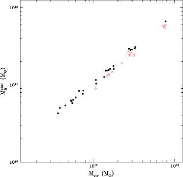
Figure 1: Masses at the halo scale of stars versus their corresponding virial masses. filled black symbols: SF-A sample ELOs; open red symbols: SF-B sample ELOs

An important point is the amount of gas infall relative to the halo mass scale. As illustrated in Figure 2 for $M_{\rm h}^{\rm cb}/M_{\rm vir}$, any of the ratios $M_{\rm h}^{\rm ab}/M_{\rm vir}$, $M_{\rm h}^{\rm cb}/M_{\rm vir}$ or $M_{\rm h}^{\rm star}/M_{\rm vir}$ decreases as $M_{\rm vir}$ increases, as observationally found at smaller scales (see $\S$1). Note that we have in any case $M_{\rm h}^{\rm ab}/M_{\rm vir}<\Omega_{b}/\Omega_{m}=0.171$, the average cosmic fraction, so that there is a lack of baryons within $r_{\rm vir}$ relative to the dark mass content that becomes more important as $M_{\rm vir}$ increases. Otherwise, heating processes along ELO assembly give rise to a hot gas halo around the objects, partially beyond the virial radii. The amount of hot gas mass outside the virial radii, normalised to the ELO stellar mass $M_{\rm bo}^{\rm star}$ (see $\S$3.2), increases with the mass scale. It also increases relative to the cold gas content at the halo scale. To illustrate this point, in Figure 3 we plot the integrated hot gas density profile normalised to the mass of cold baryons inside the virial radii, $M_{\rm h}^{\rm cb}$. The mass effect can be clearly appreciated in this Figure, where we see the following:

(i) The mass of hot gas increases monotonically up to $r\simeq 4r_{\rm vir}$, and maybe also beyond this value, but it is difficult at these large radii to properly dilucidate whether or not a given hot gas mass element belongs to a given ELO or to another close one (to alleviate this difficulty, only those ELOs not having massive neighbours within radii of 6$\times r_{\rm vir}$ have been considered to draw this Figure).

(ii) The hot gas mass fraction increases with $M_{\rm vir}$ at given $r/r_{\rm vir}$. This suggests that the cold baryons that massive ELOs miss inside $r_{\rm vir}$ relative to less massive ones appear as a diffuse warm component at the outskirts of their configurations.

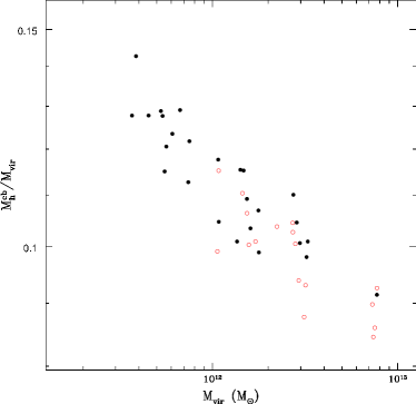
Figure 2: Masses of cold baryons inside the virial radii in units of the corresponding virial mass for the ELO sample. filled black symbols: SF-A sample ELOs; open red symbols: SF-B sample ELOs.

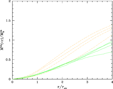
Figure 3: The hot gas density profile normalised to the mass of cold baryons inside the virial radii for isolated ELOs. Orange point-dashed lines: ELOs in the mass interval $1.5\times 10^{12}$ M${}_{\odot}\leq M_{\rm vir}<5\times 10^{12}$ M_⊙; continuous green lines: ELOs in the mass interval $M_{\rm vir}<1.5\times 10^{12}$ M_⊙.

We now comment on length scales. The overall half-mass radii $r_{\rm e,h}^{\rm tot}$ are closely correlated to $M_{\rm vir}$. Concerning baryon mass distributions, dissipation in shocks and gas cooling play now important roles to determine these mass distributions. And so, the $r_{\rm e,h}^{\rm star}$ radii depend on how much energy was radiated before gaseous particles became dense enough to be turned into stars. This, in turn, depends on the mass scale, on the one hand, and, in a given mass range, on the values of SF parameters, on the other hand. And so, more massive ELOs tend to have larger $r_{\rm e,h}^{\rm star}$ radii and, in a given mass range, SF-A sample ELOs tend to have larger $r_{\rm e,h}^{\rm star}$ radii than their SF-B sample counterparts, because the SF implementation in the code demands denser gas to form stars in the later than in the former. This effect is more remarkable for sizes at the scale of the baryonic object, as we shall see in the next subsection.

3.2 Masses and Sizes at the Scale of the Baryonic Object

Let us now turn to the study of ELOs at the scale of the baryonic objects themselves, that is, at scales of some tens of kpcs. Physically, the mass parameter at the ELO scale is $M_{\rm bo}^{\rm cb}$, the total amount of cold baryons that have reached the central volume of the haloes, forming an ELO. Most of these cold baryons have turned into stars, depending on the strength of the dynamical activity in the volume surrounding the proto-ELO at high $z$, and, also, on the values of the SF parameters. $M_{\rm bo}^{\rm star}$ is the stellar mass. It can be estimated from luminosity data through modelling (see Kauffmann et al. 2003a, for example). Effective or half-mass radii at the baryonic object scale, $r_{\rm e,bo}^{\rm cb}$ and $r_{\rm e,bo}^{\rm star}$, can be defined as those radii enclosing half the $M_{\rm bo}^{\rm cb}$ or $M_{\rm bo}^{\rm star}$ masses, respectively. These are the relevant size scales for the intrinsic ELOs, but the observationally relevant size scales are the projected half-mass radii. They are determined from $M_{\rm cyl}(R)$, the integrated projected mass density in concentric cylinders of radius $R$ for the different constituents. For example, $R_{\rm e,bo}^{\rm cb}$ and $R_{\rm e,bo}^{\rm star}$ are the projected radii where $M^{\rm cb}_{\rm cyl}(R)$ and $M^{\rm star}_{\rm cyl}(R)$ are equal to $M_{\rm bo}^{\rm cb}/2$ and to $M_{\rm bo}^{\rm star}/2$, respectively. Significant parameters at the baryonic object scale are listed in Table 4. Note that ELOs have a lower limit in their stellar mass content of 3.8 $\times$ 10¹⁰ M_⊙ (see Kauffmann et al. 2003b for a similar result in SDSS early-type galaxies).

Table 4: Masses, sizes and mean square velocities at the baryonic object scale, as well as projected radii and central stellar l.o.s. velocity dispersions ($z=0$)

Run	ELO	$M_{\rm bo}^{\rm cb}$	$M_{\rm bo}^{\rm star}$	$r_{\rm e,bo}^{\rm star}$	$R_{\rm e,bo}^{\rm star}$	$\sigma_{\rm 3,bo}^{\rm star}$	$\sigma_{\rm los,0}^{\rm star}$
8714	#173	43.12	42.59	13.01	12.72	351.93	226.67
	#353	25.62	25.17	8.25	7.95	297.11	192.47
	#581	13.72	13.45	6.75	6.66	222.42	136.18
	#296	12.21	11.95	4.76	4.69	225.95	138.39
	#373	7.38	7.23	3.85	3.83	186.95	116.88
	#772	5.62	5.51	2.33	2.30	181.59	107.28
	#284	5.70	5.48	2.81	2.74	169.09	103.74
8747	#288	20.11	20.05	7.84	7.81	269.58	171.50
	#115	12.21	12.17	2.94	2.96	259.05	161.63
	#189	4.74	4.68	2.57	2.61	169.93	104.81
	#915	4.52	4.32	2.23	2.19	164.69	99.61
8741	#011	19.10	19.10	5.36	5.35	279.61	174.62
	#017	10.34	10.15	4.15	4.09	224.37	139.54
	#930	8.95	8.85	4.68	4.70	214.97	138.64
	#945	10.00	9.89	4.58	4.62	209.68	128.84
	#097	9.46	9.34	5.00	5.05	206.21	132.19
	#907	5.63	5.55	2.57	2.60	187.67	119.71
8742	#234	27.42	27.13	9.33	9.23	287.18	190.47
	#283	13.51	13.44	4.28	4.30	246.54	151.56
	#254	10.91	10.81	4.50	4.50	221.72	134.23
	#092	6.55	6.38	3.14	3.17	177.69	108.46
8743	#238	20.97	20.88	6.76	6.79	289.43	181.53
	#328	7.76	7.60	3.40	3.36	187.15	116.49
	#515	5.74	5.63	2.60	2.62	185.04	114.13
	#437	4.79	4.70	2.36	2.40	172.71	105.13
	#421	3.91	3.81	2.11	2.14	161.41	102.09
8716	#173	39.13	38.07	7.07	6.75	355.08	237.07
	#253	22.98	22.54	4.40	4.28	305.37	199.34
	#581	13.03	12.46	3.35	3.18	243.71	152.89
	#296	10.87	10.43	2.52	2.50	241.58	140.14
8717	#317	42.28	41.55	8.12	7.77	387.30	223.73
	#288	18.63	18.25	3.48	3.45	286.59	169.81
	#348	15.36	14.84	3.73	3.57	261.06	158.31
8721	#011	21.73	21.37	3.34	3.31	287.47	177.04
	#945	9.99	9.30	2.55	2.44	226.33	128.90
	#097	8.62	8.34	2.34	2.36	213.00	133.46
8722	#293	43.56	42.75	9.40	9.09	365.95	215.68
	#234	22.40	22.28	3.53	3.57	313.03	196.62
	#283	12.67	12.51	2.10	2.13	262.81	163.89
	#254	11.97	11.52	2.64	2.62	237.10	137.68
8723	#647	34.01	33.43	5.86	5.76	336.69	210.25
	#238	20.09	19.91	3.78	3.74	297.51	191.05
	#563	13.67	13.44	2.41	2.45	274.84	164.01

Masses are given in 10¹⁰ M_⊙, distances in kpc, velocity dispersions in km s^-1.

To illustrate how the halo total mass, $M_{\rm vir}$, determines the ELO structure at kpc scales, in Figures 4 and 5 we draw $M_{\rm bo}^{\rm star}$ and $r_{\rm e,bo}^{\rm star}$ versus $M_{\rm vir}$, respectively, for the ELO sample. A good correlation is apparent in Figure 4, where it is shown that ELO stellar masses are mainly determined by the halo mass scale, $M_{\rm vir}$, with only a very slight dependence on the SF parametrisation (SF-A type ELOs have a slightly higher stellar content than their SF-B counterparts, as expected). Figure 5 shows also a good correlation between the length scales for the stellar masses and $M_{\rm vir}$, but now the sizes depend also on the SF parameters. The physical foundations of this behaviour are the same as discussed in $\S$3.1.

The observationally relevant scalelengths are the projected half-mass radii $R_{\rm e,bo}^{\rm star}$. Their correlations with their intrinsic three dimensional counterparts $r_{\rm e,bo}^{\rm star}$ are very good, as illustrated in Figure 6, where the very low dispersion in the plots of the $c_{\rm rp}\equiv r_{\rm e,bo}^{\rm star}/R_{\rm e,bo}^{\rm star}$ ratios versus the stellar mass $M_{\rm bo}^{\rm star}$ can be appreciated. The results of a fit to a power law of the form $c_{\rm rp}=A_{\rm rp}(M_{\rm bo}^{\rm star})^{\beta_{\rm rp}}$ are given in Table 5 , where we see that the $c_{\rm rp}$ ratios show a very mild mass dependence in the SF-A sample and none in the SF-B sample. This result is important because it indicates that the observationally available projected radii $R_{\rm e,bo}^{\rm star}$ are robust estimators of the physically meaningful size scales $r_{\rm e,bo}^{\rm star}$.

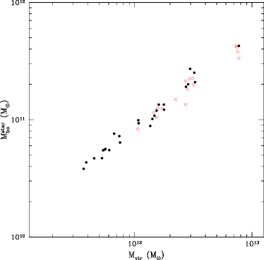
Figure 4: Stellar masses at the baryonic object scale scale versus halo mass for the ELO sample. Symbols are as in previous Figures

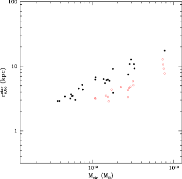
Figure 5: The 3D half-mass radii for stellar masses at the baryonic object scale versus halo mass for the ELO sample. Symbols are as in previous Figures

Figure 6: The $c_{\rm rp}\equiv r_{\rm e,bo}^{\rm star}/R_{\rm e,bo}^{\rm star}$ ratios versus the stellar masses at the baryonic object scale. Symbols are as in previous Figures.

We now address the correlations of normalised mass and size scales. The increasing behaviour of the $M_{\rm vir}/M_{\rm bo}^{\rm cb}$ and $M_{\rm vir}/M_{\rm bo}^{\rm star}$ ratios with increasing mass scale are very interesting. In particular, the last ratio (Figure 7) follows the same trends as the empirical $M_{\rm e}/L$ versus $L$ relation, see Bernardi et al. 2003b. The results of a fit to a power law of the form $M_{\rm vir}/M_{\rm bo}^{\rm star}=A_{\rm vir}(M_{\rm bo}^{\rm star})^{\beta_{\rm vir}}$ are given in Table 5, where we see that they do not depend on the SF parameterisation.

Table 5: Slopes for Linear Fits

	SF-A		SF-B
$M_{1}$	0.256	$\pm$ 0.035	0.281	$\pm$ 0.048
$\beta_{\rm vir}$	0.221	$\pm$ 0.083	0.237	$\pm$ 0.158
$\beta_{\rm M}$	-0.204	$\pm$ 0.116	-0.247	$\pm$ 0.189
$\beta_{\rm F}$	0.025	$\pm$ 0.048	0.022	$\pm$ 0.081
$\beta_{\rm vd}$	0.021	$\pm$ 0.041	0.076	$\pm$ 0.075
$\beta_{\rm vpc}$	-0.044	$\pm$ 0.029	-0.044	$\pm$ 0.093
$\beta_{\rm rd}$	-0.225	$\pm$ 0.127	-0.316	$\pm$ 0.199
$\beta_{\rm rp}$	0.019	$\pm$ 0.009	0.016	$\pm$ 0.017

Column 2: the slopes of the $\kappa_{3}^{\rm D}=M_{1}\kappa_{1}^{\rm D}+M_{0}$ relation (direct fits); the slopes of the $M_{\rm vir}/M_{\rm bo}^{\rm star}$ and $c_{\rm i}\propto(M_{\rm bo}^{\rm star})^{\beta_{\rm i}}$ scaling relations for the the SF-A sample, calculated in $\log-\log$ plots through direct fits. Column 3: their respective 95% confidence intervals. Columns 4 and 5: same as columns 2 and 3 for the SF-B sample.

To have an idea on how important cold baryon infall has been at the baryonic object scale relative to that at the halo scale, in Figure 8 the $M_{\rm h}^{\rm cb}/M_{\rm bo}^{\rm cb}$ ratios are drawn as a function of the ELO mass scale. We see that in any case more than half the mass of cold baryons inside the virial radii are concentrated in the central baryonic object, and that there is a mass effect in the sense that this fraction grows with decreasing ELO mass scale, and no appreciable SF effect.

Concerning sizes, in Figure  9 we plot the $c_{\rm rd}\equiv r_{\rm e,h}^{\rm tot}/r_{\rm e,bo}^{\rm star}$ ratios versus the $M_{\rm bo}^{\rm star}$ mass scale for ELOs in both the SF-A and the SF-B samples. In this Figure the effects of SF parameterisation are clear: SF-A type ELOs have larger sizes relative to the halo size than SF-B type ELOs. There is also a clear mass effect, with more massive ELOs less concentrated relative to the total mass distribution than less massive ones (i.e., spatial homology breaking; note, however that the scatter is important). Moreover, Figure  9 suggests that this trend does not significantly depend on the SF parametrisation. These indications are quantitatively confirmed through a fit to a power law $c_{\rm rd}=A_{\rm rd}(M_{\rm bo}^{\rm star})^{\beta_{\rm rd}}$ (see Table 5) and have interesting implications to explain the tilt of the observed FP.

Figure 7: The $M_{\rm vir}/M_{\rm bo}^{\rm star}$ ratios as a function of the ELO mass scale. Symbols are as in previous Figures

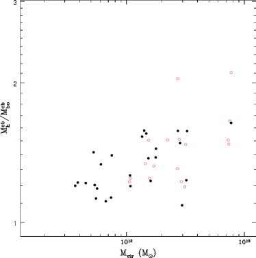
Figure 8: The $M_{\rm h}^{\rm cb}/M_{\rm bo}^{\rm cb}$ ratios as a function of the ELO mass scale. Symbols are as in previous Figures

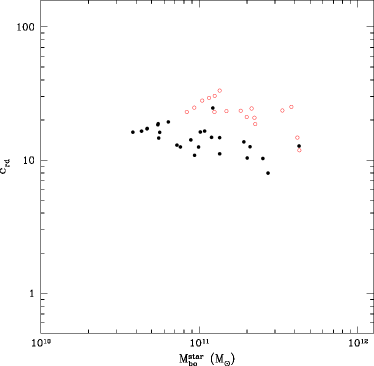
Figure 9: The $c_{\rm rd}\equiv r_{\rm e,h}^{\rm tot}/r_{\rm e,bo}^{\rm star}$ ratios as a function of the ELO mass scale. Symbols are as in previous Figures. Spatial homology breaking is clear in this Figure

4 Kinematics

4.1 Three-dimensional velocity distributions

Shapes and mass density profiles (i.e., positions) are related to the 3D velocity distributions of relaxed E galaxies through the Jeans equation (see Binney & Tremaine 1987). Observationally, the informations on such 3D distributions is not available for external galaxies, only the line-of-sight velocity distributions (LOSVD) can be inferred from their spectra. They have been found to be close to gaussian (Binney & Tremaine 1987; van der Marel & Franx 1993), so that simple equilibrium models can be expected to adequately describe their dynamical state (de Zeeuw & Franx 1991). The complete six dimensional phase space informations for each of the particles sampling the ELOs provided by numerical simulations, allow us to calculate the velocity profiles, $V_{\rm cir}(r)$, the 3D profiles for the velocity dispersion, $\sigma_{\rm 3D}(r)$, and their corresponding anisotropy profiles. The anisotropy is defined as:

$$\beta_{\rm ani}=1-\frac{\sigma^{2}_{\rm t}}{2\,\sigma^{2}_{\rm r}},$$ (4)

where $\sigma_{\rm r}$ and $\sigma_{\rm t}$ are the radial and tangential velocity dispersions ($\sigma_{\rm t}^{2}=\sigma_{\theta}^{2}+\sigma_{\phi}^{2}$), relative to the centre of the object. These profiles, as well as the LOS velocity $V_{\rm los}(R)$ and LOS velocity dispersion $\sigma_{\rm los}(R)$ profiles, are analysed in detail in Oñorbe et al., in preparation. Figure 10 illustrates the more outstanding results we have obtained: ELO velocity dispersion profiles in three dimensions are slightly decreasing for increasing $r$, both for dark matter and stellar particles, $\sigma^{\rm dark}_{3D}(r)$ and $\sigma^{\rm star}_{3D}(r)$. It has been found that $(\sigma^{\rm dark}_{3D}(r))^{2}\sim$ (1.4 – 2) $(\sigma^{\rm star}_{3D}(r))^{2}$, as Loewenstein 2000 had found on theoretical grounds. This is so because stars are formed from gas that had lost energy by cooling. This result on kinematical segregation is very interesting because it has the implication that the use of stellar kinematics to measure the total mass of ellipticals could result into inaccurate values. The study of anisotropy has shown that it is always positive and almost non-varying with $r$ (recall, however, that ELOs are non-rotating and that they have been identified as dynamically relaxed objects, so that there are not recent mergers in our samples). The stellar component generally shows more anisotropy than the dark component, maybe coming from the radial motion of the gas particles that gave rise to the stars.

Figure 10: The $\sigma_{\rm 3D}(r)$ profiles of a typical ELO in the SF-A sample. Also shown are their anisotropy profiles $\beta_{\rm ani}(r)$. Long-dashed lines: dark matter; short-dashed lines: stars

4.2 Global parameters for the velocity distribution

Only for a limited number of ellipticals are the $V_{\rm los}(R)$ or $\sigma_{\rm los}(R)$ profiles available. Observationally, a useful characterisation of the velocity dispersion of an E galaxy is provided by its central stellar line-of-sight velocity dispersion, $\sigma_{\rm los,0}$. It corresponds to the velocity dispersion of the stellar (as opposed to dark matter or other) component. Due to its interest, $\sigma_{\rm los,0}$ has deserved an important attention in literature and it had been measured for several E galaxy samples before the SDSS results (Faber et al. 1987; Djorgovski & Davis 1987; Dressler et al. 1987; Lucey, Bower & Ellis 1991; Jørgensen, Franx & Kjoergaard 1993; Jørgensen et al. 1996; Kelson et al. 1997; Kelson et al. 2000, Bernardi et al. 2002). In Table 4 the values of $\sigma_{\rm los,0}^{\rm star}$ for the ELO sample are listed. In Figure 11 we show the good correlation between $\sigma_{los,0}^{star}$ and the virial mass, $M_{vir}$.

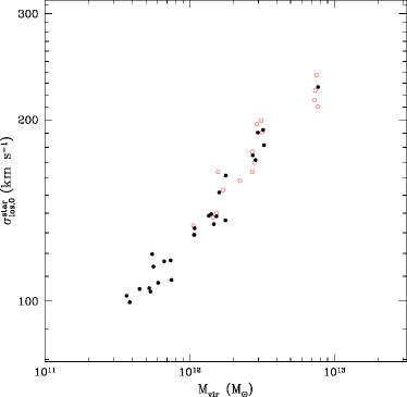
Figure 11: The correlation between the central l.o.s.  velocity dispersion and the virial mass for the ELO samples. Symbols are as in previous Figures.

Physically, a measure of the average dynamical state of stars in the ELO itself is provided by their mean square velocity relative to the ELO center of mass, or average three-dimensional velocity dispersion $\sigma_{\rm 3,bo}^{\rm star}$, of which the observationally available $\sigma_{\rm los,0}^{\rm star}$ parameter is assumed to be a fair estimator. To test this point, in Figure 12 we plot the $c_{\rm vpc}\equiv(\sigma_{\rm 3,bo}^{\rm star})^{2}/3(\sigma_{\rm los,0}^{\rm star})^{2}$ ratios versus the ELO mass scale. We see that no mass effect is apparent, and this is quantitatively confirmed in Table 5, where the results of a fit of the form $c_{\rm vpc}=A_{\rm vpc}(M_{\rm bo}^{\rm star})^{\beta_{\rm vpc}}$ are given. We also see that due to radial anisotropy, $c_{\rm vpc}<1$, with no SF parametrisation effect. So, there is not mass bias when using $\sigma_{\rm los,0}^{\rm star}$ as an estimator for $\sigma_{\rm 3,bo}^{\rm star}$, but some warnings are in order concerning anisotropy effects.

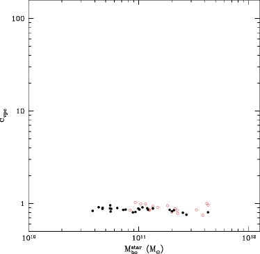
Figure 12: $c_{\rm vpc}\equiv(\sigma_{\rm 3,bo}^{\rm star})^{2}/3(\sigma_{\rm los,0}^{\rm star})^{2}$ ratios versus the ELO mass scale. Symbols are as in previous Figures

A significant velocity dispersion parameter for ELOs at the halo scale is $\sigma_{\rm 3,h}^{\rm tot}$, the average 3-dimensional velocity dispersion of the whole elliptical, including both dark and baryonic matter. According with Eq. 2, this is the velocity dispersion entering in the virial theorem for the whole ELO configuration. To test that this is in fact the case, in Figure 13 we plot the $c_{\rm F}\equiv GM_{\rm vir}/(\sigma_{\rm 3,h}^{\rm tot})^{2}r_{\rm e,h}^{\rm tot}$ form factors (see Eq. 2) as a function of $M_{\rm bo}^{\rm star}$. The lack of any significant mass or SF parametrisation effects in this Figure are quantitatively confirmed through a fit to power laws of the form $c_{\rm F}=A_{\rm F}(M_{\rm bo}^{\rm star})^{\beta_{\rm F}}$, whose results in Table 5 are consistent with $c_{\rm F}$ being independent of the ELO mass scale or SF parameter values. Note also that the $c_{\rm F}$ values are as expected (Binney & Tremaine 1987).

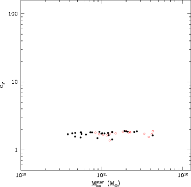
Figure 13: The $c_{\rm F}\equiv GM_{\rm vir}/(\sigma_{\rm 3,h}^{\rm tot})^{2}r_{\rm e,h}^{\rm tot}$ form factors (see Eq. 2) versus the ELO mass scale. Symbols are as in previous Figures. This Figure confirms that $r_{\rm e,h}^{\rm tot}$ and $\sigma_{\rm 3,h}^{\rm tot}$ are the size and velocity dispersion ELO parameters that must be used in the virial theorem

Once we have confirmed that when writting the virial theorem for an ELO configuration, $\sigma_{\rm 3,h}^{\rm tot}$ is the velocity dispersion one has to use, let us remind that one has to be careful when using $\sigma_{\rm los,0}^{\rm star}$ or $\sigma_{\rm 3,bo}^{\rm star}$ as estimators for this physically meaningful quantity. In Figure 14 we plot the $c_{\rm vd}\equiv(\sigma_{\rm 3,h}^{\rm tot}/\sigma_{\rm 3,bo}^{\rm star})^{2}$ ratios, that measure how dissipation and concentration affect, on average, to the relative values of the dispersion at the halo scale (involving also dark matter) and at the baryonic object scale. No mass effects are apparent in this Figure, but an average kinematical segregation is clear, (see Table 5 for the results of a fit to the expression $c_{\rm vd}=A_{\rm vd}(M_{\rm bo}^{\rm star})^{\beta_{\rm vd}}$). These are important results, which could have interesting observational implications.

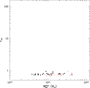
Figure 14: The $c_{\rm vd}\equiv(\sigma_{\rm 3,h}^{\rm tot}/\sigma_{\rm 3,bo}^{\rm star})^{2}$ ratios (average kinematical segregation) as a function of the ELO mass scale. Symbols are as in previous Figures. No dynamically broken homology can be seen in this Figure, but the kinematical segregation between dark matter and stars is clear.

5 The Intrinsic Dynamical Planes and the Dynamical Fundamental Planes

5.1 The dynamical plane relations of ELO samples

In the last section it has been shown that the mass, size and velocity dispersion parameters at the halo scale satisfy virial relations. This result is, however, at odds with the tilt of the observed FP of ellipticals discussed in $\S$1, that involves the $L$, $R_{\rm e}^{\rm light}$ and $\sigma_{\rm los,0}$ observed variables, whose virtual counterparts describe the ELO at the scale of the baryonic object. So, we have first to analyse whether or not the mass, size and velocity dispersion of ELOs at this scale define planes tilted relative to the virial one.

To this end, we have carried out a principal component analysis (PCA) of the SF-A and SF-B samples in the three dimensional variables $E\equiv\log_{10}M_{\rm bo}^{\rm star}$, $r\equiv\log_{10}r_{\rm e,bo}^{\rm star}$ and $v\equiv\log_{10}\sigma_{\rm 3,bo}^{\rm star}$ through their $3\times 3$ correlation matrix C. We have used three dimensional variables rather than projected ones to circumvent projection effects, that add noise to the correlations (see, for example, Figure 12). We have found that, irrespective of the SF parametrisation, one of the eigenvalues of C is considerably smaller than the others (see Table 6), so that ELOs populate in any case a flattened ellipsoid close to a two-dimensional plane in the $(E,r,v)$ space that we call the intrinsic dynamical plane (IDP); the FP is the observed manifestation of this IDP. The eigenvectors of C indicate that the projection

$$E-\textit{\~{E}}=\alpha^{\rm 3D}(r-\textit{\~{r}})+\gamma^{\rm 3D}(v-\textit{\~{v}}),$$ (5)

where $\textit{\~{E}},\textit{\~{r}}$ and ṽ are the mean values of the $E,r$ and $v$ variables, shows the IDP viewed edge-on. Table 6 gives the eigenvalues of the correlation matrix C ($\lambda_{1}$, $\lambda_{2}$, $\lambda_{3}$), the planes eq. (5), as well as their corresponding thicknesses $\sigma_{\it Erv}$, both for the SF-A and SF-B samples. The IDPs are in fact tilted relative to the virial plane (characterized by $\alpha=1,\gamma=2$), and their scatter is very low as measured by their thicknesses $\sigma_{\it Erv}$. Note that the eigenvalues of the PCA analysis are not dependend on the SF parametrisation.

Table 6: Results of PCA at z=0

Sample	No.	Ẽ	r̃	ṽ	$\lambda_{1}$	$\lambda_{2}$	$\lambda_{3}$	$\alpha^{\rm 3D}$	$\gamma^{\rm 3D}$	$\sigma_{\rm Erv}$
SF-A	26	10.993	0.746	2.335	0.12893	0.00355	0.00013	0.427	2.066	0.011
SF-B	17	11.259	0.695	2.453	0.09342	0.00292	0.00014	0.249	2.449	0.012

Column 2: ELO number in the sample.
Columns 3, 4 and 5: sample mean values of the $E,r$ and $v$ variables.
Columns 6, 7 and 8: eigenvalues of the correlation matrix.
Columns 9 and 10: coefficients of the plane (Eq. (5)).
Column 11: IDP scatter in the $E,r$ and $v$ variables.

In Figure 15 we plot the $(E,v),(E,r)$ and $(r,v)$ projections of the IDPs corresponding both to the SF-A sample and the SF-B sample. We see that the three projections show correlations and that these are very tight for the first of them.

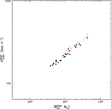
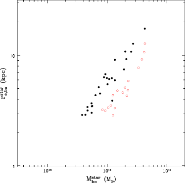
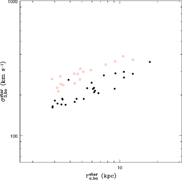
Figure 15: The IDPs for the SF-A and SF-B samples. Projections on the $(E,v)$, $(E,r)$ and $(r,v)$ coordinate planes are shown.

5.2 Comparing the IDP to the observed FP of elliptical galaxies

The next step is to compare the results on the IDPs we have found with the tilt and the scatter of the observed FP. We note that the $r$ and $v$ variables are not observationally available, so that we have to use their projected counterparts. Assuming that the projected stellar mass density profile, $\Sigma^{\rm star}(R)$, can be taken as a measure of the surface brightness profile, then $<\Sigma^{\rm star}>_{\rm e}=c<I^{\rm light}>_{\rm e}$, with $c$ a constant, and $R_{\rm e,bo}^{\rm star}\simeq R_{\rm e}^{\rm light}$ and we can look for a fundamental plane (hereafter, the dynamical FP) in the 3-space of the structural and dynamical parameters $R_{\rm e,bo}^{\rm star}$, $<\Sigma^{\rm star}>_{\rm e}$ and $\sigma^{\rm star}_{\rm los,0}$, directly provided by the hydrodynamical simulations. To make this analysis as clear as possible, we transform to a $\kappa$-like orthogonal coordinate system, the dynamical $\kappa_{i}^{\rm D}$ system, $i$=1,2,3, similar to that introduced by Bender, Burstein & Faber (1992), but using $R_{\rm e,bo}^{\rm star}$ instead of $R_{\rm e}^{\rm light}$ and $<\Sigma^{\rm star}>_{\rm e}$ instead of $<I^{\rm light}>_{\rm e}$, and, consequently, free of age, metallicity or IMF effects. The dynamical $\kappa_{i}^{\rm D}$ variables can be written as:

$$\kappa_{1}^{D}\equiv[\log\left(\sigma^{\rm star}_{\rm los,0}\right)^{2}+\log R_{\rm e,bo}^{\rm star}]/\sqrt{2}$$ (6)

$$\kappa_{2}^{D}\equiv[\log\left(\sigma^{\rm star}_{\rm los,0}\right)^{2}+2\log\langle\Sigma^{\rm star}\rangle_{\rm e}-\log R_{\rm e,bo}^{\rm star}]/\sqrt{6}$$ (7)

$$\kappa_{3}^{D}\equiv[\log\left(\sigma^{\rm star}_{\rm los,0}\right)^{2}-\log\langle\Sigma^{\rm star}\rangle_{e}-\log R_{\rm e,bo}^{\rm star}]/\sqrt{3}$$ (8)

and they are related to the $\kappa$ coordinates through the expressions: $\kappa_{1}\simeq\kappa^{\rm D}_{1}$, $\kappa_{2}\simeq\kappa^{\rm D}_{2}-\sqrt{6}/3\log(M_{\rm bo}^{\rm star}/L)$ and $\kappa_{3}\simeq\kappa^{\rm D}_{3}+\sqrt{3}/3\log(M_{\rm bo}^{\rm star}/L)$. We discuss the tilt and the scatter of the dynamical FP separately. We first address the tilt issue. We use at this stage for the $R_{\rm e,bo}^{\rm star}$ and $\sigma^{\rm star}_{\rm los,0}$ variables the averages over three orthogonal l.o.s. projections, to minimize the scatter in the plots caused by projection effects.

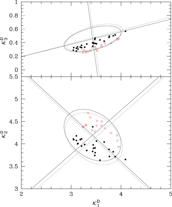
Figure 16: Dynamical Fundamental Plane in $\kappa^{D}$ system. Edge-on projection (top panel) and nearly face-on projection (bottom panel) of the dynamical FP of ELOs in the $\kappa^{D}$ variables (black filled symbols: SF-A sample; red open symbols: SF-B sample). We also draw the respective concentration ellipses (with their major and minor axes) for the SDSS early-type galaxy sample from Bernardi et al. (2003b) in the z band (solid line) and the r band (dashed line). See text for more details.

Figure 16 plots the $\kappa_{3}^{\rm D}$ versus $\kappa_{1}^{\rm D}$ (top) and $\kappa_{2}^{\rm D}$ versus $\kappa_{1}^{\rm D}$ (bottom) diagrams for ELOs in both the SF-A and SF-B samples. We also drew the 2$\sigma$ concentration ellipses in the respective variables, as well as its major and minor axes, for the SDSS early-type galaxy sample in the SDSS $z$ band (solid lines) and in the $r$ band (point lines) as analysed by Bernardi et al. 2003b, 2003c. The most outstanding feature of this Figure (upper panel) is the good scaling behaviour of $\kappa_{3}^{\rm D}$ versus $\kappa_{1}^{\rm D}$, with a very low scatter (see the slopes $M_{1}$ in Table 5; note that the slopes for the SF-A and SF-B samples are consistent within their errors, while the zero-points depend on the SF parameterisation through the ELO sizes). Another interesting feature of Figure 16 is that it shows that most of the values of the $\kappa_{i}^{\rm D}$ coefficients are within the 2$\sigma$ concentration ellipses in both plots for ELOs formed in SF-A type simulations, with a slightly worse agreement for ELOs in the SF-B sample. This means that ELOs have counterparts in the real world (Sáiz et al. 2004). It is worth mentioning that these results are stable against slight changes in the values of the $\Omega_{\Lambda}$, $\Omega_{\rm baryon}$ or $h$ parameters; for example, we have tested that using their preferred WMAP values (Spergel et al. 2003) shows results negligibly different to those plotted in Figure 16. Finally, we note that either the dynamical or the observed FPs are not homogeneously populated: both SDSS ellipticals and ELOs occupy only a region within these planes (see Figure 16 lower panel, see also Guzmán et al. 1993; Márquez et al. 2000). This means that, from the point of view of their structure and dynamics, ELOs are a two-parameter family where the two parameters are not fully independent. Moreover, concerning ELOs, the occupied region changes when the SF parameters change. The reason of this change is that the ELO sizes decrease as SF becomes more difficult, because the amount of dissipation experienced by the stellar component along ELO assembly increases.

We now turn to consider the scatter of the dynamical FP for the ELO samples and compare it with the scatter of the FP for the SDSS elliptical sample, calculated as the square root of the smallest eigenvalue of the 3$\times$3 covariance matrix in the $E$ (or $\log L$), $V\equiv\log\sigma_{\rm los,0}^{\rm star}$ and $R\equiv\log R_{\rm e,bo}^{\rm star}$ variables (Saglia et al. 2001). As Figure 16 suggests, when projection effects are circumvented by taking averages over different directions, the resulting three dimensional orthogonal scatter for ELOs is smaller than for SDSS ellipticals ($\sigma_{\it EVR}=0.0164$ and $\sigma_{\it EVR}=0.0167$ for the SF-A and SF-B samples, respectively, to be compared with $\sigma_{\it LVR}=0.0489$ for the SDSS in the $\log L,V\equiv\log\sigma_{\rm los,0}$ and $R\equiv\log R_{\rm e}^{\rm light}$ variables). To estimate the contribution of projection effects to the observed scatter, we have calculated the orthogonal scatter for ELOs when no averages over projection directions for the $R_{\rm e,bo}^{\rm star}$ and $\sigma_{\rm los,0}^{\rm star}$ variables are made. The scatter ($\sigma_{\it EVR}=0.0238$ and $\sigma_{\it EVR}=0.0214$ for the SF-A and SF-B samples) increases, but it is still lower than observed. This indicates that a contribution from stellar population effects is needed to explain the scatter of the observed FP, as suggested by different authors (see, for example, Pahre et al. 1998; Trujillo et al. 2004).

5.3 Clues on the physical origin of the IDP tilt

We now address the issue of the physical origin of the tilt of ELO IDPs relative to the virial relation. As discussed in $\S$1, a non-zero tilt can be caused by a mass dependence of the mass-to-light ratio $M_{\rm vir}/L$, of the mass structure coefficients $c_{\rm M}^{\rm vir}\equiv{GM_{\rm vir}\over 3\sigma_{\rm los,0}^{2}R_{\rm e}^{\rm light}}$, or of both of them. We examine these possibilities in turn.

i) We first note that the mass-to-light ratio can be written as:

$$M_{\rm vir}/L=A_{\rm vir}(M_{\rm bo}^{\rm star})^{\beta_{\rm vir}}\times\gamma^{\rm star},$$ (9)

where $\gamma^{\rm star}\equiv M_{\rm bo}^{\rm star}/L$ is the stellar mass-to-light ratio, that, as already explained, can be considered to be independent of the E galaxy luminosity or ELO mass scale. Figure 7 and the values of the $\beta_{\rm vir}$ slopes given in Table 5, indicate that the dark to bright mass content of ELOs increases with their mass, contributing a tilt to their IDPs. Similar results have also been found in pre-prepared simulations of dissipative mergers (Robertson et al. 2006).

ii) Writting the $c_{\rm M}^{\rm vir}$ mass structure coefficients as power laws $c_{\rm M}^{\rm vir}=A_{\rm M}(M_{\rm bo}^{\rm star})^{\beta_{\rm M}}$, ELO homology would imply ${\beta_{\rm M}}=0$. To elucidate whether or not this is the case, the ${\beta_{\rm M}}$ slopes have been measured on the ELO samples through direct fits in log-log scales. The results are given in Table 5, where we see that the homology is in fact broken both for SF-A or SF-B samples. To deepen into the causes of this behaviour, we use Eqs. 2 and 3 to write

$$c_{\rm M}^{\rm vir}=c_{\rm F}c_{\rm rd}c_{\rm rp}c_{\rm vd}c_{\rm vpc},$$ (10)

where the $c_{\rm i}$ coefficients, with i = rd, rp, vd, vpc have been defined in $\S$3.2, and with i = F in $\S$4.2. Taking into account the power-law forms of these coefficients, we have:

$$\beta_{\rm M}=\beta_{\rm F}+\beta_{\rm rd}+\beta_{\rm rp}+\beta_{\rm vd}+\beta_{\rm vpc},$$ (11)

when the $\beta_{\rm i}$ slopes are calculated through direct fits. From Table 5 we see that the main contribution to the homology breaking comes from the $c_{\rm rd}$ coefficients (i.e., spatial homology breaking, see $\S$3.2 and Oñorbe et al. 2005), while, as previously discussed, no dynamical homology breaking (see $\S$4.2) or projection effects are important in our ELO samples.

6 Summary, discussion and conclusions

6.1 Summary

We present an analysis of the sample of ELOs formed in ten different cosmological simulations, run within the same global flat $\Lambda$ cosmological model, roughly consistent with observations. The normalisation parameter has been taken slightly high, $\sigma_{8}=1.18$, as compared with the average fluctuations of 2dFGRS or SDSS galaxies to mimic an active region of the Universe. Newton laws and hydrodynamical equations have been integrated in this context, with a standard cooling algorithm and a star formation parameterization through a Kennicutt-Schmidt-like law, containing our ignorance about its details at sub-kpc scales. No further hypotheses to model the assembly processes have been made. Individual galaxy-like objects naturally appear as an output of the simulations, so that the physical processes underlying mass assembly can be studied. Five out of the ten simulations (the SF-A type simulations) share the SF parameters and differ in the seed used to build up the initial conditions. To test the role of SF parameterisation, the same initial conditions have been run with different SF parameters making SF more difficult, contributing another set of five simulations (the SF-B type simulations). ELOs have been identified in the simulations as those galaxy-like objects at $z=0$ having a prominent, non-rotating dynamically relaxed spheroidal component made out of stars, with no extended discs and very low gas content. These stellar component is embedded in a dark matter halo that contributes an important fraction of the mass at distances from the ELO centre larger than $\sim 10-15$ kpc. No ELOs with stellar masses below 3.8 $\times$ 10¹⁰ M_⊙ or virial masses below 3.7 $\times$ 10¹¹ M_⊙ have been found that met the selection criteria (see Kauffmann et al. 2003b for a similar result in SDSS galaxies and Dekel & Birnboim 2006, and Cattaneo et al. 2006 for a possible physical explanation). ELOs have also an extended halo of hot, diffuse gas. Stellar and dark matter particles constitute a dynamically hot component with an important velocity dispersion, and, except in the very central regions, a positive anisotropy.

The informations about position and velocity distributions of the ELO particles of different kinds (dark matter, stars, cold gas, hot gas) provided by the simulations, allows a detailed study of their intrinsical three dimensional mass and velocity distributions, as well as a measure of the parameters characterising their structure and dynamics. In a forthcoming paper, we report on the three dimensional mass density, circular velocity and velocity dispersion profiles, as well as the projected stellar mass density profiles and the LOS velocity dispersion profiles. In this paper we focus on a parameter analysis to quantify some of the previous results.

Mass, size and velocity dispersion scales for their different components have been measured in the ELO samples, both at the scale of their halo and at the scale of the baryonic object (a few tens of kiloparsecs). At the halo scale, the masses of both cold gas and stars, $M_{\rm h}^{\rm cb}$ and $M_{\rm h}^{\rm star}$, respectively, have been found to be tightly correlated with the halo total mass, $M_{\rm vir}$, with the ratios $M_{\rm h}^{\rm cb}/M_{\rm vir}$ and $M_{\rm h}^{\rm star}/M_{\rm vir}$ decreasing as $M_{\rm vir}$ increases (that is, massive objects miss cold baryons within $r_{\rm vir}$ when compared with less massive ELOs), presumably because gas gets more difficulties to cool and fall as $M_{\rm vir}$ increases. The overall half-mass radii, $r_{\rm e,h}^{\rm tot}$ shows also a very tight correlation with $M_{\rm vir}$. Half-mass radii for the cold baryon or stellar mass distributions have a more complex behaviour, as in these cases gas heating in shocks and energy losses due gas cooling are in competition to determine these distributions.

A very important result we have found when analysing ELOs at the scale of the baryonic object, is that $M_{\rm vir}$ plays an important role to determine the ELO structure also below a few tens of kiloparsecs scales. In fact, both the masses of cold baryons $M_{\rm bo}^{\rm cb}$ (i.e., those baryons that have reached the central regions of the configuration), and of stars $M_{\rm bo}^{\rm star}$, show a good correlation with $M_{\rm vir}$, and, moreover, the $M_{\rm bo}^{\rm cb}/M_{\rm vir}$ and $M_{\rm bo}^{\rm star}/M_{\rm vir}$ ratios (i.e., the relative content of cold baryons or stars versus total mass) decrease as $M_{\rm vir}$ increases. This is the same qualitative behaviour shown by these ratios observationally in the SDSS data, and, also, by ELOs at the halo scale. The dependence of $M_{\rm bo}^{\rm cb}$ or $M_{\rm bo}^{\rm star}$ on the SF parametrisation is only very slight, with SF-A type ELOs having slightly more stars than their SF-B type counterparts. The half-mass radii for cold baryon and stellar masses, $r_{\rm e,bo}^{\rm cb}$ and $r_{\rm e,bo}^{\rm star}$, show also a good correlation with $M_{\rm vir}$, but now the values of the SF parameters also play a role, because their change implies a change in the time interval during which gas cooling is turned on, and this changes the ELO stellar mass distribution, i.e., its lenghthscale, so that ELO compactness increases from SF-A to SF-B type simulations. Another important result is that, regardless of the SF parametrizations used in this work, the relative distributions of the stellar and dark mass components in ELOs show a systematic trend measured through the $c_{\rm rd}\equiv r_{\rm e,h}^{\rm tot}/r_{\rm e,bo}^{\rm star}$ ratios, with stars relatively more concentrated as $M_{\rm vir}$ decreases (i.e., a quantification of the spatial homology breaking). Note that to compare with observational data, the relevant parameters are the projected half-mass radii, $R_{\rm e,bo}^{\rm star}$. We have checked that they show an excellent correlation with the corresponding three dimensional half-mass radii, with the $c_{\rm rp}\equiv r_{\rm e,bo}^{\rm star}/R_{\rm e,bo}^{\rm star}$ ratios showing no significant dependence on the ELO mass scale.

Concerning kinematics, a useful characterisation of the ELO velocity dispersion is the central stellar line-of-sight velocity dispersion, $\sigma_{\rm los,0}^{\rm star}$, whose observational counterpart can be measured from elliptical spectra. A very important result is the very tight correlation we have found between $M_{\rm vir}$ and $\sigma_{\rm los,0}^{\rm star}$, confirming that the observationally measurable $\sigma_{\rm los,0}$ is a fair virial mass estimator. In addition, $\sigma_{\rm los,0}^{\rm star}$ is closely related to the mean square velocity of both, the whole elliptical at the halo scale (including the dark matter), $\sigma_{\rm 3,h}^{\rm tot}$, and the stellar component of the central object, $\sigma_{\rm 3,bo}^{\rm star}$. We have also found that the $c_{\rm vd}\equiv(\sigma_{\rm 3,h}^{\rm tot}/\sigma_{\rm 3,bo}^{\rm star})^{2}$ or the $c_{\rm vpc}\equiv(\sigma_{\rm 3,bo}^{\rm star})^{2}/3(\sigma_{\rm los,0}^{\rm star})^{2}$ ratios are roughly independent of the ELO mass scale. And so, ELOs do not show dynamically broken homology, even if their stellar and dark components are kinematically segregated (i.e., $c_{\rm vd}\neq 1$). This could lead to inaccurate determinations of the total mass of ellipticals when using stellar kinematics.

A very important result is that, irrespective of the SF parameterisation, the (logarithms of the) ELO stellar masses $M_{\rm bo}^{\rm star}$, stellar half-mass radii $r_{\rm e,bo}^{\rm star}$, and stellar mean square velocity of the central object $\sigma_{\rm 3,bo}^{\rm star}$, define intrinsic dynamical planes (IDPs). These planes are tilted relative to the virial plane and the tilt does not significantly depend on the SF parameterisation, but the zero point does depend. Otherwise, the intrinsic dynamical plane is not homogeneously populated, but ELOs, as well as E galaxies in the FP (Guzmán et al. 1993), occupy only a particular region defined by the range of their masses.

6.2 Testing possible resolution effects

To make sure that the results we report in this paper are not unstable under resolution changes, a control simulation with 128³ dark matter and 128³ baryonic particles, a gravitational softening of $\epsilon=1.15$ kpc and the other parameters as in SF-A type simulations (the S128 simulation), has been run. The results of its analysis have been compared with those of a 2 $\times 64^{3}$ simulation (the S64 simulation), whose initial conditions have been built up by randomly choosing 1 out of 8 particles in the S128 initial conditions, so that every ELO in S128 has a counterpart in the lower resolution simulation and conversely. Due to the very high CPU time requirements for S128, the comparison has been made at $z=1$. The results of this comparison are very satisfactory, as Figure 17 illustrates (compare with Figure 7).

Figure 17: The $M_{\rm h}^{\rm cb}/M_{\rm bo}^{\rm cb}$ ratios as a function of the ELO mass scale for three ELOs identified at $z=1$ in S128 (red) and their counterparts in S64 (black).

6.3 The dimensionality of ELO and elliptical samples in parameter space

The intrinsic dynamical planes and their occupations (see § 6.1) reflect the fact that dark matter haloes are a two-parameter family (for example, the virial mass and the energy content or the concentration; see, for example, Hernquist 1990; Navarro, Frenk & White 1995, 1996; Manrique et al. 2003; Navarro et al. 2004) where the two parameters are correlated (see, for example, Bullock et al. 2001; Wechsler et al. 2002; Manrique et al. 2003). Adding gas implies that heating and cooling processes also play a role at determining the mass and velocity distributions, and, more particularly, the length scales. However, as explained above, we have found that both, the relative content and the relative distributions of the dark and baryonic mass components show systematic trends with the ELO mass scale, that can be written as power-laws of the form $M_{\rm vir}/M_{\rm bo}^{\rm star}=A_{\rm vir}(M_{\rm bo}^{\rm star})^{\beta_{\rm vir}}$ and $r_{\rm e,h}^{\rm tot}/r_{\rm e,bo}^{\rm star}=A_{\rm rd}(M_{\rm bo}^{\rm star})^{\beta_{\rm rd}}$.

A first consequence of the regularity of the trends with the mass scale found in this paper is that no new parameters are added relative to the dark matter halo family, so that the baryonic objects are also a two-parameter family, and ELO structural and dynamical parameters define also a plane. A second consequence is that the plane is tilted relative to the halo plane (i.e., the virial plane) because $\beta_{\rm rd}-\beta_{\rm vir}\neq 0$. Finally, the plane is not homogeneously populated because of the mass-concentration halo correlation, that at the scale of the baryonic objects appears for example as a mass—size correlation. This explains the role played by $M_{\rm vir}$ to determine the intrinsic three dimensional correlations. In this paper we also show that $\sigma_{\rm los,0}^{\rm star}$ is a fair empirical estimator of $M_{\rm vir}$, and this explains the central role played by $\sigma_{\rm los,0}$ at determining the observational correlations.

The fundamental plane shown by real elliptical samples is the observationally manifestation of the IDPs when using projected parameters $R_{\rm e,bo}^{\rm star}$, $\sigma_{\rm los,0}^{\rm star}$ and luminosity variables instead of stellar masses $M_{\rm bo}^{\rm star}$. We have taken advantage of the constancy of the stellar-mass-to-light ratios of ellipticals in the SDSS (Kauffmann et al. 2003a, 2003b) to put the elliptical sample of Bernardi et al. (2003b, 2003c) in the same projected variables we can measure in our virtual ellipticals. We have found that the FPs shown by the two ELO samples are consistent with that shown by the SDSS elliptical sample in the same variables, with no further need for any relevant contribution from stellar population effects to explain the observed tilt. These effects could, however, have contributed to the scatter of the observed FP, as the IDPs have been found to be thinner than the observed FP.

6.4 The physical origin of the tilt in a cosmological context

We now turn to discuss the physical origin of the trends given by the power laws $M_{\rm vir}/M_{\rm bo}^{\rm star}=A_{\rm vir}(M_{\rm bo}^{\rm star})^{\beta_{\rm vir}}$ and $r_{\rm e,h}^{\rm tot}/r_{\rm e,bo}^{\rm star}=A_{\rm rd}(M_{\rm bo}^{\rm star})^{\beta_{\rm rd}}$. As explained in Section 2, the simulations provide us with clues on the physical processes involved in elliptical formation (see also DSS04 and DTal06). They also indicate that the dynamical plane appears at an early violent phase as a consequence of ELO assembly out of gaseous material, with cooling and on short timescales, and it is preserved during a later, slower phase, where dissipationless merging plays an important role in stellar mass assembly (see more details in DTal06). Our simulations show that the physical origin of the trends above lie in the systematic decrease, with increasing ELO mass, of the relative amount of dissipation experienced by the baryonic mass component along ELO stellar mass assembly (DTal06; Oñorbe et al., in preparation). This possibility had been suggested by Bender et al. (1992), Guzmán et al. (1993) and Ciotti et al. (1996). Bekki (1998) first addressed it numerically in the framework of the merger hypothesis for elliptical formation through pre-prepared simulations of dissipative mergers of disk galaxies, where the rapidity of the star formation in mergers is controlled by a free efficiency parameter $C_{\rm SF}$. He shows that the star formation rate history of galaxies determine the differences in dissipative dynamics, so that to explain the slope of the FP he needs to assume that more luminous galaxies are formed by galaxy mergers with a shorter timescale for gas transformation into stars. Recently, Robertson et al. (2006) have confirmed these findings on the importance of dissipation to explain the FP tilt.

In this paper we go an step further and analyze the FP of virtual ellipticals formed in a cosmological context, where individual galaxy-like objects naturally appear as an output of the simulations. Our results essentially include previous ones and add important new informations. First, our results on the role of dissipation to produce the tilt of the FP essentially agree with those obtained through dissipative pre-prepared mergers, but it is important to note that, moreover, more massive objects produced in the simulations do have older means and narrower spreads in their stellar age distributions than less massive ones (see details DSS04); this naturally appears in the simulations and need not be considered as an additional assumption. Second, the preservation of the FP in the slow phase of mass aggregation in our simulations also agrees with previous work based on dissipationless simulations of pre-prepared mergers (Capelato et al. 1995; Dantas et al. 2003; Gozález-García & van Albada 2003; Boylan-Kolchin et al. 2005; Nipoti, Londrillo & Ciotti 2003). Moreover, elliptical properties recently inferred from observations (for example, the appearence of blue cores, Menanteau et al. 2004, and the increase of the stellar mass contributed by the elliptical population since higher $z$, Bell et al. 2004; Conselice, Blackburne, & Papovich 2005; Faber et al. 2005; see more details in DTal06) can also be explained in our simulations.

6.5 Conclusions

We conclude that the simulations provide an unified scenario where most current observations on ellipticals can be interrelated. In particular, it explains the most important results relative to the physical origin of their FP relation (i.e. the FP tilt is due dissipative dynamics, and disipationless merging in the slow growth phase of mass assembly does not change the tilt). It is worth mentioning that this scenario shares some characteristics of previously proposed scenarios, but it has also significant differences, mainly that most stars in elliptical galaxies form out of cold gas that had never been shock heated at the halo virial temperature and then formed a disk, as the conventional recipe for galaxy formation propounds (see discussion in Keres et al. 2005 and references therein). The scenario for elliptical formation emerging from our simulations has the advantage that it results from simple physical laws acting on initial conditions that are realizations of power spectra consistent with observations of CMB anisotropies.

This work was partially supported by the MCyT (Spain) through grants AYA-0973, AYA-07468-C03-02 and AYA-07468-C03-03 from the PNAyA, and also by the regional government of Madrid through the ASTROCAM Astrophysics network. We thank the Centro de Computación Científica (UAM, Spain) for computing facilities. AS thanks FEDER financial support from Eropean Union.

References

- [] Ballesteros-Paredes, J., Klessen, R.S., McLow, M. -M., & Vázquez-Semadeni, E. 2006, astro-ph/0603357 preprint
- [] Bekki, K., 1998, ApJ, 496, 713
- [] Bell, E.F., et al. 2004, ApJ, 608, 752
- [Bender et al.(1992)Bender, Burstein, & Faber] Bender, R., Burstein, D., & Faber, S. M. 1992, ApJ, 399, 462
- [Bender et al.(1993)Bender, Burstein, & Faber] 1993, ApJ, 411, 153
- [Bernardi et al.(2002a)Bernardi, Alonso, da Costa, Willmer, Wegner, Pellegrini, Rité, & Maia] Bernardi, M., Alonso, M. V., da Costa, L. N., Willmer, C. N. A., Wegner, G., Pellegrini, P. S., Rité, C., & Maia, M. A. G. 2002, AJ, 123, 2990
- [] Bernardi, M., et al. 2003a, AJ, 125, 1817
- [] Bernardi, M., et al. 2003b, AJ, 125, 1849
- [] Bernardi, M., et al. 2003c, AJ, 125, 1866
- [] Binney, J. & Tremaine, S. 1987, Galactic Dynamics, Princeton University Press (Princeton, New Jersey)
- [Bond et al.(1984)] Bond, J. R., Centrella, J., Szalay, A. S., & Wilson, J. R. 1984, MNRAS, 210, 515
- [] Borriello A., Salucci P., & Danese L., 2003, MNRAS, 341, 1109
- [Boylan-Kolchin, Ma, & Quataert(2005)] Boylan-Kolchin, M., Ma, C.-P., & Quataert, E. 2005, MNRAS, 462, 184
- [] Bryan G.L., & Norman M.L. 1998, ApJ, 495, 80
- [Bullock et al.(2001)Bullock, Kolatt, Sigad, Somerville, Kravtsov, Klypin, Primack, & Dekel] Bullock J. S., Kolatt T. S., Sigad Y., Somerville R. S., Kravtsov A. V., Klypin A. A., Primack J. R., Dekel A., 2001, MNRAS, 321, 559
- [] Busarello G., Capaccioli M., Capozziello S., Longo G., Puddu E., 1997, A&A, 320, 415
- [] Cattaneo, A., Dekel, A., Devriendt, J., Guiderdoni, B., & Blaizot, J. 2006, astro-ph/0601295 preprint
- [] Capelato, H.V., de Carvalho, R.R., & Carlberg, R.G., 1995, ApJ, 451, 525
- [] Ciotti, L., Lanzoni, B.,& Renzini, A. 1996, MNRAS, 282, 1
- [] Conselice, C.J., Blackburne, J.A., & Papovich, C. 2005, ApJ, 620, 564
- [] Couchman, H. M. P. 1991, ApJ, 368, L23
- [] de Carvalho, R.R., & Djorgovski, S. 1992, ApJ, 389, L49
- [] Dantas, C.C., Capelato, H.V., de Carvalho, R.R., & Ribeiro, A.L.B., 2002, A&A, 384, 772
- [] Dantas, C.C., Capelato, H.V., Ribeiro, A.L.B., & de Carvalho, R.R., 2003, MNRAS, 340, 398
- [] Dekel, A., & Birnboim, Y. 2006, astro-ph/0412300 preprint
- [de Lucia et al.(2005)] de Lucia G., Springel V., White S.D.M., Croton D., & Kauffmann G., 2006, MNRAS, 366, 499
- [] de Zeeuw, T. & Franx, M. 1991, A.R.A.A. 29, 239
- [Djorgovski & Davis(1987)] Djorgovski, S. & Davis, M. 1987, ApJ, 313, 59
- [] Domínguez-Tenreiro, R., Sáiz, A. & Serna, A. 2004, ApJ, 611L, 5 (DSS04)
- [] Domínguez-Tenreiro, R., Oñorbe, J., Sáiz, A., Serna, A. & Artal, H. 2006, ApJ Letters, 636, 77 (DTal06)
- [Dressler et al.(1987)Dressler, Lynden-Bell, Burstein, Davies, Faber, Terlevich, & Wegner] Dressler, A., Lynden-Bell, D., Burstein, D., Davies, R. L., Faber, S. M., Terlevich, R., & Wegner, G. 1987, ApJ, 313, 42
- [] Elmegreen, B. 2002, ApJ, 577, 206
- [] Evrard, A., Silk, J., & Szalay, A.S. 1990, ApJ, 365, 13
- [Faber & Jackson(1976)] Faber, S. M. & Jackson, R. E. 1976, ApJ, 204, 668
- [Faber et al.(1987)Faber, Dressler, Davies, Burstein, & Lynden-Bell] Faber, S. M., Dressler, A., Davies, R. L., Burstein, D., & Lynden-Bell, D. 1987, in Nearly Normal Galaxies. From the Planck Time to the Present, ed. S. M. Faber, 175–183
- [] Faber, S.M., et al. 2005, astro-ph/0506044 preprint
- [] Gerhard O., Kronawitter A., Saglia R.P., & Bender R., 2001, 121, 1936
- [] González-García, A.C., & van Albada, T.S. 2003, MNRAS, 342, 36
- [] Graham, A., & Colless, M. 1997, MNRAS, 287, 221
- [] Guzmán, R., Lucey, J., & Bower, R.G. 1993, MNRAS, 265, 731
- [Hernquist(1990)] Hernquist, L. 1990, ApJ, 356, 359
- [] Jaffe W., 1983, MNRAS, 202, 995
- [Jørgensen et al.(1993)Jørgensen, Franx, & Kjærgaard] Jørgensen, I., Franx, M., & Kjærgaard, P. 1993, ApJ, 411, 34
- [Jørgensen et al.(1996)Jørgensen, Franx, & Kjærgaard] —. 1996, MNRAS, 280, 167
- [] Katz, N. 1992, ApJ, 391, 502
- [Kauffmann et al.(2002a)Kauffmann, Heckman, White, Charlot, Tremonti, Brinchmann, Bruzual, Peng, Seibert, Bernardi, & 12 coauthors] Kauffmann, G., Heckman, T. M., White, S. D. M., Charlot, S., Tremonti, C., Brinchmann, J., Bruzual, G., Peng, E. W., Seibert, M., Bernardi, M., & 12 coauthors. 2003a, MNRAS, 341, 33
- [Kauffmann et al.(2002b)Kauffmann, Heckman, White, Charlot, Tremonti, Peng, Seibert, Brinkmann, Nichol, SubbaRao, & York] Kauffmann, G., Heckman, T. M., White, S. D. M., Charlot, S., Tremonti, C., Peng, E. W., Seibert, M., Brinkmann, J., Nichol, R. C., SubbaRao, M., & York, D. 2003b, MNRAS, 341, 54
- [Kelson et al.(1997)Kelson, van Dokkum, Franx, Illingworth, & Fabricant] Kelson, D. D., van Dokkum, P. G., Franx, M., Illingworth, G. D., & Fabricant, D. 1997, ApJ, 478, L13
- [Kelson et al.(2000)Kelson, Illingworth, van Dokkum, & Franx] Kelson, D. D., Illingworth, G. D., van Dokkum, P. G., & Franx, M. 2000, ApJ, 531, 184
- [] Kennicutt, R. 1998, ApJ, 498, 541
- [Keres et al.2005] Keres, D., Katz, N., Weinberg, D., & Davé, R. 2005, MNRAS, 363, 2
- [Kormendy(1977)] Kormendy, J. 1977, ApJ, 218, 333
- [Kormendy & Djorgovski(1989)] Kormendy, J. & Djorgovski, S. 1989, ARA&A, 27, 235
- [Kronawitter et al.(2000)] Kronawitter A., Saglia R.P., Gerhard O. & Bender R., 2000, A&As, 144, 53
- [] Lahav, O., et al. 2002, MNRAS, 333, 961L
- [Loewenstein(2000)] Loewenstein, M. 2000, ApJ, 532, 17
- [Lucey et al.(1991)Lucey, Bower, & Ellis] Lucey, J. R., Bower, R. G., & Ellis, R. S. 1991, MNRAS, 249, 755
- [Mamon & Łokas(2005a)] Mamon G.A., & Łokas E.L., 2005a, MNRAS, 362, 95
- [Mamon & Łokas(2005b)] Mamon G.A. & Łokas E.L., 2005b, MNRAS, 363, 705
- [] Manrique, A., Raig, A., Salvador-Solé, E., Sanchis, T. & Solanes, J.M. 2003, ApJ, 593, 26
- [Márquez et al.(2000)Márquez, Lima Neto, Capelato, Durret, & Gerbal] Márquez I., Lima Neto G. B., Capelato H., Durret F., Gerbal D., 2000, A&A, 353, 873
- [] Menanteau, F., et al. 2004, ApJ, 612, 202
- [] Mobasher, B., Guzmán, R., Aragón-Salamanca, A., & Zepf, S. 1999,MNRAS, 304, 225
- [] Navarro, J.F., Frenk, C.S., & White, S.D.M. 1995, MNRAS, 275, 720
- [Navarro et al.(1996)Navarro, Frenk, & White] Navarro, J. F., Frenk, C. S., & White, S. D. M. 1996, ApJ, 462, 563
- [Navarro et al.(2004)Navarro, Hayashi, Power, Jenkins, Frenk, White, Springel, Stadel, & Quinn] Navarro J. F., Hayashi E., Power C., Jenkins A. R., Frenk C. S., White S. D. M., Springel V., Stadel J., Quinn T. R., 2004, MNRAS, 349, 1039
- [] Nipoti, C., Londrillo, P., & Ciotti, L. 2003, MNRAS, 342, 501
- [] Oñorbe J., Domínguez-Tenreiro R., Sáiz A., Serna A., & Artal, H. 2005, ApJ Letters, 632, 57
- [] Oñorbe J., Domínguez-Tenreiro R., Sáiz A., Serna A., & Artal, H. 2006, MNRAS submitted
- [] Padmanabhan, N., et al. 2004, New Astronomy, 9, 329
- [] Pahre, M.A., de Carvalho, R.R., & Djorgovski, S.G. 1998, AJ, 116, 1606
- [] Pahre, M.A., Djorgovski, S.G., & de Carvalho, R.R. 1995, ApJ, 453, L17
- [] Prugniel, Ph., & Simien, F. 1996, A&A, 309, 749 1997, A&A, 321, 111
- [] Recillas-Cruz et al. 1990, A&A, 229, 64; 1991, A&A, 249, 312
- [] Renzini, A., & Ciotti, L. 1993, ApJ, 416, L49
- [] Robertson, B. and Cox, T. J. and Hernquist, L. and Franx, M. and Hopkins, P. F. and Martini, P. & Springel, V. 2006, ApJ, 641, 21
- [] Romanowsky A.J., & Kochanek C.S., 2001, ApJ, 553, 722
- [] Saglia, R. P., Colless, M., Burstein, D., Davies, R.L., McMahan, R.K., & Wegner, G. 2001, MNRAS, 324, 389
- [] Sáiz, A., Domínguez-Tenreiro, R., Tissera, P.B., & Courteau, S. 2001, MNRAS, 325, 119
- [] Sáiz A., 2003, PhD thesis, Universidad Autónoma de Madrid, Spain
- [] Sáiz A., Domínguez-Tenreiro R., & Serna A. 2003, Ap&SS, 284, 411
- [] Sáiz, A., Domínguez-Tenreiro, R., & Serna, A. 2004, ApJ, 601, L131 (SDTS04)
- [Salvador-Solé, Manrique, & Solanes 2005] Salvador-Solé, E., Manrique, A., & Solanes, J.M. 2005, MNRAS, 358, 901
- [] Sarson, G.R., Shukurov, A., Nordlund, A., Gudiksen, B., & Brandenburg, A. 2004, Ap&SS, 292, 267
- [] Serna, A., Domínguez-Tenreiro, R., & Sáiz, A. 2003, ApJ, 597, 878
- [Sérsic(1968)] Sérsic, J. L. 1968, Atlas de galaxias australes (Córdoba, Argentina: Observatorio Astronómico, 1968)
- [] Spergel, D.N., et al. 2003, ApJ, 148, 175
- [] Spergel, D.N., et al. 2006, astro-ph/0603449 preprint
- [] Tegmark, M., et al. 2004, Phys. Rev. D69, 103501
- [] Thomas, D., Greggio, L., & Bender, R. 1999, MNRAS, 302, 537
- [] Tinsley, B.M. 1978, ApJ, 222, 14
- [Tissera et al.(1997)Tissera, Lambas, & Abadi] Tissera, P. B., Lambas, D. G., & Abadi, M. G. 1997, MNRAS, 286, 384
- [] Trujillo, I., Burkert, A., & Bell, E.F. 2004, ApJ, 600, L39
- [Tucker(1975)] Tucker W. H. 1975, Radiation Precesses in Astrophysics (New York, Wiley)
- [] Vázquez-Semadeni, E. 2004a, IAUS, 221, 51V; 2004b, Ap&SS, 292, 187V
- [van der Marel & Franx(1993)] van der Marel, R. P. & Franx, M. 1993, ApJ, 407, 525
- [Wechsler et al. 2002] Wechsler, R.H., Bullock, J.S., Primack, J.R., Kravtsov, A.V. & Dekel, A. 2002, ApJ, 568, 52
- [York et al.(2000)York, Adelman, Anderson, Anderson, Annis, Bahcall, Bakken, Barkhouser, Bastian, Berman, & 134 coauthors] York, D. G., Adelman, J., Anderson, J. E., Anderson, S. F., Annis, J., Bahcall, N. A., Bakken, J. A., Barkhouser, R., Bastian, S., Berman, E., & 134 coauthors. 2000, AJ, 120, 1579
- [] Zepf, S. & Silk, J. 1996, ApJ, 466, 114
- [Zhao et al. 2003] Zhao, D.H., Mo, H.J., Jing, Y.P., & Borner, G. 2003, MNRAS, 339, 12