Clustering of dark matter tracers: renormalizing the bias parameters

Abstract

A commonly used perturbative method for computing large-scale clustering of tracers of mass density, like galaxies, is to model the tracer density field as a Taylor series in the local smoothed mass density fluctuations, possibly adding a stochastic component. I suggest a set of parameter redefinitions, eliminating problematic perturbative correction terms, that should represent a modest improvement, at least, to this method. As presented here, my method can be used to compute the power spectrum and bispectrum to 4th order in initial density perturbations, and higher order extensions should be straightforward. While the model is technically unchanged at this order, just reparameterized, the renormalized model is more elegant, and should have better convergence behavior, for three reasons: First, in the usual approach the effects of beyond-linear-order bias parameters can be seen at asymptotically large scales, while after renormalization the linear model is preserved in the large-scale limit, i.e., the effects of higher order bias parameters are restricted to relatively high $k$. Second, while the standard approach includes smoothing to suppress large perturbative correction terms, resulting in dependence on the arbitrary cutoff scale, no cutoff-sensitive terms appear explicitly after my redefinitions (and, relatedly, my correction terms are less sensitive to high-$k$, non-linear, power). Third, the 3rd order bias parameter disappears entirely, so my model has one fewer free parameter than usual (this parameter was redundant at the order considered). This model predicts a small modification of the baryonic acoustic oscillation (BAO) signal, in real space, supporting the robustness of BAO as a probe of dark energy, and providing a complete perturbative description over the relevant range of scales.

I Introduction

In the past year, significant progress has been made in using perturbation theory (PT) to calculate the large-scale clustering of collisionless mass in the Universe, to the point where essentially perfect calculations of the quasi-linear clustering may soon be available Crocce and Scoccimarro (2006a, b); McDonald (2006). This motivates a fresh look at the bias models that are needed to couple these calculations to most observable tracers of large-scale mass density, e.g., galaxies (Tegmark et al., 2004; Sánchez et al., 2006), the Ly$\alpha$ forest (McDonald et al., 2005, 2006; Viel and Haehnelt, 2006), galaxy cluster/Sunyaev-Zel’dovich effect (SZ) measurements (DeDeo et al., 2005), and possibly future 21cm surveys (Nusser, 2005). Baryonic acoustic oscillation surveys aimed at probing dark energy (Eisenstein et al., 1998; Eisenstein and Hu, 1998; Cooray et al., 2001; Eisenstein, 2003; Blake and Glazebrook, 2003; Linder, 2003; Seo and Eisenstein, 2003; Matsubara, 2004; Glazebrook and Blake, 2005; Glazebrook et al., 2005; Amendola et al., 2005; Blake and Bridle, 2005; Blake et al., 2006; Dolney et al., 2006; McDonald and Eisenstein, 2006; Jeong and Komatsu, 2006), in particular, fall in the range of scales where perturbation theory may be most useful.

Probably the most straightforward, commonly used, model for the bias when coupled to perturbation theory is to write the tracer density, $\delta_{g}$, as a Taylor series in the mass density fluctuations, $\delta$ (Fry and Gaztanaga, 1993; Heavens et al., 1998), i.e., $\delta_{g}=\sum_{i}b_{i}\delta^{i}/i!$. Note that I will often refer to the tracer as galaxies (this explains the subscript $g$), but essentially everything in the paper could be applied to any tracer. The terms in this series generally will not decrease in size, so $\delta$ is usually taken to be a smoothed version of the density field, to reduce the size of its fluctuations. When $\delta$ is computed using perturbation theory for gravitational clustering (Peebles, 1980; Juszkiewicz, 1981; Vishniac, 1983; Fry, 1984; Goroff et al., 1986; Jain and Bertschinger, 1994; Scoccimarro and Frieman, 1996; Bernardeau et al., 2002), clustering of the tracers is in principle fully described. (Heavens et al., 1998) showed that applying this approach to compute the power spectrum up to 4th order in the initial density perturbations (the lowest order that gives a correction to linear theory) leads to interesting, but not completely satisfactory results. They found that the 2nd order bias term (i.e., $b_{2}$) produces a white ($k$-independent) contribution to the power on large scales. Furthermore, both the 2nd and 3rd order bias parameters contribute terms to the effective large-scale bias, defined as the ratio of the galaxy to mass power. These terms all depend on the scale of the smoothing applied to the density field. Note that the most straightforward expectation is that the smoothing scale should be quite large, as one can see by considering the measured value of rms density fluctuations in $8\,h^{-1}\,{\rm Mpc}$ radius spheres, $\sigma_{8}\simeq 0.85$ (Seljak et al., 2006). This level of smoothing dramatically affects the power on relatively large scales, e.g., an $8\,h^{-1}\,{\rm Mpc}$ radius top-hat smoothing suppresses the power at $k=0.2\,h\,{\rm Mpc}^{-1}$ by almost 50%.

It may be intrinsically interesting, when studying galaxy formation, to determine the coefficients $b_{i}$ in the series $\delta_{g}=\sum_{i}b_{i}\delta^{i}/i!$, and to see generally how well this model works, as a function of smoothing scale. However, I will suggest a cleaner repackaging of the model, for the specific purpose of large-scale structure phenomenology, which has the desirable properties of preserving the form of the linear theory model at very large scales (i.e., the power at small $k$ is described by a single linear theory bias parameter and a single shot-noise parameter), and being free of any explicit smoothing scales. The approach I take is more or less precisely the same as the one used in classic renormalization of quantum field theories. When perturbation theory is pursued naively, infinities appear, but only in ways that can be reinterpreted as corrections to the values of parameters of the model (e.g., particle masses, analogous to our linear model parameters). The infinities are removed by simply redefining the free parameter in the model to be the most directly observable quantity (e.g., the mass you would measure by weighing the particle, or the ratio of large-scale galaxy to mass power), which would be given by a series of terms if one continued to use the original parameterization (Peskin and Schroeder, ).

Section II of this paper gives my primary calculations, followed by some discussion in section III. Before proceeding I reiterate the main goals: (1) To formulate the bias model in a way that does not require arbitrary smoothing scales, while simultaneously being insensitive to the small-scale, highly non-linear regime. (2) To formulate the model in a way that preserves the linear theory model on very large scales (low-$k$), i.e., higher order bias terms only affect the relatively high-$k$ power. To be honest, I should also note here that, while I refer throughout the paper to the approach of (Heavens et al., 1998) as the “usual” or “standard” approach, this perturbative approach to the galaxy power spectrum (including beyond-linear corrections) has not to my knowledge actually been used to interpret real data. However, between improvements in perturbation theory and the need to interpret increasingly precise observations, the time for this kind of approach may have arrived (Jeong and Komatsu, 2006).

II Calculation

We are interested in the statistics of the real-space galaxy density field, $\delta_{g}(\mathbf{x})=\rho_{g}(\mathbf{x})/\bar{\rho}_{g}-1$, with Fourier transform $\delta_{g}(\mathbf{k})=\int d^{3}\mathbf{x}~{}\exp(i\mathbf{k}\cdot\mathbf{x})~{}\delta_{g}(\mathbf{x})$, where $\mathbf{x}$ is the comoving position. I will compute the power spectrum, defined by $\left<\delta_{g}(\mathbf{k})\delta_{g}(\mathbf{k}^{\prime})\right>=(2\pi)^{3}\delta^{D}(\mathbf{k}+\mathbf{k}^{\prime})P_{g}(k)$, and bispectrum, $\left<\delta_{g}(\mathbf{k}_{1})\delta_{g}(\mathbf{k}_{2})\delta_{g}(\mathbf{k}_{3})\right>=(2\pi)^{3}\delta^{D}(\mathbf{k}_{1}+\mathbf{k}_{2}+\mathbf{k}_{3})B_{g}(k_{1},k_{2},k_{3})$. I am going to use perturbation theory to describe the mass density fluctuations, $\delta=\delta_{1}+\delta_{2}+\delta_{3}+\mathcal{O}\left(\delta_{1}^{4}\right)$, where $\delta_{n}$ is of order $\delta_{1}^{n}$ (Peebles, 1980; Juszkiewicz, 1981; Vishniac, 1983; Fry, 1984; Goroff et al., 1986; Jain and Bertschinger, 1994; Scoccimarro and Frieman, 1996). I start by writing the galaxy density as a Taylor series in $\delta$ (Fry and Gaztanaga, 1993; Heavens et al., 1998):

$$\rho_{g}(\delta)=\rho_{0}+\rho^{\prime}_{0}~{}\delta+\frac{1}{2}\rho_{0}^{\prime\prime}~{}\delta^{2}+\frac{1}{6}\rho_{0}^{\prime\prime\prime}~{}\delta^{3}+\epsilon+\mathcal{O}\left(\delta_{1}^{4}\right)~{},$$ (1)

stopping at 3rd order because this what is needed to compute the lowest order bispectrum and the first non-linear correction to the power spectrum. I have added an uncorrelated noise variable $\epsilon$ to represent shot-noise and other randomness in the galaxy-mass relation that appears as white noise on large scales Dekel and Lahav (1999). (Generally, anything that affects the correlation function only at small separations will appear as a change in white noise level in the low-$k$ power spectrum. It is important to model this noise, rather than trying to avoid it by working with the correlation function restricted to large separations, because it contributes to the measurement errors on either statistic.) The variance of $\epsilon$ is $\left<\epsilon^{2}\right>=N_{0}$. The Taylor series coefficients and noise amplitude are effectively free parameters as long as we do not have a fully predictive galaxy formation model. Usually $\delta$ is understood to be a smoothed version of the density field, in order to force it to be small enough to justify the Taylor expansion (Fry and Gaztanaga, 1993; Heavens et al., 1998). I do not need to introduce this smoothing explicitly.

As a warm-up calculation, introducing the basic idea of renormalization that I will use later, I compute the mean density of galaxies:

$$\left<\rho_{g}\right>=\rho_{0}+\frac{1}{2}\rho_{0}^{\prime\prime}\left<\delta^{2}\right>+\mathcal{O}\left(\delta_{1}^{4}\right)$$ (2)

Note that $\left<\delta^{3}\right>$ is not zero, but it is $\mathcal{O}\left(\delta_{1}^{4}\right)$ ($\left<\delta\right>=0$ by definition). In absence of a cutoff (smoothing scale), $\left<\delta^{2}\right>\equiv\sigma^{2}$ is infinite, or at least potentially large. Equivalently, if one introduces an arbitrary cutoff, the value of $\sigma^{2}$ will be sensitive to the cutoff. This is not a problem – I simply define the observed mean galaxy density to be $\bar{\rho}_{g}=\rho_{0}+\frac{1}{2}\rho_{0}^{\prime\prime}\sigma^{2}$. I can then remove $\rho_{0}$ from Eq. (1) in favor of $\bar{\rho}_{g}$, obtaining

$$\rho_{g}(\delta)=\bar{\rho}_{g}+\rho^{\prime}_{0}~{}\delta+\frac{1}{2}\rho_{0}^{\prime\prime}~{}\left(\delta^{2}-\sigma^{2}\right)+\frac{1}{6}\rho_{0}^{\prime\prime\prime}~{}\delta^{3}+\epsilon+\mathcal{O}\left(\delta_{1}^{4}\right)~{}.$$ (3)

This calculation has not been very profound (it is so obvious that it is often done with little or no comment (Fry and Gaztanaga, 1993; Heavens et al., 1998)), but it does provide a very simple example of the idea of absorbing certain kinds of bad behavior in a perturbative expansion into a redefinition of the parameters, in particular replacing a parameter in the original model by a more directly observable quantity that would otherwise be calculated as a function of the original parameters. Sufficiently aggressive smoothing could of course render the 2nd term in the calculation of the mean density smaller than the first, but this is partly missing the point: there is no reason to allow the mean galaxy density to acquire corrections at each order when a simple redefinition of the original, relatively meaningless, Taylor series coefficients can guarantee that this fundamental observable is always directly represented by a single parameter in the model, with no need for smoothing.

Note that when I say above that $\sigma^{2}$ is “infinite or potentially large”, the uncertainty in this statement comes from the form of perturbation theory used to compute the mass power spectrum, e.g., standard PT (Peebles, 1980; Juszkiewicz, 1981; Vishniac, 1983; Fry, 1984; Goroff et al., 1986; Jain and Bertschinger, 1994; Scoccimarro and Frieman, 1996; Bernardeau et al., 2002), the renormalized PT of Crocce and Scoccimarro (2006a, b), or the renormalization group (hereafter RG)-improved PT of McDonald (2006), and whether and how much smoothing is applied. I will discuss this more below, but, in any case, it is clear that $\sigma^{2}$ is sensitive to the details of one’s treatment of the non-linear regime, so it is desirable to eliminate it from the final results of the calculation if possible.

I now move on to fluctuations around the mean galaxy density, defining

$$\delta_{g}\left(\delta\right)=\frac{\rho_{g}\left(\delta\right)-\bar{\rho}_{g}}{\bar{\rho}_{g}}=c_{1}\delta+\frac{1}{2}c_{2}\left(\delta^{2}-\sigma^{2}\right)+\frac{1}{6}c_{3}\delta^{3}+\epsilon+\mathcal{O}\left(\delta_{1}^{4}\right)$$ (4)

($\epsilon$ has been rescaled). The galaxy correlation function is

$$\xi_{g}\left(\left|\mathbf{x}_{a}-\mathbf{x}_{b}\right|\right)=\left<\delta_{g}(\mathbf{x}_{a})\delta_{g}(\mathbf{x}_{b})\right>=c_{1}^{2}\left<\delta_{a}\delta_{b}\right>+\frac{1}{3}c_{1}c_{3}\left<\delta_{a}\delta_{b}^{3}\right>+\frac{1}{4}c_{2}^{2}\left(\left<\delta_{a}^{2}\delta_{b}^{2}\right>-\sigma^{4}\right)+c_{1}c_{2}\left<\delta_{a}\delta_{b}^{2}\right>+\left<\epsilon_{a}\epsilon_{b}\right>+...,$$ (5)

where $\delta_{a}\equiv\delta(\mathbf{x}_{a})$. Using the fact that the 4th order terms can be treated as Gaussian at the order I am considering, and the linear or non-linear correlation function can be used interchangeably in these terms,

$$\xi^{ab}_{g}=c_{1}^{2}\xi_{ab}+c_{1}c_{3}\sigma^{2}\xi_{ab}+\frac{1}{2}c_{2}^{2}\xi^{2}_{ab}+c_{1}c_{2}\left<\delta_{a}\delta_{b}^{2}\right>+N_{0}\delta^{D}_{ab}+...~{}.$$ (6)

We see that a term has arisen, $c_{1}c_{3}\sigma^{2}\xi_{ab}$, that has the form of a correction to the linear theory bias, in the sense that there is a $k$-independent factor multiplying the correlation function. It is divergent, or at least potentially large, but this term can be eliminated by redefining the bias to include it, similar to what I did with the mean density. I will not redefine the bias yet, however, because another similar term will arise from $\left<\delta_{a}\delta_{b}^{2}\right>$, which I have not evaluated yet because it requires beyond-linear perturbation theory for the density fluctuations.

To go farther, it is simplest to move to Fourier space, where the galaxy density field is

$$\delta_{g}(\mathbf{k})=c_{1}\delta_{\mathbf{k}}+\frac{1}{2}c_{2}\int\frac{d^{3}\mathbf{q}}{\left(2\pi\right)^{3}}\delta_{\mathbf{q}}\delta_{\mathbf{k}-\mathbf{q}}+\frac{1}{6}c_{3}\int\frac{d^{3}\mathbf{q}_{1}}{\left(2\pi\right)^{3}}\frac{d^{3}\mathbf{q}_{2}}{\left(2\pi\right)^{3}}\delta_{\mathbf{q}_{1}}\delta_{\mathbf{q}_{2}}\delta_{\mathbf{k}-\mathbf{q}_{1}-\mathbf{q}_{2}}+\epsilon_{\mathbf{k}}+\mathcal{O}\left(\delta_{1}^{4}\right)~{}.$$ (7)

The mass density field, up to 3rd order, is

$$\delta_{\mathbf{k}}=\delta_{1}(\mathbf{k})+\int\frac{d^{3}\mathbf{q}}{\left(2\pi\right)^{3}}\delta_{1}(\mathbf{q})\delta_{1}(\mathbf{k}-\mathbf{q})J_{S}^{(2)}(\mathbf{q},\mathbf{k}-\mathbf{q})+\int\frac{d^{3}\mathbf{q}_{1}}{\left(2\pi\right)^{3}}\frac{d^{3}\mathbf{q}_{2}}{\left(2\pi\right)^{3}}\delta_{1}(\mathbf{q}_{1})\delta_{1}(\mathbf{q}_{2})\delta_{1}(\mathbf{k}-\mathbf{q}_{1}-\mathbf{q}_{2})J_{S}^{(3)}(\mathbf{q}_{1},\mathbf{q}_{2},\mathbf{k}-\mathbf{q}_{1}-\mathbf{q}_{2})+...$$ (8)

where

$$J_{S}^{(2)}(\mathbf{k}_{1},\mathbf{k}_{2})=\frac{5}{7}+\frac{1}{2}\frac{\mathbf{k}_{1}\cdot\mathbf{k}_{2}}{k_{1}k_{2}}\left(\frac{k_{1}}{k_{2}}+\frac{k_{2}}{k_{1}}\right)+\frac{2}{7}\left(\frac{\mathbf{k}_{1}\cdot\mathbf{k}_{2}}{k_{1}k_{2}}\right)^{2}~{},$$ (9)

and see Eq. 11 of Heavens et al. (1998) for $J^{(3)}$ (it will not actually be used in this paper). Combining Eq. (7) and Eq. (8), we find the power spectrum

$$P_{g}(k) = N_{0}+[c_{1}^{2}+c_{1}c_{3}\sigma^{2}+\frac{68}{21}c_{1}c_{2}\sigma^{2}]P(k)+$$ (10)

$$\frac{1}{2}c_{2}^{2}\int\frac{d^{3}\mathbf{q}}{(2\pi)^{3}}P(q)P(\left|\mathbf{k}-\mathbf{q}\right|)+$$

$$2~{}c_{1}c_{2}\int\frac{d^{3}\mathbf{q}}{(2\pi)^{3}}P(q)P(\left|\mathbf{k}-\mathbf{q}\right|)J^{(2)}_{S}(\mathbf{q},\mathbf{k}-\mathbf{q})+...$$

Note that, if the $\delta$’s in the original Taylor series were smoothed, the term $\frac{68}{21}c_{1}c_{2}\sigma^{2}$ would not take the form of a simple $k$-independent bias, except in the limit that the smoothing scale is very small (see (Smith et al., 2006) for a different approach in which extreme smoothing is applied).

Eq. (10) suggests the following redefinition of the linear bias parameter:

$$b_{1}^{2}=c_{1}^{2}+c_{1}c_{3}\sigma^{2}+\frac{68}{21}c_{1}c_{2}\sigma^{2}~{}.$$ (11)

Heavens et al. (1998) identified $b_{1}^{2}$ as defined here as an effective bias. The difference in approach is that I am suggesting that $b_{1}$ should now be treated as the free parameter of the model, with $c_{1}$ and $c_{3}$ eliminated from Eq. (10) by substitution (I write the result in Eq. 16 below, after some further redefinitions to be discussed next). Note that, because the last term in Eq. (10) is already $\mathcal{O}\left(\delta_{1}^{4}\right)$, $c_{1}$ in that term can be freely replaced by $b_{1}$, which is equal to $c_{1}$ at lowest order. Note also that $b_{1}$ includes the only appearance of $c_{3}$, so the third order bias has disappeared as an independent parameter.

Eq. (10) contains a final divergence, or at least high-$k$-sensitive term, proportional to the following:

$$\int\frac{d^{3}\mathbf{q}}{(2\pi)^{3}}P(q)P(\left|\mathbf{k}-\mathbf{q}\right|)~{}.$$ (12)

This integral diverges at high $q$ if the asymptotic logarithmic slope of the power spectrum is $n_{\rm eff}(q\rightarrow\infty)\geq-1.5$. This is not the case for the standard linear theory calculation of the $\Lambda$CDM power spectrum; however, the fixed-point asymptote of the RG-corrected power spectrum of McDonald (2006) is $P(q)\propto q^{-1.4}$, which would give an infinite integral. As argued by Crocce and Scoccimarro (2006a, b); McDonald (2006), the standard perturbation theory calculation based on using the usual linear theory result as the source for higher order terms, at all times and $k$, does not make much sense (and does not work very well when compared to numerical simulations), because at high $k$ the initial power spectrum is quickly completely erased. Especially at late times, $n_{\rm eff}\simeq-1.4$ is much more relevant. While this is not a completely essential component of this paper, the beyond-linear terms in Eq. (10) would most naturally be evaluated using the renormalized mass power spectrum of McDonald (2006) (in fact, in the approach of McDonald (2006) there is really no other option). In the alternative approach of Crocce and Scoccimarro (2006a, b) these terms would probably be evaluated using the linear theory power as suppressed at high $k$ by the renormalization of the propagator.

In any case, at best the result for the term in Eq. (12) is sensitive to the treatment of the non-linear regime, which we would like to avoid. Another problem with this term is that it is non-zero as $k\rightarrow 0$, i.e., it is a correction to the power spectrum at asymptotically large scales. As discussed by Heavens et al. (1998), this correction is $k$-independent at low $k$, so it looks like a correction to the shot-noise. A basic philosophy of this paper is that we would like to preserve the simplest linear theory model for galaxy clustering on large scales, rather than allowing it to be corrected at each order in perturbation theory. Therefore, we now perform our final renormalization, absorbing this potentially divergent quantity, evaluated at $k=0$, into the shot-noise term, which becomes

$$N=N_{0}+\frac{1}{2}c_{2}^{2}\int\frac{d^{3}\mathbf{q}}{(2\pi)^{3}}P^{2}(q)~{}.$$ (13)

After this piece is subtracted, the remaining integral, written as a Taylor series around $k=0$,

$$\int\frac{d^{3}\mathbf{q}}{(2\pi)^{3}}P(q)\left(P(\left|\mathbf{k}-\mathbf{q}\right|)-P(q)\right)\simeq\int\frac{d^{3}\mathbf{q}}{(2\pi)^{3}}P(q)\left(-\mu k\frac{dP(q)}{dq}\right)+{\mathcal{O}}(k^{2})~{},$$ (14)

(where $\mu=\mathbf{k}\cdot\mathbf{q}/kq$) is clearly convergent for any reasonable power spectrum (in fact, the ${\mathcal{O}}(k)$ term is zero after the $\mu$ integration, making it even more convergent).

The 2nd order bias is not renormalized at this order, but for notational compactness I define

$$\tilde{b}_{2}=\frac{c_{2}}{b_{1}}~{}.$$ (15)

The final result for the power spectrum is:

$$P_{g}\left(k\right)=b_{1}^{2}\left[P\left(k\right)+\frac{\tilde{b}_{2}^{2}}{2}\int\frac{d^{3}\mathbf{q}}{\left(2\pi\right)^{3}}P\left(q\right)\left[P\left(\left|\mathbf{k}-\mathbf{q}\right|\right)-P\left(q\right)\right]+2~{}\tilde{b}_{2}\int\frac{d^{3}\mathbf{q}}{\left(2\pi\right)^{3}}P\left(q\right)P\left(\left|\mathbf{k}-\mathbf{q}\right|\right)J^{\left(2\right)}_{S}\left(\mathbf{q},\mathbf{k}-\mathbf{q}\right)\right]+N~{}.$$ (16)

We see that deviations from the traditional large-scale galaxy clustering model, in which the mass power is multiplied by a constant and white noise is added, are controlled by the single parameter, $\tilde{b}_{2}$. The first term (linear in $P(k)$) in Eq. (16) must be evaluated using the non-linear mass power spectrum. In standard perturbation theory, the $P$’s in the extra bias terms (quadratic in $P(k)$) should be understood to be the linear power, while in the RG approach of McDonald (2006) they would be the renormalized power. In the approach of Crocce and Scoccimarro (2006a, b) these $P$’s would presumably be the initial power as evolved using the renormalized propagator. Note that in some technical sense there is no difference between these options, at the order of calculation in this paper.

Fig. 1 shows the dependence of the power on $\tilde{b}_{2}$.

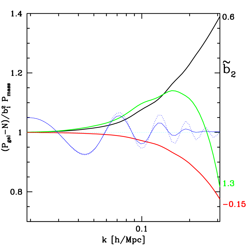
Figure 1: Thick lines show $(P_{g}(k)-N)/b_{1}^{2}P_{\rm mass}(k)$ for $\tilde{b}_{2}=0.6$ (black), $\tilde{b}_{2}=1.3$ (green), and $\tilde{b}_{2}=-0.15$ (red). For comparison, the thinner, blue, wiggly lines show the ratio of mass power in a realistic model to the power in a similar model with no baryonic acoustic oscillations (solid is non-linear power, dotted is linear).

The cosmological model for this figure, plotted at $z=0$, was flat with $\sigma_{8}=0.85$, $n=0.96$, $\Omega_{m}=0.281$, $h=0.71$, and $\Omega_{b}=0.0462$ (Seljak et al., 2006), with CMBfast (Seljak and Zaldarriaga, 1996) used to generate the transfer function. We see the desired convergence to the simple linear bias plus white noise model on large scales. The term $\propto\tilde{b}_{2}^{2}$ is generally negative, while the term $\propto\tilde{b}_{2}$ has the sign of $\tilde{b}_{2}$. This means that when increasing $\tilde{b}_{2}$ from zero we obtain an increase in power at first, up to $\tilde{b}_{2}\simeq 0.6$, but then a decrease, especially at higher $k$, as the $\tilde{b}_{2}^{2}$ term takes over. While this bias term has a maximum, note that the simple ratio of galaxy to mass power does not, because extra white noise power can always be added. For increasingly negative $\tilde{b}_{2}$ both terms are negative so the power decreases quickly (again, noise power can be added, so negative $\tilde{b}_{2}$ does not automatically mean that the bias as traditionally defined decreases). It is interesting to note that there are only hints of features related to baryonic acoustic oscillations (BAO) in the ratio $(P_{g}(k)-N)/b_{1}^{2}P_{\rm mass}(k)$, at the 0.3% level for the $\tilde{b}_{2}=0.6$ case. Combining their small size with the fact that much of the effect appears to be a modification of the amplitude of the wiggles, rather than their position, suggests that 1% distance measurements using BAO should not be significantly corrupted. Of course, these effects, the effect of broad-band $k$-dependence of the bias, and the modification already present in the non-linear mass power spectrum, should not be ignored when fitting observations.

In Fig. 2 I explore the sensitivity of the higher order bias terms to high-$k$ power.

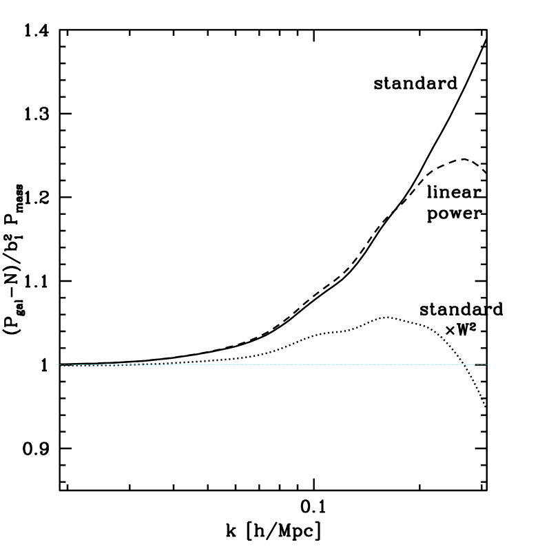
Figure 2: $(P_{g}(k)-N)/b_{1}^{2}P_{\rm mass}(k)$ for $\tilde{b}_{2}=0.6$. The solid curve is my standard calculation, where the RG-corrected (non-linear) mass power spectrum has been used to compute the bias terms. To show the lack of sensitivity to small scales, for the dashed curve the usual linear mass power, which becomes dramatically different from the RG power with increasing $k$, was used to compute the bias terms. The dotted curve shows the effect of a $2\,h^{-1}\,{\rm Mpc}$ rms Gaussian smoothing applied to the result of the standard calculation.

For the standard results I have used the RG-improved power spectrum of McDonald (2006) to compute these terms, but in this figure I compare to the result when I use the standard linear power spectrum. We see that there is not much difference between the results for these cases, even though the RG power is 37% larger at $k=0.3\,h\,{\rm Mpc}^{-1}$, more than a factor of 3 larger at $k=1\,h\,{\rm Mpc}^{-1}$, and the asymptotic slopes at high $k$ are $-1.4$ vs. $\sim-3$. This is a testament to how successful the inoculation against high-$k$ power has been (recall that the unrenormalized bias-related corrections in the RG case would be literally infinite, and some of the corrections using standard PT nearly so). I used $\tilde{b}_{2}=0.6$ for the figure, but the results for larger or smaller $\tilde{b}_{2}$ are similar. An increase in sensitivity to small scale power with increasing $\tilde{b}_{2}$ indicates that the term quadratic in $\tilde{b}_{2}$ is more sensitive than the linear term. For reference, Fig. 2 also shows the effect of Gaussian smoothing with rms width $2\,h^{-1}\,{\rm Mpc}$, which gives $\sigma=1.26$ for the model in the figures, i.e., not really perturbative. The direct power suppression for this smoothing is already substantial, reaching 30% at $k=0.3\,h\,{\rm Mpc}^{-1}$.

II.1 Three-point function

At the order in $\delta_{1}$ considered here, the three-point function (and presumably other similar statistics that require only computation to this order) (Frieman and Gaztanaga, 1994; Scoccimarro et al., 1998; Feldman et al., 2001; Verde et al., 2002; Mandelbaum et al., 2003; Pan and Szapudi, 2005; Hikage et al., 2005; Gaztañaga and Scoccimarro, 2005; Gaztañaga et al., 2005; Ross et al., 2006) is described neatly by the renormalized model, with no non-trivial new effects. In real space it is

$$\left<\delta_{g}(\mathbf{x}_{a})\delta_{g}(\mathbf{x}_{b})\delta_{g}(\mathbf{x}_{c})\right>=\zeta_{g}^{abc} = c_{1}^{3}\left<\delta_{a}\delta_{b}\delta_{c}\right>+\frac{1}{2}c_{1}^{2}c_{2}\left<\delta_{a}\delta_{b}\left(\delta_{c}^{2}-\sigma^{2}\right)+{\rm cyclic~{}permutations}\right>+...$$ (17)

$$= c_{1}^{3}\zeta_{abc}+\frac{1}{2}c_{1}^{2}c_{2}\left(\xi_{ac}\xi_{bc}+{\rm cyclic}\right)+...$$

Since this is already $\mathcal{O}\left(\delta_{1}^{4}\right)$ we can freely substitute $c_{1}\rightarrow b_{1}$ to produce

$$\zeta^{abc}_{g}=b_{1}^{3}\left[\zeta_{abc}+\frac{1}{2}\tilde{b}_{2}\left(\xi_{ac}\xi_{bc}+{\rm cyclic}\right)\right]+...$$ (18)

Deviations from the simplest model are again controlled entirely by $\tilde{b}_{2}$.

III Discussion

The standard method for including biasing of tracers of mass density in perturbation theory calculations of large-scale clustering (Fry and Gaztanaga, 1993; Heavens et al., 1998) uses five parameters to model the power spectrum and bispectrum up to 4th order in density perturbations, and requires at least one arbitrary cutoff parameter (smoothing scale). In the standard approach the effects of the beyond-linear order bias parameters and the cutoff propagate to asymptotically large scales. (Admittedly, this “standard” method has not yet been used much for interpreting data, but this may change soon.) After my redefinitions we have only four parameters, with much more cleanly separated effects:

$${\rm standard~{}parameters} \longrightarrow \rho_{0},~{}\rho_{0}^{\prime},~{}\rho_{0}^{\prime\prime},~{}\rho_{0}^{\prime\prime\prime},~{}N_{0},~{}{\rm and~{}messy~{}cutoffs}$$

$${\rm new~{}parameters} \longrightarrow \bar{\rho}_{g},~{}b_{1},~{}\tilde{b}_{2},~{}{\rm and}~{}N~{}.$$

Heavens et al. (1998) provided the core calculations for this paper. The innovation here is the suggestion that their effective linear bias and shot-noise-like term should not be treated as output predictions of the model but instead should be absorbed into renormalized linear bias and shot-noise parameters. Significantly, these new free parameters of the model contain most of the high-$k$ (small, non-linear scale) sensitivity in the bias calculation. Rather than having a large-scale effective bias (ratio of tracer power to mass power) which is a function of all three bias parameters in the model, and the smoothing scale, I have only a single parameter for the large-scale bias. Rather than shot-noise that is a function of the original stochasticity, the 2nd order bias, and the smoothing scale, I have a single shot-noise parameter that describes all asymptotically large-scale deviation from the linear bias model. Quasi-linear deviation from the linear bias plus shot-noise model is described by a single parameter, with no need for smoothing.

One might ask if it is desirable to bury time and cosmology dependence, in the form of the values of $\sigma^{2}$ and $\int dq~{}q^{2}P(q)^{2}$, in $b_{1}$ and $N$. Do we not lose information this way? The answer is: not really, because $c_{1}$, $c_{2}$, $c_{3}$, and $N_{0}$ are also mixed into $b_{1}$ and $N$, and, even for fixed smoothing scale, generally none of these parameters will be independent of the cosmological model or of time. Furthermore, $\sigma^{2}$ and $\int dq~{}q^{2}P(q)^{2}$ are relatively sensitive to high-$k$ power which is poorly described by perturbation theory.

Note that simulations or other microscopic models of galaxy formation can still be used to calibrate the renormalized large-scale structure model. The way this works exemplifies the usefulness of the revised model. The most straightforward method for calibrating the unrenormalized model is to pick some smoothing scale and measure directly the parameters of the original Taylor series, Eq. (1). If this is done very literally (e.g., by making a scatter plot of galaxy density vs. smoothed mass density and reading off derivatives at $\delta=0$), one is not even guaranteed that the calibrated model will reproduce the mean density of galaxies in the simulations used to calibrate it (without the trivial renormalization of the first term in the Taylor series, discussed above), let alone the large-scale bias, the shot-noise, or really anything else about large-scale structure. (I emphasize here that I am not saying this method will surely fail, only that it is not guaranteed to work.) To calibrate the renormalized model one computes the mean density and power spectrum from the simulation, and if desired the bispectrum, and then fits for the parameters of the model. This guarantees that the large-scale structure in the simulation will be reproduced by the model as well as possible. Of course, one can be less literal and calibrate the unrenormalized model by fitting the simulated statistics, but this still includes the extra steps of choosing a smoothing scale and computing the simple observables (e.g., mean density, large scale bias) as a function of several parameters. Of course, as I discussed above, there is an additional problem with the literal use Eq. (1) in that any smoothing aggressive enough to render the density fluctuations small will also corrupt the power on interesting, perturbative scales.

Within the perturbative approach there is a simulation-independent means of estimating the validity of the results. One can go through the full process of extracting the cosmological parameters of most fundamental interest from the data, marginalizing over the bias parameters, using the perturbative model calculated to two different orders, and compare the results. As presented here, the results from linear theory could be compared to the model with the first non-linear corrections, although computing to another order might be useful in the future (of course, higher order is necessary if one wants to use the bispectrum to two different non-zero orders). The level of agreement would surely depend on the maximum $k$ used in the fit. This maximum $k$ could be chosen small enough to ensure agreement, i.e., consistency of the perturbative model.

There are several obvious next steps for this line of work: Extension to redshift space McDonald (2003); Scoccimarro (2004) should be straightforward, following the calculations of Heavens et al. (1998). A more general time and space-local model could be implemented, e.g., once one goes beyond linear theory the Taylor series for $\rho_{g}$ should probably include velocity divergence terms as well as density terms. As discussed by McDonald (2006), it may be possible to make non-trivial predictions about the time evolution of bias by starting the perturbative calculation from a model for the local formation (and merging, etc.) rate of the tracer (Tegmark and Peebles, 1998; Simon, 2005), rather than the instantaneous density of the tracer (this will probably require a renormalization group approach as in McDonald (2006), rather than simple parameter redefinitions as in this paper). Extension to multiple luminosities or types of galaxies (or more divers tracers Taruya (2000); McDonald et al. (2002); Skibba et al. (2006)) can be done by writing a Taylor series like Eq. (1) for each. This will lead to extra parameters, but cross-correlation will provide extra observables to constrain them.

Finally, I observe that, beyond just removing badly behaved perturbative terms at the present order of calculation, by treating the linear bias and shot-noise as free parameters we are in effect already accounting for similar terms that appear at any order in perturbation theory. This is probably the most compelling reason to believe that the approach of this paper can be expected work better than the standard approach as presented (the problem in the standard approach of smoothing corrupting the power on interesting scales is also significant). It may be possible to show that all higher order corrections to the tracer power as $k\rightarrow 0$ can be included in these two terms, i.e., that the renormalized linear bias and shot-noise give a fundamentally complete descriptions of very large-scale clustering Scherrer and Weinberg (1998).