Selection bias in the $M_{\bullet}-\sigma$ and $M_{\bullet}-L$ correlations and its consequences

Abstract

It is common to estimate black hole abundances by using a measured correlation between black hole mass and another more easily measured observable such as the velocity dispersion or luminosity of the surrounding bulge. The correlation is used to transform the distribution of the observable into an estimate of the distribution of black hole masses. However, different observables provide different estimates: the $M_{\bullet}-\sigma$ relation predicts fewer massive black holes than does the $M_{\bullet}-L$ relation. This is because the $\sigma-L$ relation in black hole samples currently available is inconsistent with that in the SDSS sample, from which the distributions of $L$ or $\sigma$ are based: the black hole samples have smaller $L$ for a given $\sigma$ or have larger $\sigma$ for a given $L$. This is true whether $L$ is estimated in the optical or in the NIR. The $\sigma-L$ relation in the black hole samples is similarly discrepant with that in the ENEAR sample of nearby early-type galaxies. This suggests that current black hole samples are biased towards objects with abnormally large velocity dispersions for their luminosities. If this is a selection rather than physical effect, then the $M_{\bullet}-\sigma$ and $M_{\bullet}-L$ relations currently in the literature are also biased from their true values. We provide a framework for describing the effect of this bias. We then combine it with a model of the bias to make an estimate of the true intrinsic relations. While we do not claim to have understood the source of the bias, our simple model is able to reproduce the observed trends. If we have correctly modeled the selection effect, then our analysis suggests that the bias in the $\langle M_{\bullet}|\sigma\rangle$ relation is likely to be small, whereas the $\langle M_{\bullet}|L\rangle$ relation is biased towards predicting more massive black holes for a given luminosity. In addition, it is likely that the $M_{\bullet}-L$ relation is entirely a consequence of more fundamental relations between $M_{\bullet}$ and $\sigma$, and between $\sigma$ and $L$. The intrinsic relation we find suggests that at fixed luminosity, older galaxies tend to host more massive black holes.

1. Introduction

Several groups have noted that galaxy formation and supermassive black hole growth should be related, and many have modeled the joint evolution of quasars and galaxies (e.g., Monaco et al. 2000; Kauffmann & Haehnelt 2001; Granato et al. 2001; Cavaliere & Vittorini 2002; Cattaneo & Bernardi 2003; Haiman et al. 2004; Hopkins et al. 2004; Lapi et al. 2006; Haiman et al. 2006 and references therein). However, the number of black hole detections to date is less than fifty; this small number prevents a direct estimate of the black hole mass function. On the other hand, correlations between $M_{\bullet}$ and other observables can be measured quite reliably, if one assumes that the $M_{\bullet}-$observable relation is a single power-law. $M_{\bullet}$ is observed to correlate strongly and tightly with the velocity dispersion of the surrounding bulge (Ferrarese & Merritt 2000; Gebhardt et al. 2000; Tremaine et al. 2002), as well as with bulge luminosity (McLure & Dunlop 2002) and bulge stellar mass (Marconi & Hunt 2003; Häring & Rix 2004): in all cases, a single power law appears to be an adequate description.

Since it is considerably easier to measure bulge properties than $M_{\bullet}$, black hole abundances are currently estimated by transforming the observed abundances of such secondary indicators using the observed correlations with $M_{\bullet}$ (Yu & Tremaine 2002; Aller & Richstone 2002; Marconi et al. 2004; Shankar et al. 2004; McLure & Dunlop 2004). Unfortunately, combining the $M_{\bullet}-\sigma$ relation with the observed distribution of velocity dispersions results in an estimate of the number density of black holes with $M_{\bullet}>10^{9}M_{\odot}$ which is considerably smaller than the estimate based on combining the $M_{\bullet}-L$ relation with the observed luminosity function (Tundo et al. 2006).

The fundamental cause of the discrepancy is that the luminosity and velocity dispersion functions are obtained from the SDSS (Blanton et al. 2003; Sheth et al. 2003), but the $\sigma-L$ relation in the SDSS (Bernardi et al. 2003b) is different from that in the black hole samples (e.g. Yu & Tremaine 2002). In Section 2, we argue that the SDSS $\sigma-L$ relation is not to blame, suggesting that it is the black hole samples which are biased.

Figure 1.— Comparison of the $\sigma-L$ relation in the black hole sample of Häring & Rix (2004) (symbols) with that from local early-type galaxy samples (lines). We provide two estimates of the bulge luminosity for the Häring & Rix compilation: the open circles come from rescaling the bulge luminosity to the SDSS r-band, and the filled circles from assuming a mass-to-light ratio to scale the bulge masses $M_{\rm bulge}$ to luminosities. Dotted line shows a fit to the filled circles. Solid and short dashed lines show $\langle\sigma|L\rangle$ in the SDSS-B06 and ENEAR samples. Dot-dashed line shows the biased relation obtained from the ENEAR sample if one fails to account for the fact that the velocity dispersions played an important role in determining the distances from which the luminosities were estimated. The black hole compilation is clearly offset from the SDSS-B06, the ENEAR and even the biased ENEAR relations. Appendix A gives the fits shown, and describes exactly how the black hole sample was compiled.

If black hole samples are indeed biased, then this bias may be physical or it may simply be a selection effect. If physical, then only a special set of galaxies host black holes, and the entire approach above (of transforming the luminosity or velocity dispersion function) is compromised. On the other hand, if it is a selection effect, then one is led to ask if the $M_{\bullet}-$observable relations currently in the literature are biased by this selection or not. The main purpose of this work is to provide a framework for describing these biases. Section 3 describes Monte-Carlo simulations of the selection effect. It shows an example of the bias which results, and provides an analytic model of the effect. Our findings are summarized in Section 4, where estimates of the intrinsic black hole mass function $\phi(M_{\bullet})$, and the intrinsic $M_{\bullet}-\sigma$ and $M_{\bullet}-L$ relations are provided.

Throughout, we assume a spatially flat background cosmology with $\Omega_{0}=0.3$ and a cosmological constant. All luminosities and masses have been scaled to $H_{0}=70$ km s^-1 Mpc^-1.

2. Motivation: The $\sigma-L$ relation

This section shows that the $\sigma-L$ relation of early-type galaxies is significantly different from that in current black hole samples. This difference exists whether $L$ is computed in a visual band, or in the near-infrared.

2.1. Remarks on SDSS photometry and spectroscopy

Since 2002, when the Bernardi et al. (2003a) sample was compiled, a number of systematic problems with SDSS photometry and spectroscopy have been discovered. The initial (SDSS-DR1 and earlier) photometry overestimated the luminosities and sizes of extended objects. Although later releases correct for these problems, they still overestimate the sky level in crowded fields (e.g. Mandelbaum et al. 2005; Bernardi et al. 2006; Lauer et al. 2006), and so they tend to underestimate the luminosities of extended objects in such fields. This problem is particularly severe for early-type galaxies in nearby clusters. In addition, the SDSS slightly overestimates the velocity dispersions at small $\sigma$ (the velocity dispersions in Bernardi et al. 2003a differ from the values reported in the SDSS database and are not biased at small $\sigma$). Bernardi (2006) discusses an analysis of the $\sigma-L$ which results once all these systematic effects have been corrected-for: the net effect does not significantly change the $\sigma-L$ relation reported by Bernardi et al. (2003b). Nevertheless, the results which follow are based on luminosities and velocity dispersions which have been corrected for all these effects. Because they are not easily obtained from the SDSS database, in what follows, we refer to the corrected SDSS sample as the SDSS-B06 sample.

Bernardi (2006) shows that the $\sigma-L$ relation in the SDSS-B06 sample is consistent with that in ENEAR, the definitive sample of nearby (within 7000 km s^-1) early-type galaxies (da Costa et al. 2000; Bernardi et al. 2002; Alonso et al. 2003; Wegner et al. 2003), provided that one accounts for the bias which arises from the fact that $\sigma$ played an important role in determining $L$. Hence, the local (ENEAR) and not so local determinations (SDSS-B06) of the $\sigma-L$ relation are consistent with one another.

2.2. The $\sigma-L$ relations in the optical

Figure 1 compares the correlation between $\sigma$ and $L$ in ENEAR and SDSS-B06 with that in the recent compilations of black holes by Häring & Rix (2004). The dotted line shows a fit to $\langle\sigma|L\rangle$ defined by the filled circles. Appendix A describes this and other black hole compilations we have consider in the following figures. It also gives the fits shown in this and the other figures.

The solid line shows $\langle\sigma|L\rangle$ in the SDSS-B06 sample. The dot-dashed line shows a determination of the ENEAR $\sigma-L$ relation which attempts to correct for peculiar velocity effects in the distance estimate. This correction is known to bias the $\langle\sigma|L\rangle$ relation towards a steeper slope (Bernardi 2006). The short-dashed line shows the result of using the redshift as distance indicator when computing the ENEAR luminosities; while not ideal, comparison of this relation with the dot-dashed line provides some indication of the magnitude of the bias. Note in particular that using the redshift as distance indicator brings the ENEAR relation substantially closer to the SDSS-B06 relation, for which the redshift is an excellent distance indicator.

The agreement between ENEAR and SDSS-B06 suggests that the difference between the $\sigma-L$ relation in the black hole sample (dotted) and in SDSS-B06 (solid) cannot be attributed to problems with the SDSS determination.

The agreement between ENEAR and SDSS-B06, and the disagreement with the black hole samples strongly suggests that the $\sigma-L$ relation in black hole samples is biased to larger $\sigma$ for given $L$, or to smaller $L$ for a given $\sigma$. Similar conclusions are obtained if we use Kormendy & Gebhardt (2001) or Ferrarese & Ford (2005) compilations. At a given luminosity, the black hole samples have $\log\sigma$ larger than the ENEAR or SDSS-B06 relations by $\sim 0.1$ dex. As a result of this difference, smaller luminosities can apparently produce black holes of larger mass than do their associated velocity dispersions (e.g., Yu & Tremaine 2002). Tundo et al. (2006) show this in some detail.

2.3. The $\sigma-L$ relations in the near-infrared

We have considered the possibility that the discrepancy between the $\sigma-L$ relations may depend on wavelength. Figure 2 presents a similar analysis, but now the luminosities are from the $K$-band. In the case of the early-type sample, the SDSS-B06 sample was matched to 2MASS, and then the 2MASS isophotal magnitudes were brightened by 0.2 mags to make them more like total magnitudes (Kochanek et al. 2001; Marconi & Hunt 2003). The solid line shows the resulting $\langle\sigma|L_{\rm K}\rangle$ relation. It is very similar to that in the $r-$band if $r-K=2.8$.

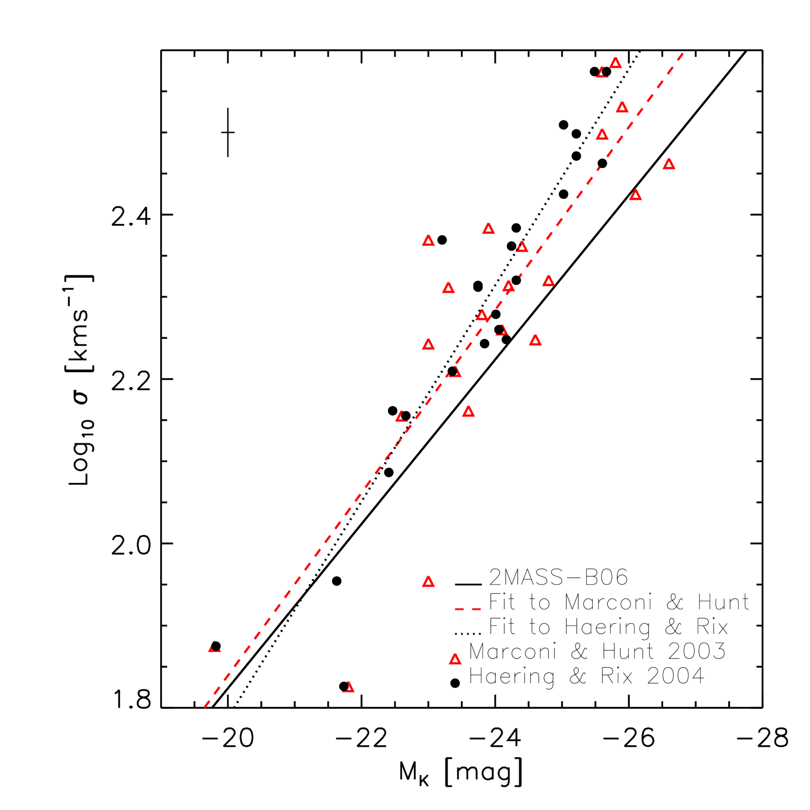
Figure 2.— Same as Figure 1 but now using the $K$-band luminosity. Triangles show the subset of the Häring & Rix sample for which $K$-band luminosity estimates are available (from Marconi & Hunt 2003). Solid circles show the result of rescaling the $M_{\rm bulge}$-based luminosities of these objects to the $K$-band using $r-K=2.8$. Dotted and dashed lines show fits to the $\langle\sigma|L_{\rm K}\rangle$ relations defined by these points. Solid line shows $\langle\sigma|L_{\rm K}\rangle$ obtained by matching the SDSS-B06 early-type sample to the 2MASS database, and then using the $K$-band luminosities with the SDSS-B06 velocity dispersions. This fit is very similar to the solid line shown in the previous panels if $r-K=2.8$. These fits are given in Appendix A.

Marconi & Hunt (2003) matched their black hole compilation to 2MASS, and then recomputed the photometry to determine $L_{\rm K}$. The open triangles show the $\sigma-L_{\rm K}$ relation for the subset of objects which are in the Häring & Rix sample. The filled circles are obtained by taking these objects (i.e. those in both Marconi & Hunt and Häring & Rix), and then shifting the $M_{\rm bulge}$ based $r-$band luminosities to $K$ assuming $r-K=2.8$. Dashed and dotted lines show fits to these relations. Comparison with the solid line (2MASS-B06) shows a significant offset—the black hole samples are different from the population of normal early-type galaxies.

3. Biases in the $M_{\bullet}-\sigma$ and $M_{\bullet}-L$ relations

If black hole samples are indeed biased, then this bias may be physical or simply a selection effect. One is then led to ask if the relations currently in the literature are biased by this selection or not. To address this, we must be able to quantify how much of the $M_{\bullet}-\sigma$ correlation arises from the $M_{\bullet}-L$ and $L-\sigma$ relations, and similarly for the $M_{\bullet}-L$ relation.

3.1. Demonstration using mock catalogs

Our approach is to make a model for the true joint distribution of $M_{\bullet}$, $L$ and $\sigma$, and to study the effects of selection by measuring the various pairwise correlations before and after applying the selection procedure to this joint distribution. In what follows, we will use $V=\log\,(\sigma/{\rm km~{}s}^{-1})$, and with some abuse of notation, $M_{\bullet}$ to denote the logarithm of the black hole mass when expressed in units of $M_{\odot}$ and $L$ to denote the absolute magnitude (since, in the current context, $M$ for absolute magnitude is too easily confused with mass). We assume that correlations between the logarithms of these quantities define simple linear relations, so our model has nine free parameters: these may be thought of as the slope, zero-point and scatter of each of the three pairwise correlations, or as the means and variances of $L$, $V$ and $M_{\bullet}$ and the three correlation coefficients $r_{VL}$, $r_{\bullet V}$ and $r_{\bullet L}$.

To illustrate, let $\langle V\rangle$ and $\sigma_{V}$ denote the mean and rms values of $V$, and use similar notation for the other two variables. Then the mean $V$ as a function of $L$ satisfies

$${\langle V|L\rangle-\langle V\rangle\over\sigma_{V}}={L-\langle L\rangle\over\sigma_{L}}\ r_{VL},$$ (1)

and the rms scatter around this relation is

$$\sigma_{V|L}=\sigma_{V}\,\sqrt{1-r_{VL}^{2}}.$$ (2)

The combination $a_{V|L}\equiv r_{VL}\,\sigma_{V}/\sigma_{L}$ is sometimes called the slope of the $\langle V|L\rangle$ relation, and $\langle V\rangle-a_{V|L}\,\langle L\rangle$ is the zero-point. Similarly, the slopes of $\langle M_{\bullet}|V\rangle$ and $\langle M_{\bullet}|L\rangle$ are $a_{\bullet|V}\equiv r_{\bullet V}\,\sigma_{\bullet}/\sigma_{V}$ and $a_{\bullet|L}\equiv r_{\bullet L}\,\sigma_{\bullet}/\sigma_{L}$ respectively. Notice that the zero points are trivial if one works with quantities from which the mean value has been subtracted. We will do so unless otherwise specified.

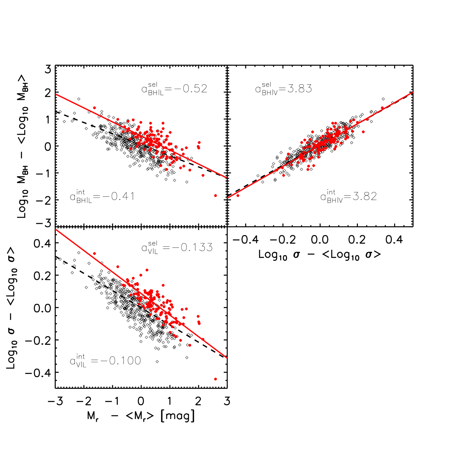
Figure 3.— Comparison of the joint distribution of $M_{\bullet}$, $\sigma$ and $L$, before (open symbols) and after (filled symbols) applying a selection cut. Dashed and solid lines show the intrinsic and observed correlations. The probability of selection is assumed to increase as one moves to the right of the dashed line in the bottom left panel.

Our analysis is simplified by the fact that five of the nine free parameters are known: the mean and rms values of $L$ and $V$ as well as the correlation between $V$ and $L$ have been derived from the SDSS-B06 sample (these values are similar to those reported by Bernardi et al. 2003b, who also show that the distribution of $V$ given $L$ is Gaussian). Hence, we use

$$\sigma_{L}=0.84,\quad\sigma_{V}=0.11,\quad{\rm and}\quad r_{VL}=-0.78,$$

to make a mock catalog of the joint $V-L$ distribution in the SDSS-B06 early-type galaxy sample. Sheth et al. (2003) show explicitly that the resulting mock catalog provides luminosity and velocity dispersion functions which are consistent with those seen in the SDSS.

We turn this into a catalog of black hole masses by assuming that, like $V$ at fixed $L$, the distribution of $M_{\bullet}$ at fixed $V$ and $L$ is Gaussian. Hence, for each $V$ and $L$, we generate a value of $M_{\bullet}$ that is drawn from a Gaussian distribution with mean

$${\langle M_{\bullet}|L,V\rangle\over\sigma_{\bullet}} = {\langle M_{\bullet}\rangle\over\sigma_{\bullet}}+{L-\langle L\rangle\over\sigma_{L}}\,{r_{\bullet L}-r_{\bullet V}r_{VL}\over 1-r_{VL}^{2}}$$ (3)

$$\quad+\quad{V-\langle V\rangle\over\sigma_{V}}\,{r_{\bullet V}-r_{\bullet L}r_{VL}\over 1-r_{VL}^{2}},$$

and rms

$$\sigma_{\bullet|LV}=\sigma_{\bullet}\,\sqrt{1-r_{VL}^{2}-r_{\bullet V}^{2}-r_{\bullet L}^{2}+2r_{VL}r_{\bullet L}r_{\bullet V}\over 1-r_{VL}^{2}}$$ (4)

(see, e.g., Bernardi et al. 2003b). The combination $r_{\bullet V}r_{VL}$ measures how much of the correlation between $M_{\bullet}$ and $L$ is simply a consequence of the correlations between $M_{\bullet}$ and $V$ and between $V$ and $L$. The combination $r_{\bullet L}r_{VL}$ can be interpreted similarly. Notice again that the mean values of the three quantities mainly serve to set the zero-points of the correlations. Since we are working with quantities from which the mean has been subtracted, our model for the true relations is fixed by specifying the values of $\sigma_{\bullet}$, $r_{\bullet V}$ and $r_{\bullet L}$.

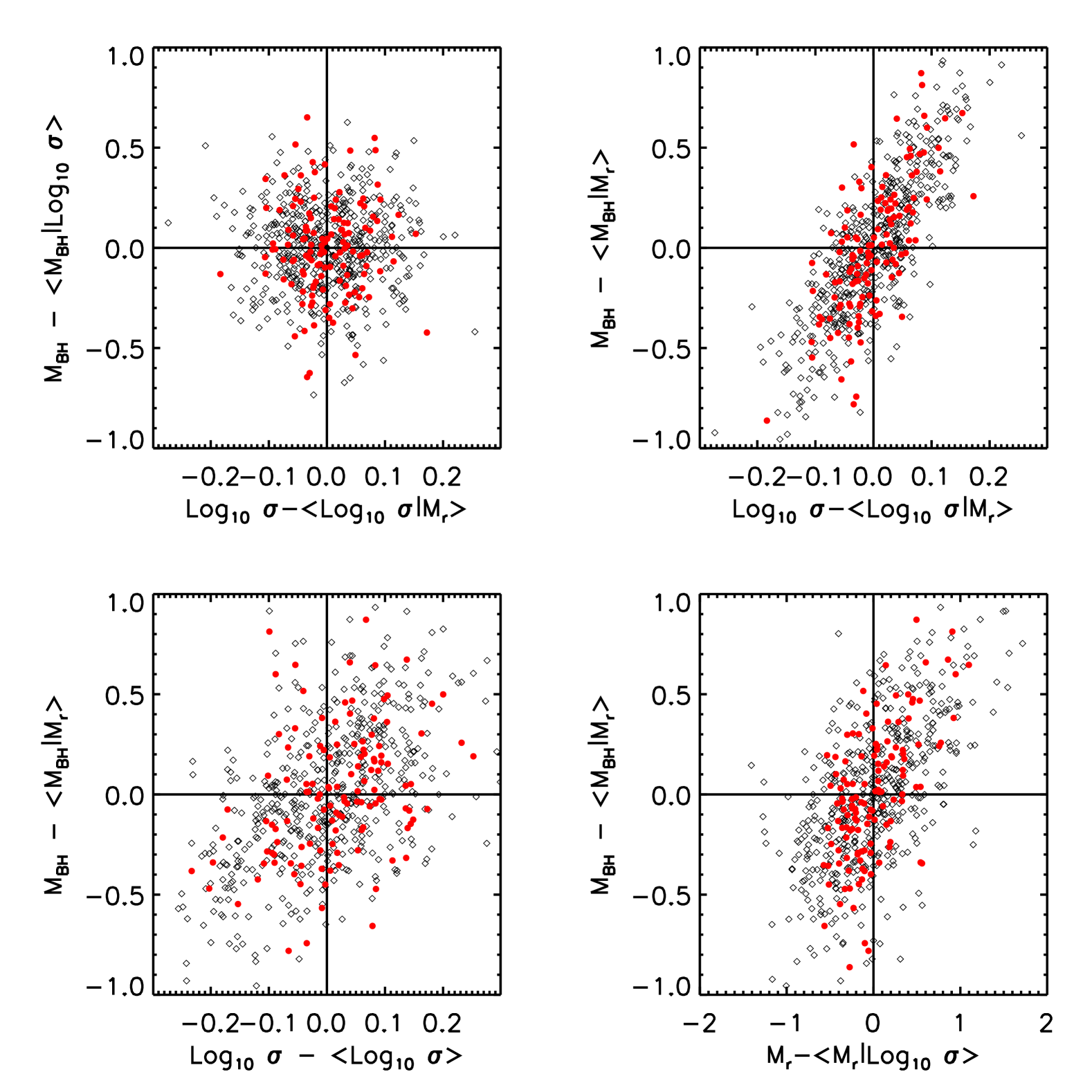
Figure 4.— Residuals from the $M_{\bullet}-\sigma$ relation do not correlate with residuals from the $\sigma-L$ correlation (top left); whereas residuals from the $M_{\bullet}-L$ relation do (top right). They also correlate with residuals from the $L-\sigma$ relation (bottom right), and weakly with $\sigma$ (bottom left). In all panels, open circles show the intrinsic correlations and filled circles show correlations after applying the selection cut. Comparison with Figure 7 shows that the filled circles trace similar locii to those seen in the Häring & Rix (2004) compilation.

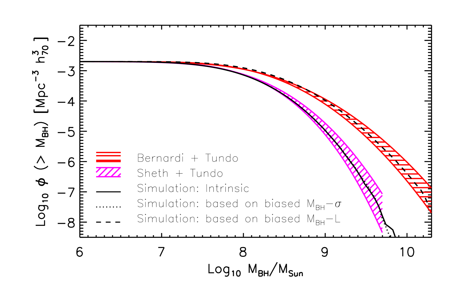
Figure 5.— Comparison of the intrinsic (solid) and selection-biased counts based on using velocity dispersion (dotted) and luminosity (dashed) as the indicator of $M_{\bullet}$. Hashed regions show the abundances infered by Tundo et al. (2006) by combining the $M_{\bullet}-L$ and $M_{\bullet}-\sigma$ relations in the compilation of Häring & Rix (2004) with the SDSS-based luminosity and velocity functions (Bernardi et al. 2003b; Sheth et al. 2003).

To study how selection effects might have biased the observed $M_{\bullet}-\sigma$ and $M_{\bullet}-L$ relations we generate a mock galaxy+black hole catalog as described above, model the selection effect, and then measure the three pairwise correlations in the selection-biased catalog. Figure 3 shows an example of the result when

$$\sigma_{\bullet}=0.49,\quad r_{\bullet V}=0.88,\quad{\rm and}\quad r_{\bullet L}=-0.70.$$

We have tried a variety of ways to specify a selection effect. In Figure 3, we supposed that no objects with luminosities brighter than $\langle L|V\rangle$ were selected, and that the fraction of fainter objects which are selected is ${\rm erf}(x/\sqrt{2})$, where $x=(L-\langle L|V\rangle)/\sigma_{L|V}$. The open diamonds in each panel show the objects in the original catalog, and the filled circles show the objects which survived the selection procedure. The panels also show the slopes of the relations before (dashed) and after (solid) selection. Note that because the selection was made at fixed $V$, the slope of $\langle M_{\bullet}|V\rangle$ in the selected sample is not changed from its original value. However, $\langle M_{\bullet}|L\rangle$ and $\langle V|L\rangle$ are both steeper than before. The exact values of the change in slope depend upon our choices for the intrinsic model, for reasons we describe in the next subsection.

The parameter choices given above, with the selection described above, result in zero-points, slopes (given at top of each panel) and scatter (0.22 dex, 0.33 dex and 0.05 dex in the top left, right, and bottom panels, respectively) which are in excellent agreement with those in the Häring & Rix (2004) compilation (see Appendix A). Figure 4 shows that residuals from these relations exhibit similar correlations to those seen in the real data (compare Figure 7; residuals from the $M_{\bullet}-\sigma$ relation do not correlate with $\sigma$, $L$ or $L-\sigma$ residuals, so we have not shown these correlations here). This agreement is nontrivial: for example, it is more difficult to match all three observed correlations if the selection is based on $\langle V|L\rangle$ rather than $\langle L|V\rangle$. Changes in the parameter values of more than five percent produce noticable differences.

The correlations shown in the two right hand panels of Figure 4 are similar in the full and in the bias selected sample, suggesting that the selection has not altered the shape of this correlation. This suggests that the correlations seen in the right hand panel of Figure 7 are real–they are not due to selection effects. We comment in the final section on what these correlations might imply.

The result of using the biased $\langle M_{\bullet}|L\rangle$ relation (both slope and scatter) in the mock luminosity function to predict black hole abundances is shown as the dashed line in Figure 5. It overpredicts the true abundances in the mock catalog, which are shown by the solid line. The dotted line shows that the analogous $\sigma-$based predictor is, essentially unbiased. This is not surprising in view of the results shown in Figure 3—the observed $\langle M_{\bullet}|L\rangle$ relation is biased towards predicting more massive black holes for a given luminosity, whereas the $\langle M_{\bullet}|\sigma\rangle$ is almost completely unbiased. The hashed regions show the $L-$ and $\sigma-$based predictions derived by using the relations in the Appendix (taken from Tundo et al. 2006) with the Bernardi et al. (2003b) luminosity function and the Sheth et al. (2003) velocity function. They bracket the results from our mock catalog quite accurately. Note, however, that in our mock catalog, the true abundances are given by the solid line: the much larger abundances predicted from the luminosity-based approach are due to the selection effect. For reference, this intrinsic distribution is well-described by equation (8).

3.2. Toy model of the bias

If current black hole samples only select objects which have $\log\sigma$ which is exactly $n$-standard deviations above the $\langle V|L\rangle$ relation, then

$${V-\langle V\rangle\over\sigma_{V}}={L-\langle L\rangle\over\sigma_{L}}\ r_{VL}+n\,\sqrt{1-r_{VL}^{2}},$$ (5)

and inserting this in the expression above yields

$${\langle M_{\bullet}|L\rangle\over\sigma_{\bullet}}={\langle M_{\bullet}\rangle\over\sigma_{\bullet}}+n\,{r_{\bullet V}-r_{\bullet L}r_{VL}\over\sqrt{1-r_{VL}^{2}}}+{L-\langle L\rangle\over\sigma_{L}}\,r_{\bullet L}.$$ (6)

The slope of this relation is still $a_{\bullet|L}$; because the selection was done at fixed $L$, the slope of the observed $\langle M_{\bullet}|L\rangle$ relation is not biased from its true value. However, the zero-point may be strongly affected. The magnitude of the offset depends on how much of the $M_{\bullet}-\sigma$ relation is due to the $\sigma-L$ and $M_{\bullet}-L$ relations. If $n$ is positive (as Figure 1 suggests) and $r_{\bullet V}>r_{\bullet L}r_{VL}$, then the observed relation predicts larger black hole masses for a given luminosity than would the true relation. The associated $\langle M_{\bullet}|\sigma\rangle$ relation is obtained by transforming $L$ to $V$ using equation (5):

$${\langle M_{\bullet}|V\rangle\over\sigma_{\bullet}} = {\langle M_{\bullet}\rangle\over\sigma_{\bullet}}+{V-\langle V\rangle\over\sigma_{V}}\,r_{\bullet V}\,\left({r_{\bullet L}\over r_{\bullet V}r_{VL}}\right)$$ (7)

$$+n\,r_{\bullet V}\,{1-(r_{\bullet L}/r_{\bullet V}r_{VL})\over\sqrt{1-r_{VL}^{2}}}.$$

Both the slope and zero-point of this relation are affected, and the magnitude of the effect depends on whether or not $r_{\bullet L}>r_{\bullet V}r_{VL}$. If the correlation between $M_{\bullet}$ and $L$ is stronger(weaker) than can be accounted for by the $M_{\bullet}-V$ and $V-L$ relations, then the observed $\langle M_{\bullet}|V\rangle$ has a steeper (shallower) slope than the true relation, and a shifted zero-point, such that it predicts smaller (larger) masses for a given $\sigma$ than the true relation. Note that this means it is possible for both the $L-$ and $\sigma-$based approaches to overestimate the true abundance of massive black holes.

If the selection chooses objects with small $L$ for their $\sigma$, then the resulting relations are given by exchanging $L$s for $V$s in the previous two expressions. In this case, $\langle V|L\rangle$ and $\langle M_{\bullet}|L\rangle$ both have biased slopes and zero points, whereas $\langle M_{\bullet}|\sigma\rangle$ has the correct slope but a shifted zero-point. Once again, the sign and magnitude of the bias depends on how much of the $M_{\bullet}-$observable correlation is due to the other two correlations. For the choice of parameters used to make the Figures in the previous subsection, $r_{\bullet V}r_{VL}=0.69\approx r_{\bullet L}$: the $M_{\bullet}-L$ relation is almost entirely a consequence of the other two correlations. Thus, this toy model shows why the $\langle M_{\bullet}|\sigma\rangle$ relation shown in Figure 3 was unbiased by the selection (which was done at fixed $\sigma$).

4. Discussion

Compared to the ENEAR and SDSS-B06 early-type galaxy samples, the $\sigma-L$ correlation in black hole samples currently available is biased towards large $\sigma$ for a given $L$ (Figures 1–2). If this is a selection effect rather than a physical one, then current determinations of the $M_{\bullet}-L$ and $M_{\bullet}-\sigma$ relations are biased. We provided a simple toy model of the effect which shows how these biases depend on the intrinsic correlations and on the selection effect.

To illustrate its use, we constructed simple models of the intrinsic correlation and of the selection effect. We then identified a particular set of parameters which we showed can reproduce all the observed trends: the correlations between $M_{\bullet}$ and $L$ or $\sigma$, the $\sigma-L$ correlation in black hole samples, as well as correlations between residuals from these fits (Figures 3 and 4) are all reproduced. We do not claim to have found the unique solution to this problem. However, if we have correctly modeled the selection effect, then our analysis suggests that the bias in the $\langle M_{\bullet}|\sigma\rangle$ relation is likely to be small, whereas the $\langle M_{\bullet}|L\rangle$ relation is biased towards having a steeper slope (Figure 3). This has the important consequence that estimates of black hole abundances which combine the $\langle M_{\bullet}|L\rangle$ relation and its scatter with an external determination of the distribution of $L$ will overpredict the true abundances of massive black holes. The analogous approach based on $\sigma$ is much less biased (Figure 5).

The choice of parameters which reproduces the selection-biased fits reported in Appendix A has intrinsic distribution $\phi(M_{\bullet})$ that is well described

$$\phi(M_{\bullet})\,{\rm d}M_{\bullet}={\phi_{*}\over\Gamma(\alpha/\beta)}\,\mu^{\alpha}\,\exp(-\mu^{\beta})\,\beta\,{{\rm d}M_{\bullet}\over M_{\bullet}}$$ (8)

where $\phi_{*}=0.002/{\rm Mpc}^{3}$, $(\alpha,\beta)=(2.0,0.3)$ and $\mu=M_{\bullet}/M_{\bullet}^{*}$, with $M_{\bullet}^{*}$ a characteristic mass. This mass is related to the mean mass $10^{8}M_{\odot}$ by $\langle M_{\bullet}\rangle=M_{\bullet}^{*}\,\Gamma[(\alpha+1)/\beta]/\Gamma(\alpha/\beta)$, so $M_{\bullet}^{*}=10^{5}\,M_{\odot}$. Since this $\phi(M_{\bullet})$ is based on the SDSS-B06 luminosity and velocity functions, it is missing small bulges, so it is incomplete at small $M_{\bullet}$.

The intrinsic correlations in the sample are

$$\Bigl{\langle}M_{\bullet}|M_{r}\Bigr{\rangle}=9.16-0.41\,(M_{r}+22)\\$$ (9)

and

$$\Bigl{\langle}M_{\bullet}|\log\sigma\Bigr{\rangle}=8.85+3.82\,\log\,(\sigma/200~{}{\rm km~{}s}^{-1})$$ (10)

with scatter of 0.38 and 0.23 dex, respectively. A bisector fit to the $M_{\bullet}-L$ relation would have slope $(\sigma_{\bullet}/\sigma_{L})(r_{\bullet L}+1/r_{\bullet L})/2=-0.62$; a similar fit to the $M_{\bullet}-V$ relation would have slope $(\sigma_{\bullet}/\sigma_{V})(r_{\bullet V}+1/r_{\bullet V})/2=4.49$. Notice that the slopes satisfy $a_{\bullet|L}\approx a_{\bullet|V}\,a_{V|L}$. This is because, for this choice of parameters, the correlation between $M_{\bullet}$ and $L$ is almost entirely a consequence of the other two correlations.

If we have correctly modelled the selection effect, and we do not claim to have done so, then our analysis suggests that the intrinsic joint distribution of $M_{\bullet}$, luminosity and $\sigma$ is similar to that between color, luminosity and $\sigma$: of the three pairwise correlations, the two correlations involving $\sigma$ are fundamental, whereas the third is not (Bernardi et al. 2005). Since residuals from the $\langle\sigma|L\rangle$ relation are correlated with age (Bernardi et al. 2005), the correlations shown in the top right panels of Figures 4 and 7 suggest that, at fixed luminosity, older galaxies tend to host more massive black holes than less massive galaxies. Understanding why this is true may provide important insight into black hole formation and evolution.

Appendix A The $\sigma-L$ correlation

The main text compares the $\sigma-L$ relation for the bulk of the early-type galaxy population with that for the black hole sample. This was done by using luminosities transformed to the SDSS $r-$band and scaled to $H_{0}=70$ km s^-1 Mpc^-1. Specifically, we convert from B, V, R, I and K-band luminosities to SDSS $r-$band using

$$B-r=1.25,\quad V-r=0.34\quad r-R=0.27,\quad r-I=1.07,\quad{\rm and}\quad r-K=2.8;$$

these come from Fukugita et al. (1995) for S0s and Es. We describe the samples and required transformations below.

Table 1Parameters of the black hole sample used in this work. HR=Häring & Rix (2004); MH = Marconi & Hunt (2003).
$M_{r}^{\rm HR}$ is from observed absolute magnitude; $M_{r}^{\rm HR-M_{bulge}}$ is inferred from $M_{r}^{\rm HR}-M_{\rm bulge}$ relation.

name	$\sigma^{\rm HR}$	Log10 M${}_{\bullet}^{\rm HR}$	$M_{r}^{\rm HR}$	$M_{r}^{\rm HR-M_{bulge}}$	$\sigma^{\rm MH}$	$M_{K}^{\rm MH}$
	[km s${}^{-1}]$	[MSun]	[mag]	[mag]	[km s${}^{-1}]$	[mag]
M87	375	9.54	$-$23.08	$-$22.86	375	$-$25.60
NGC3379	206	8.06	$-$20.85	$-$20.94	206	$-$24.20
NGC4374	296	8.69	$-$22.22	$-$22.41	$--$	$--$
NGC4261	315	8.77	$-$21.90	$-$22.41	315	$-$25.60
NGC6251	290	8.78	$-$22.69	$-$22.80	290	$-$26.60
NGC7052	266	8.58	$-$22.57	$-$22.22	266	$-$26.10
NGC4742	90	7.20	$-$19.75	$-$18.83	90	$-$23.00
NGC0821	209	7.63	$-$21.43	$-$21.51	209	$-$24.80
IC1459	323	9.46	$-$22.37	$-$22.22	340	$-$25.90
M32	75	6.46	$-$16.99	$-$17.02	75	$-$19.80
NGC2778	175	7.20	$-$20.74	$-$21.04	175	$-$23.00
NGC3115	230	9.06	$-$21.12	$-$21.44	230	$-$24.40
NGC3245	205	8.38	$-$20.85	$-$20.94	205	$-$23.30
NGC3377	145	8.06	$-$20.06	$-$19.67	145	$-$23.60
NGC3384	143	7.26	$-$20.17	$-$19.86	143	$-$22.60
NGC3608	182	8.34	$-$21.24	$-$21.26	182	$-$24.10
NGC4291	242	8.55	$-$21.24	$-$21.51	242	$-$23.90
NGC4473	190	8.10	$-$21.18	$-$21.21	190	$-$23.80
NGC4564	162	7.81	$-$20.31	$-$20.56	162	$-$23.40
NGC4649	375	9.36	$-$22.50	$-$22.69	385	$-$25.80
NGC4697	177	8.29	$-$21.44	$-$21.37	177	$-$24.60
NGC5845	234	8.44	$-$20.11	$-$20.41	234	$-$23.00
NGC7332	122	7.17	$-$20.28	$-$19.61	$--$	$--$
NGC7457	67	6.60	$-$18.85	$-$18.94	67	$-$21.80

Figure 6.— The $M_{\bullet}-L$ and $M_{\bullet}-\sigma$ relations in the subset of the Häring & Rix (2004) sample which we describe in the main text. Solid lines show the fits to the filled circles given in equations (A2) and (A3).

Figure 7.— Residuals from the $M_{\bullet}-\sigma$ relation do not correlate with residuals from the $\sigma-L$ correlation (top left); whereas residuals from the $M_{\bullet}-L$ relation do (top right). Residuals from the $M_{\bullet}-L$ relation also correlate with residuals from the $L-\sigma$ relation (bottom right), but they correlate weakly if at all with $\sigma$ (bottom left).

A.1. The black hole sample

The main properties of the black hole sample shown in Figure 1 are listed in Table 1. The sample was compiled as follows. We selected all objects classified as E or S0 by Häring & Rix (2004) in their compilation of black holes. We excluded NGC 4342 as they recommend, as well as NGC 1023 which Ferrarese & Ford (2005) say should be excluded because it is not sufficiently well resolved. Häring & Rix provide estimates of the bulge luminosities and masses of these objects; these assume $H_{0}=70$ km s^-1 Mpc^-1. For consistency we also rescaled the black hole masses from $H_{0}=80$ km s^-1 Mpc^-1 to $H_{0}=70$ km s^-1 Mpc^-1. We convert from the V, R and I-band luminosities the report to SDSS $r$ using the transformations given above. We use the bulge masses to provide an alternative estimate of the bulge luminosities by setting

$$M_{r}=-22.34-{\log_{10}(M_{\rm bulge}/M_{\odot})-11.52\over 0.492};$$ (A1)

this was obtained from a linear regression of $M_{r}$ on $M_{\rm bulge}$. Table 1 also lists estimates of the K-band near-infrared luminosity from Marconi & Hunt (2003) which are shown in Figure 2.

A word on the velocity dispersions is necessary. Häring & Rix (2004) and Marconi & Hunt (2003) use the velocity dispersions provided by Kormendy & Gebhardt (2001) (two galaxies in Marconi & Hunt have a different value). The two estimates correspond to different apertures ($r_{e}$ and central, which probably means $r_{e}/8$). Tremaine et al. (2002) provide a detailed discussion of aperture effects. However, it is not clear that their assumptions about the scale dependence of the stellar velocity dispersion are consistent with more recent measurements (Cappellari et al. 2006). Since the difference in aperture is not sufficient to account for the discrepancy between black hole samples and the normal early-type galaxy samples we have not made any correction for this difference.

The $M_{\bullet}-L$, $M_{\bullet}-\sigma$, and $\sigma-L$ correlations in the Häring & Rix (2004) sample, with luminosities estimated from $M_{\rm bulge}$ are

$$\Bigl{\langle}\log M_{\bullet}|M_{r}\Bigr{\rangle}=(8.57\pm 0.10)-{(1.30\pm 0.10)\over 2.5}\,(M_{r}+22)$$ (A2)

with scatter of 0.33 dex,

$$\Bigl{\langle}\log M_{\bullet}|\log\sigma\Bigr{\rangle}=(8.21\pm 0.05)+(3.83\pm 0.10)\,\log\left({\sigma\over 200\,{\rm kms}^{-1}}\right)$$ (A3)

with intrinsic scatter of 0.22 dex, and

$$\Bigl{\langle}\log\sigma|M_{r}\Bigr{\rangle}=(2.41\pm 0.10)-{(0.34\pm 0.03)\over 2.5}\,(M_{r}+22)$$ (A4)

(Tundo et al. 2006). Figure 6 shows the $M_{\bullet}-L$ and $M_{\bullet}-\sigma$ relations and these fits. The dotted line in Figure 1 of the main text shows equation (A4).

Figure 7 shows that residuals from the $M_{\bullet}-\sigma$ relation do not correlate with residuals from the $\sigma-L$ correlation (top left), whereas residuals from the $M_{\bullet}-L$ relation do (top right). Residuals from the $M_{\bullet}-\sigma$ relation do not correlate with $\sigma$, $L$ or $L-\sigma$ residuals, so we have not shown these correlations here. However, residuals from the $M_{\bullet}-L$ relation do correlate with residuals from the $L-\sigma$ relation (bottom right) and they may also correlate weakly with $\sigma$ itself (bottom left).

The top right panel suggests that, at fixed luminosity, objects with larger $M_{\bullet}$ tend to have larger $\sigma$. The bottom right panel suggests that these objects also tend to be faint for their $\sigma$. But whether or not these are entirely selection effects is unclear; this is because the relations (A2)–(A4) are a combination of an intrinsic correlation and a selection bias, so that correlations between residuals are also combinations of true and selection-biased relations.

A.2. Fits to early-type galaxy samples

The velocity dispersions for the early-type galaxy population were scaled from their measured values to those they are expected to have within a circular aperture of radius $r_{e}/8$. For ENEAR, when the observed redshift is used as the distance indicator (i.e. no correction is made for peculiar velocities),

$$\Bigl{\langle}\log\sigma|M_{r}\Bigr{\rangle}=(2.300\pm 0.110)-{(0.255\pm 0.018)\over 2.5}\,(M_{r}+22).$$ (A5)

Correcting for peculiar velocities leads to a biased relation, because the correction makes $L$ depend on $\sigma$. This biased relation is

$$\Bigl{\langle}\log\sigma|M_{r}\Bigr{\rangle}=(2.316\pm 0.100)-{(0.318\pm 0.011)\over 2.5}\,(M_{r}+22).$$ (A6)

The galaxies in the SDSS-B06 are sufficiently distant that the SDSS-B06 $\sigma-L$ relation is not affected by peculiar velocities. It is

$$\Bigl{\langle}\log\sigma|M_{r}\Bigr{\rangle}=(2.290\pm 0.080)-{(0.250\pm 0.007)\over 2.5}\,(M_{r}+22).$$ (A7)

Expressions (A5)—(A7) are shown in Figure 1 of the main text. They are taken from Bernardi (2006), where a discussion of the systematics in the magnitudes and velocity dispersion in the SDSS database can be found.

A.3. Analogous quantities in the K-band

The main text also studied the $\sigma-L_{\rm K}$ relation in the black hole compilation of Marconi & Hunt (2003). This relation is

$$\Bigl{\langle}\log\sigma|M_{\rm K}\Bigr{\rangle}=(2.373\pm 0.110)-{(0.278\pm 0.022)\over 2.5}\,(M_{\rm K}+24.8),$$ (A8)

where the fit is made only to the objects which are also in the Häring & Rix (2004) compilation. Matching SDSS-B06 to 2MASS, and so estimating $\sigma-L_{\rm K}$ for early-types yields

$$\Bigl{\langle}\log\sigma|M_{\rm K}\Bigr{\rangle}=(2.304\pm 0.100)-{(0.250\pm 0.008)\over 2.5}\,(M_{\rm K}+24.8).$$ (A9)

References

- (1) Aller, M. C., & Richstone, D. 2002, AJ, 124, 3035
- (2) Alonso, M. V., Bernardi, M., da Costa, L. N., Wegner, G., Willmer, C. N. A., Pellegrini, P. S., & Maia, M. A. G. 2003, AJ, 125, 2307
- (3) Bernardi, M., Alonso, M. V., da Costa, L. N., Willmer, C. N. A., Wegner, G., Pellegrini, P. S., Rité, C., & Maia, M. A. G. 2002, AJ, 123, 2990
- (4) Bernardi M., Sheth R. K., Annis J., et al. 2003a, AJ, 125, 1817
- (5) Bernardi M., Sheth R. K., Annis J., et al. 2003b, AJ, 125, 1849
- (6) Bernardi, M., Sheth, R. K., Nichol, R. C. et al. 2005, AJ, 129, 61
- (7) Bernardi, M. 2006, AJ, submitted (astro-ph/0609301)
- (8) Blanton, M., R., et al. 2003, ApJ, 592, 819
- (9) Cattaneo, A., & Bernardi, M. 2003, MNRAS, 344, 45
- (10) Cavaliere, A., & Vittorini, V. 2002, ApJ, 570, 114
- (11) Cappellari, M., Bacon, R., Bureau, M. et al. 2006, MNRAS, 366, 1126
- (12) da Costa, L. N., Bernardi, M., Alonso, M. V., Wegner, G., Willmer, C. N. A., Pellegrini, P. S., Rité, C., & Maia, M. A. G. 2000, AJ, 120, 95
- (13) Ferrarese, L., & Merritt, D. 2000, ApJ, 539, L9
- (14) Ferrarese, L., Ford, H. 2005, Space Science Reviews, 116, 523
- (15) Fukugita, K, Shimasaku, K., & Ichikawa, T. 1995, PASP, 107, 945
- (16) Gebhardt, K., et al. 2000, ApJ, 539, L13
- (17) Granato, G. L., Silva, L., Monaco, P., Panuzzo, P., Salucci, P., De Zotti, G., & Danese, L. 2001, MNRAS, 324, 757
- (18) Haiman, Z., Ciotti, L., & Ostriker, J. P. 2004, 606, 763
- (19) Haiman, Z., Jimenez, R., & Bernardi, M. 2006, ApJ, submitted
- (20) Häring, N., & Rix, H. 2004, ApJ, 604, 89L
- (21) Hopkins, P. F., Hernquist, L., Cox, T. J., Di Matteo, T., Robertson, B., & Springel, V. 2005, ApJS163, 1
- (22) Kauffmann, G. & Haehnelt, M. 2000, MNRAS, 311, 576
- (23) Kochanek, C. S. et al. 2001, ApJ, 560, 566
- (24) Kormendy J., Gebhardt, K., 2001, in Wheeler J. C., Martel H. eds, AJP Conf. Proc. 586, 20th Texas Symposium on Relativistic Astrophysics. Am. Inst. Phys., Melville, p.363
- (25) Lapi, A., et al. 2006, ApJ, submitted (astro-ph/0603819)
- (26) Lauer, T. R., et al. 2006, ApJ, submitted (astro-ph/0606739)
- (27) Marconi, A., & Hunt, L. K. 2003, ApJ, 589, L21
- (28) Marconi, A., Risaliti, G., Gilli, R., Hunt, L. K., Maiolino, R. & Salvati, M. 2004, MNRAS, 351, 169
- (29) McLure, R. J., & Dunlop, J. S. 2002, MNRAS, 331, 795
- (30) McLure, R. J., & Dunlop, J. S. 2004, MNRAS, 352, 1390
- (31) Monaco, P., Salucci, P., & Danese, L. 2000, MNRAS, 311, 279
- (32) Shankar, F., Salucci, P., Granato, G. L., De Zotti, G., & Danese L. 2004, MNRAS, 354, 1020
- (33) Sheth, R. K., Bernardi, M., Schechter, P. L., et al. 2003, ApJ, 594, 225
- (34) Tremaine, S., et al. 2002, ApJ, 574, 740
- (35) Tundo, E., Bernardi, M., Hyde, J. B., Sheth, R. K., & Pizzella, A. 2006, ApJ, submitted (astro-ph/0609297)
- (36) Wegner, G., Bernardi, M., Willmer, C. N. A., da Costa, L. N., Alonso, M. V., Pellegrini, P. S., & Maia, M. A. G. 2003, AJ, 126, 2268
- (37) Yu, Q., & Tremaine, S. 2002, MNRAS, 335, 965