OGLE 2004–BLG–254: a K3 III Galactic Bulge Giant spatially resolved by a single microlens

Abstract

Aims. We present an analysis of OGLE~2004–BLG–254, a high-magnification ($A_{\circ}\simeq 60$) and relatively short duration ($t_{\mathrm{E}}\simeq 13.2$ days) microlensing event in which the source star, a Bulge K-giant, has been spatially resolved by a point-like lens. We seek to determine the lens and source distance, and provide a measurement of the linear limb-darkening coefficients of the source star in the $I$ and $R$ bands. We discuss the derived values of the latter and compare them to the classical theoretical laws, and furthermore examine the cases of already published microlensed GK-giants limb-darkening measurements.

Methods. We have obtained dense photometric coverage of the event light curve with OGLE and PLANET telescopes, as well as a high signal-to-noise ratio spectrum taken while the source was still magnified by $A\sim 20$, using the UVES/VLT spectrograph. We have performed a modelling of the light curve, including finite source and parallax effects, and have combined spectroscopic and photometric analysis to infer the source distance. A Galactic model for the mass and velocity distribution of the stars has been used to estimate the lens distance.

Results. From the spectrum analysis and calibrated color-magnitude of the event target, we found that the source was a K3 III Bulge giant, situated at the far end of the Bulge. From modelling the light curve, we have derived an angular size of the Einstein ring $\theta_{\mathrm{E}}\simeq 114\,\mu$as, and a relative lens-source proper motion $\mu=\theta_{\mathrm{E}}/t_{\mathrm{E}}\simeq 3.1$ mas/yr. We could also measure the angular size of the source, $\theta_{\mathrm{*}}\simeq 4.5\,\mu$as, whereas given the short duration of the event, no significant constraint could be obtained from parallax effects. A Galactic model based on the modelling of the light curve then provides us with an estimate of the lens distance, mass and velocity as $D_{\mathrm{L}}\simeq 9.6$ kpc, $M\simeq 0.11\,M_{\odot}$ and $v\simeq 145\leavevmode\nobreak\ \mbox{km}\,\mbox{s}^{-1}$ (at the lens distance) respectively. Our dense coverage of this event allows us to measure limb darkening of the source star in the $I$ and $R$ bands. We also compare previous measurements of linear limb-darkening coefficients involving GK-giant stars with predictions from ATLAS atmosphere models. We discuss the case of K-giants and find a disagreement between limb-darkening measurements and model predictions, which may be caused by the inadequacy of the linear limb-darkening law.

1 Introduction

The microlensing technique is one of a few methods (together with interferometry, eclipsing binaries and transiting extra-solar planets) that can be used to measure brightness profiles and limb-darkening coefficients of stars at distances exceeding a few kpc. The apparent stellar disk is a projection of the near stellar hemisphere and therefore shows an axisymmetric variation of the observed brightness as the projection maps the variation of the emergent radiation with depth. The continuum is on average formed at larger depth at the disk center and at smaller depth at the limb (Eddington-Barbier effect, see e.g.: Witt & Mao 1994; Loeb & Sasselov 1995; Sasselov 1997; Heyrovský et al. 2000; Heyrovský 2003). The microlensing method requires the source to transit a region with a large magnification gradient over its face, as present in the vicinity of caustics. While a single lens creates a point-like caustic at its angular position, binary lenses create extended caustic patterns formed of lines (fold caustics) which merge at cusps.

PLANET observations of the microlensing event MACHO~1997–BLG–28 (Albrow et al. 1999b) containing a cusp passage, constituted the first limb-darkening measurement of a Bulge giant. The majority of subsequent limb-darkening measurements such as MACHO 1998–SMC–1 (Albrow et al. 1999a; Afonso et al. 2000), MACHO~1997–BLG–41 (Albrow et al. 2000), OGLE~1999–BLG–23 (Albrow et al. 2001), EROS–2000–BLG–5 (Fields et al. 2003; An et al. 2002), OGLE~2002–BLG–069 (Cassan et al. 2004; Kubas et al. 2005; Thurl et al. 2006) resulted from fold-caustic passages. The limb-darkening measurement in the solar-like star MOA~2002–BLG–33 (Abe et al. 2003) constituted a very special case with the source enclosing several cusps of the caustic at the same time. In the single lens case, the extended size of the source star has a significant effect on the light curve if the angular source size is of the order or larger than the angular separation between source center and lens point-like caustic. However, only a small fraction of microlensing events provide angular separations that are small enough, and so far very few cases have been observed (Alcock et al. 1997; Yoo et al. 2004; Jiang et al. 2004). For events showing evidence of this effect, the limb darkening of the source star can be determined, and constraints on the physical properties of the lens can be derived using estimates of its distance, spectral type and event model parameters (Gould 1994; Witt 1995; Loeb & Sasselov 1995; Heyrovský et al. 2000; Heyrovský 2003).

This work treats the case of OGLE 2004–BLG–254, a high magnification event from a point-like lens showing extended source effects, for which a dense photometric follow-up was performed at four PLANET observing sites, making it one of the best observed events of this kind to date. Using high-resolution spectra collected with UVES (VLT), we derive the characteristics of the source star, a K3 giant. We search for a suitable single-lens limb-darkened source microlensing model, which we use together with the properties derived from the high resolution spectra to discuss the source center-to-limb variations and constraints on the lens properties. We compare our limb-darkening measurements to previous observations of such stars, especially to EROS–2000–BLG–5 for which a large discrepancy was found between observations and atmosphere models. We also note that the derived characteristics provide the basic information necessary for a forthcoming study of element abundance in the Bulge giant source star of OGLE 2004–BLG–254.

2 Photometric and spectroscopic observations

2.1 Photometric monitoring

The OGLE-III Early Warning System (EWS) (Udalski 2003) discovered and alerted the Bulge event OGLE 2004–BLG–254 ($\alpha=$ 17h56m36.20s, $\delta=-32\degr 33\arcmin 01\aas@@fstack{\prime\prime}8$ (J2000.0) and $l=358.09\degr$, $b=-3.87\degr$) on May 17, 2004, from observations carried out with the 1.3 m Warsaw Telescope at the Las Campanas Observatory (Chile).

The PLANET collaboration started its photometric observations on June 8 which form the basis for our analysis and consist of data from 4 different telescopes being part of the PLANET network: the Danish 1.54m at ESO La Silla (Chile), the Canopus 1m near Hobart (Tasmania), the Elizabeth 1m at the South African Astronomical Observatory (SAAO) at Sutherland and the Rockefeller 1.5m of the Boyden Observatory at Bloemfontein (both in South Africa). Every 30 minutes the data from the different sites are uploaded to a central computer in Paris, where data are combined and fitted automatically, and light curves are made publicly available.

The event was also monitored by the $\mu$FUN collaboration from Chile (1.3m telescope at the Cerro Tololo Inter-American Observatory) and Israel (Wise 1m telescope at Mitzpe Ramon). Although we did not make use of them for our modelling, we checked they were consistent with our data sets.

The data we collected on OGLE 2004–BLG–254 showed a rise in apparent brightness by $2.85$ mag above baseline on June 9, 8:10 UT. These pre-peak data and adequate modelling predicted a peak to occur on June 10, 6:35${}_{-30\mathrm{min}}^{+20\mathrm{min}}$ UT, at a rather uncertain, but in any case large, magnification of $A_{\circ}\simeq 80_{-30}^{+70}$. Events of this type harbour an exceptional potential for the discovery or exclusion of extra-solar planets as well as for the study of stellar atmospheres and might provide an opportunity for measuring the mass of the lens star.

On June 10 at 12:45 UT, a public alert was issued by PLANET reporting that data collected on OGLE 2004–BLG–254 at the SAAO 1.0m between June 9, 18:50 UT and June 10, 4:40 UT, at the Danish 1.54m on June 10 between 2:20 UT and 10:05 UT, as well as OGLE data obtained on June 10 between 3:50 UT and 9:55 UT, revealed the extended size of the source star, and the crossing time of the disk was estimated to be around $16$ hours. The peak was passed around June 10, 7:40 UT at $4.35$ mag above baseline, at a magnification of $A\sim 55$.

2.2 Blending of the source star

There are two nearby stars on the eastern side of OGLE 2004–BLG–254. Their calibrated OGLE magnitudes and colours are: $I=16.31$, $(V-I)=2.30$ for the star located $0.23\arcsec$ north and $1.41\arcsec$ east, and $I=16.69$, $(V-I)=1.55$ for the star located $0.52\arcsec$ north and $3.00\arcsec$ east.

Thanks to its relative brightness, the source star of OGLE 2004–BLG–254 can be found in recent infrared surveys, such as DENIS (Epchtein et al. 1994) or 2MASS (Skrutskie et al. 1997). However, due to the large pixel size of these surveys ($1$ to $3\arcsec$) and the proximity of a companion of similar colour, the infrared measurements probably correspond to a blend of these stars: DENIS measured a “star” at $1.0\arcsec$ E and $1.5\arcsec$ S from OGLE 2004–BLG–254, with $I=15.81\pm 0.09$, $J=14.02\pm 0.12$, $K_{\mathrm{s}}=13.12\pm 0.16$, while 2MASS measured the same “star” at $1.3\arcsec$ E and $1.0\arcsec$ S, with $J=14.135\pm 0.046$, $H=13.326\pm 0.048$ and $K_{\mathrm{s}}=12.969\pm 0.045$. 2MASS quality flags are optimal, and blend and confusion flags are not activated. The DENIS $I$ magnitude is therefore $0.78$ mag brighter than the OGLE calibrated measurement (cf. Sec. 4.1), which supports our hypothesis that DENIS measured a blend of the two nearby stars of similar magnitudes.

2.3 UVES spectroscopy

On June 11, 2004, between 00:24 and 00:52 UT (HJD $=2,453,167.54159$ at mid-exposure), we obtained a high-resolution spectrum of OGLE 2004–BLG–254 using the UVES spectrograph mounted at the Nasmyth focus of Kueyen (VLT second unit). At this time, the source flux was magnified by the gravitational lens by a factor $20$, making the VLT equivalent to a $\sim 37$ m diameter telescope. The spectrum was taken at one of the standard red settings centered on $5800$ Å, which covers the spectral domain $4780-6835$ Å at a mean resolution of $\sim 40,000$, and typical S/N of $100$.

The data were reduced using version 2.1 of the UVES context of the MIDAS data reduction software. The raw science data were first bias-substracted and then wavelength-calibrated order by order using a Thorium-Argon lamp. The position of the science spectrum was determined in each order and an optimum extraction was used to obtain 1D science spectra where the sky lines had been removed. An Halogen lamp was used to obtain flat-field spectra, which were bias-substracted and combined, then wavelength-calibrated. The spectra were then flat fielded order by order, and merged to obtain the final data. The detail analysis of the final spectrum is detailed in Sec. 4.2.

3 Modelling of the light curve

The photometric data collected on OGLE 2004–BLG–254 (see Fig. 1) clearly show that the light curve is affected by extended source effects.

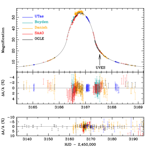
Figure 1: The upper panel shows the photometry of the microlensing event OGLE 2004–BLG–254 near its peak, on June 10, 2004, observed by four PLANET sites, Danish 1.54m, UTas 1m, Perth 0.6m, Boyden 1.5m and SAAO 1.0m and OGLE. Since the shape of the magnification curve depends on the value of each linear limb-darkening coeffecient, different for each telescope, we choose the common best value of UTas and OGLE in Tab. 1 to plot (solid line) the best-fitting point-lens, limb-darkened extended source model around the peak region. The residuals for each site are displayed by assuming their own best linear limb-darkening coefficients. The lower panel shows the residuals of the complete set of data (the two vertical lines indicate the peak region displayed above). The UVES spectrum was taken at MHJD$=3167.54159$ at mid-exposure (vertical arrow).

3.1 Extended-source formalism

With $D_{\mathrm{S}}$ denoting the source distance and $x=D_{\mathrm{L}}/D_{\mathrm{S}}$ the fractional distance of the lens, of mass $M$, the angular Einstein radius reads

$$\theta_{\mathrm{E}}=\sqrt{\frac{4GM}{c^{2}D_{\mathrm{S}}}\ \frac{1-x}{x}}.$$ (1)

which is a characteristic scale of microlensing. For a point source situated at a projected angular separation $u\ \theta_{\mathrm{E}}$ from the lens, the magnification function is given by

$$A_{\mathrm{PSPL}}(u)=\frac{u^{2}+2}{u\ \sqrt{u^{2}+4}}.$$ (2)

The magnification $A_{\mathrm{ES}}$ of an extended limb-darkened source of angular radius $\rho_{\mathrm{*}}\ \theta_{\mathrm{E}}$ is obtained by integrating $A_{\mathrm{PSPL}}$ over the source disk. With $I(r)$ being the brightness profile of the source, normalized to unit flux (Sect. 3.2),

$$\begin{array}[]{rl}A_{\mathrm{ES}}(u|\rho_{\mathrm{*}},I)&=\displaystyle\int\limits_{0}^{2\pi}\int\limits_{0}^{1}I(r)\ A_{\mathrm{PSPL}}(\eta)\ r\ \mathrm{d}\varphi\ \mathrm{d}r,\\ \mbox{where}\qquad\eta&=\displaystyle\sqrt{(\rho_{\mathrm{*}}\,r)^{2}-2\,u\,r\,\rho_{\mathrm{*}}\cos\varphi+u^{2}}.\end{array}$$ (3)

For a uniformly bright source, Witt & Mao (1994) have derived a semi-analytic expression of $A_{\mathrm{ES}}$, involving elliptic integrals. However, based on the fact that in a usual microlensing event toward the bulge of the Milky Way, extended source effects are only prominent for small lens-source angular separations ($u\ll 1$), where $A_{\mathrm{PSPL}}(u)\simeq u^{-1}$, Gould (1994) found that the extended-source magnification factorizes as:

$$A_{\mathrm{ES}}(u|\rho_{\mathrm{*}})\simeq A_{\mathrm{PSPL}}(u)\times B_{0}\left(\frac{u}{\rho_{\mathrm{*}}}\right).$$ (4)

The second factor can be expressed by the semi-analytical formula $B_{0}(z)=\frac{4}{\pi}\,z\,E\left[\arcsin\min\left(1,\frac{1}{z}\right),z\right]$ (Yoo et al. 2004) , where $E$ is the incomplete elliptic integral of the second kind. By separating the $u$ and $z=u/\rho_{\mathrm{*}}$ parameters, this formula allows easy discretization and fast computation of extended-source effects.

For non-uniform profiles (e.g. power-law limb-darkening models or tabulated profiles from stellar atmospheric models), no such simple expressions are known. Different strategies have been proposed: Witt & Mao (1994) use the uniform source magnification and its derivative in a one-dimensional integral; Heyrovský (2003) first calculates analytically the angular integral of the magnification, so that a single integral involving the (radially dependent) brightness of the source remains. Finally, Yoo et al. (2004) give expressions of $B_{1}$-and $B_{1/2}$- functions, related to the linear and square root limb-darkening laws, respectively (with the same approximations as for Eq. (4), to be numerically integrated.

When applying this formalism to OGLE 2004–BLG–254, we find that the maximal relative discrepancy between the exact magnification and its approximation related to Eq. (4) is less than $0.05\ \%$ for a linear limb-darkening law, which is well within the typical data error bars. We therefore use Eq. (4) to derive our limb-darkening coefficients.

3.2 Event model parameters

In the photometric analysis of the event, both PLANET and OGLE data are used. For each PLANET observation site, we have applied a cut on seeing which only removes very unreliable points; we restricted the complete OGLE data to the ones collected after HJD’ $=3050.0$ (which is large enough to derive the baseline magnitude). OGLE provides $128$ data points, SAAO $114$, UTas $64$, Boyden $75$ and Danish $231$, for a total of $5$ observing sites and $612$ measurements. Data reduced with our DoPhot-based pipeline underestimate photometric errors (e.g. for bright magnitudes, error estimates may reach $10^{-3}$, which is unrealistic). Comparison with the scatter of the non-variable stars suggests that the errors are underestimated by about $20\%$. Based on PLANET experience of PSF photometry used here, we rescale the errors as $\sigma_{\mathrm{resc}}^{2}=\left(1.2\ \sigma_{\mathrm{data}}\right)^{2}+(0.01)^{2}$. As the source star is a K3 giant, we first check if the fluctuation in the OGLE baseline magnitude can be due to intrinsic periodic activity (which could easily be included into the models). A power spectrum of 115 baseline data points coming from OGLE does not show evidence for modulation greater than $\sigma_{\mathrm{mod}}=0.015$. We therefore attribute the residuals in the baseline to non-periodic variability or observational noise.

As expected, a single-lens point-source model results in a high $\chi^{2}/\mathrm{d.o.f.}$ ($\sim 31$), which obviously excludes this possibility. On the other hand, a uniform extended source model provides us with a first working set of parameters that fit the data well. However, at this stage, the residuals of the fit show some symmetric trends around the peak of the light curve that indicate limb-darkening effects. We thus add linear limb darkening to the source model. This is described here by

$$I(r)=\frac{1}{\pi}\left[1-\Gamma\left(1-\frac{3}{2}\ \sqrt{1-r^{2}}\right)\right],$$ (5)

where $I(r)$ is normalized to unit total flux. The relation between $\Gamma$ and the more commonly used parameter $a$, defined by

$$I(r)\propto 1-a\left(1-\sqrt{1-r^{2}}\right),$$ (6)

is given by $a=\frac{3\,\Gamma}{2+\Gamma}$.

The parameterization involves basic microlensing parameters: $t_{\circ}$ (time of closest approach), $u_{\circ}$ (impact parameter), $t_{\mathrm{E}}$ (crossing time of the Einstein ring radius), the source size $\rho_{\mathrm{*}}$ (in units of $\theta_{\mathrm{E}}$) and two annual parallax parameters $\pi_{\mathrm{E}}$ and $\psi$ (see Sect. 5) common to all data sets, and specific parameters for each site: baseline and blending magnitudes, as well as the linear limb-darkening coefficients $\Gamma$. The values found for the latter are more fully discussed in Sec. 6. Errors on the best-fit parameters were obtained by Monte-Carlo simulations: we generate 500 sets of noisy light curves for each of the five observing sites using the obtained best-fit parameters, based on the rescaled error bars of the data; then, from the distribution of the obtained values we determine the (non-Gaussian) $68.3\ \%$ confidence intervals for each parameter. The best corresponding set of parameters fitting the data and their errors is given in Tab. 1.

Table 1: Parameters for the best-fitting point-lens limb-darkened extended source models, using linear limb-darkening law (one LLDC coefficient per data set). The set of data contains $612$ measurements coming from $4$ PLANET sites (Danish 1.54m, UTas 1m, Boyden 1.5m and SAAO 1.0m) and from OGLE. We also report the $\chi^{2}$ value.

Parameters	Value & Error
$t_{\circ}$ (days)	$3166.8194\pm 0.0002$
$u_{\circ}$	$4.60^{+0.76}_{-0.86}\leavevmode\nobreak\ \times 10^{-3}$
$t_{\mathrm{E}}$ (days)	$13.23^{+0.04}_{-0.05}$
$\rho_{\mathrm{*}}$	$4.00^{+0.00}_{-0.02}\leavevmode\nobreak\ \times 10^{-2}$
$\left.\Gamma_{I}\right|_{\mathrm{SAAO}}$ / $\left.a_{I}\right|_{\mathrm{SAAO}}$	$0.35^{+0.02}_{-0.05}$ / $0.45^{+0.03}_{-0.06}$
$\left.\Gamma_{I}\right|_{\mathrm{UTas}}$ / $\left.a_{I}\right|_{\mathrm{UTas}}$	$0.43^{+0.03}_{-0.06}$ / $0.53^{+0.03}_{-0.06}$
$\left.\Gamma_{I}\right|_{\mathrm{Boyden}}$ / $\left.a_{I}\right|_{\mathrm{Boyden}}$	$0.58^{+0.00}_{-0.03}$ / $0.68^{+0.00}_{-0.03}$
$\left.\Gamma_{I}\right|_{\mathrm{OGLE}}$ / $\left.a_{I}\right|_{\mathrm{OGLE}}$	$0.43^{+0.04}_{-0.06}$ / $0.53^{+0.04}_{-0.06}$
$\left.\Gamma_{R}\right|_{\mathrm{Danish}}$ / $\left.a_{R}\right|_{\mathrm{Danish}}$	$0.61^{+0.03}_{-0.06}$ / $0.70^{+0.03}_{-0.05}$
$\left.F_{\mathrm{B}}/F_{\mathrm{S}}\right|_{\mathrm{SAAO}}$	$0.25\pm 0.02$
$\left.F_{\mathrm{B}}/F_{\mathrm{S}}\right|_{\mathrm{Danish}}$	$0.05\pm 0.01$
$\left.F_{\mathrm{B}}/F_{\mathrm{S}}\right|_{\mathrm{UTas}}$	$0.55\pm 0.01$
$\left.F_{\mathrm{B}}/F_{\mathrm{S}}\right|_{\mathrm{Boyden}}$	$1.15\pm 0.2$
$\left.F_{\mathrm{B}}/F_{\mathrm{S}}\right|_{\mathrm{OGLE}}$	$0.00\pm 0.0$
$\chi^{2}/\mathrm{d.o.f.}$	$1326/593$

The blending fraction significantly varies from one PLANET site to another. This is a consequence of the fact that the source has two very close neighbours, one of them at a distance of $1.4^{\prime\prime}$ as stated in Sec. 2.2. Our measured blendings are consistent with the different telescopes CCD resolutions. Moreover, the low value obtained with the Danish 1.54m ($\simeq 6\%$) favors a low blend flux from the lens star.

Based on this model, we find the transit time to be $\simeq 1.05$ day and the date (where we write $t={\rm HJD}-2,450,000$) at which the lens starts to transit the source disk, $t_{\rm entry}\simeq 3166.2937$, as well as the exit time $t_{\rm exit}\simeq 3167.3451$. One can note the UVES spectra (Sec. 2.3) were taken after the end of the transit, and so only weak differential magnification over the source disk is expected (Heyrovský et al. 2000).

4 Nature of the source star

Measuring the relative proper motion and velocity at the lens distance requires a determination of the distance and radius of the source star. This can be achieved by determining the apparent magnitude at baseline, the effective temperature, the gravity, and the amount of interstellar absorption toward the source. We seek to measure these quantities by use of a combination of the obtained photometry and spectroscopy.

4.1 Source star calibrated colour-magnitude diagram

Fig. 2 shows the calibrated OGLE $(V-I)$ versus $I$ colour-magnitude diagram of the field of the source/lens. The calibrated magnitude and colour of the target are $I=16.59\pm 0.05$ and $(V-I)=2.26\pm 0.08$. A box encompasses stars belonging to the red giant clump (RC), and the two histograms give a calibrated mean position of the clump of $I^{\rm RC}=15.80\pm 0.10$ and $(V-I)^{\rm RC}=2.13\pm 0.05$. The shift in position of our target with respect to the mean red clump position is then $\Delta I=0.79\pm 0.11$ and $\Delta(V-I)=0.13\pm 0.09$.

For the absolute magnitude of the clump, we adopt the Hipparcos position as given by Stanek & Garnavich (1998), $M_{\mathrm{I}}=-0.23\pm 0.03$. The mean Hipparcos clump colour of ${(V-I)_{\circ}}^{\rm RC}=1.00\pm 0.05$ is adopted, assuming any difference with the Baade’s Window mean colour to be due to the anomalous extinction law in the Galactic Bulge, as first explained by Popowski (2000).

The Galactic Center distance modulus from Eisenhauer et al. (2005) is adopted as $\mu=14.41\pm 0.09$, but a slightly larger distance is adopted for the red clump in this field, due to its negative longitude and the bar geometry (see, e.g.: Stanek et al. 1997). The difference in distance is based on mean clump position in different regions from Sumi (2004), and amounts to $\Delta\mu=0.21\pm 0.10$, giving an adopted distance to the red clump of this field of $\mu=14.62\pm 0.13$. Therefore, the mean dereddened magnitude of the clump is ${I_{\circ}}^{\rm RC}=14.39\pm 0.14$. Comparison with its calibrated apparent magnitude and colour gives an estimate of reddening parameters as $A_{\mathrm{I}}=1.41\pm 0.17$ and $E(V-I)=1.13\pm 0.07$, the latter in very good agreement with Sumi’s measurement of $E(V-I)=1.17$ for the nearby OGLE-II field BUL-SC25. From these two independently determined values follows the total-to-selective absorption ratio $R_{\mathrm{I}}=A_{\mathrm{I}}/E(V-I)=1.25\pm 0.14$, intermediate between standard reddening law value (1.5) and Sumi’s anomalous mean value for the Galactic Bulge (0.964).

We furthermore use Girardi et al. (2002) theoretical isochrones to determine the mean metallicity of the red clump, and by adopting an age of $10$ Gyr (typical age of red clump giants in the Bulge) we find $Z^{\rm RC}\simeq 0.008$.

Finally, from the adopted position of the clump and the shift of the target, we obtain a dereddened magnitude and colour of the target as $I_{\circ}=15.18\pm 0.18$ and $(V-I)_{\circ}=1.13\pm 0.11$.

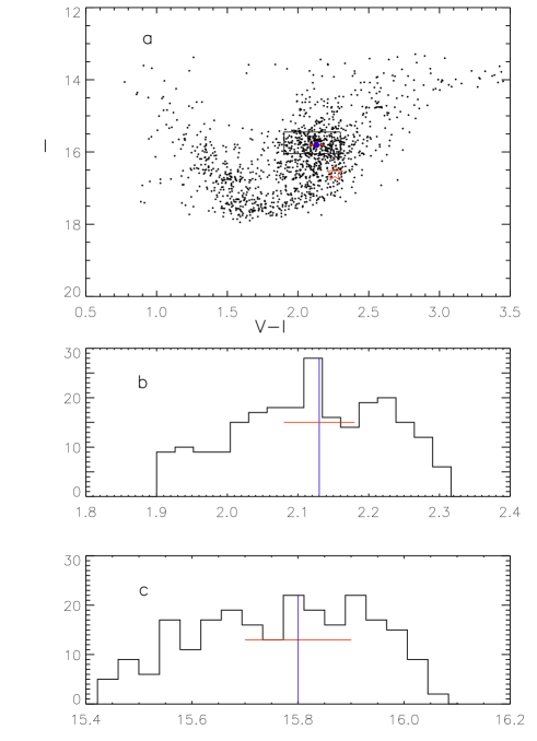
Figure 2: (a) Calibrated $(V-I),I$ colour-magnitude diagram of the field around OGLE 2004–BLG–254 as obtained with the OGLE telescope at Las Campanas. The target is plotted as a red open star. The mean position of the red giant clump is the blue dot, as determined by the color histogram (b) and magnitude histogram (c) of the stars inside the black box of panel (a). Mean positions and uncertainties are the blue and red lines respectively.

The comparison of $(V-I)_{\circ}$ with the values from the grid of model atmosphere colours by Buser & Kurucz (1992) provides an estimate of the photometric temperature of the source star. First, we note that typical changes in the theoretical value of $(V-I)_{\circ}$ for a change in metallicity by a factor of two, or a change in $\log g$ by an order of magnitude, are about $5\times 10^{-3}$ (for fundamental parameters in the range of values of interest in the present study). In comparison, a change in the value of $T_{\mathrm{eff}}$ by $100$ K gives rise to a 10 times larger change in $(V-I)_{\circ}$. The value of $(V-I)_{\circ}$ is therefore primarily a measure of the effective temperature of the star. Interpolating in the values of $(V-I)_{\circ}$ from the grid of Buser & Kurucz (1992), gives us the best fit effective temperature of the source star from the photometry alone, as $T_{\mathrm{eff}}^{\mathrm{phot}}=4500\pm 250\,\mbox{K}$. The quoted uncertainty reflects solely from the uncertainty in the estimate of $(V-I)_{\circ}$.

4.2 Source star fundamental parameters from spectroscopy

The position of the source star (and lens) is in the direction of the Sagittarius dwarf galaxy, and it could either be a member of the dwarf galaxy or of the Galactic Bulge. The line positions of the observed spectrum have a general offset of $+134$ km/s compared to laboratory data, which is also consistent with the star being in either the Sagittarius dwarf galaxy or the Galactic Bulge. The mean chemical abundance [$\@element{\mathrm{Fe}}$/$\@element{\mathrm{H}}$] ranges between $-0.8$ and $-1.2$ in Sagittarius, and around $-0.1$ in the Galactic Bulge (Fulbright et al. 2006). For the analysis of the UVES spectrum, we have therefore computed a grid of model atmospheres with $T_{\mathrm{eff}}$ between $4000$ K and $4600$ K, $\log g$ between $0.0$ and $3.0$, and scaled solar abundances with [$\@element{\mathrm{Fe}}$/$\@element{\mathrm{H}}$] between $-2.0$ and $+0.5$, and corresponding synthetic spectra.

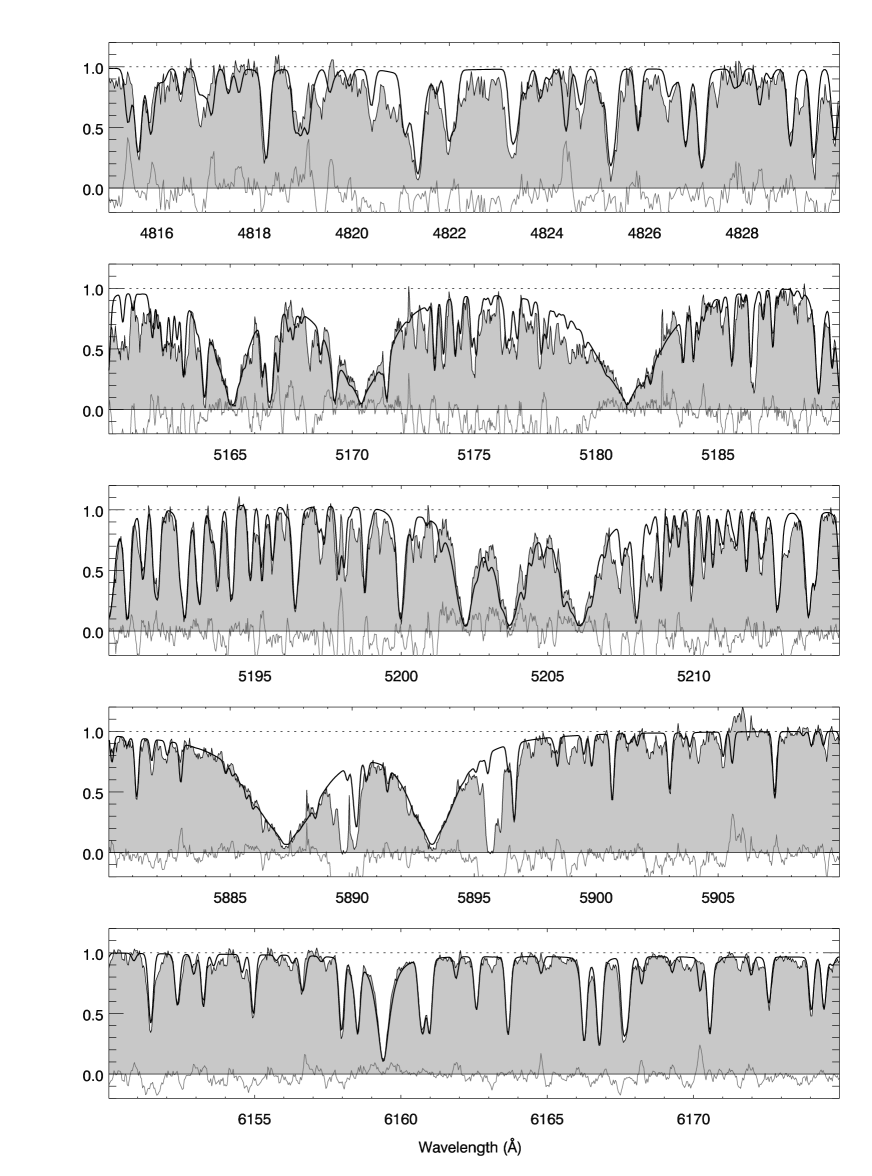
Figure 3: A comparison of the observed de-redshifted OGLE 2004–BLG–254 source star spectrum (grey) with a synthetic spectrum (thick black line) based on a model atmosphere with $T_{\mathrm{eff}}=4100$ K, $\log g=1.9$ and $Z=2.1\,Z_{\odot}$. The thin grey line around $y=0$ indicates the residual. The spectra are normalized to the local continuum. From top to bottom, the panels show the spectral region of: (2) a triplet of magnesium lines; (3) a triplet of chromium lines; (4) the NaD doublet; (1) and (5) show two other typical regions of the spectrum.

The synthetic spectra are calculated by performing 1-dimensional radiative transfer through standard Kurucz’ model atmospheres and disk-integrating the results from 7 $\mu$-angles. Spectral line data is taken from the VALD data base (Kupka et al. 1999). The observed spectrum shows approximately $10,000$ well-defined lines, and almost all of them are identifiable from comparison with line positions and strengths of the transitions listed in the vald data base. Line profiles are computed as Voigt profiles with the necessary broadening parameters taken from the data base.

Among the many atomic lines, we have selected 3 particularly well suited systems of strong $\@element{\mathrm{Mg}}$, $\@element{\mathrm{Cr}}$, and $\@element{\mathrm{Na}}$ lines, whose intensity and line shapes are fitted to constrain the possible estimates of the fundamental parameters: effective temperature $T_{\mathrm{eff}}$, gravity $\log g$, and metallicity $Z$. Other lines are used to control this estimate and to get a feeling for individual deviations from a scaled solar abundance. Fig. 3 shows the observed spectrum in those regions, together with a synthetic spectrum discussed below.

Magnesium lines – The triplet of neutral magnesium lines around $5175$ Å is well suited to obtain limits on the temperature and gravity. The line system overlaps with the position of a relatively strong $\@element{\mathrm{MgH}}$ band, and the ratio between $\@element{\mathrm{Mg}}$ and $\@element{\mathrm{MgH}}$ is sensitive to temperature as well as gravity. For strong gravity, the atomic magnesium triplet lines become very broad, but for low temperatures, the balance shifts in favour of $\@element{\mathrm{MgH}}$. Therefore, the shape and the intensity of the atomic lines can be used together with the ratio (or absence) of the intensity of $\@element{\mathrm{MgH}}$ relative to the intensity of the atomic $\@element{\mathrm{Mg}}$ lines to provide information on both temperature and gravity. The absence of $\@element{\mathrm{MgH}}$ in our observed spectrum allows us to conclude that the star is not cooler than $4000$ K. The breadth of the atomic $\@element{\mathrm{Mg}}$ lines allows us to confine the value of $\log g$ between 1.0 and 2.5. The medium-strong neutral atomic $\@element{\mathrm{Mg}}$ line at $5711$ Å is known to respond oppositely to the triplet lines to changes in gravity, i.e. to become stronger for decreasing gravity. The synthetic line is too strong for $\log g=0.0$ and solar metallicity, while it becomes too narrow for high $\log g$.

Chromium lines – As for the $\@element{\mathrm{Mg}}$ triplet region, the $\@element{\mathrm{MgH}}$ molecular system also has a relatively strong band in the region of a triplet of three strong chromium lines at $5204.51$, $5206.04$ and $5208.42$ Å, which limits $T_{\mathrm{eff}}$ to no less than $4000$ K. Models of $T_{\mathrm{eff}}=4200$ K fit the $\@element{\mathrm{Cr}}$ lines well, while models of $T_{\mathrm{eff}}=4400$ K result in wings of the lines being too weak even for high metallicity models, while $T_{\mathrm{eff}}=4000$ K would require a metallicity considerably below $Z_{\odot}$. The chromium system is less sensitive to gravity than the other two line systems, and for some $T_{\mathrm{eff}}$, even values as low as $\log g\simeq 0.0$ could be in agreement with the observed spectrum. On the other hand the lines are sensitive to the chromium abundance and $Z=0.3\ Z_{\odot}$ is too low unless $T_{\mathrm{eff}}$ is as low as $4000$ K.

Sodium lines – The intensity and form of the $\@element{\mathrm{NaD}}$ lines around $5890-5896$ Å and other neutral sodium lines are very sensitive to $T_{\mathrm{eff}}$ as well as to gravity and (sodium) abundance. Often these lines are not useful for determination of the fundamental parameters and abundances, because interstellar absorption saturates or changes their intensity. In this case, however, the main component of the interstellar absorption is redshifted by a velocity of $122$ km/s relative to the star, and the intrinsic stellar $\@element{\mathrm{NaD}}$ lines are very strong and appear to be only moderately affected by interstellar absorption. The fact that the fundamental parameters derived from the $\@element{\mathrm{NaD}}$ lines are in good agreement with the parameters derived from the other stellar lines, also indicates a small interstellar absorption at the radial velocity of the star. Model spectra from our grid with high metallicity ($Z=3\ Z_{\odot}$), high gravity ($\log g=3$) or low $T_{\mathrm{eff}}$, all give far too broad lines compared to the observed spectrum, and can therefore be excluded. Models of low gravity ($\sim 0$), high $T_{\mathrm{eff}}$ ($\sim 4400$ K) or low $Z$ ($\sim 0.3\ Z_{\odot}$) give on the other hand too narrow lines, and would require a strong interstellar component at the same radial velocity as the star.

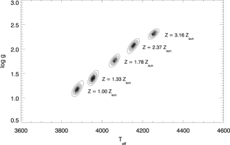
Figure 4: Using $\chi^{2}$ fitting of the spectrum to determine the most likely values of $Z$, $T_{\mathrm{eff}}$ and $\log g$ reveals a strong correlation between these parameters. Here we show the location of the minima in the $\chi^{2}$ surface for five different chosen values of [$\@element{\mathrm{Fe}}$/$\@element{\mathrm{H}}$]. Around each minimum we indicate the contours corresponding to confidence intervals of 68.3%, 95.4% and 99.7% (1, 2 and 3 $\sigma$). Treating $Z$ as a free parameter, we found the best $\chi^{2}$ solution around $T_{\mathrm{eff}}=4100$ K, $\log g=1.9$ and $Z=2.1\,Z_{\odot}$.

The intensity and form of the line systems discussed above are all different functions of $T_{\mathrm{eff}}$, $\log g$ and $Z$, and in principle three systems (like the $\@element{\mathrm{Mg}}$, $\@element{\mathrm{Cr}}$, and $\@element{\mathrm{Na}}$ systems) are sufficient to determine the three fundamental stellar parameters uniquely from the observed spectrum. In practice, of course, the observed spectrum is noisy, and the theoretical spectrum suffers from inaccuracy in the model structure, incompleteness of the line list, etc. Therefore, rather than a unique fit, there is a certain range of models which give acceptable fits to the spectrum. If $T_{\mathrm{eff}}=4300$ K is adopted, the $\@element{\mathrm{Mg}}$ lines are well reproduced by $\log g$ = 2 and $Z=Z_{\odot}$, while the $\@element{\mathrm{Cr}}$ and Na lines and most of the other lines are slightly too weak in the wings. The fit to the $\@element{\mathrm{Cr}}$ and $\@element{\mathrm{Na}}$ lines can be improved by decreasing the effective temperature to 4200 K, although this slightly decreases the goodness of the fit to the $\@element{\mathrm{Mg}}$ lines. A similar effect can be obtained by keeping the value $T_{\mathrm{eff}}=4300$ K, but increasing $\log g$ a bit, for example to $\log g=2.25$, and increasing the metallicity. At $T_{\mathrm{eff}}=4400$ K, the fit to the $\@element{\mathrm{Mg}}$ lines would still be correct, but the fit to the $\@element{\mathrm{Cr}}$ and $\@element{\mathrm{Na}}$ lines would be worse than for $T_{\mathrm{eff}}=4300$ K, and a compensation by increasing the gravity or the metallicity would require larger values than for $T_{\mathrm{eff}}=4300$ K, and therefore result in a larger decrease in the goodness of the fit to the $\@element{\mathrm{Mg}}$ system than for the $T_{\mathrm{eff}}=4300$ K model. We therefore conclude that there is no consistent solution to the fit for $T_{\mathrm{eff}}=4400$ K, and this value is therefore too large, independently of the adopted values of $\log g$ and $Z$. On the other hand, changing the temperature in the other direction, for example to $T_{\mathrm{eff}}=4000$ K, a good fit to the spectrum would require that the value of the gravity and the metallicity be decreased.

We conclude that good fits to the $\@element{\mathrm{Mg}}$, $\@element{\mathrm{Cr}}$, and $\@element{\mathrm{Na}}$ lines (and other features in the spectrum) can be obtained for models with $T_{\mathrm{eff}}$ ranging from $4000$ K to $4300$ K, $\log g$ from $1.5$ to $2.5$ and $Z$ from $1.5\,Z_{\odot}$ to $2.5\,Z_{\odot}$, which classify the star as a normal K3 III red giant. We determine the parameter values that agree best with the observed spectrum by performing a multi-dimensional $\chi^{2}$-minimization using our grid of synthetic spectra covering the range of possible valus of $T_{\mathrm{eff}}$, $\log g$ and $Z$. The optimal solution has $\chi^{2}/1504=2.997$, $T_{\mathrm{eff}}=4100$ K, $\log g=1.9$, and $Z=2.1\,Z_{\odot}$, with a covariance of $T_{\mathrm{eff}}/\log g=0.787$ and correlation coefficients of $T_{\mathrm{eff}}/\log g=0.870$, $Z/\log g=0.679$, and $Z/T_{\mathrm{eff}}=0.811$. Hence, we further conclude that there is a strong correlation between $T_{\mathrm{eff}}$, $\log g$ and $Z$ in such a way that increasing $T_{\mathrm{eff}}$ must be followed by a increased value of $\log g$ and $Z$ and vice versa. A synthetic spectrum with the optimal parameters is shown, together with the observed spectrum, in Fig. 3. In addition, we show as an illustration of the strong correlation between parameters in Fig. 4 a contour plot of the $\chi^{2}$-surface for different values of $Z$ in the plane of ($T_{\mathrm{eff}}$, $\log g$).

4.3 Source radius and distance by combining spectroscopy and photometry

In general terms, photometry has a major advantage over spectroscopy in a higher obtainable accuracy of the broadband colours than what is obtainable from integrating the spectrum (whose slope is often ill defined). With good transformation between colours and stellar effective temperatures, an accurate value of $T_{\mathrm{eff}}$ is therefore obtainable. However, a major difficulty with photometry of distant stars in the Galactic plane is a large uncertainty in the estimated reddening. We have partly got around this problem by applying the red giant clump method, which reduces the reddening problem to a question of the reddening of the target relative to the red giant clump, plus a problem of defining the clump position in an observed colour-magnitude diagram of the field around the target.

The spectroscopic method, on the other hand, has the advantage of being able to simultaneously estimate the stellar effective temperature and gravity (and metallicity). The main disadvantage, for the present purpose, is an ambiguity (i.e., correlation) between the obtained values of $T_{\mathrm{eff}}$ and $\log g$. We have illustrated this correlation in Fig. 4 for the present spectrum. By demanding that our estimated stellar effective temperature satisfy both photometry and spectroscopy, we take advantage of more information than from one of the methods alone. The value of $\log g$ can then be restricted further than was possible from spectroscopy alone, by restricting the estimate of $\log g$ to the part of Fig. 4 that overlaps with the photometric estimate of $T_{\mathrm{eff}}$.

By combining the previous photometry and spectroscopy analyses, we get a very small overlap between the two ranges of effective temperature values, namely $T_{\mathrm{eff}}$ in the interval $4250-4300$ K, although it is probably realistic to enlarge this estimated interval a bit.

4.3.1 Source distance

The combination of the fundamental source star parameters with the theoretical isochrones of Girardi et al. (2002) and our calibrated colour-magnitude diagram can provide a measure of the source star distance $D_{\mathrm{S}}$. For a given range of $T_{\mathrm{eff}}$, $\log g$ and $Z$, we get from Girardi et al. (2002) isochrones the corresponding values of the source absolute magnitude $M_{I}$; the distance then comes from $M_{I}=I_{\circ}-\mu$, where $\mu=5\,\log\,D_{\mathrm{S}}/{\rm 10\,pc}$ is the distance modulus. We also require the source to be part of the Bulge, for the probability of observing a microlensing event for a source outside of the Bulge is very low.

By assuming a temperature in the range $T_{\mathrm{eff}}=4250-4300$ K, we find no solution, whatever the age, gravity or metallicity, as illustrated in panel (a) of Fig. 5. This discrepancy between photometric and spectrocopic temperature cannot originate from a higher magnification of the limb of the source, since the transit of the lens was already finished when the UVES spetra were obtained and the corresponding effect is weak (Sec. 3.2). Fulbright et al. (2006) also reported discrepancies for Bulge K-giants, with systematic differences in photometric and spectrocopic temperatures.

We then examine the case of higher temperatures ($T_{\mathrm{eff}}>4300$ K). We first remark that the larger the distance, the smaller the temperature has to be. the optimal solution is then found for the maximum possible distance compatible with the source beeing a Bulge star, which we assume to be $D_{\mathrm{S}}=10.5$ kpc. Moreover, this compromise is better when the age of the source is maximal, which means $\simeq 16$ Gyr in Girardi et al. (2002) isochrones. A possible blend of the source star by the lens would also imply even more discrepant results, and following Sec. 3.2, we choose to neglect it. We study now the results involving different metallicities. By setting for the source the red clump metallicity, $Z\simeq 0.008$ (Sec. 4.1), we obtain a solution with $T_{\mathrm{eff}}\simeq 4575$ K and $\log g\simeq 2.36$, and a source at the distance $D_{\mathrm{S}}\simeq 10.5$ kpc. Although $T_{\mathrm{eff}}$ is still compatible with our photometric analysis of Sec. 4.1, it is above the higher bound of the allowed spectroscopic range of temperatures. The corresponding solution is shown in panel (b) of Fig. 5. If we adopt a solar metallicity, then our requirement to have $D_{\mathrm{S}}<10.5$ kpc leads to a best solution with $T_{\mathrm{eff}}\simeq 4620$ K, $\log g\simeq 2.31$ with $D_{\mathrm{S}}=10.5$ kpc, which implies similar conclusions than when assuming the red clump metallicity. This case is shown in panel (c) of Fig. 5. We do not find any satisfying solution for higher metallicity.

In conclusion, we adopt the maximum distance compatible with the source star being part of the Bulge, $D_{\mathrm{S}}\simeq 10.5$ kpc, as a best compromise between photometric and spectroscopic analysis.

4.3.2 Physical radius of the source

The value of the source distance $D_{\mathrm{S}}$ derived above combined with the angular size of the source $\theta_{\mathrm{*}}$ is now used to determine the physical radius of the source, $R_{\mathrm{*}}=\theta_{\mathrm{*}}\times D_{\mathrm{S}}$.

The surface brightness relation from Kervella et al. (2004):

$$\log(\theta_{\mathrm{*}}/\mu\mbox{as})=3.212-0.2\,I_{\circ}+0.421\,(V-I)_{\circ}$$ (7)

links the apparent angular radius of the source to the measured dereddened magnitude and colour of the source star. Adopting the values of Sec. 4.1, we find an apparent angular radius of $\theta_{\mathrm{*}}=4.5\pm 0.7\,\mu\mbox{as}$.

If we include a possible difference in reddening between the source and the red giant clump, we can write the real dereddened magnitude and colour of the source as:

$$I_{\circ} = 15.18\pm 0.18-R_{\mathrm{I}}\,\Delta E(V-I),$$ (8)

$$(V-I)_{\circ} = 1.13\pm 0.11-\Delta E(V-I),$$ (9)

where $\Delta$ is in the sense source minus red clump. From this, we get an apparent angular radius:

$$\log(\theta_{\mathrm{*}}/\mu\mbox{as})=0.652-k\,\Delta E(V-I),$$ (10)

where the coefficient of the differential extinction $k\equiv 0.421-0.2\,R_{\mathrm{I}}$ reads $0.17\pm 0.05$ for our adopted value of $R_{\mathrm{I}}$. However, a differential reddening is unlikely, since it would imply a smaller reddening for a star behind the red clump, which is somehow unsatisfactory.

Thus, assuming no differential extinction, we derive a value of $R_{\mathrm{*}}\simeq 10.2\,R_{\odot}$. We also checked that by using the simple relation $L\propto R_{\mathrm{*}}^{2}\times T^{4}$, where $T$ and $L$ are deduced from the isochrones for a source star fulfilling the conditions shown in panel (b) or (c) of Fig. 5, we find a similar result ($\pm 2\%$) for the source radius.

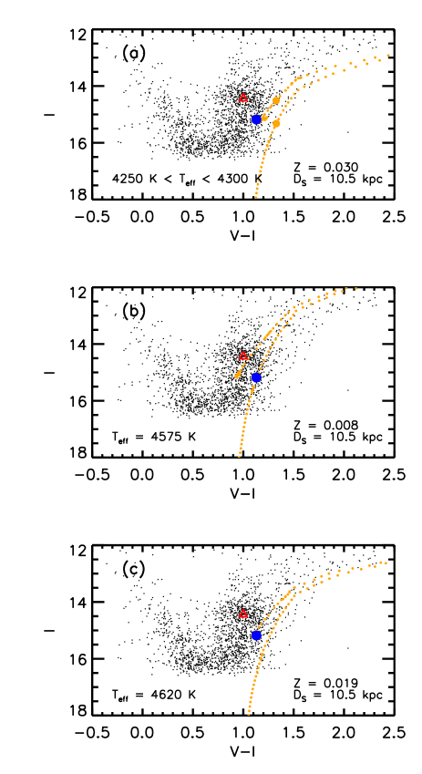
Figure 5: Same colour-magnitude diagrams as in Fig. 2. The de-reddened red clump is the red triangle, the source is the blue dot. Isochrones with metallicity $Z$ given in the right corner of each figure are plotted in light orange. Photometric temperature $T_{\mathrm{eff}}$ and source distance are also indicated. An agreement between photometric and spectroscopic observations is obtained when the source lies on the isochrone, the vertical position of which determines the source distance. In panel (a), it is seen that by setting the range of temperatures $T_{\mathrm{eff}}=4250-4300$ K from the spectroscopy analysis, no satisfying solution can be found. In fact, the two bigger dots on the isochrones matching this criterion would require a redder source and a distance which would put the source outside of the Bulge. Moreover, since the absolute magnitude of the target already agues for a source on the far end of the Bulge, a differential magnification of the source relative to the clump would require the isochrone to be at the left side of the blue dot, which would lead to even higher distances. If we allow a higher temperature, solutions can be found with our requirement that $D_{\mathrm{S}}<10.5$ kpc. Panel (b) shows the solution with the derived clump metallicity ($Z=0.008$), and panel (c) with a solar metallicity. No solution is found for higher metallicities.

5 The lens location

With the angular Einstein radius being related to the angular source radius $\theta_{\mathrm{*}}$ as $\theta_{\mathrm{E}}=\theta_{\mathrm{*}}/\rho_{\mathrm{*}}$, we find $\theta_{\mathrm{E}}\simeq 112\,\mu$as. This enables us to calculate the the relative lens-source angular proper motion: $\mu=\theta_{\mathrm{E}}/t_{\mathrm{E}}\simeq 3.1$ mas/yr. The relative velocity $v$ between lens and source at the lens distance then follows from $v=D_{\mathrm{L}}\,\mu$.

In principle, a measurement of the source size both in Einstein radius and physical units, as well as the measurement of parallax parameters completely determine the lens location (given the source distnce $D_{\mathrm{S}}$).

The source-size parameter $\rho_{\mathrm{*}}$ (in Einstein units) is well-constrained by our photometric model (Sec. 3.2), and from the value of $R_{\mathrm{*}}$ derived in Sec. 4.3.2, we obtain a constraint on the lens mass $M$ as (Dominik 1998):

$$\frac{M}{M_{\odot}}(x)=\frac{{c^{2}}}{4\,GM_{\odot}}\frac{1}{D_{\mathrm{S}}}\frac{R_{\mathrm{*}}^{2}}{\rho_{\mathrm{*}}^{2}}\frac{x}{1-x},$$ (11)

where $x=D_{\mathrm{L}}/D_{\mathrm{S}}$.

Figure 6: Probability densities for the lens mass $M$, the lens distance $D_{\mathrm{L}}$ and the relative transverse velocity $v$ at the lens distance, assuming a source distance of $D_{\mathrm{S}}=10.5\leavevmode\nobreak\ \mbox{kpc}$ and the adopted Galaxy model.

Similarly to Eq. (11), a measured parallax parameter would provide a relation between lens mass and $x$, but unfortunately the event is too short ($\sim 13$ days $\ll$ 1 year) to provide a measurement of the parallax, or even to give reasonable limits: values as different as $\pi_{\mathrm{E}}\sim 0.01$ and $10$ are hardly distinguishable from the light curve fit. For a very similar event (duration $t_{\mathrm{E}}\simeq 13$ days, source size $\rho_{\mathrm{*}}\simeq 0.06$ and very small impact parameter $u_{\circ}$), Yoo et al. (2004) only obtained a marginal parallax measurement too.

We then use estimates of the physical parameters, following Dominik (2006) and assuming his adopted Galaxy model. The event time-scale $t_{\mathrm{E}}=13.23\leavevmode\nobreak\ \mbox{days}$ and the source-size parameter $\rho_{\mathrm{*}}=0.04$ provide us with probability densities for the lens mass $M$, the lens distance $D_{\mathrm{L}}$, and the relative transverse velocity $v$ at the lens distance, which are shown in Fig. 6.

From these, we find a lens mass $M\simeq 0.11\,M_{\odot}$, a velocity $v\simeq 145\leavevmode\nobreak\ \mbox{km}\,\mbox{s}^{-1}$, and a lens distance $D_{\mathrm{L}}\simeq 9.6\leavevmode\nobreak\ \mbox{kpc}$ for an assumed source distance of $D_{\mathrm{S}}=10.5\leavevmode\nobreak\ \mbox{kpc}$. The lens is preferred to reside in the Bulge, with $58\,\%$ probability, even though with a source on the far end of the Bulge, disk lenses play a prominent role with $42\,\%$ probabilty for a disk lens scenario.

Finally, similarly to the discussion of event OGLE 2002-BLG-069 (Kubas et al. 2005), we put upper limits on the lens mass based on the measured blend ratio $F_{\mathrm{B}}/F_{\mathrm{S}}$, assuming a luminous main-sequence lens star and a source at $D_{\mathrm{S}}\simeq 10.5$ kpc. The latter limits, presented in Fig. 7, are compatible with the lens being an M dwarf in the mass regime derived in Fig. 6.

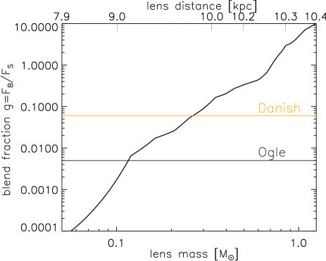
Figure 7: Assuming the fraction of blended light being solely due to the lens, upper limits on the lens mass can be derived from the measured blend ratio $F_{\mathrm{B}}/F_{\mathrm{S}}$. The implied blend ratio for range of main sequence lens stars of spectral types M0–A9 is plotted as a function of the lens distance (lower horizontal axis), or equivalently as a function of the lens mass (upper horizontal axis) given Eq. (11). The derived values are compatible with the M dwarf lens of mass $\sim 0.05-0.3\leavevmode\nobreak\ M_{\odot}$.

6 Limb-darkening measurements

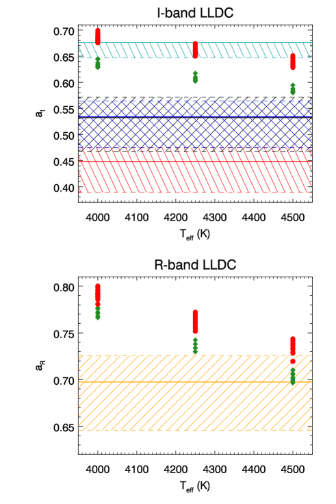
Figure 8: Linear limb-darkening coefficients (LLDC) for the I-band data sets (upper panel, from bottom to top: SAAO 1.0m, OGLE, UTas 1m and Boyden 1.5m) and the R-band data set (lower panel, Danish 1.54m). The colors follow the same convention as for Fig. 1. The best value for each $\Gamma$-coefficient is indicated by an horizontal line, where the filled area enclose the one-$\sigma$ error bar for each parameter. For the I-band, UTas 1m and OGLE give consistent values, while SAAO 1.0m and Boyden 1.5m are well below or above the latter ones (see text for a detailed discussion). Model atmosphere LLDCs: filled red dots correspond to the Claret (2000) LLDCs while the green squares correspond to the “new fit” LLDCs (see text), both for a range of temperature, $T_{\mathrm{eff}}=4000$, $4250$, $4500$ K (in abscissa), $logg=1.5$, $2.0$, $2.5$ and $[\@element{\mathrm{Fe}}/\@element{\mathrm{H}}]=0.0$, $0.1$, $0.2$, $0.3$, $0.5$, compatible with OGLE 2004–BLG–254 stellar parameters.

The photometric data of OGLE 2004–BLG–254 were dense enough to measure limb darkening of the source. Because of the duration of the event, the data coverage from a single site is not sufficient for such a measurement. Here, we benefit from our round-the-clock follow-up that permits monitoring the event over the full course of the caustic passage. We find that a square root limb-darkening law $I(r)=\frac{1}{\pi}\left[1-\Gamma\left(1-\frac{3}{2}\ \sqrt{1-r^{2}}\right)-\Lambda\left(1-\frac{5}{4}\ (1-r^{2})^{1/4}\right)\right]$ does not improve the fit, and the strong correlation between $\Gamma$ and $\Lambda$ leads to an unsatisfactory and ambiguous result.

The limb-darkening coefficients (hereafter LLDC) derived from our best fitting model for the I- and R-band are presented in Tab. 1 and Fig. 8. For each data set, the best fitting value is plotted as an horizontal line, within the a filled area that encompasses the allowed values at the one-$\sigma$ error level. The color conventions are identical to those of Fig. 1. We first note the very good agreement between the I-band OGLE and UTas 1m LLDC measurements, while SAAO 1.0m and Boyden 1.5m are not consistent with the latter values. We justify this by the fact that the peak region best constrains the LLDC, especially the shape of the top of the light curve. As a matter of fact, UTas 1m shows a good coverage of this region, as well as OGLE and Danish 1.54m, as seen in Fig. 1. However, even though SAAO 1.0m should also give good constraints, a high scatter in the peak region ruins the reliability of the measurement, and Boyden 1.5m exhibits large scater and has no baseline data points. Thus we posit the LLDC coming from UTas 1m and OGLE (for the I-band) and Danish 1.54m (R-band) to be precise enough to be compared with atmosphere model LLDC. As a result, the LLDC values we find for the two considered bands are in disagreement with the atmosphere model. The discrepancy is reduced when higher temperatures are considered, which tends to reinforce the conclusion from stellar parameters analysis in Sec. 4.

Fig. 8 then illustrates the comparison between LLDC ATLAS atmosphere models predictions with OGLE 2004–BLG–254 measurements. The filled red dots in Fig. 8 correspond to the LLDCs predicted by Claret (2000), for a range of paramater values, i.e. $T_{\mathrm{eff}}=4000$, $4250$, $4500$ K (in abscissa), $logg=1.5$, $2.0$, $2.5$ and $[\@element{\mathrm{Fe}}/\@element{\mathrm{H}}]=0.0$, $0.1$, $0.2$, $0.3$, $0.5$, compatible with the stellar parameters of OGLE 2004–BLG–254. However, we point out that Claret’s values are obtained by least-squares fits of intensity points more or less regularly spaced in incidence angle $\mu=\sqrt{1-r^{2}}$. In terms of the radial position on the stellar disk $r$, such a fit gives very high weight to points close to the limb and very low weight to points close to the center. In order to avoid this bias, we interpolate the ATLAS points by cubic splines and perform the least-squares fits on the obtained $I(r)$ intensity profiles (Heyrovský 2006). These new LLDC values are plotted as green squares in Fig. 8. As shown in the last column of Tab. 2 for the given sources, the resulting LLDCs are systematically lower than Claret’s, in this parameter range by about $0.05$. As seen from Fig. 8, such a difference in the LLDC may correspond for example to a temperature difference of several hundred K.

Previous microlensing events have yielded nine limb-darkening measurements by several follow-up teams: six for GK giants (Albrow et al. 1999b, 2000; Fields et al. 2003; Cassan et al. 2004; Jiang et al. 2004; Yoo et al. 2004), one for a subgiant (Albrow et al. 2001), and two for main sequence stars (Afonso et al. 2000; Abe et al. 2003). The $I$-band GK giant results are the most relevant for comparison, and are summarized in Tab. 2, giving the reported LLDC alongside values derived from ATLAS models (Claret 2000) for comparison.

Event	Source characteristics				Measured LLDC	ATLAS LLDC	ATLAS
	Type	$\mathrm{T_{eff}}$	$\log g$	[$\@element{\mathrm{Fe}}$/$\@element{\mathrm{H}}$]	$a_{I}$	$a_{I}$	$a_{I}$ (new fit)
MACHO 1997–BLG–28	K2 III	4250 K	$2.0$	$0.0$	$0.83\,(\pm 15\,\%)$	$0.65$	$0.60$
MACHO 1997–BLG–41	G5–8 III	5000 K	$3.2$	$-0.2$	$0.46$	$0.58$	$0.53$
EROS 2000–BLG–5	K3 III	4200 K	$2.3$	$+0.3$	$0.54$	$0.67$	$0.62$
OGLE 2002–BLG–069	G5 III	5000 K	$2.5$	$-0.3$	$0.60$	$0.57$	0.52
OGLE 2003–BLG–262	K1–2 III	4500 K	$2.0$	$0.0$	$0.70\pm 0.13$	$0.63$	$0.58$
OGLE 2003–BLG–238	K2 III	4400 K	$2.0$	$0.0$	$0.57\pm 0.06$	$0.64$	$0.59$
OGLE 2004–BLG–254	K3 III	$4000-4300$ K	$1.5$–$2.5$	$+0.2$–$+0.4$	$0.53\leavevmode\nobreak\ ^{+0.04}_{-0.06}$	0.63 (closer)	0.58 (closer)

Table 2: Limb-darkening coefficients for the $I$-band of GK Bulge giants in OGLE 2004–BLG–254 and published events. The column ATLAS LLDC is from Claret (2000), whereas the last column is a new fit to ATLAS model atmosphere intensities. The best measured LLDC for OGLE 2004–BLG–254 correspond to $T_{\mathrm{eff}}=4500$ K, $\log g=1.5-2.5$ and [$\@element{\mathrm{Fe}}$/$\@element{\mathrm{H}}$]$=0.-0.1$, based on the LLDC derived from UTas and OGLE data (see text). The ATLAS values given here are the closest to the measured ones (cf. Fig. 8).

We exclude three cases from Tab. 2 for our comparison: OGLE 2002–BLG–069 because it is of earlier spectral type; MACHO 1997–BLG–41, also of earlier type, for it suffers from correlations between the LLDC and other model parameters, and OGLE~2002–BLG–262 which has large uncertainties due to sparse temporal coverage. The four remaining objects are all K giant stars. The comparison between LLDC measurements and ATLAS atmosphere models are presented in Tab. 2. MACHO 1997–BLG–28, involved a cusp passage and seems to deviate from theory. While we do not mistrust the underlying light curve model, the accuracy of its derived limb-darkening coefficient is not sufficient to challenge the atmosphere modelling: an uncertainty of $15$–$20\leavevmode\nobreak\ \%$ seems reasonable and removes part of the apparent discrepancy. Assuming Claret (2000) limb-darkening coefficients for the stars with their known temperature, the two remaining literature events, EROS 2000–BLG–5 and OGLE~2003–BLG–238 – together with OGLE 2004–BLG–254 –, appear to disagree with theory predictions, considering the high quality and suitability of the data for a direct surface-brightness profile constraint. However, assuming our “new fit” limb-darkening coefficients, OGLE 2003–BLG–238 now agrees with the prediction, EROS 2000–BLG–5 is much closer to the predicted model, and the discrepancy for OGLE 2004–BLG–254 is reduced.

There is still an incompatibility between the measured and theoretical limb darkening of Bulge K-giant stars, as previously for EROS 2000–BLG–5 (Fields et al. 2003). However, if a limb-darkening coefficient following our fitting prescription is used, the discrepancy is significantly smaller than with the coefficients published by Claret (2000).

Finally, a comparison between the shape of synthetic atmosphere models and linear and square-root limb-darkening law curves suggests that the classical laws are too restrictive to fit well the microlensing observations, as already suggested by Heyrovský (2003). For example, all the normalized curves derived from the classical laws are constrained to pass through the point at $r=\sqrt{5}/3$, whereas curves derived from synthetic spectra of giant stars tend to intersect $\sim 5$ % closer to the center. If the latter is closer to reality, the LDC inferred from a given microlensing event might be biased by the attempt to compensate for the too steep outer behaviour of the linear limb-darkening law, and this would only be exacerbated by any sparsity in the photometric coverage at that phase. We note here that Heyrovský (2003) using simulated single-lens microlensing light curves showed that the accuracy of recovering linear limb-darkening coefficients is limited by the inadequacy of the linear limb-darkening law. Heyrovský (2003) suggests addressing this problem using a principal component analysis (PCA) approach, where orthogonal basis functions extracted from a grid of atmosphere models are used to describe the broad-band limb darkening of stars. This will be investigated in a forthcoming paper together with a set of similar single lens events with finite source effects.

7 Summary and conclusion

We have performed dense photometric monitoring of the microlensing event OGLE 2004–BLG–254, a relatively short duration and small impact parameter microlensing event generated by a point-like lens transiting a giant star. The peak magnification was about $A_{\circ}\sim 60$, effectively multiplying the diameters of our network telescopes by a factor $\sim 8$. High-resolution spectra were taken using the UVES spectrograph at La Silla while the source was magnified by a factor $A\sim 20$, just after the end of the transit of the source over the caustic. This yielded a precise measurement of the characteristics of the star, a K3 III giant, although a discrepancy is found between photometric and spectroscopic temperature. Using a calibrated colour-magnitude diagram analysis and isochrones, we find a source angular radius $\theta_{\mathrm{*}}\simeq 4.5\pm 0.7\,\mu\mbox{as}$, and a physical radius $R_{\mathrm{*}}\simeq 10.2R_{\odot}$ with the source distance $D_{\mathrm{S}}=10.5$ kpc. A Galaxy model together with the event time-scale $t_{\mathrm{E}}=13.23\leavevmode\nobreak\ \mbox{days}$ and the source-size parameter $\rho_{\mathrm{*}}=0.04$ yielded a lens mass $M\simeq 0.11\,M_{\odot}$, a lens distance $D_{\mathrm{L}}=9.6\leavevmode\nobreak\ \mbox{kpc}$, and a velocity $v\simeq 145\leavevmode\nobreak\ \mbox{km}\,\mbox{s}^{-1}$ at the lens distance. From our photometric data, we have derived measurements of the source limb-darkening coefficients for the $I$ and $R$ broadband filters, and provided arguments for a discussion about a lack of relevant physics in K-giants atmosphere models, or an inadequacy of the linear limb-darkening law to model.