Spectropolarimetry of the Classical T Tauri Star TW Hydrae

Abstract

We present high resolution ($R\approx 60,000$) circular spectropolarimetry of the classical T Tauri star TW Hydrae. We analyze $12$ photospheric absorption lines and measure the net longitudinal magnetic field for 6 consecutive nights. While no net polarization is detected the first five nights, a significant photospheric field of $B_{\rm{z}}=149\pm 33$ G is found on the sixth night. To rule out spurious instrumental polarization, we apply the same analysis technique to several non-magnetic telluric lines, detecting no significant polarization. We further demonstrate the reality of this field detection by showing that the splitting between right and left polarized components in these 12 photospheric lines shows a linear trend with Landé $g$-factor times wavelength squared, as predicted by the Zeeman effect. However, this longitudinal field detection is still much lower than that which would result if a pure dipole magnetic geometry is responsible for the mean magnetic field strength of $2.6$ kG previously reported for TW Hya. We also detect strong circular polarization in the He I $5876$ Å and the Ca II $8498$ Å emission lines, indicating a strong field in the line formation region of these features. The polarization of the Ca II line is substantially weaker than that of the He I line, which we interpret as due to a larger contribution to the Ca II line from chromospheric emission in which the polarization signals cancel. However, the presence of polarization in the Ca II line indicates that accretion shocks on Classical T Tauri stars do produce narrow emission features in the infrared triplet lines of Calcium.

1 Introduction

T Tauri stars (TTSs) are newly formed low-mass stars that have recently become visible at optical wavelengths. These young, roughly solar mass stars are still contracting along pre-main sequence evolutionary tracks in the H-R diagram. It is generally believed that classical T Tauri stars (CTTSs) are still surrounded by disks of material that are undergoing accretion onto the central star, producing excess emission in both lines and continuum at multiple wavelengths. Magnetospheric accretion models are the most popular description of the accretion process. Strong, stellar magnetic fields are believed to regulate the accretion and confine disk material to flow onto the stellar surface along the field lines (e.g., Camenzind 1990; Königl 1991; Cameron & Campbell 1993; Shu et al. 1994). These models generally assume the magnetic structure of TTSs to be dipolar and require magnetic field strengths which vary over a wide range of values, with the field on some stars as high as several kilogauss (see Johns–Krull, Valenti & Koresko 1999b). Such high field strengths should be measurable by utilizing the most magnetically sensitive diagnostics.

On the other hand, direct magnetic field measurements are difficult, since T Tauri stars are relatively faint and display various spectral peculiarities. The most successful approach for measuring fields on late–type stars in general has been to measure Zeeman broadening of spectral lines in unpolarized light (e.g., Robinson 1980; Saar 1988; Valenti, Marcy & Basri 1995; Johns–Krull & Valenti 1996; Johns–Krull et al. 1999b; Johns–Krull, Valenti, & Saar 2004). This method is more efficient at infrared wavelengths thanks to the $\lambda^{2}$ dependence of Zeeman broadening, compared to the $\lambda^{1}$ dependence of Doppler broadening. While a sensitive measure of field strength, Zeeman broadening measurements give little information on the magnetic field geometry.

Another direct method for measuring magnetic fields is to detect net circular polarization in Zeeman-sensitive lines. Generally, Zeeman $\sigma$ components are elliptically polarized and the components of opposite helicity are split to either side of the nominal line wavelength. A net longitudinal component of the magnetic field makes components of Zeeman-sensitive lines distinguishable through a right-circular polarizer (RCP) and left circular polarizer (LCP). The separation between the line observed in RCP and LCP light is

$$\Delta\lambda=2{e\over 4\pi m_{e}c^{2}}\lambda^{2}g_{\rm{eff}}B_{\rm{z}}=9.34\times 10^{-7}\lambda^{2}g_{\rm{eff}}B_{\rm{z}}\,\,\,\,\,\,\rm m\mbox{\AA}\,$$

where $g_{\rm{eff}}$ is the effective Landé $g$-factor of the transition, $B_{\rm{z}}$ is the strength of the mean longitudinal magnetic field in kilogauss, and $\lambda$ is the wavelength of the transition in Angstroms (see Mathys 1988, 1991). The weights for individual $\pi$ and $\sigma$ components in the definition of $g_{\rm eff}$ assume an optically thin medium, so eq.[1] is only approximately true in our case of moderately strong photospheric lines. Previously, Johns–Krull et al. (1999a) did not detect polarization in the photospheric lines of the CTTS BP Tau, setting a $3\sigma$ upper limit on $B_{\rm z}$  of $\pm 200$ G. Smirnov et al. (2003) report a longitudinal magnetic field of $B_{\rm{z}}\sim 150\pm 50$ G on the CTTS T Tau, which is very close to their detection limit, while their subsequent observation of T Tau (Smirnov et al. 2004) did not detect a significant field. In an effort to confirm the original Smirnov et al. (2003) detection, Daou et al. (2006) measure a mean longitudinal field of $B_{\rm z}$$\,=12\,\pm\,35$ G on T Tau. Daou et al. (2006) use upper limits on $B_{\rm z}$  on multiple nights along with the mean field strength detected on T Tau of $\bar{B}\sim 2.4\$kG (Guenther et al. 1999; Johns–Krull et al. 2001) to seriously question the assumed dipole field geometry (see also Valenti & Johns–Krull 2004).

On the other hand, Johns–Krull et al. (1999a) discovered net polarization in the He I $5876$ Å emission line on the CTTS BP Tau, indicating a net longitudinal magnetic field of $2.46\pm 0.12$ kG in the line formation region. This He I emission line is believed to be produced, at least partially, in the shock region formed where disk material accretes onto the stellar surface (Hartmann, Hewett & Calvet 1994; Edwards et al. 1994). Circular polarization in the He I line has now been observed in several CTTSs (Valenti & Johns–Krull 2004; Symington et al. 2005). These observations suggest that accretion onto CTTSs is indeed controlled by a strong stellar magnetic field.

While substantial observational evidence indicates strong fields on the surface of TTSs, the origin of the surface magnetic fields on TTSs are not clear. Interface dynamo models (e.g., Parker 1993) which are applied to solar-type main-sequence stars probably do not apply to TTSs since their internal structure is significantly different from that of the Sun. Feigelson et al. (2003) summarize several theoretical considerations for the origin of TTS magnetic fields. One possibility is that a distributed dynamo due to turbulent convection could operate in TTSs and generate small-scale magnetic fields. These fields could also be amplified by differential rotation throughout the convective zone (Durney et al. 1993; Kitchatinov & Rüdiger 1999; Küker & Stix 2001), though surface differential rotation is weak or absent on TTSs (Johns-Krull 1996). It is also possible that T Tauri stars simply maintain a “fossil” magnetic field throughout the star formation process and do not have significant field contributions from dynamo processes (Tayler 1987; Mestel 1999; Moss 2003). More observational studies are needed to put further constraints on theories of the origin and evolution of magnetic fields on pre-main sequence stars.

In order to gain further insight into the magnetic properties of young stars, we present an analysis of high resolution spectropolarimetry of the CTTS TW Hya, a K7Ve(Li) star (Herbig 1978) located at a distance of $56\pm 7$ pc (Wichmann et al. 1998). Imaging in multiple wavelengths (e.g., Krist et al. 2000; Weinberger et al. 2002; Qi et al. 2004) indicates a nearly face-on disk around TW Hya that is optically thick in the visible, near-IR, sub-millimeter and millimeter wavelengths. Herczeg et al. (2004) estimate an accretion rate of $2\times 10^{-9}$ ${\rm M}_{\odot}\ {\rm yr}^{-1}$ from its strong optical and near-UV excess emission. Previously, we have modeled magnetic broadening of four K band Ti I lines observed in unpolarized light to measure a mean magnetic field strength of $\bar{B}=2.6\pm 0.2$ kG on TW Hya (Yang, Johns–Krull & Valenti 2005). Here, we use a time series of spectropolarimetric observations to study the geometry of the stellar magnetic field. The remainder of this paper is organized as follows. In § 2 we describe our observations and data reduction procedures. In § 3 we present the measurements of the longitudinal field in the photosphere as well as in the accretion regions. H$\alpha$ line profiles are also presented in § 3. Finally, a discussion of our results is presented in § 4.

2 Observations and Data Reduction

We obtained spectra using a Zeeman analyzer (ZA) system on the 2.7 m Harlan J. Smith Telescope at McDonald Observatory on April 21-26, 1999. This system has been described by Vogt et al. (1980), with subsequent modifications described by Johns–Krull et al. (1999a). The ZA splits stellar light coming to a focus on the slit into two parallel beams that create two separate stellar images on the spectrograph slit. One beam contains approximately half the unpolarized light and any RCP light, while the other beam contains the remainder of the unpolarized light and any LCP light.

The ZA was used with the 2-d coudé cross-dispersed echelle spectrometer (Tull et al. 1995). This spectrometer provides a 2-pixel spectral resolution of $R\equiv\lambda/\delta\lambda\approx 60,000$ and enough space between the orders to interleave simultaneously stellar spectra of both circular polarization states. To reduce spurious linear polarization induced by the coudé mirror train, the ZA control computer automatically updates the retardance of a Babinet-Soleil phase compensator (PC) fixed to the front of the ZA. The phase compensation is continually changed, as telescope orientation changes throughout an observation. Each night, 2 exposures of TW Hya were obtained. Before the second exposure, an achromatic 1/2-wave plate (manufactured by Special Optics, model No. 8-9012-1/2) was inserted in front of the ZA+PC in order to switch the sense of circular polarization recorded in the two interleaved spectra. Analyzing and averaging the results of this pair of exposures reduces potential sources of systematic/instrumental error in the measurements. All spectra were reduced using an echelle-reduction package developed by Valenti (1994) and described more fully in Hinkle et al. (2000). Wavelength solutions are determined from spectra of a Thorium-Argon lamp by performing a two-dimensional fit to the positions of lines on the detector as a function of $n$ and $n\lambda$, where $n$ is the echelle order. Table 1 summarizes the observations discussed here.

3 Analysis

3.1 Photospheric $B_{\rm{z}}$

We use 12 photospheric absorption lines that have relatively large Landé $g$-factors to measure the longitudinal field, $B_{\rm z}$, on TW Hya. These lines are also relatively strong and unblended, and not significantly affected by telluric absorption. The species we use, as well as their wavelengths and Landé $g$-factors, are listed in the first three columns of Table 2.

Our analysis technique is as follows. We cross-correlate the LCP and RCP line profiles and measure the wavelength separation between the two spectra for each line. Using eq[1], we convert the measured wavelength separation for each line into a longitudinal magnetic field. We then use a Monté Carlo analysis to estimate the uncertainties in our measured wavelength separations. First we fit a Gaussian curve to the observed intensity profile, which is the sum of the LCP and RCP spectra for each night. By adding noise comparable to that in our observations to the Gaussian curve, we construct a pair of synthetic observations (one represents the LCP and the other the RCP component). Then we analyze these profiles in the same way as we handle the actual observations and obtain a line separation which is then translated into magnetic field strength using eq.[1]. For each individual spectral line on each night, we execute the Monté Carlo process above 100 times and measure the apparent shift (we have tried shifts of 0 and 0.5 pixels) between the synthetic LCP and RCP spectra. We then adopt the standard deviation of the corresponding Monté Carlo results as the uncertainties in our measurement of $B_{\rm{z}}$. The results for each photospheric line for each of the six nights are listed in the last six columns of Table 2. The weighted mean field values and their uncertainties for the six nights are listed in Table 1. The night-to-night variation is plotted at the bottom panel of Figure 3.

The mean longitudinal field value on April 26, 1999 is $149\,\pm\,33$ Gauss, well over the $3\sigma$ limit. If this field strength and uncertainty estimate are accurate, it represents the largest magnitude of $B_{\rm z}$ detected at a significant level on a low mass pre-main sequence star, and one of the highest $B_{\rm z}$ values detected for any low mass star (see Donati et al. 2006). To rule out spurious instrumental polarization, we apply the same technique to analyze six magnetically insensitive telluric absorption lines and find the observed wavelength separations between the LCP and RCP spectra of these lines. The telluric lines are narrower than the stellar photospheric lines, allowing wavelength separation to be measured more precisely, yielding smaller uncertainties in $B_{\rm z}$, and placing tighter limits on spurious instrumental polarization. In order to translate the observed wavelength separations into magnetic field strengths for comparison, we assign a $g_{\rm eff}$ for the telluric lines of 0.93, which is determined from the weighted mean value of $\lambda^{2}$$g_{\rm eff}$ for the 12 photospheric lines, where the weights are uncertainties in the photospheric field measurements. The field estimates from the telluric lines are given in Table 2 for each night. The recovered field strengths for the telluric lines are all consistent with no magnetic field (as they should be) to within the errors, which are typically $\sim 28$ G ($1\sigma$).

Another way to confirm the reality of the photospheric $B_{\rm z}$ measurement on the last night of observation is to look for a correlation between the measured wavelength shift and the $g_{\rm eff}$ of each line. This is perhaps the best way to establish the magnetic origin of the shifts, and hence rule out any potential instrumental effects unaccounted for. We can rewrite eq.[1] as follows:

$${\Delta\lambda\over 9.34\times 10^{-7}\lambda^{2}}=B_{\rm{z}}g_{\rm{eff}}\,\,\,\,\,\,$$

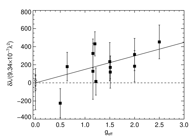
Figure 1: Plot of $\delta\lambda/(9.34\times 10^{-7}\lambda^{2})$ against Landé $g$-factors for the data from April 26, 1999. The solid line marks where $B_{\rm z}$ is equal to 149 G, the measured mean value. (Filled squares: photospheric lines; diamonds: telluric lines.)

In Figure 1, we plot the left hand side of eq.[2] against $g_{\rm eff}$. The solid line marks the expected relationship for $B_{\rm z}=149$ G. The wavelength separations of the telluric lines (hollow diamonds in Figure 1) are all found to be close to zero as they should be, since the molecular lines have negligible $g_{\rm eff}$ and form in the weakly magnetized atmosphere of the Earth. Using all the data points in Figure 1, the reduced $\chi^{2}$, $\chi^{2}_{\rm r}$, for the $B_{\rm z}=149$ G line is $0.68$, corresponding to an $83\%$ chance of being an acceptable model, while a best-fit horizontal line, indicative of an instrumental offset, yields $\chi^{2}_{\rm r}=1.91$, corresponding to less than a $2\%$ chance of being an acceptable model. The positive correlation shown in Figure 1 and the detailed statistical tests give confidence that the measured wavelength separations are indeed magnetic in origin, so that we do detect a rather strong longitudinal field on TW Hya above the $4\sigma$ limit.

Examination of Table 1 or the bottom panel of Figure 3 shows that while we find a value of $B_{\rm z}$ larger than the $3\sigma$ measurement uncertainties only once, all measurements are systematically positive and agree with each other within the uncertainties. Given that TW Hya has an inclination close to 0^∘, little rotational modulation is expected (though see §3.2). Taking the weighted mean of all 6 nights data gives a value of $B_{\rm z}$$=90\pm 17$ G.

3.2 Magnetic Fields in the Emission Line Region

Significant polarization in the He I $5876$ Å emission line has been detected on several CTTSs. Johns-Krull et al. (1999a) first discovered this polarization and found $B_{\rm z}=2.46\pm 0.12$ kG in the He I line formation region of BP Tau. Valenti & Johns-Krull (2004) found He I polarization in four CTTSs: AA Tau, BP Tau, DF Tau, and DK Tau. Symington et al. (2005) also detect He I polarization at greater than the $3\sigma$ level in three stars (BP Tau, DF Tau, and DN Tau) in their survey of seven CTTSs. While this He I line can form weakly in emission in naked TTSs (NTTSs) which are believed to lack close circumstellar disks and significant accretion, the strong He I emission of CTTSs is thought to form in the accretion shock region where disk material hits the stellar surface (e.g., Edwards et al. 1994; Hartmann, Hewett & Calvet 1994).

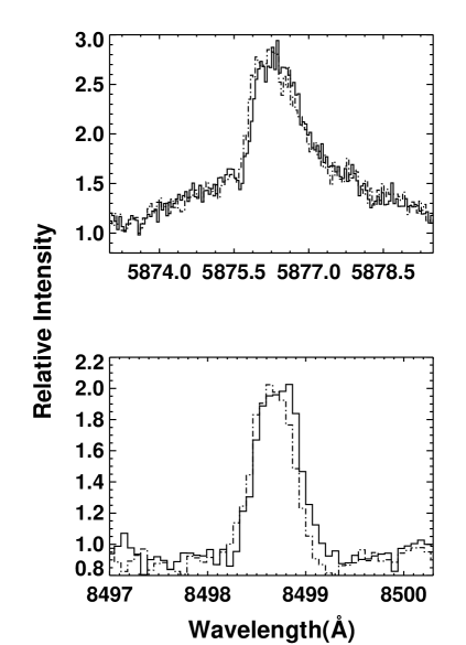
Figure 2: Observed LCP(solid line) and RCP(dash-dotted line) spectra of He I $\lambda 5876$ line and Ca II $\lambda 8498$ line on April 26, 1999.

Here we analyze our observations of TW Hya and find strong circular polarization in the He I $5876$ Å emission line as well. The same analysis technique used for the photospheric lines is applied. This He I line is a multiplet. The observed shift between the line observed in different circular polarization states described below is larger than the spacing between most of the multiplet members that make up this feature. As a result, the magnetic splitting is best described by the Paschen-Bach effect, hence $g_{\rm eff}$ = $1.0$ for the line. [Even in the weak field limit of Zeeman broadening, LS coupling gives $g_{\rm eff}$ = $1.11$ (Johns–Krull et al. 1999a), so the choice of treatment makes only a small difference on the resulting field values.] The measurements for each night are listed in Table 2 and the weighted mean of the net longitudinal field for all the nights together is $-1673\pm 50$ G. A pair of representative LCP and RCP spectra is shown in top panel of Figure 2. In addition to the 5876 Å line of He I, our spectrometer setting also contains the 6678 Å line of He I. This line is the singlet counterpart to the 5876 Å line and has $g_{\rm eff}$ = 1.0. Analysis of the 6678 Å line gives magnetic field values in the He I line formation fully consistent with the values from the 5876 Å line to within the measurement uncertainties (which are about a factor of 2 larger for the 6678 Å line since this line is weaker than the 5876 Å line).

We also detect significant polarization in the Ca II $8498$ Å emission line as shown in the bottom panel of Figure 2. Nightly measurements are given in Table 2 and we measure a weighted mean $B_{\rm z}=-276\pm 19$ G for all the nights together. We expect that the other members of the Ca II infrared triplet (IRT) show similar levels of polarization, but they fall in the gaps in our spectral coverage and were not observed. The origin of the narrow IRT emission lines seen in many CTTSs (including TW Hya) is somewhat debated and is discussed further in §4. Our detection of polarization in this line with the same polarity as the He I line suggests that the accretion shock contributes some emission to this component of the IRT. Our measured $B_{\rm z}$ for the Ca II line is 16% of our measured $B_{\rm z}$ for the He I line, which suggests at least 16% of the Ca II emission comes from accretion regions with highly ordered magnetic fields. This is a lower limit because the lower $B_{\rm z}$ for Ca II could also signify a larger contribution from regions of lower field strength (e.g., the accretion column) or mixed polarity (e.g., a radiatively heated sheath around the accretion footpoint as proposed by Batalha et al. 1996). Non-shock contribution to the He I line could lower our estimate of 16%, but in the case of TW Hya the effect is almost negligible (see more on this issue at the end of §4).

The time series of the measured field values from the He I and Ca II lines, along with that from the photosphere, are plotted in Figure 3. The night-to-night variation of the polarization in the He I line shows a hint of periodicity. We adopt a rotation period $P=2.2$ days for TW Hya from Makkaden (1998) and fit a sine wave to the measured field values. The fit has $\chi^{2}=1.2$ for 3 degrees of freedom, indicating an $76\%$ probability of being an acceptable model. However, we also fit a straight line to our data (representing a model with no variability) and find $\chi^{2}=6.30$ for 5 degrees of freedom, which has a significant $28\%$ probability of representing an acceptable model. Both fits are shown in Figure 4. The Ca II and photospheric lines do not show the same indications for periodicity; however, their relative uncertainties are much larger. Since our analysis is limited to six data points, the evidence for rotational modulation in the He I line is suggestive, but remains inconclusive.

3.3 H$\alpha$ Line Profiles

In Figure 5, we plot the H$\alpha$ profiles from all six nights. The intensity of the H$\alpha$ line varies and generally decreases with time, suggesting a possible decrease in the accretion rate on later nights. A variable blue shifted absorption component indicative of the wind from TW Hya also decreases with time over these six nights. Other than these general trends in the H$\alpha$ line over these 6 nights, nothing dramatic occurs on the last night when the photospheric $B_{\rm z}$ takes on its largest value.

We looked for circular polarization in the H$\alpha$ emission line as well. This line is very strong which aids the detection of weak line shifts between the RCP and LCP light. However, since this data was obtained with an echelle spectrometer which has a strong blaze function, continuum normalization under H$\alpha$ is not trivial. Small differences in the continuum normalization of the RCP and LCP profiles can produce spurious wavelength shifts. We attempt to quantify this by repeating the analysis of the H$\alpha$ profile using somewhat different regions to fit the continuum, as well as using polynomials of order 4, 5, and 6 in the continuum normalization process. For a given continuum fit, the strength of the H$\alpha$ line results in a $B_{\rm z}$ uncertainty of 6 G resulting from the signal-to-noise in the spectra. On the other hand, our different continuum fits on the same observed spectrum yielded field measurements different by as much as 46 G in some cases. Therefore, we conservatively adopt 46 G as the uncertainty in our H$\alpha$ $B_{\rm z}$ measurements. We did not detect a value of $B_{\rm z}$ significantly above this level on any of the nights we observed TW Hya, so we put a conservative upper limit of $B_{\rm z}$ in the H$\alpha$ line formation region of 138 G.

4 Discussion

Imaging of the circumstellar disk around TW Hya in the infrared (Krist et al. 2000; Trilling et al. 2001; Weinberger et al. 2002), millimeter (Wilner et al. 2000) and sub-millimeter (Qi et al. 2004) wavelengths all suggest that the inclination of the disk is close to $0^{\circ}$. Alencar & Batalha (2002) derived an inclination of $18^{\circ}\pm 10^{\circ}$ from emission line profile analysis. Lawson and Crause (2005) derive $i\sim 16^{\circ}$ from photometric monitoring. The night-to-night variation in our measurements of the longitudinal field in the He I line is small, only about $10\%$ of the mean value, which is also consistent with a low disk inclination angle of TW Hya. Such a geometry allows a strong test whether the magnetic field on TW Hya is primarily a dipole field with the magnetic axis aligned with the rotation axis. Yang et al. (2005) find the mean magnetic field strength in the photosphere of TW Hya to be $2.6\pm 0.2$ kG from infrared (IR) Zeeman broadening measurements. If we follow Alencar & Batalha (2002) and assume an inclination angle between $8^{\circ}$ and $28^{\circ}$, and if the magnetic dipole axis is aligned with the rotation axis, the $2.6$ kG mean field would predict a mean line of sight field in the photosphere of $B_{\rm z}$ $=0.97-1.05$ kG. This is much higher than our maximum measured value $B_{\rm z}$$=149\pm 33$ G, or our weighted mean from all nights of $B_{\rm z}$$=90\pm 17$ G. One possibility to explain the low longitudinal magnetic field values yet retain a dipole field geometry is to assume the magnetic axis is highly inclined from the rotation axis (i.e. has high obliquity, $\beta$). For example, Krist et al. (2000) use the model of Mahdavi & Kenyon (1998) and conclude that the photometric variability of TW Hya observed by Mekkaden (1998) can be explained if $i<10^{\circ}$ and the field is a dipole with $\beta>55^{\circ}$. If we take $i=10^{\circ}$ and $\beta=55^{\circ}$, the 2.6 kG mean field on TW Hya still implies a photospheric $B_{\rm z}$$=537$ G, again well above our upper limits for $B_{\rm z}$ in the photosphere. If the photospheric field is globally dipolar, then $\beta$ must be significantly larger than $55^{\circ}$. If we ask what is required of a dipole field geometry to match the 2.6 kG mean field and the 149 G longitudinal field for the visible hemisphere of the star, we find that $i+\beta=83.5^{\circ}$. However, in this case we have an additional constraint from the He I polarization.

If the photospheric magnetic field on TW Hya is dipolar, then the magnetic poles must be nearly perpendicular to the line of sight at all rotational phases (see preceding paragraph). For such a magnetic geometry, material accreted from the corotation radius ($6.3\ R_{*}$, see Johns–Krull & Valenti 2001) will land within $13^{\circ}$ of the magnetic pole. In this case, the longitudinal field of $\sim 1.7$ kG measured in the accretion region using the He I line is only the small fraction projected onto the line of sight of the true magnetic field in this region. The minimum value of the true field is $1.7\ {\rm kG}/{\rm cos(}83.5^{\circ}-13^{\circ}{\rm)}=5.1$ kG. Such a strong field in the He I line has not been observed in any of the previous studies now covering 11 CTTSs (Johns–Krull et al. 1999a; Valenti & Johns–Krull 2004; Symington et al. 2005; Daou et al. 2006). We conclude that the surface topology of the magnetic geometry on TW Hya (and likely all CTTSs) is not a $pure$ dipole. It is likely that the field topology at the stellar surface is dominated by small scale structure such as seen on the Sun. However, the dipole component of the field will fall off the least rapidly with distance from the star, so it may well be that the interaction of the stellar field with the disk is governed by a dipole geometry. Such a picture may explain the relatively smooth, sinusoid like modulation of the field traced in the He I line of the CTTSs studied by Valenti and Johns–Krull (2004).

Hartmann (1998) gives an expression for the truncation radius for an assumed dipole field geometry (his equation 8.72) derived under the assumption of spherical accretion. As discussed by Bouvier et al. (2006), this is an upper limit for a disk geometry. If we assume that the dipole component of the field on TW Hya is responsible for our detection of $B_{\rm z}$ $=149$ G on this star, we can use the equation from Hartmann (1998) to estimate a truncation radius. The estimate again depends on the inclination of the dipole component of the field with respect to our line of sight. If (as is generally the case for the Sun) we assume the dipole component is aligned with the rotation axis, assuming $i=28^{\circ}$ gives the strongest possible dipole component consistent with our $B_{\rm z}$ detection and this correponds to an equatorial field strength of 260 G. Putting this into equation (8.72) from Hartmann (1998) yields a truncation radius of 3 $R_{*}$ which is significantly less than the co-rotation radius of 6.3 $R_{*}$. Eisner et al. (2006) analyze K-band interferometry observations of TW Hya from Keck, along with previous K-band veiling and NIR photometric measurements, to conclude that the inner radius of the optically thin disk is around 0.06 AU, which corresponds to 13 $R_{*}$. While there are additional techniques that could shed light on the exact location of this inner truncation radius (e.g. linear polarimetry is a powerful technique which may help in this regard as discussed in Vink et al. 2005), the current data suggests that the system is not in equilibrium as assumed by magnetospheric accretion theories if the dipole component of the field alone is responsible for truncating the accretion disk. There are certainly higher order contributions to the total field at the surface of TW Hya which will contribute some field strength at the co-rotation radius, but just how much depends on the detailed field geometry. We suggest more work is needed to verify whether the fields on TTSs really are strong enough to truncate disks around these stars near the co-rotation radius for realistic magnetic field geometries.

As noted in §3.2, the level of polarization in the Ca II $8498$ Å line is much less than that detected in the He I line. The IRT lines of Ca II likely have contributions from different regions in CTTSs. These lines sometimes show only broad components (BC), narrow components (NC), or a mixture of the two (e.g. Alencar & Basri 2000). It is generally accepted that the BC of the IRT originates in the accretion and/or wind flows associated with CTTSs, as this component is not observed in NTTSs. However, the origin of the NC of the IRT lines is not completely clear. The Ca II $8498$ Å line of TW Hya is dominated by a NC inside a photospheric absorption line. A chromospheric origin for the NC of the IRT lines in both NTTSs and CTTSs was proposed by Hamann and Persson (1992). Batalha and Basri (1993) and Batalha et al. (1996) echo this idea, though they further suggest that accretion activity in CTTSs can enhance the chromospheric emission. They suggest that this is due to the reprocessing of radiation produced in accretion shocks as the accreting material hits the stellar atmosphere. Another possible scenario results since the accretion occurs along stellar magnetic field lines: the process may launch Alfvén waves in the magnetosphere which deposits energy in the chromosphere, heating it beyond what the star alone would do. Observationally, there is almost certainly a chromospheric contribution to this line in TW Hya and the NC of other CTTSs given the persistent appearance of NC emission in NTTSs. For example, Batalha et al. (1996) measured equivalent widths (EWs) of the Ca II $8498$ Å line for 3 K7 NTTSs, finding values which range from $0.53$ Å to $0.59$ Å. These values are weaker than our EW measurements of TW Hya ($0.69-0.98$ Å), suggesting a contribution to the line in TW Hya from more than just pure chromospheric emission. This mixture of sources can explain the relatively weak polarization observed in the Ca II line relative to the He I line. We generally expect the magnetic field in the stellar chromosphere to show the same behavior as that traced by the photospheric absorption lines. In particular, the weak photospheric polarization suggests there should be comparably weak polarization in the IRT lines, and we further expect the implied field to be of the same polarity. The field detected in the Ca II line is of opposite polarity to that observed in the photosphere, implying that the polarization in the enhanced portion of the IRT emission is more polarized than implied by the reported value of $B_{\rm z}$ in this line. The polarity of the average field in the Ca II region is the same as that in the He I region on all nights, suggesting that their emission is related. Whether this implies actual formation of (some of) the IRT NC emission in the accretion shock or formation in nearby field regions of the same polarity is not clear.

This dilution of the Ca II polarization by chromospheric emission is not expected to be an issue for the He I line. The He I $5876$ Å line of TW Hya is dominated by NC emission as well; however, the contribution to this from a pure stellar chromosphere is likely quite small. For example, Batalha et al. (1996) find the EW of the He I $\lambda 5876$ for the same 3 K7 NTTSs to range between $0.00-0.09$ Å, while for TW Hya we find values from $2.5-4.3$ Å. Besides chromospheric activities, both magnetospheric infall and a hot wind could potentially give rise to the He I emission. They are believed to be responsible for the blue-shifted or red-shifted broad components of the $5876$ Å line profiles in spectra of a number of T Tauri stars (e.g., see Baristain et al. 2001). In the case of TW Hya, an obvious BC is not seen. Thus, the He I line in TW Hya, and indeed in most CTTSs, is likely dominated by emission from the accretion shock. In the extreme case of Batalha et al. (1996), the collective non-shock contributions only account for 4% (0.09 Å/ 2.5 Å) of the He I emission, which makes our estimate that 16% of Ca II emission is from accretion regions only adjusted down by 0.6% at most.

We did not detect any polarization in the H$\alpha$ line forming region. H$\alpha$ emission likely results from several zones in the TW Hya system including the accretion shock, magnetospheric accretion flow, and the stellar and/or disk wind flowing away from the star. Thus, the line forms over a large volume where the mean magnetic field is likely relatively weak and the direction of the field is not constant. Indeed, there are regions in the magnetosphere (if viewed nearly pole-on) where the field directions are reversed. This mixture of polarities will reduce the separation of LCP and RCP line profiles. Depending on where the majority of the line forms, we expect the local field strength to be quite weak. For example, assuming a face-on disk for TW Hya and a dipolar-like magnetospheric accretion flow with the magnetic axis close to the stellar rotation axis, the dipole component of the field at the corotation radius will be equal to the stellar value of that field multiplied by $(R_{*}/R_{co})^{3}$. Taking our estimate above of 260 G for the equatorial value of the dipole component of the field at the stellar surface and $R_{co}=6.3R_{*}$ yields a field of about 1 G at a corotation radius where the magnetospheric flow may originate. This example simply illustrates that the field strength throughout a large portion of the H$\alpha$ line forming region may be quite weak, so our lack of a detection in this line may well be expected.

Table 1: Observations and Results

UT Date	UT Time	$N_{\rm{exp}}$	Total Exposure	$B_{\rm{z}}$(G)	$\sigma$
			Time(s)
1999 Apr 21	03:54	2	4300	66	40
1999 Apr 22	04:12	2	4700	54	56
1999 Apr 23	03:44	2	4700	84	32
1999 Apr 24	03:38	2	4700	82	61
1999 Apr 25	04:48	2	4700	47	48
1999 Apr 26	03:37	2	4700	149	33

Table 2: Photospheric Field Measurements.

Species	$\lambda(\rm{\mbox{\AA}})$	$g_{\rm eff}$	Apr 21	Apr 22	Apr 23	Apr 24	Apr 25	Apr 26
Ca I	6166.4	0.50	186 $\pm$ 393	-78$\pm$ 532	258$\pm$ 343	-450$\pm$ 586	76$\pm$ 316	-448$\pm$ 321
Fe I	6180.2	0.64	150 $\pm$ 350	-269$\pm$ 418	-79$\pm$ 307	-338$\pm$ 516	-20$\pm$ 349	280$\pm$ 247
Fe I	6200.3	1.51	173 $\pm$ 150	-79$\pm$ 158	52$\pm$ 102	74$\pm$ 226	238$\pm$ 143	113$\pm$ 84
V I	6213.4	2.00	-6 $\pm$ 111	30$\pm$ 159	108$\pm$ 113	145$\pm$ 224	-277$\pm$ 156	92$\pm$ 86
Fe I	6322.6	1.51	47 $\pm$ 133	14$\pm$ 328	31$\pm$ 117	-110$\pm$ 227	283$\pm$ 235	79$\pm$ 117
Fe I	6330.8	1.22	12 $\pm$ 199	233$\pm$ 258	75$\pm$ 148	74$\pm$ 281	-41$\pm$ 194	13$\pm$ 123
Fe I	6335.3	1.16	222 $\pm$ 161	244$\pm$ 245	190$\pm$ 118	540$\pm$ 273	162$\pm$ 196	280$\pm$ 138
Fe I	6336.8	2.00	76 $\pm$ 144	107$\pm$ 237	122$\pm$ 92	245$\pm$ 199	114$\pm$ 140	157$\pm$ 89
Ti I	6359.8	1.20	34 $\pm$ 145	197$\pm$ 231	110$\pm$ 112	71$\pm$ 217	317$\pm$ 148	359$\pm$ 111
Al I	6696.0	1.16	50 $\pm$ 258	101$\pm$ 337	-39$\pm$ 304	123$\pm$ 462	-11$\pm$ 372	111$\pm$ 267
Fe I	8468.4	2.50	43 $\pm$ 66	22$\pm$ 101	47$\pm$ 57	50$\pm$ 107	-53$\pm$ 92	181$\pm$ 74
Fe I	8757.1	1.50	142 $\pm$ 168	106$\pm$ 149	131$\pm$ 103	35$\pm$ 170	-112$\pm$ 181	156$\pm$ 140
Telluric	8139.5	0.90	-33 $\pm$ 88	24$\pm$ 83	55$\pm$ 95	-153$\pm$ 89	-62$\pm$ 65	-75$\pm$ 243
Telluric	8140.5	0.90	17 $\pm$ 48	124$\pm$ 51	14$\pm$ 55	78$\pm$ 62	35$\pm$ 76	-21$\pm$ 72
Telluric	8141.5	0.90	-33 $\pm$ 45	-30$\pm$ 64	-31$\pm$ 44	21$\pm$ 69	-78$\pm$ 81	25$\pm$ 57
Telluric	8146.1	0.90	-10 $\pm$ 69	-4$\pm$ 71	44$\pm$ 68	-38$\pm$ 58	-21$\pm$ 79	33$\pm$ 61
Telluric	8147.0	0.90	64 $\pm$ 68	58$\pm$ 82	34$\pm$ 66	-8$\pm$ 68	-27$\pm$ 83	27$\pm$ 69
Telluric	8158.0	0.90	-3 $\pm$ 37	3$\pm$ 47	-10$\pm$ 47	-82$\pm$ 66	-37$\pm$ 73	-17$\pm$ 51
He II	5876.	1.00	-1806$\pm$ 114	-1506$\pm$ 112	-1790$\pm$ 149	-1583$\pm$ 159	-1471$\pm$ 143	-1776$\pm$ 96
Ca II	8498.	1.07	-212$\pm$ 57	-289$\pm$ 59	-323$\pm$ 36	-392$\pm$ 62	-402$\pm$ 64	-180$\pm$ 34

Figure 3: Time series of $B_{\rm{z}}$ values measured from different spectral lines.(Top Panel: field values measured from He I $\lambda 5876$ line; Middle Panel: measured from Ca II $\lambda 8498$ line; Bottom Panel: measured from 12 photospheric lines.)

Figure 4: Time series of the longitudinal magnetic field measured by He I $\lambda 5876$ line. The solid curve is a sine wave fit with a period of 2.2 days. The dash line is a best fit model with no periodicity.

Figure 5: $\rm{H\alpha}$ line profiles from six consecutive nights.

References

- (1)
- (2) Alencar, S. H. P. & Basri, G. 2000, AJ, 119, 1881
- (3) Alencar, S. H. P. & Batalha, C. 2002, ApJ, 571, 378
- (4)
- (5) Beristain, G., Edwards, S. & Kwan, J. 2001, ApJ, 551, 1037
- (6)
- (7) Batalha, C. C. & Basri, G. 1993, ApJ, 412, 363
- (8)
- (9) Batalha, C. C., Stout-Batalha, N. M., Basri, G., & Terra, M. A. O. 1996, ApJS, 103, 211
- (10)
- (11) Camenzind, M. 1990, Rev. Modern Astron., (Berlin: Springer-Verlag), 3, 234
- (12)
- (13) Cameron, A. C. & Campbell, C. G. 1993, A&A, 274, 309
- (14)
- (15) Daou, A. G., Johns–Krull,C. M., & Valenti, J. A. 2006, AJ, 131, 520
- (16)
- (17) Donati, J.-F., Forveille, T., Cameron, A. C., Barnes, J. R., Delfosse, X., Jardine, M. M., & Valenti, J. A. 2006, Science, 311, 633
- (18)
- (19) Durney, B. R., De Young, D. S., & Roxburgh, I. W. 1993, Sol. Phys., 145, 207
- (20)
- (21) Edwards, S., Hartigan, P., Ghandour, L., & Andrulis, C. 1994, AJ, 108, 1056
- (22)
- (23) Feigelson, E. D., Gaffney, J. A. III, Garmire, G., Hillenbrand, L. A., & Townsley, L. 2003, ApJ, 584, 911
- (24)
- (25) Guenther, E. W., Lehmann, H., Emerson, J . P., & Staude 1999, A&A, 341, 768
- (26)
- (27) Hamann, F. & Persson, S. E. 1992, ApJS, 82, 247
- (28)
- (29) Hartmann, L., Hewett, R., & Calvet, N. 1994, ApJ, 426, 669
- (30)
- (31) Hartmann, L. 1998, Accretion Processes in Star Formation, Cambridge Astrophysics, ISBN: 0521785200
- (32)
- (33) Herbig, G. H. 1978, in Problems of Physics and Evolution of the Universe, ed. L. V. Mirzoyan, Publ. Armenian Academy of Sci., Yerevan, p.171
- (34)
- (35) Herczeg, G. J., Wood, B. E., & Linsky, J. L., Johns–Krull, C. M. & Valenti, J. A. 2004 AAS, Meeting 205, #156.04
- (36)
- (37) Hinkle, K., Wallace, L., Valenti, J., & Harmer, D. 2000, Visible and Near Infrared Atlas of the Arcturus Spectrum 3727-9300 Å ed. K. Hinkle, L. Wallace, J. Valenti, & D. Harmer. (San Francisco: ASP) ISBN: 1-58381-037-4
- (38)
- (39) Johns–Krull, C. M. & Valenti, J. A. 1996, ApJ, 459, L95
- (40)
- (41) Johns–Krull, C. M., Valenti, J. A., Hatzes, A. P., & Kanaan, A. 1999a, ApJ, 510, L41
- (42)
- (43) Johns–Krull, C. M., Valenti, J. A., & Koresko, C. 1999b, ApJ, 516, 900
- (44)
- (45) Johns–Krull, C. M. & Valenti, J. A. 2001, ApJ, 561, 1060
- (46)
- (47) Johns–Krull, C. M., Valenti, J. A., Piskunov, N. E., Saar, S. H., & Hatzes, A. P. 2001, ASP Conference Series, Vol. 248, 527
- (48)
- (49) Johns–Krull, C. M., Valenti, & J. A., Saar, S. H. 2004, ApJ, 617, 1204
- (50)
- (51) Kitchatinov, L. L., & Rüdiger, G. 1999, A&A, 344, 911
- (52)
- (53) Krist, J. E., Stapelfeldt, K. R., Ménard, F., Padgett, D. L., & Burrows, C. J. 2000, ApJ, 538, 793
- (54)
- (55) Königl, A. 1991, ApJ, 370, L39
- (56)
- (57) Küker, M., & Stix, M. 2001, A&A, 366, 668
- (58)
- (59) Lawson, W. A. & Crause, L. A. 2005, MNRAS, 357, 1399
- (60)
- (61) Mahdavi, A. & Kenyon, S. J. 1998, ApJ, 497, 342
- (62)
- (63) Mathys, G. 1988, A&A, 189, 179
- (64)
- (65) Mathys, G. 1991, A&AS, 89, 121
- (66)
- (67) Mekkaden, M. V. 1998, A&A,340, 135
- (68)
- (69) Mestel, L. 1999, Stellar Magnetism (Oxford: Clarendon)
- (70)
- (71) Moss, D. 2003, A&A, 403, 693
- (72)
- (73) Muzerolle, J., Calvet, N., Briceño, C., Hartmann, L., & Hullenbrand, L. 2000, ApJ, 535, L47
- (74)
- (75) Parker, E. N. 1993, ApJ, 408, 707
- (76)
- (77) Ostriker, E. C. & Shu, F. H. 1995, ApJ, 447, 813
- (78)
- (79) Qi, C., Ho, P. T. P., Wilner, D. J., Takakuwa, S., Hirano, N., Ohashi, N., Bourke, T. L., Zhang, Q., Blake, G. A., Hogerheijde, M., Saito, M., Choi, M., Yang, J. 2004, ApJ,616,11
- (80)
- (81) Robinson, R. D. 1980, ApJ, 239, 961
- (82)
- (83) Saar, S. H. 1988, ApJ, 324, 441
- (84)
- (85) Shu, F. H., Najita, J., Ostriker, E., Wilkin, F., Ruden, S., & Lizano, S. 1994, ApJ, 429, 781
- (86)
- (87) Smirnov, D. A., Fabrika, S. N., Lamzin, S. A., & Valyavin, G. G. 2003, A&A, 401, 1057
- (88)
- (89) Smirnov, D. A., Lamzin, S. A., Fabrika, S. N., & Chuntonov, G. A. 2004, Astron. Lett., 30, 456
- (90)
- (91) Symington, N. H., Harries, T. J., Kurosawa, R., & Naylor, T. 2005, MNRAS, 358, 977
- (92)
- (93) Tayler, R. J. 1987, MNRAS, 227, 553
- (94)
- (95) Trilling, D. E., Koerner, D. W., Barnes, J. W., Ftaclas, C., Brown, R. H. 2001, ApJ552, L151
- (96)
- (97) Tull, R. G., MacQueen, P. J., Sneden, C., & Lambert, D. L. 1995, PASP, 107, 251
- (98)
- (99) Valenti, J. A. 1994, Ph.D. thesis, Univ. California, Berkeley
- (100)
- (101) Valenti, J. A., Marcy, G. W., & Basri, G. 1995, ApJ, 439, 939
- (102)
- (103) Valenti, J. A., & Johns-Krull, C. M. 2004, Ap&SS, 292, 619
- (104)
- (105) Vink, J. S., Harries, T. J., & Drew, J. E. 2005 A&A, 430, 213
- (106)
- (107) Vogt, S. S., Tull, R. G., & Kelton, P. W. 1980, ApJ, 236, 308
- (108)
- (109) Weinberger, A. J., Becklin, E. E., Schneider, G., Chiang, E. I., Lowrance, P. J., Silverstone, M., Zuckerman, B., Hines, D. C., & Smith, B. A. 2002, ApJ, 566,409
- (110)
- (111) Wichmann, R. Bastian, U. Krautter, J. Jankovics, I., & Rucinski, S. M. 1998, MNRAS, 301L, 39
- (112)
- (113) Wilner, D. J., Ho, P. T. P., Kastner,J. H., & Rodríguez,L. F. 2000, ApJ, 534,101
- (114)
- (115) Yang, H., Johns–Krull,C. M., & Valenti, J. A. 2005, ApJ, 635, 466
- (116)