Accretion in $\rho$ Ophiuchi brown dwarfs: infrared hydrogen line ratios

Abstract

Context. Mass accretion rate determinations are fundamental for an understanding of the evolution of pre-main sequence star circumstellar disks.

Aims. Magnetospheric accretion models are used to derive values of the mass accretion rates in objects of very different properties, from brown dwarfs to intermediate-mass stars; we test the validity of these models in the brown dwarf regime, where the stellar mass and luminosity, as well as the mass accretion rate, are much lower than in T Tauri stars.

Methods. We have measured simultaneously two infrared hydrogen lines, Pa_β and Br_γ, in a sample of 16 objects in the star-forming region $\rho$-Oph. The sample includes 7 very low mass objects and brown dwarfs and 9 T Tauri stars.

Results. Brown dwarfs where both lines are detected have a ratio Pa_β/Br_γof $\sim 2$. Larger values, $\mathbin{\lower 3.0pt\hbox{$\hbox to0.0pt{\raise 5.0pt\hbox{$\char 62\relax$}\hss}\mathchar 29208\relax$}}3.5$, are only found among the T Tauri stars. The low line ratios in brown dwarfs indicate that the lines cannot originate in the column of gas accreting from the disk onto the star along the magnetic field lines, and we suggest that they form instead in the shocked photosphere, heated to temperatures of $\sim 3500$ K. If so, in analogy to veiling estimates in T Tauri stars, the hydrogen infrared line fluxes may provide a reliable measure of the accretion rate in brown dwarfs.

1 Introduction

In pre-main sequence stars, circumstellar disks feed matter onto their central stars over a period of a few million years. This accretion process does not significantly alter the properties of the star during most of this time; however, it can have a significant influence on the lifetime and evolution of the disks and of the planetary systems that may form. The physical conditions of the accretion process, in particular the mass accretion rate, can be investigated by studying the line and continuum emission produced by the accreting material. The model which has been more successful in explaining the accretion phenomena in T Tauri stars (TTS) is magnetospheric accretion, where the disk is truncated by the effect of a stellar magnetic field near or within the corotation radius. The disk material, which is slowly drifting radially toward the star, reaches the truncation radius and is then lifted above the disk midplane and accretes onto the star along magnetic field lines, impacting on the star at approximately the escape velocity. A shock forms on the stellar surface, creating a hot spot which emits the excess UV continuum and lines observed in TTS. Optical and IR line emission is expected to come from the accreting columns of gas, where the temperature has to be of the order of 10000 K. Magnetospheric accretion models have been developed in detail under the assumption of dipole magnetic field by, e.g., Hartmann et al. (Hea94 (1994)), Calvet and Gullbring (CG98 (1998)), Muzerolle et al. (Mea98a (1998), Mea01 (2001)), Lamzin (Lam95 (1995), Lam98 (1998)), to predict the expected amount of veiling and line profiles and intensities. They have been used to derive accretion rates for TTS, brown dwarfs (BDs), some intermediate-mass TTS and Herbig Ae stars (Gullbring et al. Gea98 (1998), Muzerolle et al. Mea01 (2001), Mea03 (2003), Mea04 (2004), Mea05 (2005), Natta et al. Nea04 (2004), Nea06 (2006), Calvet et al. Cea04 (2004), Garcia Lopez et al. Gea06 (2006)).

Testing magnetospheric accretion models is therefore very important and extensive checks have been carried out in several of the above papers. They have been mostly focussed on TTS, where it is possible to observe the accretion-driven emission over a large range of wavelengths, both in lines and continuum. Although it is likely that the topology of the stellar magnetic field is much more complex than the dipole field for which most models have been developed, the models seem able to account satisfactorily for TTS activity (see Bouvier et al. (Bou_PPV (2006) and references therein).

The situation is different for BDs, where at present the accreting matter is usually detected through optical and near-IR line emission. In fact, the vast majority of the existing estimates of $\dot{M}_{acc}$ in BDs are derived by fitting the observed H_α profiles with emission in magnetospheric accreting columns (Muzerolle et al. Mea03 (2003), Mea05 (2005), Natta et al. Nea04 (2004)) or by means of secondary indicators, such as the luminosity of the hydrogen near-IR lines or of the Ca IR triplet, which have been calibrated using the H_α-measured accretion rates (Natta et al. Nea04 (2004), Mohanty et al. Subu05 (2005)).

This paper reports the result of a project aimed at testing the capability of current magnetospheric models to describe quantitatively the accretion in very low mass objects and BDs by comparing the observed ratios of two IR hydrogen recombination lines, namely Pa_β and Br_γ, to the model predictions. These lines are seen in emission in most accreting TTS and BDs; their ratio can be measured relatively easily, and is not very sensitive to extinction. Muzerolle et al. (Mea01 (2001)) models predict that for the relativly large accretion rates of TTS ($\mathbin{\lower 3.0pt\hbox{$\hbox to0.0pt{\raise 5.0pt\hbox{$\char 62\relax$}\hss}\mathchar 29208\relax$}}10^{-8}$ M_⊙/yr), both lines are optically thick and have a ratio Pa_β/Br_γ$\sim 4$, typical of thermalized emission in a gas at about $10^{4}$ K. As $\dot{M}_{acc}$ decreases below $\sim 10^{-8}$ M_⊙/yr, first Br_γ and then Pa_β become optically thin, and their ratio increases to much larger values. The sample of TTS studied by Muzerolle et al. (Mea01 (2001)) does not have objects with very low $\dot{M}_{acc}$, and this particular prediction could not be tested. However, in our study of the accretion properties in $\rho$-Oph BDs (Natta et al. Nea04 (2004)) we found that two objects, with $\dot{M}_{acc}$$\mathbin{\lower 3.0pt\hbox{$\hbox to0.0pt{\raise 5.0pt\hbox{$\char 60\relax$}\hss}\mathchar 29208\relax$}}10^{-9}$ M_⊙/yr, have R$\sim 2$, inconsistent with magnetospheric accretion models.

Unfortunately, the two lines had not been observed simultaneously, and a chance low ratio due to time variability could not be ruled out. We present here the results of simultaneous observations of Pa_β and Br_γ in a sample of 16 objects in $\rho$-Oph, 7 of which are very low mass objects and BDs and the other 9 higher mass stars, added for comparison with the Taurus TTS. The observations and results are presented in Sec.2 and 3, respectively. The reliability of the derived line ratios is discussed in Sec.4. Comparison with the magnetospheric accretion models follow in Sec.5. Sec.6 contains summary and conclusions.

2 Observations and data reduction

2.1 Sample

Table 1: Observational and physical parameters of the $\rho$-Oph objects. Column 1: name of object; 2: spectral type; 3: J magnitude; 4: K magnitude; 5: J-band extinction; 6: luminosity; 7: mass; 8: effective temperature; 9: Pa_β equivalent width; 10: Br_γ equivalent width; 11: Pa_β/Br_γ  flux ratio; 12: mass accretion rate.

Obj.	Spectral	J	K	$A_{j}$	$L_{*}$	$M_{*}$	$T_{eff}$	Ew(Pa$\beta$)	Ew(Br$\gamma$)	R	$\dot{M}$
	Type	(mag)	(mag)	(mag)	($L_{\odot}$)	($M_{\odot}$)	(K)	(Å)	(Å)		($M_{\odot}/yr$)
ISO-Oph 002a	M0	12.838	9.545	3.1	0.55	0.4	3850	1.9$\pm 0.2$	2.1$\pm 0.3$	1.6$\pm 0.3$	-8.73
ISO-Oph 023	M7	14.844	12.143	2.4	0.04	0.04	2650	1.2$\pm 0.2$	1.6$\pm 0.2$	1.7$\pm 0.4$	-9.69
ISO-Oph 030	M6	12.57	10.92	0.9	0.07	0.06	2700	$<0.9$	$<6.0$	–	$<$-9.54
ISO-Oph 033	M8.5	16.45	13.93	2.2	0.01	0.015	2400	$<0.7$	$<2.7$	–	$<$-10.83
ISO-Oph 037	K5	15.052	10.224	3.9	0.16	0.7	4350	4.4$\pm 0.5$	0.8$\pm 0.3$	3.8$\pm 1.5$	-9.61
ISO-Oph 083	K9	12.257	9.251	3.0	0.81	0.4	3900	2.1$\pm 0.2$	$<0.9$	$>5.2$	-8.34
ISO-Oph 102	M6	12.433	10.766	0.9	0.08	0.06	2700	1.4$\pm 0.3$	1.8$\pm 0.3$	2.0$\pm 0.5$	-9.17
ISO-Oph 105	K9	12.547	8.915	4.0	1.5	0.35	3900	1.3$\pm 0.2$	$<3.0$	$>1.0$	-8.03
ISO-Oph 115	M0	15.616	11.486	3.7	0.07	0.6	3850	1.1$\pm 0.4$	$<4.8$	$>0.3$	-10.81
ISO-Oph 117	K8	13.325	9.978	3.1	0.35	0.6	3950	6.5$\pm 0.3$	3.3$\pm 0.1$	3.0$\pm 0.2$	-8.63
ISO-Oph 155	K3	11.322	7.806	3.2	3.1	1.0	4730	1.3$\pm 0.1$	$<1.8$	$>0.9$	-8.28
ISO-Oph 160	M6	14.148	11.947	1.9	0.04	0.05	2700	1.2$\pm 0.2$	2.3$\pm 0.4$	1.5$\pm 0.3$	-9.65
ISO-Oph 163	K5	11.378	8.271	2.7	1.6	0.6	4350	3.3$\pm 0.2$	1.1$\pm 0.4$	4.6$\pm 1.7$	-7.89
ISO-Oph 164	M6	13.27	11.08	1.9	0.09	0.06	2700	$<0.3$	$<2.8$	–	$<$-9.39
ISO-Oph 166	K5	10.754	8.464	2.2	1.9	0.6	4350	1.7$\pm 0.2$	$<1.2$	$>3.9$	-8.19
ISO-Oph 193	M6	13.611	11.086	2.3	0.1	0.06	2650	1.7$\pm 0.2$	1.9$\pm 0.4$	2.2$\pm 0.5$	-8.88

We have selected 16 objects in $\rho$-Oph which have been previously studied by Natta et al. (Nea02 (2002), Nea04 (2004), Nea06 (2006)); 15 of them are known to have Pa_β in emission, while in one case (ISO-Oph 033) Pa_β was not detected, and we added it to our sample because it is the lowest mass object in $\rho$-Oph with a measured J-band spectrum.

The adopted spectral type, effective temperature, luminosity and mass of the sample are given in Table  1. The spectral classification of objects in $\rho$-Oph is often very uncertain, as discussed, e.g., by Luhman and Rieke (LR99 (1999)), Wilking et al. (Wea05 (2005)), Doppmann et al. (Dea05 (2005)), Natta et al. (Nea06 (2006)). For 7 very low mass objects and BDs (ISO-Oph 023, ISO-Oph 030, ISO-Oph 033, ISO-Oph 102, ISO-Oph 160, ISO-Oph 164 and ISO-Oph 193) we adopt the stellar parameters derived by Natta et al. (Nea02 (2002)) by comparing low resolution simultaneous J, H and K spectra to template field stars and to model atmospheres. The uncertainties are of order $\pm 150$ K in T_eff, $\pm 0.2$ dex in L_⋆, $\pm 1$ mag on A_V.

For the other stars, we estimate the spectral type from the J-band medium resolution spectra obtained in this paper, as described in the Appendix. The corresponding T_eff is from Kenyon & Hartmann (KH95 (1995)). The extinction A_J is derived from the 2MASS (J-H) and (H-K) colors, by de-reddening the objects to the locus of the classical T Tauri stars defined by Meyer et al. (Mea97 (1997)), as discussed in Natta et al. (Nea06 (2006)). We adopt an extinction law characterized by E(J-H)/E(H-K)=1.54 (Cardelli et al. Cea89 (1989), Kenyon et al. (Kea98 (1998)), appropriate for Ophiuchus. The stellar luminosity is computed from the de-reddened J magnitude and the bolometric correction corresponding to the assigned spectral type (for a distance $D=150$ pc). The uncertainties on T_eff and L_⋆ are often large, ranging from $\pm$100 K to $\pm$650 K in T_eff and between $\pm$0.2 and $\pm$0.5 dex in L_⋆.

The location of the sample objects on the HR diagram is shown in Fig. 1, together with the evolutionary tracks of D’Antona & Mazzitelli (DM97 (1997)), used to estimate the object masses. The sample contains 7 objects with mass $\mathbin{\lower 3.0pt\hbox{$\hbox to0.0pt{\raise 5.0pt\hbox{$\char 60\relax$}\hss}\mathchar 29208\relax$}}0.1$ M_⊙, and 9 with M_⋆ in the range $\sim 0.35-1$ M_⊙.

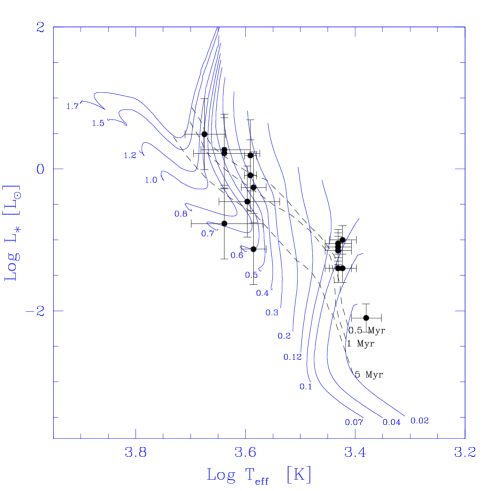
Figure 1: Location of the sample objects on the HR diagram. The evolutionary tracks (solid lines, labelled with the stellar mass) are from D’Antona and Mazzitelli (DM97 (1997)); dashed lines show isocrones at 0.5, 1 and 5 Myr, as marked.

2.2 Near-infrared spectroscopy

Near-infrared spectra in the J and K bands were obtained for all our targets using the ISAAC near-infrared camera and spectrograph at the ESO-VLT UT1 telescope. The observations were carried out in Visitor Mode on May 19-20, 2005. We used the 0.6 arcsec slit and the medium resolution grism that offered a $\sim$860 resolution across the wavelength 1.0-1.3 $\mu$m and $\sim$750 at 1.95-2.45 $\mu$m. The observing sequence was composed of a set of pairs of spectra with the target in different positions along the slit, to allow for an efficient and accurate sky subtraction. The on-source times varied from 30 to 60 min depending on target brightness and observing band (the J band observations were typically 30-40$\%$ shorter than the K band ones). Standard calibrations (flats and lamps) and telluric standards spectra were obtained for each observation. Wavelength calibration was performed using the lamp observations.

The Pa_β and Br_γ lines were observed as “simultaneously” as possible, to minimize the uncertainties due to the expected variability; to maintain a good temporal coherence of the observations of the two emission lines, every target was observed in a time sequence Br_γ–Pa_β–Br_γ. A complete observing cycle lasted about 2 hours.

The spectra were reduced using standard procedures in IRAF. After checking that the two Br_γ data sets were not significantly different (see §4.1), we combined all the exposures to obtain the final spectrum. The portion of the resulting spectra centered around the Pa_β and Br_γ lines is shown in Fig. 2.

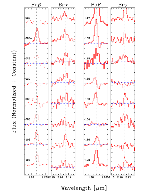
Figure 2: Pa$\beta$ (left panel) and Br$\gamma$ (right panel) spectra of the target objects. The observed fluxes have been normalized to the continuum near the line and shifted for an easier display.

3 Results

The equivalent widths of Pa_β and Br_γ were determined by fitting gaussian profiles to the spectra using standard iraf routines. The uncertainties were estimated from the uncertainties on the continuum location and from the equivalent width of noise spikes. We have checked that the equivalent width obtained by integrating the observed flux in excess of the continuum in a fixed wavelength range does not deviate from the values of the gaussian fit by more than 1$\sigma$.

In 13 objects Pa_β is clearly seen in emission, with equivalent width between $\sim 1$ and 6.5 Å. In 3 cases, the line is not seen and we report in Table 1 3$\sigma$ upper limits. In all objects, the emission lines are not resolved, with the exception of two of the sample TTS (ISO-Oph 163 and ISO-Oph 155), where we clearly detect red-shifted absorption. However, the resolution of our spectra is not suited for a study of the line profiles. Br_γ is generally weaker, and we have detected it in 8 objects only; in some cases, the equivalent widths have large uncertainties.

A comparison of the equivalent width of this paper with the measurements reported by Natta et al. (Nea04 (2004), Nea06 (2006)) shows the importance of measuring line ratios from spectra obtained simultaneously, as variations of factor of $\sim 2$ are possible. Of the three objects with non detected Pa_β, in two cases the current upper limits are consistent with our previous observations. In one case (ISO-Oph 164), however, Pa_β was clearly detected by Natta et al. (Nea04 (2004)), with an equivalent width of 0.8Å, significantly larger than our current upper limit (0.3 Å).

We compute line fluxes from the equivalent widths and the flux of the nearby continuum. We do not correct the equivalent width for underlying photospheric absorption, since the expected equivalent widths are small ($\mathbin{\lower 3.0pt\hbox{$\hbox to0.0pt{\raise 5.0pt\hbox{$\char 60\relax$}\hss}\mathchar 29208\relax$}}0.5$ Å, Wallace ate al. Wea00 (2000)) for objects with T_eff$\mathbin{\lower 3.0pt\hbox{$\hbox to0.0pt{\raise 5.0pt\hbox{$\char 60\relax$}\hss}\mathchar 29208\relax$}}5000$ K. As it was not possible to flux-calibrate the spectra, we estimated the continuum flux using the 2MASS values of the J and K magnitudes, proceeding as follows. The spectra were integrated over the 2MASS filter profiles and scaled to the measured 2MASS values. The resulting line fluxes were then corrected for extinction, according to the extinction law of Cardelli et al. Cea89 (1989) for $R_{V}$=4.2 and the values of A_J given in Table 1.

The ratio of the line fluxes Pa_β/Br_γ (R in the following) is given in Table 1, which gives also the 1$\sigma$ errors on R, computed taking into account only the errors on the measured equivalent widths and on the 2MASS photometry. They range from 3 to $\sim 40$%, in objects with very weak Br_γ. The possible systematic errors introduced by our flux calibration method and the extinction correction are discussed below.

Table 1, last column, gives the mass accretion rate $\dot{M}_{acc}$, computed from the luminosity of Pa_β, using the relation between L(Pa_β) and the accretion luminosity derived by Muzerolle et al. (Mea98b (1998)) and Natta et al. (Nea02 (2002)):

$$\log{L_{acc}/L_{\odot}}=1.36\,\log{L(P_{\beta})/L_{\odot}}+4$$ (1)

The mass accretion rate is then computed from L_acc:

$$\dot{M}_{acc}=L_{acc}\,R_{\star}/(GM_{\star})$$ (2)

The uncertainties on $\dot{M}_{acc}$ are dominated in most cases by uncertainties on the stellar parameters, and by the scatter of eq.(1) for very low luminosity objects. They can easily be of the order of one dex in Log $\dot{M}_{acc}$.

4 Discussion

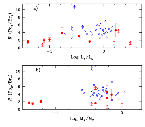
Figure 3: R is shown as a function of L_⋆ (Panel a) and of M_⋆ (Panel b) for the $\rho$-Oph objects; dots are measured values, arrows lower limits. Crosses plots R values for the Taurus TTS from Muzerolle et al. (Mea98b (1998)).

The values of R  span a rather large interval, varying from less than $2$ to $\mathbin{\lower 3.0pt\hbox{$\hbox to0.0pt{\raise 5.0pt\hbox{$\char 62\relax$}\hss}\mathchar 29208\relax$}}5$. We plot the values of R in Fig. 3 as a function of the luminosity of the central object and of its mass. Inspection of Fig. 3 shows that the 4 low luminosity (L_⋆$<0.1$L_⊙), low mass (M_⋆$\leq 0.06$M_⊙) objects with measured R (ISO-Oph 023, ISO-Oph 102, ISO-Oph 160, ISO-Oph 193) have R$\mathbin{\lower 3.0pt\hbox{$\hbox to0.0pt{\raise 5.0pt\hbox{$\char 60\relax$}\hss}\mathchar 29208\relax$}}2$. Values of R$\mathbin{\lower 3.0pt\hbox{$\hbox to0.0pt{\raise 5.0pt\hbox{$\char 62\relax$}\hss}\mathchar 29208\relax$}}3.5$ are only found in more massive objects, with M_⋆$\geq 0.4$ M_⊙.

In fig. 3, we have added to our objects the TTS in Taurus for which the ratio R has been measured by Muzerolle et al. (Mea98b (1998)). For better consistency, we have recomputed the R values from the line equivalent widths and A_J given by Muzerolle et al. (Mea98b (1998)), and 2MASS photometry. The differences with the values reported by Muzerolle et al. (Mea98b (1998)) are generally small.

The Taurus sample does not include any very low mass object and is limited to stars with M_⋆$\mathbin{\lower 3.0pt\hbox{$\hbox to0.0pt{\raise 5.0pt\hbox{$\char 62\relax$}\hss}\mathchar 29208\relax$}}0.25$ M_⊙, but it complements nicely our $\rho$-Oph data for TTS. In particular, one can see how, on one side, large values of R($\mathbin{\lower 3.0pt\hbox{$\hbox to0.0pt{\raise 5.0pt\hbox{$\char 62\relax$}\hss}\mathchar 29208\relax$}}3.5$) are observed only in higher mass objects, while on the other all the observed BDs have R$\mathbin{\lower 3.0pt\hbox{$\hbox to0.0pt{\raise 5.0pt\hbox{$\char 60\relax$}\hss}\mathchar 29208\relax$}}2$.

There are few higher mass objects with R$\sim 2$. One is ISO-Oph 002, which will be discussed in Sec.5. For the three Taurus objects with similarly low R (GI Tau, FS Tau and DG Tau), we note that the Taurus observations of Pa_β and Br_γ are not simultaneous, and line variability may affect by large factors the R value of individual objects. For example, the Pa_β equivalent width measured for GI Tau at two different epochs by Folha and Emerson (FE01 (2001)) varies by more than a factor of 2.

The low values of R  are particularly interesting, as we will dicuss in the following. However, before doing that, we need to examine the potential sources of error in the estimates of R, which may undermine the significance of our results.

4.1 Time variability

Line and continuum variability are well known in pre-main sequence stars of all masses. We have measured the two lines simultaneously, using an observational scheme Br_γ-Pa_β-Br_γ intended to minimize the effect of variability on R. In fact, it turns out that on the time scale of 1–2 hours, spanned by our observations, variability is not large, and the Br_γ equivalent widths measured before and after Pa_β are the same within the errors.

Note, however, that it has not been possible to calibrate our spectra photometrically, so that, in order to compute the line ratio R, we had to rely on magnitudes from the literature. 2MASS observations have been performed simultaneously in the three bands J,H,K, so that the values of R assigned to each object can be considered a correct, albeit “snapshot”, value, as long as there are no strong variations in the (J-K) colors of the stars. This seems to be indeed the case, as shown by Fig. 4, which compares the values of R obtained by using the J and K magnitudes measured by DENIS and by Barsony et al. (Bea97 (1997)), respectively, to those in Table 1, computed with 2MASS photometry. All sets of photometric observations have been obtained simultaneously in the J and K bands. The differences are always within 2$\sigma$; the five values of R  lower than $\sim 2$ remain low, while the R values of the order of 4 or larger remain so.

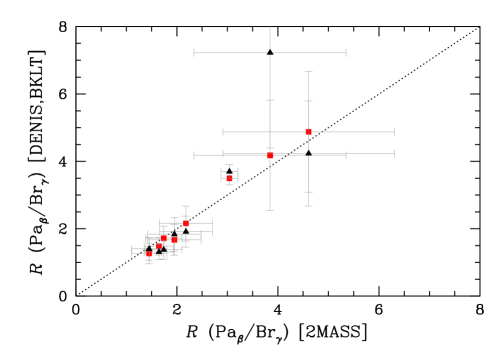
Figure 4: Comparison of R  using three different sets of near-IR photometry to derive the continuum flux at the line wavelengths. The horizontal axis shows R computed from the 2MASS photometry; on the vertical axis, the results obtained using DENIS (squares) and Barsony et al.(Bea97 (1997)) observations (triangles).

4.2 The extinction correction

The values of R  depend on the differential extinction between the J and K band. This extinction correction can be large in $\rho$-Oph objects, which are often very embedded, and introduces an additional uncertainty on R. In particular, underestimating A_J will result in values of R lower than the true ones, since R is proportional to $10^{0.22A_{J}}$ (for the adopted extinction law). Therefore, to push observed values of R from $\sim 2$ to $\sim 4$, one needs to increase the J band extinction by 1.37 mag.

Such an increase of A_J with respect to the values given in Table 1 is not consistent with the J, H, K spectra and photometry of the 4 low mass, low R objects (ISO-Oph 023, ISO-Oph 102, ISO-Oph 160 and ISO-Oph 193) studied by Natta et al. (Nea02 (2002)), who estimate uncertainties in A_J of $\sim$0.3 mag. In fact, independent estimates of A_V for two objects (ISO-Oph 030 and ISO-Oph 102) by Wilking et al. (Wea05 (2005)) result in values of A_J even lower than those adopted in this paper.

It is more difficult to estimate the A_J uncertainties for the 8 stars in our sample for which A_J is derived from the (J-H)-(H-K) colors. Luhman and Rieke (LR99 (1999)), using the Barsony et al. (Bea97 (1997)) photometry and a more complex scheme than the simpler one we have implemented, derive values of A_J for the 5 objects we have in common within 0.3 mag of our estimates. In one case (ISO-Oph 166) there is also in the literature an estimate of the extinction from optical spectra (Wilking et al. Wea05 (2005)), which agrees with our value within 0.1 mag.

In summary, although it is difficult to rule out the possibility of a large error on A_J in some individual object, we think it is unlikely that this can systematically affect our results. In particular, it does not seem possible to interpret all the low R values as due to an underestimate of the extinction.

5 Comparison with magnetospheric accretion models

The main aim of this work was to extend toward very low mass objects the comparison of the observed ratios Pa_β/Br_γ to the prediction of magnetospheric accretion models. In these models, gas is channeled from the disk onto the star along the lines of the stellar magnetic field and a shock forms where the accreting matter impacts on the stellar photosphere. The accretion luminosity is emitted mostly by the heated photosphere below the shock (the hot spots on the stellar surface), with the rest coming out from the pre-shock region. In accreting TTS, the heated photosphere and the pre-shock region are responsible for the continuum which veils the optical spectrum and for the strong ultraviolet continuum and line spectrum seen in these stars. The optical lines are believed to form not in the shocked region, which is very optically thick, but in the accreting columns, heated to roughly uniform temperatures (of order 8000 - 12000 K) not by the shock emission but by some alternative mechanism, possibly wave heating. These models have been very successful in explaining the complex phenomenon of TTS activity (e.g., Bouvier et al. Bou_PPV (2006) and references therein).

In the magnetospheric accretion models, for fixed stellar parameters and field geometry, R depends on the mass accretion rate Macc and temperature of the accreting gas. As mentioned, the gas temperature is not computed self-consistently, but has been constrained by fitting different lines of various atomic species (see Muzerolle et al. Mea01 (2001)). Within these constraints, the infrared lines are thermalized for the gas densities expected for average values of $\dot{M}_{acc}$. Both the line luminosities and R do not change with decreasing density until $\dot{M}_{acc}$$\mathbin{\lower 3.0pt\hbox{$\hbox to0.0pt{\raise 5.0pt\hbox{$\char 60\relax$}\hss}\mathchar 29208\relax$}}10^{-8}$ M_⊙/yr, at which point the line optical depth goes below unity first at Br_γ and then Pa_β  and R quickly increases to very large values. There are additional free parameters, namely the exact location of the base of the accreting region and its inclination to the line of sight, which, however, do not change this basic picture.

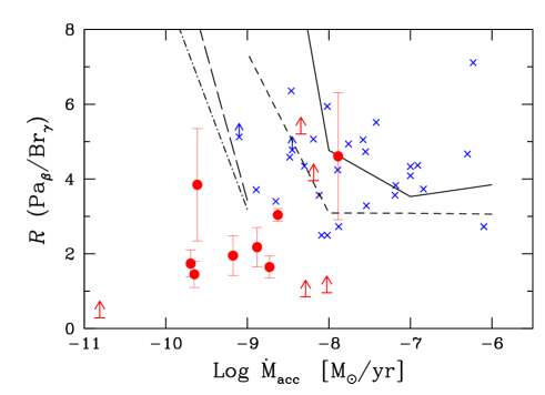
Figure 5: R as a function of $\dot{M}_{acc}$ for the $\rho$-Oph objects; dots show actual measurements, arrow lower limits. $\dot{M}_{acc}$ has been derived from the Pa_β luminosity, as described in the text. Crosses show the location of Taurus TTS (from Muzzerolle et al. Mea98b (1998)). The different lines show the predictions of magnetospheric accretion models which roughly fit the UV veiling and the H_α profiles. Solid and short-dashed lines show models for TTS (M_⋆=0.5 M_⊙, R_⋆=2 R_⊙) with inner and outer magnetosphere boundaries at the disk of 2.2–3 R_⋆(solid) and 2.8–3 R_⋆(short-dashed). The temperature of the accreting gas increase from 7000 K (for $\dot{M}_{acc}$= $10^{-6}$ M_⊙/yr) to 12000 K for $\dot{M}_{acc}$=$10^{-9}$ M_⊙/yr(see Muzerolle et al. Mea01 (2001) for details). The other two lines show models for typical BD parameters (M_⋆=0.05 M_⊙, R_⋆=0.5 R_⊙), magnetosphere boundaries 2.2–3 R_⋆, temperature of 12000 K (long-dashed) and 10000 K (dot-dashed), respectively.

The predictions of magnetospheric accretion models are compared to our results in Fig. 5, which shows that the models reproduce quite well the bulk of the R values in the Taurus TTS (Muzerolle et al. Mea01 (2001)).

The situation is different for the $\rho$-Oph BDs, which have much lower $\dot{M}_{acc}$ than TTS (e.g., Muzerolle et al. Mea03 (2003), Mea05 (2005); Natta et al. Nea04 (2004); Mohanty et al. Subu05 (2005)). Fig. 5 shows model prediction for stellar parameters typical of BDs and $\dot{M}_{acc}$$\leq 10^{-9}$ M_⊙/yr. The gas temperature required to fit intensity and profiles of H_α is T$\mathbin{\lower 3.0pt\hbox{$\hbox to0.0pt{\raise 5.0pt\hbox{$\char 62\relax$}\hss}\mathchar 29208\relax$}}8000$ K. In these models R $\sim 3.5$ for $\dot{M}_{acc}$$=10^{-9}$ M_⊙/yr, and increases rapidly with decreasing $\dot{M}_{acc}$. It is clear that they cannot reproduce the observed low R values of the $\rho$-Oph BDs.

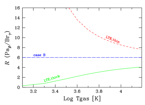
Figure 6: R is plotted as a function of the gas temperature T_gas for three textbook cases. The solid line shows the case of optically thick lines with LTE level population; the dashed line the case of LTE, optically thin lines. The dash-dotted line the value of R for case B recombination.

R$\sim 2$ is obtained if the lines form in a cold, optically thick gas. This is shown in Fig. 6, which plots the R values expected as a function of the gas temperature $T$ in different physical situations. The line at R$\sim 6$ shows the predictions of Case B, i.e., the value of R when the lines are optically thin and the level population is dominated by radiative cascade from the continuum. If the hydrogen levels from which the near-IR lines originate ($n\geq 3$) are in LTE, the dependence of R on the temperature is different for optically thin and optically thick lines. When the lines are optically thin, R$\mathbin{\lower 3.0pt\hbox{$\hbox to0.0pt{\raise 5.0pt\hbox{$\char 62\relax$}\hss}\mathchar 29208\relax$}}8$ for temperature $T\sim 10000$K and increases for decreasing $T$ (dashed line). On the contrary, when the lines are optically thick, R decreases for decreasing temperature, from $\sim 4$ for $T\mathbin{\lower 3.0pt\hbox{$\hbox to0.0pt{\raise 5.0pt\hbox{$\char 62\relax$}\hss}\mathchar 29208\relax$}}$ 8000 K to $\sim 2$ for $T\sim 3500$ K.

If indeed the lines are thermalized, the size of the emitting region can be estimated from Fig. 7, which plots the luminosity of Pa_β  as a function of R for the Ophiuchus and Taurus sample. The three curves show the location of thermalized, optically thick IR line emission for different values of the projected area of the emitting region, from $2\times 10^{22}$ to $2\times 10^{20}$ cm² and a FWHM line width of 100 km s^-1. The four BDs (ISO-Oph 23, ISO-Oph 102, ISO-Oph 160 and ISO-Oph 193) with R$\sim 2$, are well fitted by black body emission at T$\sim 3500$ K and area $\sim 2\times 10^{21}$ cm². This is a small fraction of the projected photospheric surface, varying between $\sim 6$ and 15% in the four objects. Note that at the resolution of our data ($\sim 350$ km/s) the BDs lines are not resolved; as the Pa_β flux is proportional to the product of the emitting area times the line width, larger or smaller values of the latter will result in a proportionally smaller or larger values of the emitting surface.

These properties (i.e., temperature higher than T_eff, small covering fraction, high optical depth) remind those of the hot spots caused by magnetospheric accretion on the stellar surface of classical TTS.

Models of the accretion shock have been computed by Calvet and Gullbring (CG98 (1998)) for the parameters typical of TTS. They showed that the emission originates from three different regions, the pre-shock accreting columns, the post-shock gas and the heated photosphere below the shock (the hot spot). The physical properties of these regions are controlled by the energy flux of the accretion flow $\cal F$:

$${\cal F}=9.8\times 10^{10}\>{\rm erg\,cm^{-2}\,s^{-1}}\>\Big{(}{\rm{{\dot{M}_{acc}}\over{10^{-8}\,M_{\odot}\,yr^{-1}}}}\Big{)}$$

$$\Big{(}{\rm{{M_{\star}}\over{0.5M_{\odot}}}}\Big{)}\>\>\Big{(}{\rm{{R_{\star}}\over{2R_{\odot}}}}\Big{)}^{-3}\>\>\Big{(}{{f}\over{0.01}}\Big{)}^{-1}$$ (3)

where $f$ is the fraction of the stellar surface covered by the accretion spots. In TTS $\cal F$ ranges between $3\times 10^{10}$ and $10^{12}$ erg cm^-2 s^-1; with these values of $\cal F$, the heated photosphere is very optically thick, and emits a continuum spectrum with temperatures much higher than T_eff, which accounts for the UV veiling. The models are quite complex and cannot be simply scaled to the BD parameters. However, we note that the energy flux of the accretion flow in the four $\rho$-Oph BDs is ${\cal F}\sim 5\times 10^{7}-5\times 10^{8}$ erg cm^-2 s^-1, much lower than in TTS (see Fig. 8). From the Calvet and Gullbring models, one expects that both the enhancement of the temperature with respect to the undisturbed photosphere, and the depth of the affected region decreases with ${\cal F}$, so that it seems possible to obtain line emission with the required properties from the heated photosphere.

Fig. 8 plots the observed values of R as a function of ${\cal F}$ for Taurus and $\rho$-Oph objects. For Taurus, we have computed ${\cal F}$ from the accretion rates, stellar parameters and the surface coverage of the accretion columns given by Calvet and Gullbring (CG98 (1998)), using their eq.(11). For the $\rho$-Oph objects, we take the temperature and the area of the emitting region from the location of the object in Fig 7, assuming black body emission. This is possible for the 6 objects with R$\mathbin{\lower 3.0pt\hbox{$\hbox to0.0pt{\raise 5.0pt\hbox{$\char 60\relax$}\hss}\mathchar 29208\relax$}}3.5$. One can see that 5 of them (the 4 BDs and ISO-Oph 002), which have R$\sim 2$, also have ${\cal F}$ much smaller than the Taurus TTS. The sixth object (ISO-Oph 117) has R$\sim 3.5$ and ${\cal F}$ similar to the lowest values of Gullbring & Calvet. The correlation between R and ${\cal F}$ stops at ${\cal F}\sim 10^{10}$; for higher ${\cal F}$, all the objects have similar values of R.

We propose a scenario where for high $\dot{M}_{acc}$ the optical and infrared continuum emission of the heated photosphere is optically thick and all the hydrogen lines (optical and IR) observed in emission originate from the accreting columns of gas. When $\dot{M}_{acc}$ decreases below a threshold value the continuum emission of the hot spots becomes optically thin and the lines appear in emission; at the same time, the density of the accreting gas decreases and its line spectrum gets weaker. As a consequence, lines of lower optical depth have an increasing contribution from the shocked regions. In BDs, this region dominates the emission of the near-IR hydrogen lines, while optical lines, such as H_α  still originates mostly in the accreting columns of gas. If this will be confirmed by further observations and by model calculations, the IR hydrogen lines may provide a measurement of $\dot{M}_{acc}$ in BDs in analogy to continuum veiling in TTS, less model-dependent than the H_α profiles used so far.

A similar picture is suggested by Edwards et al. (Eea06 (2006)), who obtained high resolution profiles of Pa_γ in classical Taurus TTS. They find that the Pa_γ width correlates with the veiling at 1 $\mu$m, which may be a tracer of $\dot{M}_{acc}$. The width of lines forming in the accreting gas columns should not depend on $\dot{M}_{acc}$, for fixed stellar and disk parameters, and Edwards et al. argue that their results can be understood if the relative contribution of the accretion shock to the Pa_γ emission increases as $\dot{M}_{acc}$  decreases.

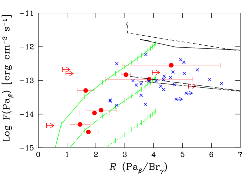
Figure 7: Pa_β flux versus R for Ophiuchus (dots and arrows) and Taurus (crosses). The three curves ending at R$\sim 4$ show the LTE, optically thick line emission case. Along each line, the temperature increases from 1000 K to 15000 K, in steps of 1000 K (tick marks); the first mark corresponds to T=2000 K on the top curve, to T=3000 K for the middle curve and to T=5000 K for the lowest one. Note that the values of R depend on T only. Each curve corresponds to a different value of the emitting area, $2\times 10^{22}$ cm² (solid line), $2\times 10^{21}$ cm² (long-dashed line) and $2\times 10^{20}$ cm² (dotted line) from top to bottom, respectively. In all cases, we have assumed a Pa_β FWHM of 100 km s^-1; the Pa_β flux is proportional to the emitting area times the line width. Magnetospheric accretion models (same as in Fig. 5) are shown by the roughly horizontal lines (same as Fig. 5). Slightly lower values of the gas temperature in the accreting columns will give lower value of F(Pa_β), while still roughly fitting the observations. Note, however, that in no case R$<3$.

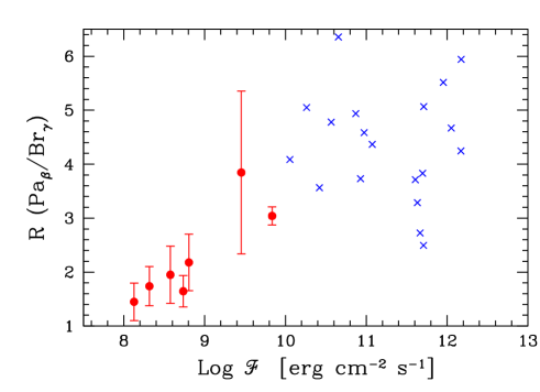
Figure 8: R values plotted against the energy flux of the accretion flow $\cal F$. Estimates for the $\rho$-Oph objects (dots) have been derived from their measured $\dot{M}_{acc}$, stellar parameters and an emitting area estimated by tring heir location on the F(Pa_β)–R with the predictions of LTE, optically thick emission (Fig. 7); two objects (ISO-Oph 037 and ISO-Oph 163) with R$\mathbin{\lower 3.0pt\hbox{$\hbox to0.0pt{\raise 5.0pt\hbox{$\char 62\relax$}\hss}\mathchar 29208\relax$}}4.5$ no estimate of $\cal F$ was possible. The values for Taurus TTS have been computed from $\dot{M}_{acc}$ and stellar parameters given by Muzerolle et al. (Mea98b (1998)) and the fraction fo stellar surface covered by the accretion spots computed by Calvet and Gullbring (CG98 (1998)). In all cases we have used eq.(11) of Calvet and Gullbring (CG98 (1998)).

6 Summary and conclusions

This paper presents the results of simultaneous measurements of Pa_β and Br_γ in a sample of 16 objects in the $\rho$-Oph region. We measure the ratio of the line fluxes R=Pa_β/Br_γ in 8 objects, 4 of which are spectrally confirmed very low mass stars or brown dwarfs (BDs in this paper). In 5 other cases we could not detect Br_γ, and we estimate lower limits to R.

The 4 BDs all have R$\sim 2$; of the other stars, one has R$\sim 2$, while the others have R$\geq 3.5$, similar to the values measured in accreting TTS in Taurus (Muzerolle et al. Mea98b (1998)). We discuss the measured R values in the context of magnetospheric accretion models where hydrogen recombination lines form in the accreting columns of gas that connect the disk to the star. The gas is heated to temperatures of $\sim 8000-12000$K, and the predicted values of R are in all cases $\geq 3.5$. The low R observed in the $\rho$-Oph BDs cannot be explained by these models.

We propose that, at the low $\dot{M}_{acc}$ typical of the BDs, the hydrogen near-IR lines form instead in the shock-heated stellar photosphere, and discuss how it is possible to produce in these regions the required low temperature and high optical depths in the line (but not in the continuum) that will result Pa_β and Br_γ emission with in R$\sim 2$. This possibility needs to be investigated with the help of models similar to those of Calvet and Gullbring (CG98 (1998)), which compute the emission of the various components of magnetospheric accretion (accreting column, shock-heated photosphere and post-shock gas) for low $\dot{M}_{acc}$ values and the parameters typical of BDs.

Finally, we note that the luminosity of the hydrogen IR recombination lines has been extensively used to derive the accretion rate in large sample of objects, especially when UV veiling could not be measured (e.g., Natta et al. Nea06 (2006)). The calibration of the line luminosity – accretion relationship has been derived empirically, using objects with L_acc measured independently from veiling or (for very low mass objects) from the H_α profiles, not from models. The results of this paper, which suggests that the IR lines may not necessarily form in the accreting columns, do not weaken their reliability as a tool to measure the accretion rate. In fact, if they form in the accretion spots, they may provide a measurement of $\dot{M}_{acc}$ in BDs in analogy to continuum veiling in TTS, less model-dependent than the H_α profiles used so far.

Appendix A Spectral classification of the Ophiuchus objects

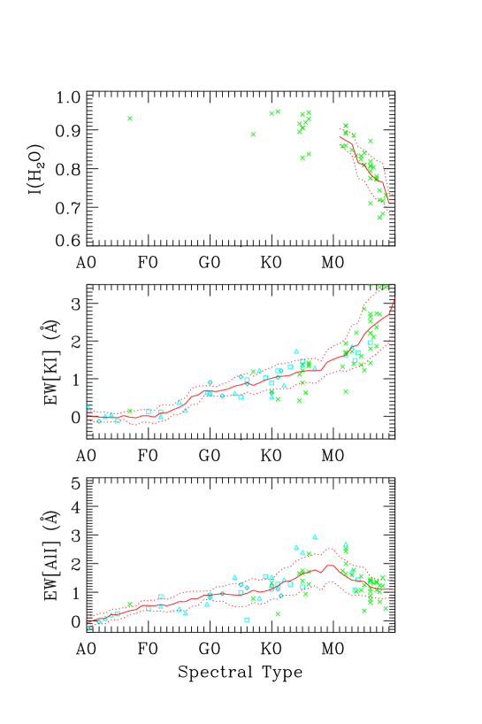
Figure 9: Run of the main spectral indices used for the spectral classification as a function of the spectral type. The top panel shows an index that measures the water vapour absorption at the red end of the J-band, the middle and bottom panels show the equivalent width of the [KI] and [AlII] lines within the J-band. Open squares, triangles and diamonds show the values of the [KI] and [AlII] equivalent widths computed for the giants (luminosity class III), dwarfs (V) and subgiants (IV) of Wallace et al. (2000), respectively. Crosses show the values of the same indices for the objects with known spectral type in Ophiuchus. The solid lines are smoothed averages of the measured points, the dotted lines show the dispersion within the smoothing interval ($\pm 3$ subclasses); they have been used to estimate the spectral type range for our target stars from the measured indices.

Many of our targets do not have a reliable spectral classification in the literature, others have been classified using a variety of different methods, from low resolution optical, to K-band or high resolution infrared spectroscopy. We attempted to use our J-band spectra to estimate in a uniform fashion the spectral types of all objects in our sample. The J-band was chosen because at this wavelength the photosphere dominates the emission even for Class II objects and the effect of veiling from the disk infrared excess emission is thus limited, especially in the BDs.

We computed the equivalent widths for a number of photospheric lines, following Wallace (Wea00 (2000)). Due to the lower resolution of our spectra, we needed to adjust the limits for the computation of the equivalent widths given in Table 3 of Wallace et al.; thus, we recomputed the values of the equivalent widths for all spectra in their list. We also computed the equivalent width values for all $\rho$-Oph Class II objects in our Natta et al. (Nea06 (2006)) sample with a solid spectral classification in the literature, mainly from Luhman & Rieke LR99 (1999) or from Natta et al. Nea02 (2002). To improve the possibility of a good spectral classification at late types we also defined a spectral index based on the water absorption features at the red edge of the band, in a similar fashion as Testi et al. (Tea01 (2001)). This index was computed only for the $\rho$-Oph Class II objects with known spectral type. In Figure 9, we show the run of the equivalent widths of [AlII] and [KI] and the water index as a function of the known spectral type. For late spectral types (K-M) a combination of the various indices may allow a reasonable classification within a few subclasses, at earlier spectral types the correlations of the indices with the spectral type flattens significantly and the classification is more uncertain (if at all possible).

Using the equivalent widths and the water index, for each of the stars in our sample we derived a range of possible spectral types compatible with the measured values. These are reported in Table 2 along with the spectral types found in the literature. In general our estimate of the spectral type is consistent with the values found in the literature. Following this comparison, for each target, we adopt a fiducial spectral type that is used throughout this paper to derive the stellar parameters (Column 9). For the very low mass stars and brown dwarfs studied in Natta et al. (Nea02 (2002)) we adopt their spectral type as our spectral type range is essentially based on the water index and is more uncertain than the classification made using the complete near infrared spectrum. For these objects the adopted type is always within the range we derive here, with the exception of $\rho$Oph-ISO 193, for which an earlier type (by 2 subclasses) is possible. For the stellar objects, the adopted spectral type is at the center of the range derived here, and it is usually consistent with the estimates in the literature. Some of the objects, however, have very uncertain spectral classification, this is reflected in the larger uncertainties in the effective temperature estimate used in Sect. 2.1 and Fig. 1.

Table 2: Line indexes and derived spectral types. Column 1: name of object; 2, 3, 4: H₂O, KI and AlI indexes measured from this paper spectra; 5, 6, 7: same from Natta et al. (Nea06 (2006)) J-band spectra; column 8: spectral type range; column 9: adopted spectral type; column 10–13: spectral types from Natta et al. (Nea02 (2002)), Luhman and Rieke (LR99 (1999)), Wilking et al. (Wea05 (2005)) and Doppmann et al. (Dea05 (2005)), respectively; column 14: other source names.

Name	H2O	K I	Al I	H2O	K I	Al I	ST	ST	ST	ST	ST	ST	Other Names
	This Paper			Nea06			range	adopted	Nea02	LR99	Wea05	Dea05
ISO-Oph 002a	0.95	1.9	2.1	0.88	1.8	1.6	K8–M2	M0	–	–	–	–	B162538-242238
ISO-Oph 023	0.75	1.5	0.5	0.78	2.7	1.1	M4–M9	M7	M7	–	–	–	SKS1
ISO-Oph 030	0.79	2.2	1.2	0.82	2.2	1.4	M4-M8	M6	M6	M5-M6	M5.5	–	GY5
ISO-Oph 033	0.71	2.7	0.7	0.73	3.4	0.5	M7–M9	M8.5	M8.5	–	–	–	GY11
ISO-Oph 037	0.99	1.0	1.9	0.92	1.7	2.5	K0–K9	K5	–	K-M	–	K9	LFAM3/GY21
ISO-Oph 083	0.93	1.9	2.0	0.92	1.7	1.4	K8–K9	K9	–	–	–	–	BL162656-241353
ISO-Oph 102	0.81	2.1	1.1	0.80	2.7	1.1	M3–M6	M6	M6	–	M5.5	–	GY204
ISO-Oph 105	0.93	1.5	1.6	0.92	1.1	1.8	K8–M0	K9	–	K5-M2	–	M3	WL17/GY205
ISO-Oph 115	0.85	0.8	1.2	0.88	1.0	2.1	K9–M2	M0	–	–	–	–	WL11/GY229
ISO-Oph 117	0.93	1.4	1.3	0.86	1.2	2.4	K2–M3	K8	–	–	–	–	GY235
ISO-Oph 155	0.96	0.9	1.4	0.94	0.8	1.3	K0–K5	K3	–	K5-M2	–	–	GY292
ISO-Oph 160	0.81	2.2	1.2	0.81	2.6	1.4	M3–M8	M6	M6	–	–	–	B162737-241756
ISO-Oph 163	0.96	1.2	1.6	0.91	1.3	1.8	K0–K8	K5	–	K5-M2	–	–	IRS49/GY308
ISO-Oph 164	0.70	3.0	1.0	0.71	3.5	0.7	M7–M9	M6	M6	–	M3-M5	–	GY310
ISO-Oph 166	0.93	1.6	2.1	0.91	1.4	1.8	K2–K8	K5	–	K6-M2	K0	–	GY314
ISO-Oph 193	0.86	1.4	1.3	0.87	1.4	0.8	M1–M4	M6	M6	–	–	–	B162812-241138

References

- (1) Alencar S.H.P., Basri G. 2001, AJ 119, 1881
- (2) Barsony M., Kenyon S.J., Lada E.A., Teuben P.J. 1997, ApJS 112, 109
- (3) Bontemps S., André Ph., Kaas A.A., et al. 2001, A&A 372, 173
- (4) Bouvier J., Alencar S.H.P., Harries T.J., Johns-Krull C.M., Romanova M.M. 2006, in Protostars & Planets V, Eds. B. Reipurth, D. Jewitt, and K. Keil, University of Arizona Press (Tucson), in press
- (5) Calvet N., Gullbring E. 1998, ApJ 509, 802
- (6) Calvet N., Muzerolle J., Briceño C., Hernàndez J., Hartmann L., Saucedo J.L., Gordon K.D. 2004, ApJ 128, 1294
- (7) Cardelli J.A., Clayton G.C., Mathis J.S. 1989, ApJ 345, 245
- (8) D’Antona F., Mazzitelli I. 1997, Mem.S.A.It. 68, 807
- (9) Doppmann G.W., Greene T.P., Covey K.R., Lada C.J. 2005, AJ 130, 1145
- (10) Edwards S., Hartigan P., Ghandour L., Andrulis C. 1994, AJ 108, 1065
- (11) Edwards S., Fischer W., Hillenbrand L., Kwan J. 2006, ApJ 646, 319
- (12) Folha D.F.M., Emerson J.P. 2001, A&A 365, 90
- (13) Garcia Lopez R., Natta A., Testi L., Habart E., 2006, å, submitted
- (14) Gullbring E., Hartmann L., Briceño C., Calvet N. 1998, ApJ 492, 323
- (15) Hartmann L., Hewett R., Calvet N. 1994, ApJ 426, 669
- (16) Kenyon S.J., Hartmann L. 1995, ApJS 101, 117
- (17) Kenyon S.J., Lada E.A., Barsony M. 1998, AJ 115, 252
- (18) Lamzin S.A. 1995, å295, 20
- (19) Lamzin S.A. 1998, ARep 42, 322
- (20) Luhman K.L., Rieke G.H. 1999, ApJ 525, 440
- (21) Meyer M.R., Calvet N., Hillenbrand L.A. 1997, AJ 114, 288
- (22) Mohanty, S., Jayawardhana, R., Basri, G. 2005, ApJ, 626, 498
- (23) Muzerolle J., Calvet N., Hartmann L. 1998, ApJ 492, 743
- (24) Muzerolle J., Hartmann L., Calvet N. 1998, AJ 116, 2965
- (25) Muzerolle J., Calvet N., Hartmann L. 2001, ApJ 550, 944
- (26) Muzerolle J., Calvet N., Briceño C., Hartmann L., Hillenbrand L. 2000, ApJ 535, L47
- (27) Muzerolle J., Hillenbrand L., Calvet N., Briceño C., Hartmann L. 2003, ApJ 592, 266
- (28) Muzerolle J., D’Alessio P., Calvet N., Hartmann L. 2004, ApJ 617, 406
- (29) Muzerolle J., Luhman K.L., Briceño C., Hartmann L., Calvet N. 2005, ApJ 625, 906
- (30) Natta A., Testi L., Comerón F., Oliva E., D’Antona F., Baffa C., Comoretto G., Gennari S., 2002, A&A 393, 597.
- (31) Natta A., Testi L.,Muzerolle J., Randich S., Comerón F., Persi P. 2004, A&A 424, 603
- (32) Natta A., Testi L., Randich S. 2006, A&A 452, 245
- (33) Testi L., D’Antona F., Ghinassi F., Licandro J., Magazzú A. et al. 2001, ApJ 552, L147
- (34) Wallace L.W., Meyer M.R., Hinkle K., Edwards S. 2000, ApJ 535, 325
- (35) Wilking B.A., Meyer M.R., Robinson J.G., Greene Th. 2005, AJ 130, 1733