The evolution of the near-IR galaxy Luminosity Function and colour bimodality up to ${\bf z\simeq 2}$ from the UKIDSS Ultra Deep Survey Early Data Release

Abstract

We present new results on the cosmological evolution of the near-infrared galaxy luminosity function, derived from the analysis of a new sample of $\sim 22,000$  $K_{\rm AB}$$\leq 22.5$ galaxies selected over an area of 0.6 square degrees from the Early Data Release of the UKIDSS Ultra Deep Survey (UDS). Our study has exploited the multi-wavelength coverage of the UDS field provided by the new UKIDSS WFCAM $K$ and $J$-band imaging, the Subaru/XMM-Newton Deep Survey and the Spitzer-SWIRE Survey. The unique combination of large area and depth provided by this new survey minimises the complicating effect of cosmic variance and has allowed us, for the first time, to trace the evolution of the brightest sources out to $z\simeq 2$ with good statistical accuracy.

In agreement with previous studies we find that the characteristic luminosity of the near-infrared luminosity function brightens by $\simeq 1$ magnitude between $z=0$ and $z\simeq 2$, while the total density decreases by a factor $\simeq 2$. Using the rest-frame $(U-B)$ colour to split the sample into red and blue galaxies, we confirm the classic luminosity-dependent colour bimodality at $z\raisebox{-3.69899pt}{~{}\shortstack{$<$ \\ [-0.07cm] $\sim$}}~{}1$. However, the strength of the colour bimodality is found to be a decreasing function of redshift, and seems to disappear by $z\mathrel{\hbox to0.0pt{\lower 3.0pt\hbox{$\sim$}\hss}\raise 2.0pt\hbox{$>$}}1.5$. Due to the large size of our sample we are able to investigate the differing cosmological evolution of the red and blue galaxy populations. It is found that the space density of the brightest red galaxies ($M_{K}\leq-23$) stays approximately constant with redshift, and that these sources dominate the bright-end of the luminosity function at redshifts $z\raisebox{-3.69899pt}{~{}\shortstack{$<$ \\ [-0.07cm] $\sim$}}~{}1$. In contrast, the brightening of the characteristic luminosity and mild decrease in space density displayed by the blue galaxy population leads them to dominate the bright-end of the luminosity function at redshifts $z\raisebox{-3.69899pt}{~{}\shortstack{$>$ \\ [-0.07cm] $\sim$}}~{}1$.

1 INTRODUCTION

The potential of deep near-infrared observations to measure the cosmological evolution of the stellar mass of galaxies has long been understood (e.g. Lilly & Longair 1984; Dunlop et al. 1989; Glazebrook et al. 1995; Cowie et al. 1996). Now, with the advent of wide-field near-infrared detectors, this potential has begun to be realized, and several deep infrared-based studies supported by spectroscopic and/or photometric redshift information have recently been completed (e.g. Cimatti et al. 2002; Pozzetti et al. 2003; Dickinson et al. 2003; Drory et al. 2003; Fontana et al. 2004; Glazebrook et al. 2004; Caputi et al. 2006; Drory et al. 2005).

A key aim of this work is the determination of the cosmological evolution of the $K$-band galaxy luminosity function (LF), the present-day form of which is now reasonably well established (Cole et al. 2001; Kochanek et al. 2001). The most recent studies have been deep enough, and have been armed with sufficient redshift information to attempt to trace this evolution out to $z=2-3$. The results indicate a substantial brightening in characteristic magnitude from $z=0$ up to $z=2-3$ along with a simultaneous decrease in galaxy number density (see e.g. Caputi et al. 2006; Saracco et al. 2006). A similar combination of luminosity and density evolution has also been observed in the optical LF (e.g. Lilly et al 1995; Poli et al. 2003; Gabasch et al. 2004; Giallongo et al. 2005).

However, even these most recent deep near-infrared surveys have still only covered relatively small areas of sky (from a few $\rm arcmin^{2}$ in the Hubble Ultra Deep Field to several hundred $\rm arcmin^{2}$ in the Great Observatories Origins Deep Survey (GOODS)) and are hence existing results on the evolving LF are still potentially heavily affected by cosmic variance. In this paper we exploit the order-of-magnitude improvement in areal coverage (0.6 sq. deg.) provided by the the UKIRT Infrared Deep Sky Survey (UKIDSS; Lawrence et al. 2006) Ultra Deep Survey (UDS) to constrain the evolution of the near-infrared LF and the colour bimodality up to $z\mathrel{\hbox to0.0pt{\lower 3.0pt\hbox{$\sim$}\hss}\raise 2.0pt\hbox{$>$}}2$.

The rest of this paper is structured as follows. In Section 2 we summarize the main properties of the datasets used in this work. Then, in Section 3 we describe in detail how our new $K$-band galaxy sample has been constructed and cleaned, and describe the method we have developed for the estimation of redshifts from the available multi-band photometry. In Section 4 we assess and discuss the reliability of our photometric redshift estimates and in Section 5 we derive the near-infrared LF. The evolution of the colour bimodality is presented in Section 6 while in Section 7 we derive separate LFs for the populations of red and blue galaxies. Our conclusions are presented in Section 8.

Throughout this paper all magnitudes are given in the AB system (Oke & Gunn 1983) and we have adopted a background cosmology with $\Omega_{\rm M}=0.3$, $\Omega_{\Lambda}=0.7$ and $H_{0}=70~{}{\rm km~{}s^{-1}}$.

2 The Data-sets

The data exploited in this paper cover a large range in wavelengths from the optical to the mid-infrared and have been obtained by combining three different surveys. The optical data were taken with the Subaru Telescope as part of the Subaru/XMM-Newton Deep Survey (Sekiguchi et al. 2005), the near-infrared data form part of the early-data release (Dye et al. 2006) of the UKIRT Infrared Deep Sky Survey (Lawrence et al. 2006) and mid-infrared data have been obtained with the Spitzer satellite as part of the Spitzer wide-area infrared extragalactic (SWIRE) survey (Lonsdale et al. 2003; 2004). In this Section the main properties of these three surveys are briefly outlined.

2.1 The Subaru/XMM-Newton Deep Survey

The Subaru/XMM-Newton Deep Survey (SXDS) is a multi-wavelength survey covering an area of $\sim 1.3$ square degrees. This area, centred on RA=02:18:00 and Dec=$-$05:00:00 (J2000), benefits from deep optical imaging undertaken with Suprime-Cam (Miyazaki et al. 2002) on Subaru. The 5 over-lapping Suprime-Cam pointings provide broad band photometry in the $BVRi^{\prime}z^{\prime}$ filters to typical $5\sigma$ depths of $B=27.5$, $V=26.7$, $R=27.0$, $i^{\prime}=26.8$ and $z^{\prime}=25.9$ (within a $2$-arcsec diameter aperture).

The X-ray observations of this field were obtained with the XMM-Newton satellite and comprise 400 ksec exposures in 7 contiguous fields to a depth of $\rm\sim few\;10^{-15}\;erg\;cm^{-2}\;s^{-1}$. The field also has deep 1.4 GHz radio observations from the VLA (Simpson et al. 2006a) and $\rm 850\mu m$ sub-mm observations from SCUBA as part of the SHADES survey (Mortier et al. 2005; Coppin et al. 2006).

2.2 The UKIDSS Ultra Deep Survey

The central region of the SXDS is being observed at near-infrared wavelengths with the Wide-Field Camera (WFCAM - Casali et al. 2006, in preparation) on UKIRT, as part of the UKIDSS Ultra Deep Survey (UDS). The UDS is the deepest of the five surveys that constitute the UKIRT Infrared Deep Sky Survey (UKIDSS - Lawrence et al. 2006) and ultimately aims to cover 0.8 square degrees to a depth $J_{AB}=26$, $H_{AB}=25.4$ and $K_{AB}=25$ over a seven year period. AB magnitudes in the UDS have been obtained by using calibrations from Hewett et al. (2006). For the present study the first twelve hours of $J,K$ imaging, which constitute the early data release (EDR – Dye et al. 2006) of the UDS, have been used. These data reach $5\sigma$ limits of $J_{AB}=22.5$ and $K_{AB}=22.5$ within a $2$-arcsec diameter aperture. The details of the stacking and catalogue extraction are fully described in Foucaud et al. (2007).

2.3 The SWIRE survey

The Spitzer wide-area infrared extragalactic survey (SWIRE – Lonsdale et al. 2003; 2004) is a large Spitzer Legacy program which covers seven high-latitude fields with a total area of $\sim 65$ sq. deg. In this paper we exploit the Spitzer observations covering $9.1$ sq. deg. in the XMM-LSS field which cover the SXDS field. The source catalogue based on the data release 2 (Surace et al. 2005) includes sources with detections at IRAC $\rm 3.6\mu m$ and $\rm 4.5\mu m$ wavelengths to a depth of $\rm\sim 10\mu Jy$ $SNR\simeq 10$ in both bands ( $\simeq 21.4$ in AB magnitudes).

Figure 1: Photometric redshift plotted versus spectroscopic redshift for $\sim 1100$ sources in the UDS sample with available spectroscopic redshift determinations (Yamada et al. 2005; Akiyama et al. in preparation; Smail et al. in preparation; Simpson et al. 2006a). Left panel shows the comparison for sources with $K_{AB}<22$ while the comparison for fainter sources with $K_{AB}\geq 22$ is presented in the right panel. The small insets in both panels show the distribution of the $\Delta z/(1+z)$. The agreement is remarkably good with a mean value of $\Delta z/(1+z)$ of 0.006, and a standard deviation $\sigma=0.04$, excluding the clear outliers (see text for details).

3 The UDS-galaxy sample

Exploiting the multi-wavelength coverage and the large area provided by the combination of the surveys described in the previous Section, we aim to derive a complete sample of $K$-band selected galaxies, with photometrically estimated redshifts. Only sources with  $K_{\rm AB}$$\leq 22.5$ have been included in the sample, which is the $5\sigma$ magnitude limit of the EDR data (see Section 2.2). The completeness at the limiting magnitude has been estimated to be above $70$% with a fraction of spurious detections less than 1% (Foucaud et al. 2007). In order to have an homogeneous multi-wavelength coverage for each object we use optical and near-infrared photometry computed in a 2” diameter apertures PSF corrected to total. The consistent image quality of optical and near-infrared data ($0.7<\rm FWHM<0.8$ arcsec) means that the differential aperture corrections between bands are small ($\leq 0.1$ mag). The Spitzer SWIRE photometry is in 2.8” diameter apertures PSF corrected to total (see Surace et al. 2005).

Due to a small shift of the UDS field centre during the first year of observations, the current $J,K$ photometry in the EDR is uniform only over an area of $0.6$ square degrees. Therefore, in order to obtain homogeneous coverage over all the optical and near-IR spectral range, we have limited our sample to include only sources in the central $0.6$ square degree area of the UDS field.

Many of cross-talk in the J and K-band images have been masked in the process of image stacking and removed from the catalogue (see Foucaud et al. 2007). Moreover, given the surface density of optical sources and the 2” aperture diameters used to compute the photometry we expect each cross talk to have $<0.03$ counterparts in the optical catalogues. All the sources with only J and K but not optical counterpart have been excluded from the final catalogue.

Excluding the saturated and masked regions (due to bright stars) our final sample comprises 25,564 sources with  $K_{\rm AB}$$\leq 22.5$.

All of the sources in this sample have optical and near-infrared photometry, and a cross-match with the SWIRE catalogue also provided $\rm 3.6\mu m$ and $\rm 4.5\mu m$ fluxes for 14,879 sources (i.e. more than half of the sample).

3.1 Photometric redshifts

The photometric redshift for each galaxy in our UDS/SXDS sample has been computed by fitting the observed photometry ($BVRi^{\prime}z^{\prime}JK$ and $\rm 3.6\mu m$ and $\rm 4.5\mu m$ when available) with both synthetic and empirical galaxy templates. The fitting procedure is undertaken with a code which is largely based on the public package HYPERZ (Bolzonella, Miralles & Pelló 2000). The stellar population synthesis models of Bruzual & Charlot (2003) were used to produce the synthetic templates, assuming a Salpeter initial mass function (IMF) with a lower and upper mass cutoff of 0.1 and 100 $M_{\odot}$ respectively. We used a variety of star formation histories; instantaneous burst and exponentially declining star formation with e-folding times $\rm 0.3\leq\tau(Gyr)\leq 15$, all with a fixed solar metallicity. The dust reddening has been taken into account by following the obscuration law of Calzetti et al. (2000) within the range $0\leq A_{V}\leq 2$. We also added a prescription for the Lyman series absorption due to the HI clouds in the inter galactic medium, according to Madau (1995). Finally, at each redshift only models with age less than the age of the Universe at that redshift have been allowed.

As empirical templates we used the four Coleman, Wu and Weedman (CWW) observed spectra: Ellipticals, Sbc, Scd and Irr (Coleman, Wu & Weedman 1980). In addition we used three average templates obtained by the K20 survey (Cimatti et al. 2002); red passive early-type galaxies, intermediate galaxies with emission lines but red continuum indices and blue emission-line galaxies (Mignoli et al. 2005). An observed starburst SED from Kinney et al. (1996) was also included. All of the empirical templates were extended into the ultraviolet and infrared wavelengths by using the most appropriate synthetic model from Bruzual & Charlot (2003).

Finally, a quasar template was also included to allow the photometric redshift code to identify objects with type-I AGN features. For this purpose we used the composite quasar spectra from the FIRST Bright Quasar Survey (Brotherton et al. 2001).

3.2 Sources of contamination

Since our primary goal is to construct a sample of $K$-band selected galaxies, it is important to clean our catalogue of stars and AGNs. To isolate stars we first used the Sextractor (Bertin & Arnout 1996) stellarity parameter as measured in the $i^{\prime}$ band in the SXDS images. However, due to the $\simeq 0.8"$ FWHM resolution of the available ground-based imaging $\sim 6500$ objects were consistent with being unresolved point sources. Therefore, we combined the stellarity information with the position of the stars in the BzK colour-colour diagram (Daddi et al. 2004). As pointed out by Daddi et al., stars have colours that are clearly separated from the region occupied by galaxies and can be efficiently isolated with the criterion ${\rm(z^{\prime}-K)<0.3(B-z^{\prime})-0.5}$. By applying this criterion, coupled with the requirement of stellarity parameter $>0.8$, we isolated $1990$ stars (see Lane et al. 2007, for a full discussion of the features displayed by the BzK diagram for our new UDS/SXDS sample). It is worth noting that the vast majority of these sources show an unacceptable value of the $\chi^{2}$ when fitted with the galaxy templates.

By using the quasar template in the SED fitting process we also isolated $909$ sources for which the photometry is dominated by AGN light and therefore better fitted by the AGN template. These objects are characterised by a blue UV-optical continuum which is virtually featureless in the broad-band photometry. Therefore, for these sources the photometric redshift technique (which relies on the identification of continuum features, such as the $\rm 4000\AA$ break in the case of galaxies) is very hard to apply. The uncertainties related to the adopted quasar template from the FIRST survey (Brotherton et al. 2001) could in principle introduce some bias in the fitting procedure, specially due to the contribution of galaxy light to the composite template (see e.g. Glikman et al. 2006 and Maddox & Hewett 2006 for a detailed discussion). However, this is not a major issue for the present work since the quasar template has only been used to isolate very blue featureless AGN therefore excluded from the final galaxy sample. The uncertainties related to the quasar template will however only affect $\mathrel{\hbox to0.0pt{\lower 3.0pt\hbox{$\sim$}\hss}\raise 2.0pt\hbox{$<$}}1$% of the total galaxy sample. Moreover the surface density of such objects in the UDS/SXDS field ($\simeq 0.4/\rm arcmin^{2}$) is in agreement with that obtained in the GOODS/CDFS. In fact, Caputi et al. (2006), identified nearly 60 AGN in their $K$-selected sample down to  $K_{\rm AB}$$\leq 22.5$ over an area of 131 $\rm arcmin^{2}$.

Finally we excluded from the final sample $624$ sources for which the SED fitting procedure provided a bad $\chi^{2}$. Specifically, given the number of data points and degrees of freedom, we reject all fits for which the value of the $\chi^{2}$ falls outside the 99.7% confidence interval of the corresponding $\chi^{2}$ distribution. A visual inspection of the SED fits for these sources revealed that their photometry is contaminated, mainly due to an erroneous cross-match between the optical and NIR catalogues or source blending.

3.3 The final UDS-galaxy sample

In summary, the final sample of galaxies in the UDS/SXDS field (hereafter the UDS-galaxy sample) consists of $22,041$ sources with  $K_{\rm AB}$$\leq 22.5$, over an area of 0.6 square degrees, excluding stars, AGN and sources with contaminated photometry. All the sources in the final UDS-galaxy sample have optical + near-IR photometry and for nearly half of them we also possess $\rm 3.6\mu m$ and $\rm 4.5\mu m$ detections.

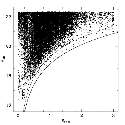
Figure 2: A plot of observed $K$-band magnitude versus photometric redshift for the galaxies in the new UDS EDR sample. The dashed line corresponds to the empirical $K-z$ relation for radio galaxies as obtained by Willott et al. (2003), which approximately coincides with the passive evolution of a $3L^{*}$ starburst formed at redshift $z_{f}=10$. The solid line corresponds to the passive evolution of a $10L^{*}$ starburst.

4 The redshift distribution of the UDS-galaxy sample

The SED fitting procedure provides two vital pieces of information for each galaxy: the best fitting galaxy template and a photometric redshift. In this Section we check the reliability of our photometric redshift estimates and compare the redshift distribution of sources in the UDS-galaxy sample with that derived by previous studies in different fields.

4.1 Spectroscopic redshifts

Figure 1 shows the comparison of our photometric redshift estimates with the spectroscopic values for $\sim 1100$ galaxies in the UDS field spanning $0<z<6$ (Yamada et al. 2005; Akiyama et al. in preparation; Smail et al. in preparation; Simpson et al. 2006a). We observe a good agreement between estimated and real redshifts in the vast majority of the cases with only $<3$% of clear outliers. The $\Delta z/(1+z)\equiv(z_{\rm spect}-z_{\rm phot})/(1+z_{\rm spect})$ has a mean of $-0.003$ with a standard deviation $\sigma=0.1$. By excluding the clear outliers (with $|\Delta z/(1+z)|>0.2$) we obtain a mean of $0.006$ with a $\sigma$ reduced to $0.04$. This accuracy is comparable to the best available from other surveys such as GOODS and COSMOS (Caputi et al. 2006; Grazian et al. 2006; Mobasher et al. 2007). The residual small focusing of the photo-z technique on the scale of $\delta z\mathrel{\hbox to0.0pt{\lower 3.0pt\hbox{$\sim$}\hss}\raise 2.0pt\hbox{$<$}}0.05$ does not affect any of our results since our binning in redshift to compute LF and colour bimodality is at least of 0.25.

The accuracy of our photometric redshift estimates is preserved also at faint K-band magnitudes. In fact, $\simeq 10$% of the sources with available spectra have magnitude $K\geq 22$ and the distribution of the $\Delta z/(1+z)$ for these sources has values for the mean and $\sigma$ consistent with the ones derived for brighter sources (see right panel of Figure 1). The statistics at those faint magnitudes is not large enough to allow us to completely exclude systematics at $z>2$ due to low signal-to-noise in the $K$-band and specially in the Spitzer IRAC bands. However, it is worth noting that for this work we focus at $z\mathrel{\hbox to0.0pt{\lower 3.0pt\hbox{$\sim$}\hss}\raise 2.0pt\hbox{$<$}}2$, a range in which our photometric redshifts are more reliable, as shown in Figure 1.

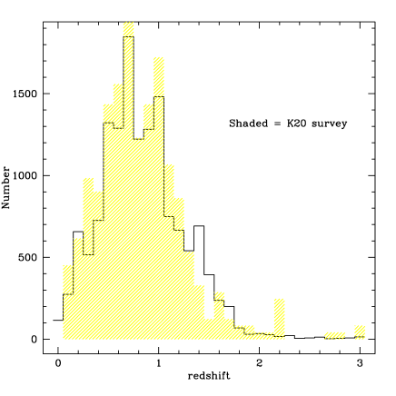
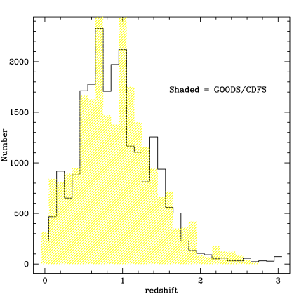
Figure 3: The estimated redshift distribution of the new UDS galaxy sample, compared with previously published redshift distributions from near-infrared samples of comparable depth but much smaller area. The solid histogram shows the distribution of photometric redshifts for sources in the UDS galaxy sample with  $K_{\rm AB}$$\leq 21.9$ and  $K_{\rm AB}$$\leq 22.5$ in the left and right panels respectively. For comparison, the redshift distributions of galaxies from the K20 survey (Cimatti et al. 2002; Mignoli et al. 2005) and GOODS/CDFS (Caputi et al. 2006; Cirasuolo et al. in preparation) are also plotted as shaded histograms in the left and right panels respectively, after normalisation to the same area as the UDS galaxy sample.

Finally, it is also worth noting the good accuracy of our photometric redshift estimates at high redshift, $z\geq 4$. In particular, in the field there is a faint galaxy which has been detected in the $K-$band ( $K_{\rm AB}$$=23.17$) with WFCAM and which has a very high spectroscopically confirmed redshift of $z=5.6$ (Ouchi et al. 2005). For this galaxy our analysis yields a photometric redshift of $z=5.5\pm 0.2$, providing additional confidence in the robustness of our redshift estimation procedure out to very high redshifts.

4.2 The K-z relation

Figure 2 shows the $K-z$ relation for the sources in the final UDS-galaxy sample. This plot illustrates the coverage of the $K-z$ plane provided by the sample, and also provides a useful sanity check that not only the overall redshift distribution, but also the photometric redshift values for individual sources are reasonable.

The dashed line represents the empirical $K-z$ relation for radio galaxies as obtained by Willott et al. (2003), which approximately coincides with the passive evolution of a $3L^{*}$ starburst formed at redshift $z_{f}=10$. The solid line corresponds to the passive evolution of a $10L^{*}$ starburst with the same formation redshift. To help minimise catastrophic errors in the photometric redshift estimation procedure, we introduced a prior which required that the redshift of the sources should not exceed the $K-z$ relation of a passively evolving $10L^{*}$ (i.e. the solid line). In fact this prior was only required for 12 galaxies, and it can be seen that the distribution of galaxies on the $K-z$ plane appears reasonable, with no significant excess of galaxies towards the bright limit.

4.3 The BzK diagram

Another consistency check on our photometric redshifts is offered by the BzK diagram. As expected, all the sources with photometric $z>1.4$ lie in the regions with $BzK\equiv(z^{\prime}-K)-(B-z^{\prime})\geq-0.2$ and $BzK<-0.2\;\cap\;(z^{\prime}-K)>2.5$ discussed by Daddi et al. (2004). In fact due to sheer number of sources in the UDS EDR sample, the BzK diagram displays a number of interesting features of relevance to galaxy evolution, some of which have not been evident in any previous studies. The BzK diagram, along with a discussion of these features, is discussed in detail by Lane et al. (2007).

4.4 Comparison with previous studies

The redshift distribution of our new UDS galaxy sample is shown in Figure 3. The left-hand panel shows (as the solid histogram) the redshift distribution for the subset of sources with  $K_{\rm AB}$$\leq 21.9$ (which corresponds to  $K_{Vega}$$\leq 20$) to facilitate comparison with the distribution obtained for the complete sample of 545 spectroscopically-confirmed sources (down to  $K_{Vega}$$=20$) in the K20 survey (Mignoli et al. 2005). The right-hand panel instead shows the redshift distribution of the UDS galaxy sample down to  $K_{\rm AB}$$\leq 22.5$ this time compared with the equivalent result obtained in the GOODS Chandra Deep Field South (CDFS) by Caputi et al. (2006) down to the same magnitude limit. Nearly half of the sources in the GOODS/CDFS have spectroscopic redshifts and the remainder have photometric redshifts computed by using 12 broad-band photometry from $\rm 0.4\mu m$ to $\rm 8\mu m$ (Cirasuolo et al. - in preparation). Both the distributions from K20 survey and GOODS/CDFS have been re-normalised to the same area as the UDS-galaxy sample.

We find a very good agreement between the redshift distribution we obtain for sources in the UDS galaxy sample and the ones displayed by the smaller samples which, however, do obviously possess a much higher fraction of spectroscopically confirmed redshifts. It is also evident from Figure 3 that the surface density of galaxies in the present sample is in agreement with those derived from these previous studies. The consistency of the redshift distributions and of the surface densities at different magnitude limits provides further confidence in the reliability of our sample and our photometric redshift estimates.

5 Luminosity Function

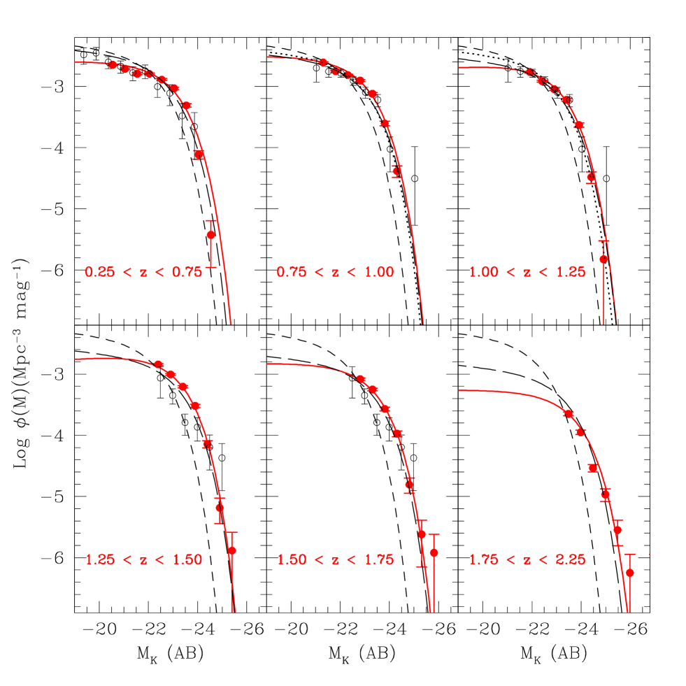
Figure 4: Rest-frame $K$-band luminosity function in six redshift bins. The solid dots show the LF obtained from the $\rm 1/V_{max}$ method for sources in the UDS sample with  $K_{\rm AB}$$\leq 22.5$. The open symbols correspond to the LF obtained from the K20 survey (Pozzetti et al. 2003) in three redshift bins ([0.2-0.65], [0.75-1.3], [1.3-1.9]), while the solid line is the best fit Schechter function obtained from the likelihood analysis. The LF obtained from the GOODS/CDFS sample (Caputi et al. 2006) is indicated by the long dashed line. Also shown, for comparison, are the LFs at $z=0$ (dashed line) and $z=1$ (dotted line) from Kochanek et al. (2001) and Drory et al. (2003), respectively.

In this Section we exploit the large area and wide redshift coverage of the UDS galaxy sample to derive the evolution of the near-infrared LF from the local Universe up to $z\mathrel{\hbox to0.0pt{\lower 3.0pt\hbox{$\sim$}\hss}\raise 2.0pt\hbox{$>$}}2$. The rest-frame $K$-band magnitudes for sources in the sample have been computed by using the closest observed band depending on the redshift of the source. This method in fact minimises the uncertainties related to the $k$-corrections, even though in the $K$-band these corrections have a small variance compared to the optical wavelengths (Cowie et al 1994; Poggianti 1997). In our case the availability of the IRAC $3.6\mu$m and $4.5\mu$m data enables us to directly trace the rest-frame $K$-band up to $z\sim 1$ for more than half of the sample. However, as a test we also compared the absolute $M_{K}$ magnitude obtained by using IRAC data with that obtained by directly extrapolating the observed $K$-band magnitude. The distribution of the difference of the magnitudes computed with these two different methods is centred around zero with rms $\sigma\sim 0.35$. Therefore, these two methods provide consistent results and for our dataset we used the $M_{K}$ estimated by using the IRAC bands when available.

Figure 4 shows the rest-frame $K$-band luminosity function (LF) in the redshift range $0.25\leq z\leq 2.25$ computed in six redshift bins by using both the classical $\rm 1/V_{max}$ method (Schmidt 1968) and the maximum likelihood analysis (Marshall et al 1983). The $\rm 1/V_{max}$ method does not require any assumption regarding the shape of the LF or parameter dependence but can be biased by strong density inhomogeneity in the field. The solid dots in Figure 4 represent the LF obtained with this method. Only the bins above the luminosity-completeness limit at each redshift bin are shown and the error bars on each point correspond to the Poissonian errors.

The solid line in Figure 4 shows the LF obtained in each redshift bin with the maximum likelihood method. This is a parametric method, for which we chose a Schechter function to describe the shape of the LF:

$$\phi(M)=0.4{\rm ln(10)}\phi^{*}10^{-0.4\Delta M(\alpha+1)}\rm exp(-10^{-0.4\Delta M})$$ (1)

with $\Delta M=M_{K}-M^{*}_{K}$. The overall normalisation ($\rm\phi^{*}$) has been obtained by matching the number of observed galaxies in each redshift bin. The best fit values for the parameters $\alpha$, $\rm M_{K}^{*}$ and $\phi^{*}$ in each redshift bin are shown in Table 1.

In the determination of the LF both in the $\rm 1/V_{max}$ method and maximum likelihood analysis a correction factor has been applied to take into account the incompleteness effects. In fact, as described in Foucaud et al. (2007), the UDS EDR sample is nearly 100% complete at  $K_{\rm AB}$$\leq 21.9$ and the completeness drops to $\sim 70$% at  $K_{\rm AB}$$=22.5$.

Due to the limiting magnitude  $K_{\rm AB}$$\leq 22.5$ our ability to trace the faint end of the LF decreases with redshift. However, up to $z\sim 1.5$ the likelihood analysis suggests that the value of the faint end slope $\alpha$ does not change with redshift and stays consistent with the local value of $\alpha\sim 1$. The actual data do not allow us any estimate of the slope for $z\mathrel{\hbox to0.0pt{\lower 3.0pt\hbox{$\sim$}\hss}\raise 2.0pt\hbox{$>$}}1.5$. Therefore, in the likelihood analysis at redshifts larger than $z=1.5$ we decided to fix the value of the faint end slope to the mean value obtained at lower redshifts ($\alpha=1$). This is consistent with the results of deeper surveys (e.g. Caputi et al. 2006). Recently, by exploiting a sample of $\sim 300$ objects selected from the Hubble deep field south (HDF-S) down to  $K_{\rm AB}$$\leq 24.9$ Saracco et al. (2006) found the value of the slope of the LF to be constant with redshift and consistent with the local value ($\alpha\sim 1$) up to $z\sim 3$.

Table 1: Best fit parameters for the Schechter LF.

z	$\alpha$	$M^{*}_{K}$	$\rm\phi^{*}(10^{-3}\;Mpc^{-3})$
$0.25-0.75$	$-0.99\pm 0.04$	$-22.86\pm 0.08$	2.9 $\pm 0.2$
$0.75-1.00$	$-1.00\pm 0.08$	$-22.86\pm 0.11$	3.4 $\pm 0.3$
$1.00-1.25$	$-0.94\pm 0.13$	$-22.93\pm 0.14$	2.8 $\pm 0.4$
$1.25-1.50$	$-0.92\pm 0.18$	$-23.03\pm 0.16$	2.6 $\pm 0.3$
$1.50-1.75$	$\rm-1.00\;fixed$	$-23.23\pm 0.09$	1.7 $\pm 0.2$
$1.75-2.25$	$\rm-1.00\;fixed$	$-23.58\pm 0.13$	0.6 $\pm 0.3$

The agreement between the estimation of the LF obtained with the two independent methods ($\rm 1/V_{max}$ and maximum likelihood) is evident in Figure 4. We also found our LF to be consistent with the results derived by Pozzetti et al. (2003) from the K20 survey and Caputi et al. (2006) from GOODS/CDFS. It is worth noting that in this work we have nearly a factor of 10 more objects compared to the GOODS/CDFS sample and a factor $\sim 40$ more than the K20 survey. Due to the large area we also have enough statistics to be able to properly trace the bright end of the LF over our full redshift range with negligible cosmic variance.

The comparison with the local LF obtained by Kochanek et al (2001) from the Two Micron All Sky Survey (2MASS) shown in Figure 4 confirms the substantial brightening of the characteristic magnitude $M^{*}_{K}$ with redshift. In agreement with previous studies (Pozzetti et al 2003; Drory et al. 2003; Feulner et al. 2003; Caputi et al. 2006; Saracco et al. 2006) we find $M^{*}_{K}$ to be brighter by $\sim 1$ magnitude at $z\sim 2$ compared to the local Universe. The lack of data at the faint end of the LF does not allow us to precisely trace the density evolution of the LF. However, up to $z\sim 1.75$ where the likelihood estimate of the best fit parameters for the LF is still reliable (see Table 1) we observe a decrease in the space density by a factor $\sim 2$ compared to $z=0$. This decrement increases up to a factor $\sim 4.5$ if the highest redshift bin is considered. This is in good agreement with the results obtained by Caputi et al. (2006) in the GOODS/CDFS as also shown in Figure 4. However, the much large statistics obtained with the current work allows for substantial improvement in determining the LF, especially at its bright end. A more detailed likelihood analysis of the LF, including the parameterisation of the evolution and the determination of the faint end slope up to the highest redshift bin will be possible with the next data release of the UDS which will reach  $K_{\rm AB}$$\sim 23.5$.

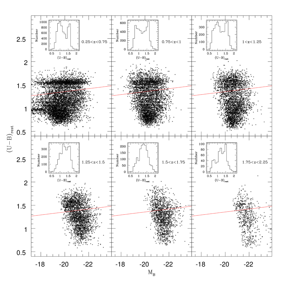
Figure 5: Rest-frame $(U-B)$ colour versus absolute magnitude in the $B$ band in six redshift intervals for sources in the UDS galaxy sample. The small insets show the distribution of the rest-frame ($U-B$) colour in each redshift bin. The diagonal line represents the luminosity-dependent colour cut (see Equation 2) adopted by van Dokkum et al. (2000) to divide the populations of red and blue galaxies.

6 The colour bimodality

Following the above analysis of the evolution with redshift of the population of $K$-band selected galaxies it is also interesting to investigate the role of the different galaxy populations and how they contribute to the global evolution of the $K$-band LF. For this purpose we analysed the rest-frame $(U-B)$ colour of sources in the UDS-galaxy sample; according to the well-studied local colour-magnitude relation (e.g. Visvanathan & Sandage 1977; Bower et al. 1992; Strateva et al. 2001) the red and blue galaxies show a bimodal distribution which allows one to easily separate the population of red/early type galaxies from the blue/late type systems.

Figure 5 shows the rest-frame ($U-B$) colour versus absolute magnitude in the $B$-band in the same six redshift intervals used for the LF. The rest-frame $U$ and $B$ band magnitudes have been computed by using the best fit template, according to the redshift of the source. The small insets in each panel show the distribution of the rest-frame $(U-B)$ colour in each redshift bin. In agreement with studies in the local Universe (Strateva et al. 2001; Hogg et al. 2002; Blanton et al. 2003a,b; Baldry et al. 2004) and at $z\sim 1$ (Bell et al. 2004a; Weiner et al. 2005; Willmer et al. 2006; Franzetti et al. 2007) we find that the colour-magnitude relation exhibits a clear bimodality up to $z\sim 1$.

The data also show the luminosity-dependent behaviour of the bimodality (Aragon-Salamanca et al. 1993; Stanford et al. 1995, 1998; Ellis et al. 1997; Kodama et al. 1998; van Dokkum et al. 2000) with the brighter sources displaying redder colours. In Figure 5 the diagonal line represents the colour-magnitude relation derived by van Dokkum et al. (2000) for red galaxies in distant clusters adding an offset of -0.25 magnitudes to separate the red and blue populations (see Willmer et al. 2006):

$$(U-B)=-0.032(M_{B}+21.52)+1.4$$ (2)

converted to the AB magnitude system. As shown in Figure 5, this luminosity-dependent colour cut is in good agreement with the observed bimodality present in the UDS galaxy sample, at least up to $z\sim 1.5$.

However, it is interesting to note that the strength of the colour bimodality fades with increasing redshift and nearly disappears at $z\mathrel{\hbox to0.0pt{\lower 3.0pt\hbox{$\sim$}\hss}\raise 2.0pt\hbox{$>$}}1.5$. The extend to which the apparent disappearance of the colour bimodality is due to photometric errors will be revealed as the UDS data progressively improve. A more detailed study on the evolution of the bimodality with redshift is beyond the scope of the present paper and will be addressed in detail by Eales et al. (2007 - in preparation).

However, it is worth noting the difficulty of the broad band rest-frame colours to distinguish between the different populations of galaxies that show the same optical and near-infrared colours, i.e. the old passive evolving sources and the dusty star-forming one. As well demonstrated in a recent paper by Stern et al. (2006) dusty starbursts and passively evolving galaxies are virtually indistinguishable in the broad band photometry at wavelengths $\leq 10\mu$m.

In the local Universe, the population of red galaxies is mostly constituted by morphologically early type objects (Sandage & Visvanathan 1978; Bower et al. 1992; Terlevich et al. 2001) and the mixing between the populations of early and late type objects is relatively low. Recent studies on the SDSS survey by Strateva et al. (2001) found only $\sim 20$% of late type galaxies to have red colours compatible with the red sequence.

This low contamination by the late type galaxies in the red sequence has also been observed at intermediate redshift ( $z<1$) both in the field (Kodama et al. 1999; Bell et al. 2004b) and in clusters (Couch et al. 1998; van Dokkum et al. 2000; van Dokkum & Franx 2001). These results are in good agreement with the well defined bimodality we observe at $z\mathrel{\hbox to0.0pt{\lower 3.0pt\hbox{$\sim$}\hss}\raise 2.0pt\hbox{$<$}}1$ in the UDS-galaxy sample (see Figure 5).

However, the contamination and the mixing between early and late type galaxies in the colour-magnitude diagram increases with redshift as clearly shown in Figure 5. Recently, Franzetti et al. (2007) exploiting data at $z\sim 1$ from the VIMOS-VLT Deep Survey (VVDS) found that even though the red peak of the colour distribution is mainly populated by early type galaxies and the blue peak by late type ones, there is a strong contamination between the two populations. In particular, they found that in the population of red galaxies only $\sim 65$% are early type galaxies, while the remaining $\sim 35$% are late type objects.

Figure 6: Rest-frame $K$-band LF for sources in the UDS-galaxy sample sub-divided by colour according to Equation 2. The solid dots represent the LF of the population of red galaxies while the open triangles show the LF of the blue objects. The dotted and long dashed lines show the LF obtained in each redshift bin by using the maximum likelihood analysis for the red and blue population respectively (see Table 2). The solid line is the LF of the whole $K$-band selected sample in each redshift bin as plotted in Figure 4 and tabulated in Table 1. For reference we also indicate by a dashed line the local $K$-band LF from Kochanek et al. (2001).

7 The Luminosity Function subdivided by colour type

As discussed in the previous Section and in Eales et al. (2007 - in prep.), classification by colour into red and blue sources provides an efficient means of identifying the population of early and late type objects at $z\mathrel{\hbox to0.0pt{\lower 3.0pt\hbox{$\sim$}\hss}\raise 2.0pt\hbox{$<$}}1$. However, as also outlined by Eales et al. the difficulties in successfully exploiting this colour selection increase with increasing redshift as demonstrated by the progressively disappearance of the colour bimodality at $z\mathrel{\hbox to0.0pt{\lower 3.0pt\hbox{$\sim$}\hss}\raise 2.0pt\hbox{$>$}}1$. Therefore, in the following Section we will study the evolution with redshift of the populations of red and blue galaxies bearing in mind that this roughly corresponds to the evolution of the early and late type objects only at low and intermediate redshift. However, it is worth remembering that even at these redshifts the cross-contamination of each population can be relatively high ($\sim 20-30$% ; Strateva et al. 2001; Ilbert et al. 2006; Franzetti et al. 2007).

Table 2: Best fit parameters for the Schechter LF of red and blue galaxies.

z	$\alpha$	$M^{*}_{K}$	$\rm\phi^{*}(10^{-3}\;Mpc^{-3})$
Blue objects
$0.25-0.75$	$-1.19\pm 0.05$	$-22.71\pm 0.11$	$1.5\pm 0.2$
$0.75-1.00$	$-1.44\pm 0.15$	$-23.05\pm 0.18$	$1.3\pm 0.2$
$1.00-1.25$	$-1.38\pm 0.19$	$-23.17\pm 0.21$	$1.3\pm 0.3$
$1.25-1.50$	$-1.43\pm 0.24$	$-23.40\pm 0.25$	$1.0\pm 0.4$
$1.50-1.75$	$\rm-1.35\;fixed$	$-23.45\pm 0.15$	$0.9\pm 0.3$
$1.75-2.25$	$\rm-1.35\;fixed$	$-23.75\pm 0.20$	$0.25\pm 0.3$
Red objects
$0.25-0.75$	$-0.12\pm 0.1$	$-22.36\pm 0.07$	$2.3\pm 0.2$
$0.75-1.00$	$-0.09\pm 0.2$	$-23.48\pm 0.13$	$2.0\pm 0.3$
$1.00-1.25$	$-0.05\pm 0.4$	$-22.65\pm 0.17$	$1.0\pm 0.3$
$1.25-1.50$	$-0.14\pm 0.5$	$-22.65\pm 0.24$	$1.0\pm 0.4$
$1.50-1.75$	$\rm-0.1\;fixed$	$-22.81\pm 0.10$	$0.7\pm 0.3$
$1.75-2.25$	$\rm-0.1\;fixed$	$-23.04\pm 0.21$	$0.2\pm 0.4$

As a first step we sub-divided the UDS galaxy sample adopting the luminosity-dependent colour cut shown by Equation 2 (van Dokkum et al. 2000). The resulting LFs for the red and blue galaxies are shown in Figure 6. As for the LF of the total sample of $K$-band selected galaxies (see Section 5) we used both the $\rm 1/V_{max}$ and maximum likelihood methods. The best fit parameters for the likelihood are shown in Table 2. Due to the limiting magnitude  $K_{\rm AB}$$\leq 22.5$ the determination of the best fit parameters in the redshift bin $1.75\leq z\leq 2.25$ is particularly challenging. Therefore, in the following discussion we consider only the redshift bins in the range $0.25\leq z\leq 1.75$ and simply comment on the behaviour in the highest z bin.

The limiting magnitude  $K_{\rm AB}$$\leq 22.5$ also does not allow us to obtain a precise determination of the faint end of the LF, as already discussed in Section 5. Therefore, the maximum likelihood analysis has been performed both leaving $\alpha$ as a free parameter as well as fixing this value to the one obtained in the lower redshift bins, where our data better trace the faint-end slope. The mean value for the parameter $\alpha$ in the redshift range $0.25\mathrel{\hbox to0.0pt{\lower 3.0pt\hbox{$\sim$}\hss}\raise 2.0pt\hbox{$<$}}z\mathrel{\hbox to0.0pt{\lower 3.0pt\hbox{$\sim$}\hss}\raise 2.0pt\hbox{$<$}}1.5$ is -1.35 and -0.1 for the blue and red objects respectively. Therefore, at $z\geq 1.5$ we fixed the slope of the LF at these values. As is clearly seen in Figure 6, the population of blue galaxies exhibits a much steeper slope compared to the red galaxies up to $z\sim 1.5$ in agreement with previous works (Lilly et al. 1995; Blanton et al. 2001; Pozzetti et al. 2003; Giallongo et al. 2005; Ilbert 2006).

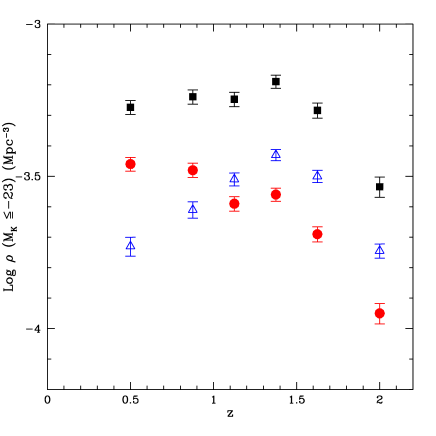
Figure 7: Space density as a function of redshift for bright sources with $M_{K}\leq-23$ classified as red (solid dots) and blue (open triangles) according to their rest-frame colours (see Equation 2). The black solid squares represent the space density of all sources with $M_{K}\leq-23$.

The redshift evolution of the blue and red populations also appears to differ. Even though both the red and blue sources experience a brightening of the characteristic magnitude $M^{*}_{K}$, the blue objects show a slightly stronger evolution with $\Delta M^{*}_{K}\sim-0.7$ over the redshift range $0.25\leq z\leq 1.75$ compared with $\Delta M^{*}_{K}\sim-0.5$ of the red population. According to the results of the maximum likelihood analysis, both populations show a small density evolution at $z\mathrel{\hbox to0.0pt{\lower 3.0pt\hbox{$\sim$}\hss}\raise 2.0pt\hbox{$<$}}1$ while at higher redshifts the decrease in number density is stronger for red objects compared with the blue ones. However, it is worth remembering that the uncertainties in the classification of the two populations based purely on the rest-frame colour cut expressed by Equation 2 can introduce severe bias, specially at higher redshift where the bimodality fades away.

The inter-connection between the luminosity and density evolution coupled with the different faint-end slope of the LFs for the two populations result in the predominance of the blue objects at faint magnitudes ($M_{K}\mathrel{\hbox to0.0pt{\lower 3.0pt\hbox{$\sim$}\hss}\raise 2.0pt\hbox{$>$}}-22$) over the whole redshift range explored in this work. On the other hand, the bright end of the LF is dominated by red objects (see Figure 6) but only up to $z\sim 1$. In fact, as shown in Figure 7 the space density of bright sources with $M_{K}\leq-23$ is nearly constant for red objects in the range $0.25\mathrel{\hbox to0.0pt{\lower 3.0pt\hbox{$\sim$}\hss}\raise 2.0pt\hbox{$<$}}z\mathrel{\hbox to0.0pt{\lower 3.0pt\hbox{$\sim$}\hss}\raise 2.0pt\hbox{$<$}}1.5$, while it increases by a factor $\sim 2$ for the blue ones over the same redshift interval. The result is that the population of the brightest objects mostly consists of red sources at low and intermediate redshift, while at $z\mathrel{\hbox to0.0pt{\lower 3.0pt\hbox{$\sim$}\hss}\raise 2.0pt\hbox{$>$}}1$ there is an inversion in the proportion with a slight predominance of blue galaxies.

It is also worth noticing that the mild density evolution of the red galaxies between $z=0$ and $z\simeq 1$ is in good agreement with the recent results by Yamada et al. (2005). These authors found that the number density of old bright passive galaxies is decreased by only a small factor (less than 2) compared with the local Universe. This is inconsistent with the results of Bell et al. (2004a) which instead suggested a decrease in the population of red galaxies by nearly a factor 10 over the same redshift range. However, as shown by Bundy et al. (2006) this decrement can be due to a selection effect. In fact, these authors pointed out how the $R$-band limit – the same band used by Bell et al. to select their sample – introduces a bias against red galaxies, especially at $z\mathrel{\hbox to0.0pt{\lower 3.0pt\hbox{$\sim$}\hss}\raise 2.0pt\hbox{$>$}}1$, and which introduces an artificially large decrease with redshift in the red population.

Figure 8: The solid dots represent the evolution of the characteristic luminosity $M_{K}^{*}$ with redshift derived from the likelihood analysis relative to the one in the local Universe ($M_{K}^{*}(z=0)=22.26$) as obtained by Kochanek et al. (2001). The dotted line is the evolution of $M_{K}^{*}$ derived by Caputi et al. (2006) from GOOD/CDFS. The solid and dashed lines represent the evolution with redshift of the $K$-band absolute magnitude derived by a single burst model from Bruzual & Charlot (2003) with formation redshifts $z=3$ and $z=6$, respectively.

8 Discussion and Conclusions

We have presented new results on the evolving near-infrared galaxy luminosity function, based on the analysis of a large sample of $K$-band selected galaxies drawn from the Early Data Release of the UKIDSS Ultra Deep Survey. The complete sample includes $\sim 22,000$ sources down to  $K_{\rm AB}$$\leq 22.5$ over an area of 0.6 square degrees. Exploiting the complementary optical and mid-IR data provided by the Subaru/XMM-Newton Deep Survey and Spitzer-SWIRE Survey we have obtained reliable photometric redshift estimates for the sources in the sample. This allowed us to study the evolution of the $K$-band LF in the redshift range $0.25\mathrel{\hbox to0.0pt{\lower 3.0pt\hbox{$\sim$}\hss}\raise 2.0pt\hbox{$<$}}z\mathrel{\hbox to0.0pt{\lower 3.0pt\hbox{$\sim$}\hss}\raise 2.0pt\hbox{$<$}}2.25$. In agreement with previous studies, we find that the characteristic luminosity of the near-infrared luminosity function exhibits a substantial brightening of $\simeq 1$ magnitude between the local Universe and $z\simeq 2$, while the total density decreases by a factor $\simeq 2$ over the same redshift interval.

We have also used the rest frame $(U-B)$ colour to separate the sample into red and blue galaxies. We find the classical bimodal colour distribution to be clearly present at $z\mathrel{\hbox to0.0pt{\lower 3.0pt\hbox{$\sim$}\hss}\raise 2.0pt\hbox{$<$}}1$. However, the strength of the colour bimodality is found to decrease with increasing redshift and virtually disappears by $z\mathrel{\hbox to0.0pt{\lower 3.0pt\hbox{$\sim$}\hss}\raise 2.0pt\hbox{$>$}}1.5$. The progressively improvement of the UDS data will assess how the errors on the photometry affect this result.

By using the colour - magnitude relation to split the sample we have analysed the cosmological evolution of the red and blue galaxy populations. The blue objects clearly dominate the faint end of the LF over the whole redshift range explored in this work. On the other hand, up to $z\simeq 1$ the brightest sources are mainly provided by red objects. In fact, the space density of red sources with $M_{K}\leq-23$ is approximately constant with redshift while the blue galaxies, with the same bright absolute magnitude, exhibit a strong increase in their space density with redshift. Therefore, this different evolutionary behaviour of the two populations determines the preponderance of blue objects in the bright-end of the luminosity function at redshifts $z\mathrel{\hbox to0.0pt{\lower 3.0pt\hbox{$\sim$}\hss}\raise 2.0pt\hbox{$>$}}1$.

Compared with previous studies, the unique combination of large area and depth of the UDS minimises the effect of the cosmic variance and has led to a substantial improvement in the determination of the LF. In particular, the large area coverage has allowed us to accurately trace the evolution of the brightest sources at $z\raisebox{-3.69899pt}{~{}\shortstack{$<$ \\ [-0.07cm] $\sim$}}~{}2$ with a high level of statistical significance. As shown in Figure 7, the space density of the total population of bright sources ($M_{K}\leq-23$) is roughly constant over the redshift range $0.5\mathrel{\hbox to0.0pt{\lower 3.0pt\hbox{$\sim$}\hss}\raise 2.0pt\hbox{$<$}}z\leq 1.5$. This strongly suggests the vast majority of the present-day bright elliptical galaxies were already in place at $z\simeq 1.5$.

On the other hand, our analysis has also shown a change in the fraction of red and blue galaxies with redshift. The majority of bright sources at $z\mathrel{\hbox to0.0pt{\lower 3.0pt\hbox{$\sim$}\hss}\raise 2.0pt\hbox{$<$}}1$ exhibit red colours consistent with having an old stellar population formed at high redshift. However, the increase of the fraction of blue galaxies with increasing redshift – indicative of an increase of the ongoing star formation – suggests the major formation epoch of the these bright sources to be at $z\mathrel{\hbox to0.0pt{\lower 3.0pt\hbox{$\sim$}\hss}\raise 2.0pt\hbox{$>$}}1.5$.

However, it is worth noting that the colour classification based on the rest-frame ($U-B$) colour is not very accurate for distinguishing between the different populations of galaxies that show the same optical colours, i.e. the old passive evolving sources and the dusty star-forming one. In fact, studies of the population of Extremely Red Objects (EROs) at redshifts $1\mathrel{\hbox to0.0pt{\lower 3.0pt\hbox{$\sim$}\hss}\raise 2.0pt\hbox{$<$}}z\mathrel{\hbox to0.0pt{\lower 3.0pt\hbox{$\sim$}\hss}\raise 2.0pt\hbox{$<$}}2$ revealed this population to be composed by both old passive evolving galaxies and dusty star-bursts, roughly in the same proportion (Cimatti et al. 2002; Smail et al. 2002; Yan & Thompson 2003; Cimatti et al. 2003; Gilbank et al., 2003; Moustakas et al. 2004; Simpson et al. 2006b).

On the other hand, not all the blue objects are experiencing their major event of star formation. In fact, it only requires less than 10% of the total mass of an early type galaxy to be involved in a recent episode of star formation to completely alter the colour of the objects and show it as a blue galaxy (Zepf 1997). This is because even a relatively small number of bright young stars dominates the emission at optical wavelengths. Moreover, a recent study from the VVDS in the redshift range $0.4\mathrel{\hbox to0.0pt{\lower 3.0pt\hbox{$\sim$}\hss}\raise 2.0pt\hbox{$<$}}z\mathrel{\hbox to0.0pt{\lower 3.0pt\hbox{$\sim$}\hss}\raise 2.0pt\hbox{$<$}}0.8$ by Ilbert et al (2006) found that $\sim 30$% of bulge dominated sources exhibit blue colours, indistinguishable from the late type population (see also Im et al. 2001; Menanteau et al. 2004; Cross et al. 2004).

It is also interesting to notice that the brightening of the characteristic luminosity ($M_{K}^{*}$) of the whole $K$-band selected LF is consistent with the passive evolution of a single stellar population. Figure 8 shows the evolution of $M_{K}^{*}$ derived from our likelihood analysis relative to $M_{K}^{*}$ at z=0 (Kochanek et al. 2001). Within the errors, our data agree remarkably well with the evolution of the $K$-band absolute magnitude displayed by a single burst model from Bruzual & Charlot (2003) with formation redshifts in the range $3\mathrel{\hbox to0.0pt{\lower 3.0pt\hbox{$\sim$}\hss}\raise 2.0pt\hbox{$<$}}z\mathrel{\hbox to0.0pt{\lower 3.0pt\hbox{$\sim$}\hss}\raise 2.0pt\hbox{$<$}}6$. This result, coupled with the constant space density of bright sources up to $z\simeq 1.5$, suggests the major assembly epoch of bright sources to be at $z\mathrel{\hbox to0.0pt{\lower 3.0pt\hbox{$\sim$}\hss}\raise 2.0pt\hbox{$>$}}2$, even though spread over a large range in redshift. In fact, as shown from Figure 7, nearly 40% of the bright sources at $z\simeq 1.5$ exhibit red colours. Assuming that half of them are dusty starbursts – as suggested by studies of ERO populations (e.g. Cimatti et al. 2002) – we end up inferring that at least 20% of sources are old passively evolving galaxies at these redshift. Therefore, this implies that a reasonable fraction of bright sources at $z\simeq 1.5$ was assembled at very high redshift with very efficient star formation.

9 acknowledgements

MC, SF and CS would like to acknowledge funding from PPARC. RJM, OA and IS would like to acknowledge the funding of the Royal Society. We are grateful to the staff at UKIRT and Subaru for making these observations possible. We also acknowledge the Cambridge Astronomical Survey Unit and the Wide Field Astronomy Unit in Edinburgh for processing the UKIDSS data.

References

- [1] Aragon-Salamanca, A., Ellis R.S., Couch W.J., Carter D., 1993, MNRAS, 262, 764
- [2] Baldry, I. K., Glazebrook, K., Brinkmann, J., Ivezić, Ž., Lupton, R. H., Nichol, R. C., Szalay, A. S., 2004, ApJ, 600, 681
- [3] Bell, E. F., et al., 2004a, ApJ, 608, 752
- [4] Bell, E. F., et al., 2004b, ApJ, 600, L11
- [5] Bertin, E., & Arnouts, S., 1996, A&A Supplement, 117, 393
- [6] Blanton, M. R., et al., 2001, AJ, 121, 2358
- [7] Blanton, M. R., et al., 2003a, ApJ, 594, 186
- [8] Blanton, M. R., et al., 2003b, ApJ, 592, 819
- [9] Bolzonella M., Miralles J.-M., & Pelló, R., 2000, A&A, 363, 476
- [10] Bower, R. G., Lucey, J. R., Ellis, R. S., 1992, MNRAS, 254, 601
- [11] Brotherton, M. S., Tran, H. D., Becker, R. H., Gregg, M. D., Laurent-Muehleisen, S. A., White, R. L. 2001, ApJ, 546, 775
- [12] Bruzual G., Charlot S., 2003, MNRAS, 344, 1000
- [13] Bundy K., et al., 2006, ApJ, 651, 120
- [14] Calzetti D., Armus L., Bohlin R.C., Kinney A.L., Koornneef J., Storchi-Bergmann T., 2000, ApJ, 533, 682
- [15] Caputi, K. I., McLure, R. J., Dunlop, J. S., Cirasuolo, M., Schael, A. M. 2006, MNRAS, 366, 609
- [16] Cimatti A., et al. 2002, A&A, 381, L68
- [17] Cimatti, A., et al., 2003, A&A, 412, L1
- [18] Cole, S., et al., 2001, MNRAS, 326, 255
- [19] Coleman, G. D., Wu, C.-C., Weedman, D. W., 1980, ApJS, 43, 393
- [20] Coppin K., et al., 2006, MNRAS, 372, 1621
- [21] Couch, W. J., Barger, A. J., Smail, I., Ellis, R. S., Sharples, R. M., 1998, ApJ, 497, 188
- [22] Cowie, L. L., Gardner, J. P., Hu, E. M., Songaila, A., Hodapp, K.-W., Wainscoat, R. J., 1994, ApJ, 434, 114
- [23] Cowie, L. L., Songaila, A., Hu, E. M., Cohen, J. G., 1996, AJ, 112, 839
- [24] Cross, N. J. G., et al., 2004, AJ, 128, 1990
- [25] Daddi E., Cimatti A., Renzini A, Fontana,A, Mignoli M., Pozzetti L., Tozzi P., Zamorani G., 2004, ApJ, 617, 746
- [26] Dickinson, M., Papovich, C., Ferguson, H. C., & Budavári, T., 2003, ApJ, 587, 25
- [27] Drory, N., Bender, R., Feulner, G., Hopp, U., Maraston, C., Snigula, J., Hill, G. J., 2003, ApJ, 595, 698
- [28] Drory N., Salvato M., Gabasch A., Bender R., Hopp U., Feulner, G., Pannella, M., 2005, ApJL, 619, L131
- [29] Dunlop, J.S., Guiderdoni, B., Rocca-Volmerange, B., Peacock, J.A., Longair, M.S., 1989, MNRAS, 240, 257
- [30] Dye S., et al., 2006, MNRAS, 372, 1227
- [31] Ellis, R. S., Smail, I., Dressler, A., Couch, W. J., Oemler, A. J., Butcher, H., Sharples, R. M., 1997, ApJ, 483, 582
- [32] Feulner, G., Bender, R., Drory, N., Hopp, U., Snigula, J., Hill, G. J., 2003, MNRAS, 342, 605
- [33] Fontana A., et al., 2004, A&A, 424, 23
- [34] Foucaud S., et al., 2007, MNRAS, 376, L20
- [35] Franzetti P., et al., 2007, A&A, 465, 711
- [36] Gabasch, A., et al., 2004, A&A, 421, 41
- [37] Giallongo, E., Salimbeni, S., Menci, N., Zamorani, G., Fontana, A., Dickinson, M., Cristiani, S., Pozzetti, L., 2005, ApJ, 622, 116
- [38] Gilbank, D. G., Smail, I., Ivison, R. J., Packham, C., 2003, MNRAS, 346, 1125
- [39] Glazebrook, K., Peacock, J. A., Miller, L., & Collins, C. A., 1995, MNRAS, 275, 169
- [40] Glazebrook, K., et al., 2004, Nature, 430, 181
- [41] Glikman E., Helfand, D. J., White, R. L., 2006, ApJ, 640, 579
- [42] Grazian A., et al., 2006, A&A, 449, 951
- [43] Hewett P. C., Warren S. J., Leggett S. K., Hodgkin, S. T., 2006, MNRAS, 367, 454
- [44] Hogg, D. W., et al., 2002, AJ, 124, 646
- [45] Ilbert, O., et al.l, 2006, A&A, 453, 809
- [46] Im, M., Faber, S. M., Gebhardt, K., Koo, D. C., Phillips, A. C., Schiavon, R. P., Simard, L., Willmer, C. N. A., 2001, AJ, 122, 750
- [47] Kinney, A. L., Calzetti, D., Bohlin, R. C., McQuade, K., Storchi-Bergmann, T., Schmitt, H. R., 1996, ApJ, 467, 38
- [48] Kodama, T., Arimoto, N., Barger, A. J., Arag’on-Salamanca, A., 1998, A&A, 334, 99
- [49] Kodama, T., Bower, R. G., Bell, E. F., 1999, MNRAS, 306, 561
- [50] Kochanek, C. S., et al., 2001, ApJ, 560, 566
- [51] Lawrence, A., et al., 2006, MNRAS, submitted, astro-ph/0604426
- [52] Lane K. P., et al., 2007, MNRAS accepted, astro-ph/0704.2136
- [53] Lilly, S. J., Longair, M.S., 1984, MNRAS, 211, 833
- [54] Lilly, S. J., Tresse, L., Hammer, F., Crampton, D., Le Fevre, O., 1995, ApJ, 455, 108
- [55] Lonsdale C.J., et al. 2003, PASP, 115, 897
- [56] Lonsdale C.J., et al. 2004, ApJS, 154, 54
- [57] Madau P., 1995, ApJ, 441, 18
- [58] Maddox N., & Hewett, P. C., 2006, MNRAS, 367, 717
- [59] Marshall, H. L., Tananbaum, H., Avni, Y., Zamorani, G., 1983, ApJ, 269, 35
- [60] Menanteau, F., et al., 2004, ApJ, 612, 202
- [61] Mignoli, M., et al., 2005, A&A, 437, 883
- [62] Miyazaki S., et al., 2002, PASJ, 54, 833
- [63] Mobasher B., et al., 2007, ApJS, astro-ph/0612344
- [64] Mortier A.M.J., 2005, MNRAS, 363, 563
- [65] Moustakas, L. A., et al., 2004, ApJL, 600, L131
- [66] Oke, J. B., & Gunn, J. E., 1983, ApJ, 266, 713
- [67] Ouchi, M., et al., 2005, ApJ, 620, L1
- [68] Poggianti, B. M., 1997, A&AS, 122, 399
- [69] Poli, F., et al., 2003, ApJL, 593, L1
- [70] Pozzetti, L., et al., 2003, A&A, 402, 837
- [71] Sandage, A., & Visvanathan, N., 1978, ApJ, 225, 742
- [72] Saracco, P., et al., 2006, MNRAS, 367, 349
- [73] Schmidt, M., 1968, ApJ, 151, 393
- [74] Sekiguki K., et al., 2005, in Renzini A. & Bender R., ed., Multiwavelength mapping of galaxy formation and evolution. Springer-Verlag, Berlin, p82
- [75] Simpson C., et al.,2006a, MNRAS, 372, 741
- [76] Simpson C., et al., 2006b, MNRAS 373, L21
- [77] Smail, I., Owen, F. N., Morrison, G. E., Keel, W. C., Ivison, R. J., Ledlow, M. J., 2002, ApJ, 581, 844
- [78] Stanford S.A., Eisenhardt P.R.M., Dickinson M., 1995, ApJ, 450, 512
- [79] Stanford S.A., et al., 1998, ApJ, 492, 461
- [80] Stern D., Chary R.-R., Eisenhardt P. R. M. Moustakas L. A., 2006, AJ, 132, 1405
- [81] Strateva, I., et al., 2001, AJ, 122, 1861
- [82] Surace J., et al. 2005, Technical report, The SWIRE Data release 2, http://swire.ipac.caltech.edu/swire/astronomers.html
- [83] Terlevich, A. I., Caldwell, N., Bower, R. G., 2001, MNRAS, 326, 1547
- [84] van Dokkum, P. G., Franx, M., Fabricant, D., Illingworth, G. D., Kelson, D. D., 2000, ApJ, 541, 95
- [85] van Dokkum, P. G., & Franx, M., 2001, ApJ, 553, 90
- [86] Visvanathan, N., & Sandage, A., 1977, ApJ, 216, 214
- [87] Willmer C.N.A., et al., 2006, ApJ, 647, 853
- [88] Weiner, B. J., et al., 2005, ApJ, 620, 595
- [89] Willott, C. J., Rawlings, S., Jarvis, M. J., Blundell, K. M., 2003, MNRAS, 339, 173
- [90] Yan, L., & Thompson, D., 2003, ApJ, 586, 765
- [91] Yamada, T., et al., 2005, ApJ, 634, 861
- [92] Zepf, S. E., 1997, Nature, 390, 377