Abstract

We report high-spectral resolution observations of comet 9P/Tempel 1 before, during and after the impact on 4 July 2005 UT of the Deep Impact spacecraft with the comet. These observations were obtained with the HIRES instrument on Keck 1. We observed brightening of both the dust and gas, but at different rates. We report the behavior of OH, NH, CN, C₃, CH, NH₂ and C₂ gas. From our observations, we determined a CN outflow velocity of at least 0.51 km sec^-1. The dust color did not change substantially. To date, we see no new species in our spectra, nor do we see any evidence of prompt emission. From our observations, the interior material released by the impact looks the same as the material released from the surface by ambient cometary activity. However, further processing of the data may uncover subtle difference in the material that is released as well as the time evolution of this material.

Proposed Running Head: Keck Observations of Tempel 1

1 Introduction

On 4 July 2005 UT, the Deep Impact spacecraft impacted comet 9P/Tempel 1. The goal of the impact experiment was to expose deep layers of the comet nucleus to study the chemical composition of those layers and to ascertain the structural properties of the nucleus.

Comets are the remnant building blocks from the outer solar nebula. The majority of their lifetimes are spent at large heliocentric distances so they undergo little chemical evolution. However, even far from the Sun, the outer layers are altered via radiation darkening (Strazzula and Johnson 1991). Once comets enter the inner Solar System, sublimation removes outer layers, while mantling covers the exterior with dust.

Comet 9P/Tempel 1 is a Jupiter family comet which has made many passages into the inner Solar System and has not been extremely far from the Sun in many orbits. Thus, the expectation was that there was an altered outer layer to the comet, but that the interior was pristine. The outer layer is thought to be too deep for a small drill carried by a spacecraft to penetrate to pristine material. In order to reach fresh, unaltered material, the Deep Impact mission proposed to create a large crater by placing a small (370kg) spacecraft in the path of the comet, setting up an impact. The impact occurred on 4 July 2005 at 05:44:36 UT (Earth-received time of 05:52:02 UT). The impact speed was 10.3 km/sec resulting in an impact kinetic energy of 19 GJ (A’Hearn et al. 2005).

The impactor was carried by a larger flyby spacecraft which was able to monitor the impact with high spatial resolution. However, while the flyby spacecraft carried an IR spectrometer, it was not able to perform optical spectroscopic observations of the impact, nor was it able to monitor the comet for many days after impact. Thus, a ground-based campaign was established in order to monitor changes in the comet (Meech et al. 2005).

We observed the impact and its aftermath from the Keck 1 telescope using the HIRES spectrograph as part of the ground-based campaign. High resolution spectra could be used to monitor aspects of the impact which could not be observed at lower spectral resolution. These include monitoring isotope ratios to determine whether the ices in the interior of the comet are isotopically similar to the ices we normally see subliming from the surface. Jehin et al. (2006) reported the isotopic ratios for ¹²C/¹³C and ¹⁴N/¹⁵N, both during the first few hours after impact and at times other than the impact. They showed that the excavated material is isotopically similar to the normal outgassing. High resolution spectra allow for detailed examination of the rotational states of the molecules. This allowed us to determine whether any prompt emissions were seen or whether the impact produced any rotationally hot lines. High resolution also allowed for detection of any new, unexpected species. High resolution data are more sensitive to very weak lines than low resolution spectra because higher spectral resolving power disperses the underlying continuum to a greater extent, resulting in higher line-to-continuum contrast (our spectral resolution of $\sim$6 km sec^-1 was not sufficient to resolve typical cometary lines with widths of $\sim$1 km sec^-1).

2 Observations and Reductions

The data were obtained with the Keck 1 telescope and HIRES spectrograph (Vogt 1992) on 30 May 2005 and 4–6 July 2005 UT (see table 1 for details of the observations). The Keck HIRES operates with three $2048\times 4096$ Lincoln Lab CCD detectors with 15 $\mu$m pixels. Typically, the detectors are binned in the spatial direction, resulting in 1024 spatial pixels of 0.24 arcsec projected on the sky. The spectrograph has two cross dispersing gratings to preferentially image the blue or the red part of the spectrum. We used the UV cross disperser (despite the wavelength covered, the convention is to call the chips blue, green and red and we will use these names throughout this paper; blue covers 3047–3951Å, green covers 3971–4926Å, and red covers 4977–5894Å). The slit was the “C1” slit, which images $7\times 0.86$ arcsec of the sky (or $4570\times 562$ km at the comet’s distance). This results in a nominal resolving power, $\lambda/\Delta\lambda=47,000$ with the slit projecting to 4.8 pixels on the detector. The slit was set at the parallactic angle, which means that it rotated on the sky during the night. The slit orientation is listed in table 1. By setting the slit at the parallactic angle, we ensured that atmospheric dispersion changed the position of the comet along the slit, minimizing loss of light on the slit. However, it did mean that we sampled slightly different coma regions throughout the night. Thus, we could be sampling overdense regions differently at different times.

On all nights, bias frames, flat field and ThAr lamps were observed for calibration (darks were not obtained because these chips typically have almost no dark current; however, as we will discuss below, this turned out not to be the case in July). During the July observations we also observed a solar analogue star (HD159222 on 4 July (Hardorp 1978) and 18 Sco (Porto de Mello 1997) on 5 and 6 July) to be able to remove the dust continuum and a rapidly rotating hot star (HR 7279 on 4 July and HR 7415 on 5 and 6 July) to be able to remove telluric features. On 30 May and 4 July a flux standard was observed.

On 30 May 2005, three 20-minute spectra were obtained as part of the Keck Director’s time. These observations were intended to give a pre-impact baseline of how the spectrum of the coma looked in its normal state.

The observations of 4 July 2005 started during nautical twilight, at 05:36:15, so that we could obtain a pre-impact spectrum. Eight degree twilight was at 05:29UT; 12 degree twilight (nautical) was at 05:58UT; 18 degree twilight (astronomical) was at 06:28. Since it was not fully dark, the signal from the sky was substantial in this first spectrum. The second spectrum was started at approximately the impact time (start at 05:55:18 UT, about 3 minutes after impact). We were guiding directly on the comet so we could watch the coma brightening. The exposure time chosen was a compromise between obtaining sufficient signal/noise and keeping as rapid a cadence as possible. The observations continued until 09:41:10 UT. The exposure times were lengthened as the comet dimmed again after the impact and the airmass of the comet increased.

We observed the comet to brighten rapidly within a few minutes of impact and to gradually fade as we continued to observe. This is in accord with other observers (Meech et al. 2005; Schleicher et al. 2006). We will discuss the trends of what we observed more in the next section.

The observations of 4 July 2005 were obtained as Keck Director’s time. The observations of 30 May and 4 July are available to the public from the Keck archive. Because of the data reduction issues discussed below, we suggest that people interested in obtaining data from the archive download raw and not processed data.

We also obtained observations on 5 and 6 July 2005 UT to follow up on the behavior of the comet after the impact. For some of the spectra on these two nights, we offset the telescope from the optocenter to be able to probe the distribution of the gas in the coma. The offset positions are noted in the log. The night of 6 July had some clouds, whereas 30 May and 4 and 5 July were photometric. Because of the clouds on 6 July, these observations were used only for the isotopic abundances but not for monitoring the cometary activity.

Keck Observatory has a data reduction pipeline, MAKEE, which many observers use. However, since it assumes that the target is a point source and the ends of the slit are sky, it is not appropriate for the reduction of cometary data. Note that the reduced versions of the data in the archive have been reduced with the MAKEE pipeline so should be used with caution.

We reduced all four nights’ data with the echelle package in IRAF. Each chip was split out to a separate file and the chips were processed in parallel. Zero and bias correction and trimming were first performed. The first 7 pixels and pixels greater than 4000 in the spectral direction are no good for any chip. All the images were then flat fielded.

While building flat field images for the July data, we discovered an enhanced background in the spectral images. This manifests itself as a signal that is measurable in the inter-order gaps. At first, we assumed that this was scattered light in the spectrograph. However, inspection of the comet frames showed that this background scaled with exposure time, as if there was a high dark current. This effect was absent in the May data. We cannot confirm whether the darks were indeed elevated for our observations since the dewar had been opened for unrelated reasons before we realized the extent of the background problem.

Regardless of the reason for the background, we needed to remove this from all the spectra or it would have added an unwanted offset to all spectra. For the green and red chip this was not difficult. It could be removed with the apscatter routine for the flat fields. For the cometary spectra, we fit a surface to the inter-order region, working in small sections around each order.

Handling the blue chip background was more complicated because the blue-most orders overlap one another slightly. We could define the trace of the spectrum on the chip with a slit which was less tall than the 7 arcsec slit we were using for targets. However, with no inter-order gap between some orders in the actual comet spectra, there was no background to fit a surface. Therefore, we built a “background” image from a flat obtained with the shorter slit, scaled that image to the background of the individual cometary spectra and subtracted it from the comet spectra. The fact that the background fit to a flat field spectrum was the same shape as that underneath the cometary spectra argues again for a dark current-like source, rather than scattered light since the comet and the flat field are different colors.

Once the data were flat fielded, the spectra for each order were extracted. We used variance weighting to collapse the spectrum spatially. We defined the extent of the slit on the chip with the flat field images. We fit the dispersion curve to the ThAr lamp spectra. The typical rms for the wavelength solution for each chip was 0.004Å. The cometary spectra were Doppler shifted to the spectrograph rest frame using the orbital information.

In order to determine the behavior of the dust and coma gas as a function of time, we first corrected the spectra for extinction using mean extinction coefficients for Mauna Kea Observatory (as given on the Keck Telescope web site; Hodapp (personal communication) reported that the extinction was normal for Mauna Kea on 4 July and inspection of our solar analogue spectra confirm this). This results in spectra as if seen outside the atmosphere. Then, since we obtained the spectra with a variety of exposure times, each spectrum was normalized to the equivalent count rate for a 15 minute exposure (our most common exposure time on 4 July).

Cometary spectra consist of three component parts: the emission spectrum of the gaseous coma, mostly as the result of resonance fluorescence; the continuous spectrum which underlies the emission that results from the solar light being reflected from the dust; the telluric spectrum being superposed on the comet spectrum. The telluric spectrum only shows up in some orders.

In order to study the gaseous component, we used the spectra of the solar analogue stars as a proxy for the solar spectrum and shifted these spectra to align the absorption features with the cometary absorption features. The stellar spectra were scaled to match the continuum of the comet spectra and then subtracted. The process was done interactively, with the aim of having no features left in the continuum regions. This shift and scale process was performed on each order independently.

There were several problems which we encountered with this process. For some of the orders, especially the bluest orders and observations at high airmass, the continuum in the comet spectra was very weak, so it was difficult to align the stellar and cometary spectra. In those cases we relied on shifts derived at lower airmass or redder wavelengths, assuming that all spectra in a given spectral image and night had the same shift. This assumption is accurate to the nearest pixel but not to sub-pixel values of the shifts. However, since in these cases the solar continuum contributed little to the cometary spectra, incorrect shifts at this level introduce very little additional noise.

For the first spectrum on 4 July, which was obtained with a bright sky, we actually had two continuum spectra imposed on each gas spectrum. The first was the cometary. The second was the Earth’s blue sky. The sky spectrum dominated the signal and was not at the same Doppler shift as the cometary spectrum. Thus, when removing the continuum, we preferentially removed the sky spectrum but would end up with a noisy comet spectrum from the slight wavelength offset between the comet and sky spectra.

The most important problem which we encountered for interpretation of what happened during the aftermath of the impact was that the continuum brightened much more and faster than did the gas. For most orders, this was just taken into account by the scaling process. However, we had problems removing the continuum for the spectral order which contains the CN $\Delta v=0$ band. In that order, in the first few spectra where the continuum was strongest, we found that if we used the criterion that there should be no absorptions left between the P and R branches, it would appear that we had over-subtracted continuum to the blue and red of the band and had imposed “emission” features. If we ended up with a smooth continuum to the blue and (especially) red, then we ended up with absorptions left between the R and P branches. We compromised and ended up with some absorption between the branches. This effect is illustrated in Fig. 1 and most affected spectra 67–70.

In general, the continuum was strongest in spectra 67–70 and these spectra had relatively short exposure times. Thus, these are the spectra for which the spectral regions between the lines are noisiest and therefore, these are the spectra with the lowest signal/noise.

Once the continuum has been removed, the resultant spectra represent the pure gaseous emission from the comet. We can subtract these gas spectra from the original spectra, yielding pure continuum spectra. These continuum spectra give a measure of the dust.

3 Results

3.1 Dust

Once we have separate dust and gas spectra we can investigate the trend of each with time after the impact. Since there are no distinct dust features, we maximized the signal/noise by averaging the dust spectra by chip. In practice, to avoid edge effects, we averaged the middle 2000 pixels in wavelength and all except the first and last order on each chip. For each spectral image, this results in three average values centered at $\sim 3460$, $\sim 4475$, and $\sim 5425$Å (the “bandpasses” are approximately 750Å wide). The upper panel of Fig. 2 shows the trend of the dust in the three chips as a function of time. Note that the average counts peaked approximately 2300 sec after the impact and then declined. The peak is less distinct in the blue chip data than the green and red chips. This may or may not be significant since the signal is so much lower at these blue wavelengths. The error bars on these data are based on Poisson statistics of the average counts. However, since each average is computed from 18,000 – 38,000 pixels, these error bars are extremely conservative.

The initial rise in the average counts indicates that the impact released a large amount of material, increasing the scattering cross-section. This brightening can come from both an increase in the number of particles, as well as from a change in particle size distribution to a larger fraction of smaller particles. A change in particle size distribution could potentially result in a change in dust color, depending on the particle sizes relative to the wavelength of observation.

We can look at the color evolution of the dust by ratioing the average counts of the different chips. These colors are shown in the lower panel of Fig. 2. We see no change in the color of the dust during our observations of 4 July (note that the 4 July observations span a large range of airmass so the lack of a color change corroborates the reasonableness of the adopted extinction coefficients). We also show the average values for 30 May and 5 July for both the individual chip counts and for the colors (averaging only those observations when the slit was centered on the optocenter). The colors are similar on all three nights, though the 4 July data may be slightly redder. However, within the error bars, the dust is the same color on 4 July as on 30 May or 5 July. This would be in contrast with the Spitzer observations, where they report a “bluening” of the scattered light (Lisse et al. 2006), and with Schleicher et al. (2006), who noted that the material was redder in color than the general inner coma in the first 15 minutes.

The average counts for each chip show that the continuum count rate was lower on 5 July than when we stopped obtaining spectra on 4 July. The 5 July count rate was similar to the 30 May count rate so probably represents the ambient level.

If the particles are around 0.5–1$\mu$m in size, as observed by Sugita et al. (2005), or even in the 0.5–2.5$\mu$m size range as observed by Schleicher et al. (2005), we would have seen a change in color if the particles changed size substantially. Since we do not see a change in color, there was not substantial fragmentation or sublimation of the dust in these first two days.

3.2 Gas

The observations spanned a large wavelength range so we were able to observe many molecular emission features. These included OH, NH, CN, C₃, CH, C₂ and NH₂. All of these species are radicals and are believed to be either daughter or granddaughter species. The emission spectra are formed via resonance fluorescence. When the impact occurred, some volatile and non-volatile material was thrown out of the crater. Keller et al. (2005) argue that the impact energy was insufficient, by a factor of several hundred (Küppers et al. 2005) to sublimate the observed amount of water molecules, so there was unlikely to be vapor released because of the impact. Then, the ices needed to sublime to form the parent gases and finally they dissociated to form the daughter and granddaughter species. Each dissociation step has a characteristic lifetime, which is typically longer than the time for the material to flow out of our, rather small ($0.86\times 7$ arcsec or 562$\times$4570 km), aperture. However, some of any parent will be dissociated instantly, while other molecules of that parent will take more time, so that the lifetime is an e-folding time for the dissociation process to take place. The signal which we observe is that which is imposed upon the ambient spectrum of the cometary coma had there been no impact.

We can achieve the highest signal/noise for extracted spectra by summing the whole length of the 7 arcsec slit. However, we then must try to deconvolve the effects of outflow from the effects of the impact. In order to understand better the impact effects, we extracted the spectra only over the spatial resolution of the telescope – the inner 0.7 arcsec (457 km) or 3 pixels in the spatial direction (the slit width of 0.86 arcsec or 562 km still defines the spectral resolution of the observations). These spectra from the inner pixels still incorporate some of the coma at large distances along the line of sight but the relative contribution of the near nucleus region to the coma is increased over spectra extracted along the full length of the slit. As would be expected, these spectra are considerably fainter than whole slit spectra (a 10 meter telescope does have its limitations!) and have lower signal/noise. In addition, we are prone to the effects of noise spikes (radiation events) in the extracted spectra since the cleaning algorithm for such spikes is not effective when only sampling 3 pixels. We had to edit out noise spikes by hand and some of the smaller spikes remain (unfortunately not all the noise spikes are single pixels since radiation events can strike the chip obliquely). Fig. 3 shows pieces of the spectra for each of the species listed above. In this figure, we show the first spectrum after the impact (file 66), another spectrum towards the end of 4 July (file 75) and a spectrum at the start of 5 July (file 129).

From inspection of Fig. 3 some trends emerge. First, the comet was not very gaseous to begin with. If we difference the last pre-impact spectrum (number 65) from the first post-impact spectrum (number 66), we find there are no additional emissions seen over the ambient cometary spectrum. Thus, in the first 10 minutes, no increased emission was detected and the left-hand panel of Fig. 3 for each molecule shows, in essence, the ambient cometary spectrum.

All of the species show an increase in line strength in response to the impact. However, the relaxation timescale back to the ambient spectrum was different for different species. The CN increases dramatically in strength from the impact to the spectrum 2 hours later, but by 5 July it is back to its pre-impact level. Note, however, that the rotational structure of the emissions does not change due to the impact. This is true for all species and argues that there is no prompt emission component due to the impact and that all species continue to be excited only by resonance fluorescence.

The OH spectra shown here are extremely noisy. This is especially true of the spectrum at 08:16 on 4 July because of the large airmass. While we corrected for the extinction, these emissions would be the ones most affected by any errors in the extinction coefficients applied. Also, if the extinction is severe enough that most photons are blocked before they reach the detector, no correction will repair the signal. We will discuss OH more when we discuss full slit extractions below.

C₃ shows an increase in brightness on 5 July from the first spectrum on 4 July but this perceived increase may be due to the noise in spectrum 66 (recall that this spectrum was obtained in the first 10 minutes after the impact).

Inspection of Fig. 3 shows that the C₂ was essentially unchanged (except for the noise level) from the end of 4 July to the beginning of 5 July (note that the strong line at around 5155Å is an NH₂ line, not C₂). More can be said about the C₂ if we can increase the signal/noise by summing along the whole slit. This is discussed below.

NH is the only molecule which is essentially as bright on 5 July as it was near the end of 4 July. The NH₂, however, shows a decay back to the ambient level by 5 July. If, as we believe, NH₃ is the parent of NH₂ and the grand-parent of NH, the earlier decay of the NH₂ would be expected.

CH does not appear to be present in either the first or last spectra. It is, however, present in the spectrum at 08:16 on 4 July. This molecule’s spectrum is helped tremendously by extraction along the complete length of the slit.

In order to boost the signal/noise, we next re-extracted the spectra, collapsing the spectra from the full length of the slit. These spectra are shown in Fig. 4. Spectra are shown at the same three times as in Fig. 3.

In these full-slit extracted spectra, we see the same trend for CN as we did in the inner three pixels. Recall that spectrum 66, the first shown here, is essentially an ambient cometary spectrum.

The OH appears to continue to increase in line strength for the 5 July spectrum. This must be viewed with caution because OH is the molecule which is most affected by the increasing airmass of the observations on 4 July. The observation at 08:08 UT was while the comet was at $\sim 1.8$ airmasses and the extinction is around 1.4 magnitudes/airmass at this wavelength, even at the high elevation of Mauna Kea. Small errors in the extinction coefficient used would have a large effect. However, it is apparent that the OH did not decrease much, if at all, by 5 July.

Inspection of Fig. 4 shows that C₂ was essentially unchanged from the end of 4 July to the beginning of 5 July, but is stronger than the ambient spectrum. Recall that C₂ has no dipole moment and thus has no easy relaxation pathway. This is also why we normally see such high J-levels for C₂. All of the apparent “noise” to the blue of the bandhead is C₂ lines which are so weak in the first spectrum that they are not easily discerned.

The behavior of C₃ is intermediate to that of the CN and C₂. It is clearly still stronger on 5 July than the first spectrum, but it is only half as strong as it was at 08:08 UT.

The NH₂ is just as strong on 5 July as it was at the end of 4 July when integrated along the whole slit, while the NH has decreased in strength. With the very blue wavelength of the NH emissions, it would be affected more by extinction than would the NH₂, which would argue that it might be even slightly brighter for the late spectrum on 4 July. Recall that when we examined the spectra of these two species in just the inner three pixels spatially, the NH₂ actually dimmed sooner than NH, as would be expected if NH₃ is the dominant parent of NH. Thus, the reversed trend we see here must be a function of the dissociation of the species.

CH behaved like the CN, having almost returned to its pre-impact value by the next night. It seems to be only slightly stronger at the start of 5 July than the first observation on 4 July.

In order to follow the trend of the various species with time in more detail, we integrated select emission lines for each molecule. In general, we fit a continuum under the emission lines and added up the flux above the continuum in each line individually and summed a series of lines. For C₂, it is impossible to use individual lines so we summed the bandhead. For C₃, we used the Q- and part of the R-branch. The integrated intensities are shown in Fig. 5. It is again obvious that not all species behaved alike. As with Fig. 4, the values shown here are for the spectra integrated along the full length of the slit. All of the species are normalized to the value for that species in spectrum 66, the first post-impact spectrum. However, remember that we saw no emission increase in this spectrum so the value of 1 in this plot represents the ambient cometary emission.

We measured 9 R-branch lines and 10 P-branch lines of CN [the “lines” are actually unresolved blends of two closely spaced lines e.g. R₁(11) + R₂(10)]. After the impact, the CN lines grew stronger for the first 4500 seconds and then the intensity of the lines began to decrease. At their maximum, the integrated line intensity was 3 times greater than at the time of impact. Recall that the slit was $0.86\times 7$ arcsec, which corresponds to $562\times 4570$ km at the comet’s distance. If all of the CN is produced instantaneously and no more is produced after the impact, then 4500 sec represents the time for the material to start flowing out of the aperture. Since the impact was a distinct impulse which caused a release of material from the impact site, what we measured was the increasing cross section as the material expanded away from the nucleus. Eventually, the area which was fluorescing grew larger than the footprint of our slit on the cometary coma and we were no longer able to measure all of the material, though our aperture does still include the material coming directly towards us. That point came at approximately 4500 sec after the impact, causing the diminution of light we observe. If the CN was only produced instantaneously, then the diminution at 4500 sec indicates that the material was flowing outwards at 0.51 km sec^-1. This is twice as large as the outflow velocity of 0.2 km sec^-1 and of 0.23 km sec^-1 found for dust by Meech et al and by Schleicher et al. (2006), respectively. Keller et al. (2005) found a dust velocity of $>0.16$ km sec^-1, with the fastest particles moving at $>0.4$ km sec^-1. There are no reported gas outflow velocities. Keller et al. assumed a CN outflow velocity of 0.7 km sec^-1 at 1au heliocentric distance or 0.6 km sec^-1 at the comet’s distance.

At the time of impact, the first materials released are the parent ices which must first sublime (unless vaporized by the impact) to the vapor state before they dissociate to the daughter species. Initially, the CN represents the dissociation product of only a very small amount of the parent, implying that a large quantity of the parent was excavated. As more CN is dissociated, the intensity of the CN increases. But this material is still flowing out of the aperture. The combination of the initial component and the delayed component means that the velocity we detect is a lower limit to the outflow velocity.

The OH, NH and CH all appear to increase until around 4500 sec and then decrease. CH and NH were back to their pre-impact levels by 5 July. In Fig. 5, the OH appears to reach its pre-impact levels by the end of our observations of 4 July. However, this is likely not real. As the airmass increased, the extinction at OH increased dramatically. In the UV, extinction increases by Rayleigh scattering and follows a $\lambda^{-4}$ law. While we applied an extinction correction to all the data, at the larger airmasses essentially no cometary light can penetrate the atmosphere so the correction fails. In addition, atmospheric dispersion begins to cause the image of the comet at the wavelength of OH to be pushed out of the slit so that we are no longer centered on the optocenter at OH. The observations of 5 July show that the OH emission was still about 1.5 times its pre-impact level.

The behavior of the C₃, C₂ and NH₂ emissions is different than the other four molecules already discussed. These molecules show a monotonic increase in their emissions for the whole time of our observations on 4 July and were only about 20% below their maximum levels of 4 July when we resumed observations on 5 July. This indicates that they are being produced faster than they can flow out of the aperture and are not being dissociated further in the timescale of observations. As discussed above, the C₂ result is expected since relaxation is a slow process for C₂. This is similarly true for C₃. In addition, the very high line density of the C₃ bands makes C₃ easier to see in noisy spectra because more lines are included per resolution element. C₃ and C₂ are also grand-daughter species, so should take longer to form in the first place than daughter species. However, the monotonic increase is unexpected for NH₂, generally thought to be a daughter species.

Unfortunately, integrating the lines in the spectra which are extracted over only the inner three pixels produced curves such as those seen in Fig. 5 which were too noisy to use to study meaningfully any trends. Within the noise, it looks like all of the molecules followed more or less the same trends with time after the initial few minutes. We have carefully inspected the spectra at all times from these extractions of the inner three pixels. Table 2 summarizes what we see in those spectra, including the times of peak brightness for each molecule.

For CN, we note that there may have been a change in the relative brightness of a few of the lines relative to the others. This may be a signature of the Greenstein effect. Further comment on this will have to wait until we can compute a fluorescence model of the molecule.

4 Summary

The spatial extent of the Keck HIRES slit allowed us to monitor the material as it flowed outwards superposed on the ambient cometary spectrum. All species will eventually dissociate as they flow outwards. However, the Keck slit is very short and narrow compared with the scale lengths of the observed species. Thus, the spatial profiles are essentially flat along the slit. The off-optocenter spectra of 5 and 6 July may allow us to probe parent-daughter relationships. This is beyond the scope of this paper.

Prior to the Deep Impact Mission, our model of comets such as Tempel 1 was that they had a mostly pristine inner nucleus with a mantle of altered material on the outside. The depth of this outer mantle was believed to be a few to tens of meters thick. By crashing a spacecraft into the nucleus, the intention was to probe the inner regions of the cometary nucleus to release more primitive materials.

Our observations of the impact using the HIRES spectrograph on the Keck 1 telescope were intended to monitor the spectral changes. The impact certainly caused an increase in brightness from the release of material from the nucleus. As the ices sublimed and dissociated, we would have been sensitive to any changes in the relative strengths of individual lines which would have resulted if there had been any prompt emission or energy driven disequilibrium. We saw none of these (with the possible exception of the CN lines mentioned above). All of the molecules brightened and then dimmed with approximately the same trend. Thus, we did not even see a change in relative chemistry as a result of the impact. Feldman et al. (2006) observed the impact using the Advanced Camera for Surveys on HST and reported that CO/H₂O was unchanged by the impact from the ambient, consistent with our observations of the molecules in our bandpass. These results are in contrast with the spacecraft, which saw a change in the release of organics, HCN and CO₂ relative to H₂O (A’Hearn et al. 2005) and Keck 2, which saw an enrichment in ethane from the impact (Mumma et al. 2005). We would not have been sensitive to these species.

We have summed all of the spectra in the first few hours after the impact in order to increase the signal/noise to look for any new species which were not apparent in the pre-impact spectra of 30 May. None are readily apparent. We plan to investigate this further by extracting spectra over different cometocentric distances within our aperture in a future publication.

The impactor succeeded in knocking a large crater in the nucleus, ejecting $1.5\times 10^{32}$ water molecules or $4.4\times 10^{6}$ kg of H₂O (Keller et al. 2005) and 10⁶ kg of dust (Sugita et al. 2005). This should have exposed fresh material and yet, we observed no chemical changes. This can only lead to one of two conclusions: 1) The crater was not deep enough to penetrate the mantle to primitive material, i.e. the mantle is thicker than we had supposed; or 2) The cometary material on the outside of the nucleus is not altered significantly from the interior materials. Groussin et al. (2006) showed that the nucleus has very low thermal inertia. Thus, neither the diurnal heat wave or the heat wave from the extended passage into the inner solar system would penetrate deeply into the nucleus. This would leave pristine material near the nucleus. Thus, as we saw with our Keck data, the interior of the comet did not look substantially different than the exterior layers and the outer layers must be very thin.

Acknowledgements

We thank Dr. Fred Chaffee for making Director’s Discretionary time available pre-impact. Our thanks to Dr. Hien Tran for obtaining the observations of 30 May and 4 July and for help on 5 and 6 July. This work was funded by NASA Grant NNG04G162G (ALC), NASA Grant NNG06A67G (WMJ), NSF Grant CHE-0503765 (WMJ) and by support from the University of Maryland through a subcontract 2667702 (KJM), which was awarded under prime contract NASW-00004 from NASA .

Table 1: Log of Observations

File	UT	Exposure	Mid	Slit
Number1	Start	Time (sec)	Airmass	PA2	Notes3,4
30 May 2005 UT
R = 1.55au; $\dot{\mathrm{R}}=-4.05$ km/sec; $\Delta$ = 0.75au; $\dot{\Delta}=4.40$ km/sec
1	08:33:06.28	1200	1.19	59.3
2	08:54:02.14	1200	1.26	63.3
3	09:14:55.09	1200	1.35	66.3
4 July 2005 UT
R = 1.51au; $\dot{\mathrm{R}}=-0.16$ km/sec; $\Delta$ = 0.90au; $\dot{\Delta}=9.22$ km/sec
65	05:36:15.26	720	1.16	11.6	Pre-impact
66	05:55:17.87	600	1.18	20.1	Starts right after impact
67	06:06:12.17	600	1.19	24.8	Gas first seen above ambient
68	06:17:05.13	900	1.21	29.7
69	06:32:58.93	900	1.25	35.5
70	06:48:52.43	900	1.29	40.6
71	07:04:46.34	900	1.34	45.0
72	07:20:41.49	900	1.41	48.9
73	07:36:35.30	900	1.49	52.3
74	07:52:29.25	900	1.59	55.2
75	08:08:24.56	900	1.71	57.8
76	08:24:18.56	900	1.87	60.0
77	08:40:13.26	1800	2.19	65.3
78	09:11:09.37	1800	2.87	68.6
5 July 2005 UT
R = 1.51au; $\dot{\mathrm{R}}=-0.04$ km/sec; $\Delta$ = 0.91au; $\dot{\Delta}=9.34$ km/sec
128	05:43:50.39	900	1.17	16.2
129	05:59:58.55	900	1.19	23.4
130	06:16:04.90	900	1.22	29.9
131	06:32:02.61	1200	1.26	36.4
132	06:53:01.61	1200	1.33	43.0
133	07:16:07.57	1800	1.44	50.9	17 arcsec South
134	07:47:36.28	1800	1.64	57.5	17 arcsec South
135	08:18:39.84	1800	1.93	62.5	7.8 arcsec South
136	08:49:38.31	1800	2.41	66.5	7.8 arcsec South
137	09:20:31.67	1200	3.09	67.3
6 July 2005 UT
R = 1.51au; $\dot{\mathrm{R}}=0.08$ km/sec; $\Delta$ = 0.91au; $\dot{\Delta}=9.46$ km/sec
196	06:02:07.03	1200	1.21	25.5
197	06:23:01.63	1200	1.25	33.6
198	06:43:53.24	1200	1.31	40.5
199	07:04:44.35	1200	1.38	46.3
200	07:25:39.15	1200	1.48	51.2
201	07:46:32.11	1200	1.61	55.3
202	08:08:20.87	1200	1.79	58.9	17 arcsec North
203	08:29:16.77	1800	2.11	64.0	17 arcsec North
204	09:00:19.03	1800	2.73	67.6
Notes:
1 Archive file numbers are different than the ones here; use times to convert
2 Slit Position Angle (PA) at start measured North through East
3 Slit on optocenter unless noted
4 Photometric except 6 July (thin clouds)

Table 2: Summary of Gas Behavior in Inner 3 Pixels

Molecule	Behavior
OH	No additional OH until 06:06 UT; Peak intensity at 07:21 UT; returns to original strength by 08:24 UT
NH	No additional NH until 06:33 UT; Peak intensity at 07:52; still elevated on 5 July
CN	No additional CN until 06:06 UT; Peak intensity at 06:17 UT; may have some change in its rotational structure; returns to original strength by 5 July
C3	No additional C3 until 06:06 UT; Peak intensity at 06:49 UT and stays at that intensity until 08:24 UT when starts to fade; May be still elevated on 5 July
CH	No additional CH until 06:49 UT; Peak intensity at 08:00 UT; Returns to pre-impact levels by 09:11 UT
C2	Possibly no increase in brightness for C2; if increases, then it occurs at 08:24 UT
NH2	NH2 strongly increases in brightness between 05:55 and 06:06 UT; Peak brightness is at 06:33 UT; returns to pre-impact levels by 5 July

5 Figure Captions

Figure 1: This figure illustrates the problem with continuum removal under the CN band from the initial spectra after impact (see text). This is illustrated with spectrum 68. The top panel shows the spectrum when the solar spectrum is weighted to remove all traces of continuum to the red and blue of the CN band. The bottom panel shows the result when the weighting of the solar spectrum minimizes residual absorptions within the band. The middle panel shows the adopted compromise spectrum. In all panels, the complete order spectrum is shown in miniature as an inset so that the affect the continuum has on the relative line shapes can be seen. The line strengths do not stay exactly the same relative strength.

Figure 2: The evolution of the dust with time. Average values were computed for each spectral image and each chip (see text). The “blue” chip is centered at $\sim$3460Å; the “green” chip at $\sim$4475Å; the “red” chip at $\sim$5425Å. Each bandpass is approximately 750Å wide. The upper panel shows the evolution of these average counts with time. The peak occurred approximately 2300  sec after the impact and then the count rate decayed. The lower panel shows the color of the dust with time. There is no observed color change. The average counts from the pre-impact spectrum on 4 July were not used since the sky was still quite bright, contaminating this spectral image. The error bars are extremely conservative since they do not take into account the large number of pixels in each average. For 30 May and 5 July, the error bars are offset off the center of the bar for clarity.

Figure 3: This figure shows the trend of the molecular emissions when only the inner three spatial pixels (0.7 arcsec or 457 km) along the slit are considered. In this figure we show parts of the spectra at three different times: the first spectrum after impact, a spectrum towards the end of 4 July 2005, and a spectrum early on 5 July. The times are noted at the top of each column and are the mid-times for the observations. These three pixels are approximately the spatial resolution of the telescope so this figure shows the trend of the gas only at the optocenter and ignores the effects of gas outflow to first order.

Figure 4: This figure shows the trend of the molecular emissions when the spectra are collapsed along the full length of the 7 arcsec slit. This figure should be compared with Fig. 3. The same three times are shown but the trends are slightly different. While all line strengths increased in response to the impact, not all species relaxed on the same time scale.

Figure 5: The evolution of the gas with time. The counts above the continuum were integrated along the entire 7 arcsec slit for various molecular emission features and normalized to the value for spectrum 66, the first spectrum obtained after the impact. Some of these measures include multiple lines in a dominant band, but for C₂ and C₃, we measured a bandhead. The error bars are the Poisson noise statistics and do not account for extinction uncertainties, difficulty removing the continuum, etc. The different molecular species reacted on different timescales. Note that we saw no increase in molecular emission in the first 10 minute spectrum after the impact so the value of 1 in this plot represents the ambient cometary emission and the increase came after at least 10 minutes post-impact.

Figure 1: Cochran et al.. 2006

Figure 2: Cochran et al.. 2006

Figure 3: Cochran et al.. 2006

Figure 4: Cochran et al.. 2006

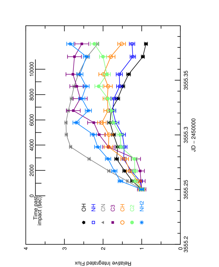
Figure 5: Cochran et al.. 2006

References

- [A’Hearn et al. 2005] A’Hearn, M. F., M. J. S. Belton, W. A. Delamere, J. Kissel, K. P. Klaasen, L. A. McFadden, K. J. Meech, H. J. Melosh, P. H. Schultz, J. M. Sunshine, P. C. Thomas, J. Veverka, D. K. Yeomans, M. W. Baca, I. Busko, C. J. Crockett, S. M. Collins, M. Desnoyer, C. A. Eberhardy, C. M. Ernst, T. L. Farnham, L. Feaga, O. Groussin, D. Hampton, S. I. Ipatov, J.-Y. Li, D. Lindler, C. M. Lisse, N. Mastrodemos, W. M. Owen, J. E. Richardson, D. D. Wellnitz, and R. L. White 2005. Deep Impact: Excavating Comet Tempel 1. Science 310, 258–264.
- [Feldman et al. 2006] Feldman, P. D., R. E. Lupu, S. R. McCandliss, H. A. Weaver, M. F. A’Hearn, M. J. S. Belton, and K. J. Meech 2006. Carbon monoxide in comet 9P/Tempel 1 before and after the Deep Impact encounter Ap. J. (Letters), submitted.
- [Groussin et al. 2006] Groussin, O., M. F. A’Hearn, J.-Y. Li, P. C. Thomas, J. M. Sunshine, C. M. Lisse, A. Delamere, and the Deep Impact Science Team 2006. Temperature of the nucleus of comet Tempel 1. Lunar and Planetary Science XXXVII abstract 1297.
- [Hardorp 1978] Hardorp, J. 1978. The Sun among the stars. I - A search for solar spectral analogs. Astr. and Ap. 63, 383–390.
- [Jehin et al. 2006] Jehin, E., J. Manfroid, D. Hutsemékers, A. L. Cochran, C. Arpigny, W. M. Jackson, H. Rauer, R. Schulz, and J.-M. Zucconi 2006. Deep Impact: High resolution optical spectroscopy with the ESO VLT and the Keck 1 telescope. Ap. J.(Letters) 641, L145–L148.
- [Keller et al. 2005] Keller, H. U., L. Jorda, M. Küppers, P. J. Gutierrez, S. F. Hviid, J. Knollenberg, L.-M. Lara, H. Sierks, C. Barbieri, P. Lamy, H. Rickman, and R. Rodrigo 2005. Deep Impact observations by OSIRIS onboard the Rosetta spacecraft. Science 310, 281–283.
- [Küppers and 40 additional authors 2005] Küppers, M. and 40 additional authors 2005. A large dust/ice ratio in the nucleus of comet 9P/Tempel 1. Nature 437, 987–990.
- [Lisse and the Deep Impact Spitzer Science Team 2006] Lisse, C. M. and the Deep Impact Spitzer Science Team 2006. Spitzer Space Telescope observations of the nucleus and dust of Deep Impact target comet 9P/Tempel 1. Lunar and Planetary Science XXXVII abstract 1960.
- [Meech and 208 additional authors 2005] Meech, K. J. and 208 additional authors 2005. Deep Impact: Observations from a worldwide Earth-based campaign. Science 310, 265–269.
- [Mumma et al. 2005] Mumma, M. J., M. A. DiSanti, K. Magee-Sauer, B. P. Bonev, G. L. Villanueva, H. Kawakita, N. Dello Russo, E. L. Gibb, G. A. Blake, J. E. Lyke, R. D. Campbell, J. Aycock, A. Conrad, and G. M. Hill 2005. Parent volatiles in comet 9P/Tempel 1: Before and after impact. Science 310, 270–274.
- [Porto de Mello and da Silva 1997] Porto de Mello, G. F. and L. da Silva 1997. HR 6060: The closest ever solar twin? Ap. J.(Letters) 482, L89–L92.
- [Schleicher et al. 2006] Schleicher, D. G., K. L. Barnes, and N. F. Baugh 2006. Photometry and imaging reults for comet 9P/Tempel 1 and Deep Impact: Gas production rates, postimpact light curves, and ejecta plume morphology. A. J. 131, 1130–1137.
- [Strazzula and Johnson 1991] Strazzula, G. and R. E. Johnson 1991. Irradiation effects on comets and cometary debris. In Comets in the Post-Halley Era pp. 243–275 Kluwer Academic Press Dordrecht, Netherlands.
- [Sugita et al. 2005] Sugita, S., T. Ootsuba, T. Kadono, M. Honda, S. Sako, T. Miyata, I. Sakon, T. Yamashita, H. Kawakita, H. Fujiwara, T. Fujiyoshi, N. Takato, T. Fuse, J. Watanabe, R. Furusho, S. Hasegawa, T. Kasuga, T. Sekiguchi, D. Kinoshita, K. J. Meech, D. H. Wooden, W. H. Ip, and M. F. A’Hearn 2005. Subaru telescope observations of Deep Impact. Science 310, 274–278.
- [Vogt 1992] Vogt, S. S. 1992. HIRES - a High Resolution Echelle Spectrometer for the Keck Ten-Meter Telescope. In ESO Workshop on High Resolution Spectroscopy with the VLT. Proceedings, held in Garching, Germany, February 11-13, 1992. Editor, M.-H. Ulrich; Publisher, European Southern Observatory, Garching bei Munchen, Germany, 1992. (M.-H. Ulrich, Ed.) pp. 223–.