The Galaxy Mass Function up to z=4 in the GOODS-MUSIC sample: into the epoch of formation of massive galaxies

Abstract

Aims. The goal of this work is to measure the evolution of the Galaxy Stellar Mass Function and of the resulting Stellar Mass Density up to redshift $\simeq 4$, in order to study the assembly of massive galaxies in the high redshift Universe.

Methods. We have used the GOODS-MUSIC catalog, containing $\sim$3000 Ks-selected galaxies with multi-wavelength coverage extending from the U band to the Spitzer $8\mu$m band, of which 27% have spectroscopic redshifts and the remaining fraction have accurate photometric redshifts. On this sample we have applied a standard fitting procedure to measure stellar masses. We compute the Galaxy Stellar Mass Function and the resulting Stellar Mass Density up to redshift $\simeq 4$, taking into proper account the biases and incompleteness effects.

Results. Within the well known trend of global decline of the Stellar Mass Density with redshift, we show that the decline of the more massive galaxies may be described by an exponential timescale of $\simeq 6$ Gyrs up to $z\simeq 1.5$, and proceeds much faster thereafter, with an exponential timescale of $\simeq 0.6$ Gyrs. We also show that there is some evidence for a differential evolution of the Galaxy Stellar Mass Function, with low mass galaxies evolving faster than more massive ones up to $z\simeq 1-1.5$ and that the Galaxy Stellar Mass Function remains remarkably flat (i.e. with a slope close to the local one) up to $z\simeq 1-1.3$.

Conclusions. The observed behaviour of the Galaxy Stellar Mass Function is consistent with a scenario where about 50% of present–day massive galaxies formed at a vigorous rate in the epoch between redshift 4 and 1.5, followed by a milder evolution until the present-day epoch.

1 Introduction

The observational evidence of the continuous increase of the stellar content of galaxies over cosmic times has emerged only recently from a series of observations and surveys which have made use of new sensitive IR instrumentation. Following the first pioneering studies (Giallongo et al. (1998), Brinchmann & Ellis (2000), Papovich et al. (2001)) that set-up the technique for estimating stellar masses in high redshift galaxies, several surveys pointed out that the global stellar content of the Universe, as measured by the average stellar mass density, increases with cosmic time (Brinchmann & Ellis (2000), Dickinson et al. (2003), Fontana et al. (2003), Rudnick et al. (2003), Glazebrook et al. (2004), Drory et al. (2004), Fontana et al. (2004), F04 hereafter, Rudnick et al. (2006)).

While the average stellar mass density provides a global picture of the process of stellar assembly, the Galaxy Stellar Mass Function (GSMF in the following) provides a more detailed view on how this process evolves as a function of the galaxy mass itself. At low redshift, accurate GSMF have been obtained from the 2dF (Cole et al. (2001)) or 2MASS–SDSS (Bell et al. (2003)) surveys. Because of the large area and of the accuracy in the redshift estimate that is needed to compile a GSMF, very few GSMFs have been obtained so far. The MUNICS survey (Drory et al. (2004)) and the K20 survey (F04) first explored the evolution of the GSMF up to $z\simeq 1-2$ in a somewhat complementary fashion. The former adopted a wide, relatively deep sample on a wide area ($\simeq 5000$ objects at $K\leq 19$), mostly relying on photometric redshifts, sampling the GSMF up to $z\simeq 1.5$, while the latter adopted a deeper but smaller sample ($\simeq 500$ objects at $K\leq 20$), with excellent spectroscopic coverage, extending up to $z=2$. In the overlapping redshift ranges, the two GSMF agree quite well, and both analyses suggested a decline in the density of massive galaxies at $z\simeq 1$, of the order of 50-70% with respect to the local value. Recently, Drory et al. (2005) extended such analysis to higher ($z\simeq 5$) redshift, adopting a combination of $I$ and $K$–selected samples.

F04 also pointed out a tentative evidence of a differential evolution of the GSMF, such that massive galaxies appear to evolve less than low mass galaxies, at least up to $z\simeq 1.5$. As we shall show in the following, this trend is also shown by our new data.

Along a different line, evidence has emerged that the GSMF for galaxies of different spectral or morphological types shows a significant evolution, with an increase in the fraction of stellar mass residing in late type galaxies at $z\simeq 1-1.5$ with respect to low redshift (F04, Bundy et al. (2005), Franceschini et al. (2006)).

Although these surveys have already provided a first picture of the evolution of the GSMF, the uncertainties involved in this exercise are still large. In particular, the exploration of the high redshift Universe is still very limited. In several cases, the lack of long–wavelength data hampered the estimate of the stellar mass at high redshift, for which an adequate sampling of the rest frame optical–near infrared part of the spectrum is essential. In addition, the collection of a large sample of high redshift galaxies requires a combination of large areas and deep near–IR observations. For different reasons, all the surveys mentioned above suffer of these limitations, although to a different extent.

In this context, the GOODS-South survey provides an excellent opportunity of improving in a significant way our knowledge of the high–$z$ GSMF. The combination of deep, wide IR observations with Spitzer (in its four channels from 3.5 to 8 $\mu$m) and VLT-ISAAC (in $J$, $H$ and $Ks$), coupled with high quality imaging data in the optical domain (both ACS and VLT–VIMOS), and of a large, extended spectroscopic coverage make the GOODS-South field ideal for this investigation. From this public data set we have obtained a multicolour catalog of faint galaxies, that we named GOODS–MUSIC (GOODS MUltiwavelength Southern Infrared Catalog), that we describe in Grazian et al. 2006a .

In this work we use the GOODS–MUSIC sample to improve the previous estimates of the GSMF in several ways. The most important is that our analysis includes the $3.5-8\mu$m Spitzer observations of the complete $Ks$–selected data set. In addition, it extends to $Ks$ magnitudes deeper than any previous survey, enabling us to obtain a complete sample of galaxies up to $z\simeq 4$, and to measure the slope of the low mass side of the Galaxy Stellar Mass Function up to $z\simeq 1.3$. Compared to our previous analysis of the K20 survey data, the present data set provides a final sample that is 6$\times$ larger than the K20 one, on which we adopt a more sophisticated technique to parametrize the evolution of the Galaxy Stellar Mass Function with a redshift-dependent Schechter fit, that provides interesting clues on the evolution of massive galaxies.

The paper is organized as follows. In Sect.2, after reminding the basic feature of our dataset and of the procedure that we adopt to extract the stellar masses from each galaxy, we discuss how the inclusion of the Spitzer bands affects the mass estimates and highlight the selection effects that will affect our analysis. In Sect.3, we present the basic results of our analysis, namely the Galaxy Stellar Mass Function and the resulting mass density, both in a binned as well as in a parametric fashion. In Sect.4, we compare our basic findings with the prediction of recent theoretical models. Finally, in Sect.5, we focus on the highest redshift range, to discuss the reliability of the photometric redshifts on a few, intriguing objects that might be at very high redshift. The discussion and conclusions are summarized in Sect.6.

All the magnitudes cited below are in the AB system. To scale luminosities and compute volumes we have adopted a “concordance” cosmological scenario with $\Omega_{\Lambda}=0.7$ and $H_{0}=70$ km s^-1 Mpc^-1.

2 Stellar Masses in the GOODS–MUSIC sample

2.1 The Data

We use GOODS-MUSIC, a multicolour catalog extracted from the deep and wide survey conducted over the Chandra Deep Field South (CDFS) in the framework of the GOODS public survey. The procedures that we adopted are described at length in Grazian et al. 2006a . We remind here only the basic features.

The data comprise a combination of images that extend over 14 bands, namely U–band data from the 2.2ESO ($U_{35}$ and $U_{38}$) and VLT-VIMOS ($U_{VIMOS}$), the $F435W$, $F606W$, $F775W$ and $F850LP$ ($Z_{850}$) ACS images, the $JHKs$ VLT data and the Spitzer data provided by IRAC instrument (3.6, 4.5, 5.8 and 8.0 $\mu$m). From this dataset, we have obtained a multiwavelength catalog of 14847 objects, selected either in the $Z_{850}$ and/or in the $Ks$ band. For the purposes of the present work, we will mainly use the $Ks$–selected catalog. This consists of 2931 galaxies (after removal of known or candidate AGNs and Galactic stars), 1922 of which have $U_{VIMOS}$ coverage, 1762 have $H$ coverage, and all have a complete coverage in the remaining 12 bands, most notably including the Spitzer ones. Since the detection mosaics have an inhomogeneous depth, we have divided the $Ks$ sample into 6 independent catalogs, each with a well defined magnitude limit and area, that we use to compute mass functions and mass densities. However, the largest fraction of the sample has a typical magnitude limit of $Ks\simeq 23.5$ that we will adopt for more qualitative arguments.

Colours have been measured using a specific software for the accurate “PSF–matching” of space and ground based images of different resolution and depth, that we have named ConvPhot (De Santis et al 2006). We have cross correlated our catalog with the whole spectroscopic catalogs available to date, from a list of surveys, assigning a spectroscopic redshift to more than 1000 sources. We note that in this work we use a spectroscopic sample that is wider than that presented in Grazian et al. 2006a , thanks to the increased number of spectra publicly available (Vanzella et al. (2006)). Finally, we have applied our photometric redshift code, developed and tested over the years in a series of works (Fontana et al. (2000), Cimatti et al. (2002), Fontana et al. (2003), Fontana et al. (2004), Giallongo et al. (2005)), that adopts a standard $\chi^{2}$ minimization over a large set of templates obtained from synthetic spectral models. The comparison with the spectroscopic sample (Grazian et al. 2006a , Grazian et al. 2006b ) shows that the quality of the resulting photometric redshifts is excellent, with a r.m.s. scatter in $\Delta z/(1+z)$ of 0.03 and no systematic offset.

In summary, the final sample adopted in this work consists of 2931 galaxies, complete to a typical magnitude of $Ks\simeq 23.5$, over an area of 143.2 sq. arcmin, 815 of which with reliable spectroscopic redshift (i.e. 28% of the total sample) and the remaining fraction with well tested 14 bands photometric redshifts.

2.2 Stellar Masses in the Spitzer era

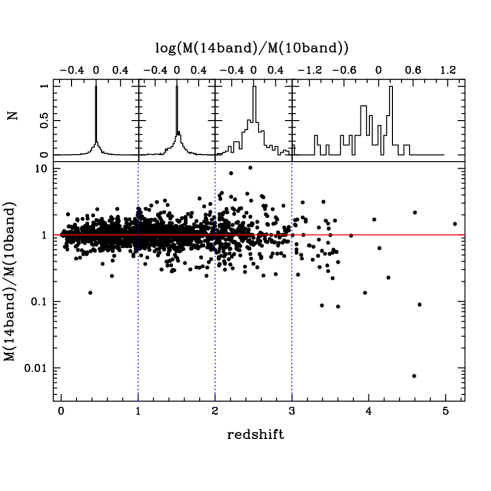
Figure 1: Relation between the stellar masses derived with the inclusion of the Spitzer bands (14 bands) and those without the Spitzer bands (10 bands), as a function of redshift, on the Ks–selected galaxies of the GOODS-MUSIC sample. In the lower panel we plot the ratio between the two estimates, for each galaxy in the $Ks$–selected sample. In the upper, the distribution of such a ratio in different redshift ranges.

The method that we applied to estimate the galaxy stellar masses on this dataset is exactly the same that we developed in previous papers (Fontana et al. (2003), F04), and similar to those adopted by other groups in the literature (e.g. Dickinson et al. (2003), Drory et al. (2004)). Briefly, it is based on a set of templates, computed with standard spectral synthesis models (Bruzual & Charlot 2003 in our case), chosen to broadly encompass the variety of star–formation histories, metallicities and extinction of real galaxies. To compare with previous works, we have used the Salpeter IMF, ranging over a set of metallicities (from $Z=0.02Z_{\odot}$ to $Z=2.5Z_{\odot}$) and dust extinction ($0<E(B-V)<1.1$, with a Calzetti extinction curve). Details are given in Table 1 of F04. For each model of this grid, we have computed the expected magnitudes in our filter set, and found the best–fitting template with a standard $\chi^{2}$ normalization. The stellar mass and other best–fit parameters of the galaxy are found after scaling to the actual luminosity of the observed galaxy. Pros and cons of the method have been discussed in several papers (Papovich et al. (2001), Fontana et al. (2004), Shapley et al. (2004)), and we refer to them for a detailed discussion of the systematics involved in this exercise.

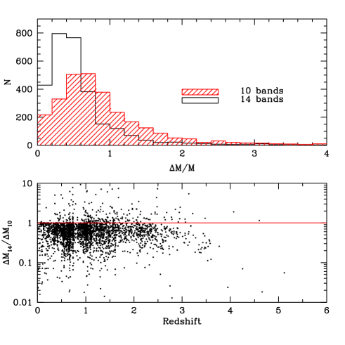
Figure 2: Effect of the Spitzer bands on the mass estimate. Upper panel we plot the distribution of the relative uncertainty (at the $1\sigma$ level) in the mass estimate, when the Spitzer bands are included (14 bands) or not (10 bands). The distribution is computed over all $Ks$–selected galaxies. Lower panel: Ratio of the uncertainty (at the $1\sigma$ level) in the mass estimate, when the Spitzer bands are included (14 bands) or not (10 bands), as a function of redshift.

The major difference with all previous estimates of the GSMF arises from the inclusion of the 4 Spitzer bands, longward of 2.2 $\mu$m. For galaxies at $z>2$, these bands are essential to sample the spectral distribution in the rest-frame optical and near-IR bands, that are necessary to provide reliable constraints on the stellar mass. We quantitatively assess their importance in Fig.1, where we plot the ratio between the mass estimates with (14 bands) and without (10 bands) the Spitzer bands on the sample of $Ks$–selected galaxies, as function of redshift.

It is immediately appreciated that the inclusion of the Spitzer bands does not provide statistically significant changes at $z<2$, where most of the galaxies are fitted with the same best–fitting models in both cases. The scatter in the mass estimate is entirely consistent with the expected uncertainty due to model degeneracy. At higher redshift, the scatter increases significantly. At $z\simeq 2.5$, the r.m.s. fluctuation is of about $0.23$, although with no systematic shift. At higher redshift, the r.m.s. is as large as $0.45$ dex, with evidence of systematic overestimate (of 0.2 dex) of the stellar mass when the Spitzer bands are not included.

The same improvement can be found by looking at the uncertainty in the mass estimate. As in F04, we computed the $1\sigma$ confidence level on each mass estimate by scanning the $\chi^{2}$ levels, allowing the redshift to change in case of objects with photometric redshift. In Fig.2 we compare these estimates when the Spitzer bands are included (14 bands) or not (10 bands). As clearly shown, the formal intrinsic uncertainty decreases from a typical value of 60% to 40% on the global sample, and decreases by a factor of three for objects at $z>2$.

These results confirm that, in the absence of the Spitzer bands, the estimates of the stellar mass for galaxies at $z>3$ are very uncertain and possibly biased, such that detailed astrophysical analysis based on such estimates are likely premature.

2.3 Stellar masses of the GOODS-MUSIC data sample

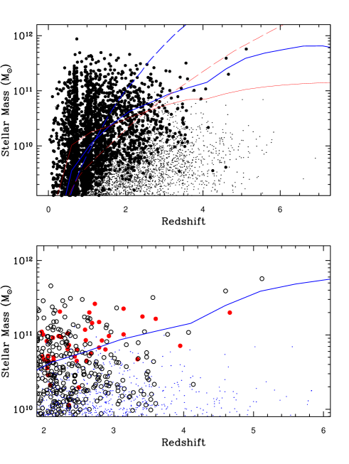
Figure 3: Stellar Masses for individual galaxies of the GOODS-MUSIC sample, as a function of redshift. Upper panel: the $Ks$–selected (filled circles) and the $Z_{850}$–selected sample (small dots) on the overall redshift range. Lower panel: same quantities, for galaxies at $z\geq 2$. Objects in the $Ks$–selected sample are shown with large empty circles if they are also included in the $Z_{850}$–selected one, and with large filled circles if included only in the $Ks$-band catalog. Small dots are from the remaining $Z_{850}$–selected objects. In both panels, lines represent the completeness threshold, computed as described in the text. Thick lines correspond to the completeness threshold for a $Ks$–selected sample with respect to passively evolving models (continuous line) and dusty starburst with $E(B-V)=1.1$ (dashed). The thin lines show the same thresholds if a 4.5$\mu$m–selected sample would be used, for the two same spectral models.

In Fig.3 we plot the resulting stellar masses of the GOODS-MUSIC sample, as a function of redshift. We include in the plot both the objects of the $Ks$–selected sample as well as those of the $Z_{850}$–selected one that have detected flux in the $Ks$ band.

One can immediately appreciate that massive galaxies (i.e. those above the $z=0$ characteristic mass $M_{*}\simeq 10^{11.}M_{\odot}$) are thoroughly detected up to at least $z\simeq 4$, and possibly even at higher $z$, although the reliability of photometric redshifts for the massive objects at $z\simeq 5$ is uncertain, as discussed in Section 5. We also note that such plot appears to be qualitatively different from the analogous plot by Drory et al. (2005), that contains several quite massive galaxies (close to $10^{12}M_{\odot}$) up to $z\simeq 5$. This difference is likely due to a combination of effects, induced by the different techniques applied for photometry and photometric redshifts, the availability of an extended spectroscopic coverage, and probably even more important the lack of Spitzer observations in the Drory et al. (2005) sample.

In the lower panel of Fig.3 we focus on the high redshift range of our sample, and we use different symbols to differentiate among galaxies that are selected only in the $Ks$–selected sample, those that are selected both in $Ks$ and $Z_{850}$ and those that are selected in $Z_{850}$ only. As expected, galaxies that are selected in $Z_{850}$ only, and hence have a very low flux in $Ks$, populate the low mass region of the distribution. On the contrary, a number of galaxies selected only in $Ks$ contribute to the population of massive galaxies at $z>2$: these are typically very faint or sometimes even undetected in the $Z_{850}$–band, resulting from highly dust–reddened or passively fading stellar population at high redshift. These objects significantly contribute to the number density of massive systems. In a similar way, one expects that other massive galaxies at these redshifts might be included by selecting the sample at even higher wavelengths, as those obtained with the Spitzer observations used here.

2.4 Incompleteness and selection criteria

It is important to remark that our sample, as well as any other magnitude -limited sample, does not have a well defined, sharp limit in stellar mass. This incompleteness effect arise from the fact that galaxies have a range of $M/L$ ratios, and can be illustrated as follows. In the GOODS–MUSIC sample, at $z=1$ we find that galaxies have a range of $M/L$ extending from 0.9 (for redder objects) to 0.046 (for bluer objects). Assuming for simplicity a sharp magnitude limit $Ks=23.5$, this corresponds to stellar masses from $M_{\odot}\simeq 1.5\cdot 10^{10}$ (for redder objects) to $M_{\odot}\simeq 6\cdot 10^{8}$ (for bluer objects). However, since galaxies have a range of $M/L$ ratios, additional objects with stellar masses in the range $6\cdot 10^{8}<M_{\odot}<1.5\cdot 10^{10}$ will lay at fainter fluxes, $Ks>23.5$, which are not included in the present sample. Hence, the census of galaxies in the range $6\cdot 10^{8}<M_{\odot}<1.5\cdot 10^{10}$ will definitely be incomplete in our sample, at $z\simeq 1$. A complete visualization of this effect can be obtained by looking at Fig 16 of F04. Needless to say, this effect exists in any magnitude-limited sample and at any redshift, although going to redder wavelengths alleviates its impact.

This effect has been described at length by Dickinson et al 2003, Fontana et al 2003 and F04, and can be dealt with in two different ways. First, one can compute a limiting threshold in mass, such that one can obtain a well defined mass–selected sample. All the relevant statistics (mass densities, mass functions etc) should be obtained using only the objects above such limit in stellar mass.

To better exploit the statistics of the sample, we have developed a technique to correct for the incomplete coverage of $M/L$ ratios, that allows to at least partially recover the fainter side of the sample. This technique will be used to estimate the GSMF and will be described in Sect. 3. In our sample, this technique allows to extend the GSMF by about $0.4dex$ in each redshift bin: the leading effect remains therefore the conservative estimate of the completeness limit, that we have derived as follows.

The limiting threshold in mass can be obtained by computing the maximal $M/L$ that is allowable at each redshift and multiplying it by the magnitude limit of the survey. Below such a threshold in mass, one can still detect galaxies and measure their mass, but will start to miss galaxies of the same mass but with lower luminosity (i.e. higher $M/L$). Unfortunately, such a limiting threshold depends on the assumed spectral properties for the targeted galaxies (and obviously on the bandpass adopted to select the catalog).

In the simplest case, one can compute the maximal $M/L$ for passively evolving systems. In this case, it is easy to draw a selection curve, that we plot in Fig.3 (thick solid line), that we computed with a maximally old, single burst model normalized to $Ks=23.5$. However, large values of $M/L$ can also be found in heavily extincted star–forming galaxies. To estimate this effect, we have adopted a simple star–forming model with a variable amount of extinction, adopting a Calzetti extinction law. It turns out that, for $E(B-V)\simeq 0.5$, the corresponding selection curve roughly corresponds to the “passively evolving” one, and we do not plot it for simplicity. Increasing the amount of dust, the selection curve shifts to higher masses. In Fig.3 we plot the case for $E(B-V)\simeq 1.1$ (thick dashed line), that is among the highest observed in spectroscopically confirmed EROs (Cimatti et al. (2002)).

The result must be read as follows: our $Ks$–selected sample is expected to be complete against passively evolving objects with mass above the thick solid line in Fig.3, i.e. grossly with mass $M_{*}\geq 10^{11}M_{\odot}$ up to $z\simeq 4$; however, at this mass level it becomes progressively biased against the detection of extremely dusty objects, probably already at $z\geq 2$.

It is interesting to predict what would be the advantages of adopting a Spitzer–selected sample, scaled to the expected sensitivity of the GOODS survey. We have computed the same selection curves (for passively evolving and dusty objects) adopting a magnitude limit at $4.5\mu$m of $m_{4.5}\leq 23.5$, and we have overplotted them in Fig.3 as thin solid and dashed lines. A first result is that the adoption of a $4.5\mu$m–selected sample would not allow to extend the sampling of passively evolving galaxies at lower masses than in our catalog, but rather to extend the selection of objects at the same level of $M_{*}\simeq 10^{11}M_{\odot}$ well beyond $z\simeq 4$. Probably the most important effect is that the adoption of a $4.5\mu$m–selected sample would allow the detection of heavily extincted, dusty objects well beyond $z\simeq 2$, probably up to $z\simeq 3$ at the $M_{*}\simeq 10^{11}M_{\odot}$ level. Objects detected in the $4.5\mu$m band, but very faint or even undetected in $Ks$, do exist in the GOODS area (see Yan et al 2005 for a few cases): unfortunately, their inclusion in the present analysis would require a detailed analysis (most notably of the reliability of their photometric redshift), that would go beyond the purposes of this work and that we defer to a dedicated paper.

3 The Galaxy Stellar Mass Function

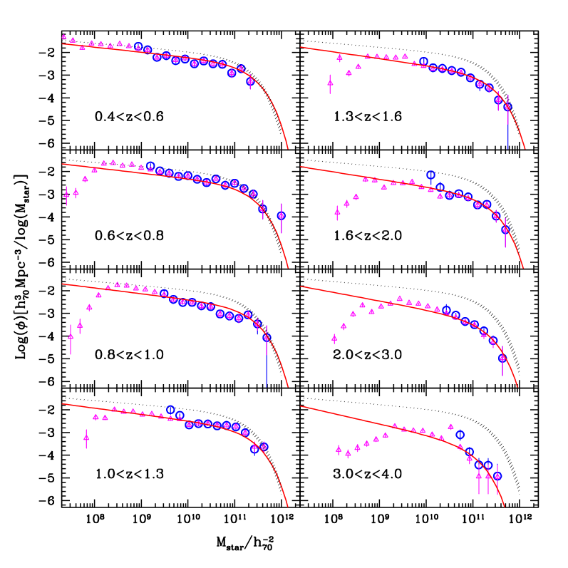
Figure 4: Galaxy stellar Mass Functions in the GOODS–MUSIC sample, in different redshift ranges. Big circles represent the Galaxy Stellar Mass Functions of the $Ks$–selected sample, computed with the $1/V_{max}$ formalism up to the appropriate completeness level, as described in the text, while small triangles show the Galaxy Stellar Mass Functions of the $Z_{850}$–selected sample, computed without any correction for incompleteness coverage of the $M/L$ at faint limits. The dashed region represents the local GSMF of Cole et al. (2001), encompassing its original and the “rescaled” version that we obtained in F04 (see text for details). The solid line is the evolutionary STY fit of our data, computed over the global redshift range $0.4<z<4$, that we describe in Section 3.2. The observed mass functions are available in electronic form at http://lbc.oa-roma.inaf.it/goods/massfunction.

3.1 Computing the Mass Function

We have used the $Ks$–selected sample described above to compute the GSMF at various redshifts. The GSMF is computed both by using the standard $1/V_{max}$ formalism as well as by fitting a Schechter function to the unbinned data. The results of the former method are described in Sect. 3.2, while the latter in 3.3.

The GSMF must be computed taking into account the incompleteness effects described above. To correct for this effect, we have introduced a correction technique, which is carefully described in F04, and that we remind briefly here. We start from the threshold computed from passively evolving system, i.e. the thick solid line of Fig.3: below such completeness threshold only a fraction ($f_{\rm obs}$) of objects of given mass will be observed. We then obtain (at any redshift) the observed distribution of $M/L$ ratios for objects close to the magnitude limit of the sample. Then, using such distribution, we compute for each mass and redshift the fraction $1-f_{\rm obs}$ of galaxies lost by effect of the incomplete coverage of the $M_{*}/L_{K}$ ratio, by which we obtain $f_{\rm obs}$. As shown in F04, Appendix B, relatively simple analytic formulae can be used to describe this process. We adopted the same technique to the GOODS-MUSIC sample, verifying that these simple analytic expression still provide a good fit to the observed $M_{*}/L_{K}$ distribution, despite the greater depth and area of the GOODS-MUSIC sample. The correction is applied only for a limited range of masses, where the correction is less than 50% (i.e. $f_{\rm obs}\geq 0.67$. This correction factor is then applied to the volume element $V_{\rm max}$ of any galaxy in the $1/V_{\rm max}$ binned GSMF as well as in the number of detected galaxies that enters in the Maximum Likelihood analysis used to obtain the Schechter best-fits. As shown in Fig. 17 of F04, the inclusion of this treatment allows to extend the computation of the GSMF to somewhat ($0.4dex$) smaller masses than by adopting the strict completeness limit. In contrast, neglecting the whole treatment of incompleteness introduces a remarkable and unphysical bending of the GSMF at low masses.

A further somewhat technical point is related to the choice of the local GSMF that is used to estimate evolution. As described in F04, the parameter grid used as input to the spectral synthesis model adopted here is different from the one adopted in the derivation of the local GSMF by Cole et al. (2001), in particular for the absence of any constraint on the galaxy ages. This systematic difference may lead to a small but systematic bias in the measure of galaxy masses, that can be described by an average relation ($\log(M)=1.027*\log(M_{cole})-0.3955$). By applying this relation to the original Cole et al. (2001) local GSMF we obtain a “rescaled” version of the local GSMF, where differences are in practice noticeable only on the exponential tail of the GSMF. For sake of clarity, we will in the following represent both the original Cole et al. (2001) local GSMF as well as its rescaled form that we derived in F04.

3.2 The distribution of massive galaxies up to z$\simeq 4$

The Galaxy Stellar Mass Function obtained in the GOODS–MUSIC sample is shown in Fig.4, where it is computed in several redshift bins. We also plot in Fig.4 the GSMF obtained on the $Z_{850}$–selected sample, naively computed with no correction for the incomplete coverage of the $M/L$ distribution. We explicitly note that such a $Z_{850}$–selected GSMF is quite consistent with the $Ks$–selected one at low and intermediate redshifts, before fading at the lowest mass end because of the lack of correction for incompleteness. Conversely, it misses a significant fraction of massive galaxies at $z>2-3$, as expected in a $Z_{850}$–selected sample.

We also remark that the error bars of Fig.4 have been computed with a full Monte Carlo simulation where we take into account the redshift probability distribution of each galaxy in the sample.

Three different results can be inferred even from a visual inspection of Fig.4. First, the density of massive galaxies clearly decreases with redshift, relatively mildly up to $z\simeq 1.5$ and then much more convincingly at $z>2$. At $z\simeq 3.5$, their density is at least a factor 10$\times$ lower than in the local Universe. This result confirm the trend that we already noted in F04 (see also Drory et al 2005).

Second, the number density of lower mass system evolves significantly with redshift (at $z\simeq 1$ the density of galaxies with $M\simeq 10^{10}M_{\odot}$ is 4 times lower than the local one), while the slope of the GSMF is relatively flat up to at least $z\simeq 1-1.5$, and does not appear to steepen significantly with respect to the local one. The latter result is apparently at variance with the results of in F04, where we found a significant steepening of the GSMF at $z\simeq 0.7$, with the slope index $\alpha$ changing from $\alpha=-1.18$ at $z=0$ to $\alpha=-1.4$ at $z=0.7$. We first carefully checked that no systematic effect is responsible for this result: in particular, we verified that the GSMF computed with our new sample in the very area of the K20 survey is comparable to our early results (actually it is nearly perfectly coincident), despite the new photometry of the whole sample. We furthermore note that even in the GOODS–MUSIC sample the slope of the GSMF is steeper than the average in the redshift bin $z=0.8-1$, as also shown by the parametric analysis presented in Sect.3.3, probably due to a cosmic variance effect. Taking also into account the agreement with the $Z_{850}$–selected GSMF, we conclude that our new sample, that is much deeper and wider than the K20 sample, allows to better represent the global evolution of the slope of the GSMF with redshift.

Finally, there is some evidence of a differential evolution of the GSMF, in the sense that more massive galaxies appear to evolve less than low mass galaxies, at least up to $z\simeq 1.5$. This trend was already noted in F04, but the more limited statistics prevented a robust quantitative conclusion.

Although these conclusions are clearly supported by our data, we are aware that the $1/V_{max}$ approach is very sensitive to the biases induced by Large Scale Structures (LSS) and clustering, and that our sample is clearly affected by these effects. A well known effect is the apparent steepening of the faintest points in case of clustering (Heyl et al. (1997)): this is present in our sample at $1<z<1.3$ and $1.6<z<2$, due to two large overdensities at the lower limit of the bin. Such effects are amplified by the arbitrariness in the choice of the redshift bins, and by our choice of keeping a small binning factor in mass. If one compares our sample with the local GSMF of Cole et al. (2001), it is possible to see that fluctuations in the number of massive galaxies exist, superimposed to the global evolution of the GSMF. In particular, the number of massive galaxies and even the detection of galaxies with $M_{*}>10^{11}M_{\odot}$ is higher in the redshift bins where LSS have been detected in the CDFS field, e.g. at $z=0.67,0.73$, $z\simeq 1.61$ (Gilli et al. (2003), Vanzella et al. (2005), Vanzella et al. (2006)), while our sample is relatively devoid of massive galaxies at $z\simeq 0.9$, where an underdensity of galaxies exists in the CDFS (Perez–Gonzales et al (2005)). To overcome these limitations, we have developed the STY analysis that we shall describe in the following section.

3.3 The STY approach

An independent approach to the evaluation of the GSMF is the STY fitting method (Sandage et al (1979)), mutuated from the corresponding formalism of the Luminosity Function. This method assumes an analytic expression of the GSMF and derives the free parameters with a Maximum Likelihood analysis. It is less sensitive to clustering and LSS and provides more quantitative hints on the evolution of the global population. To minimize the impact of LSS, and to avoid any arbitrariness in the definition of the redshift bins, we use here a global, redshift-dependent parametrization of the GSMF. At each redshift, the number density $\phi(M,z)$ of galaxies with mass $M_{*}$ is assumed to have the functional form of a Schechter function,

$$\phi^{*}(z)\log{(10)}[10^{(M-M^{*}(z))}]^{(1+\alpha^{*}(z))}\exp(-10^{(M-M^{*}(z)}))$$ (1)

where $M=log_{10}(M_{*}/M_{\odot})$ and the free parameters $\phi^{*}(z)$, $\alpha^{*}(z)$ and $M^{*}(z)$ are functions of redshift. For these parameters, we have found that the following simple relations provide an adequate fit to the overall evolution, in the redshift range $0.4\leq z\leq 4$:

$$\phi^{*}(z)=\phi^{*}_{0}\cdot(1+z)^{\phi^{*}_{1}}$$ (2)

$$\alpha^{*}(z)=\alpha^{*}_{0}+\alpha^{*}_{1}\cdot z$$ (3)

$$M^{*}(z)=M^{*}_{0}+M^{*}_{1}\cdot z+M^{*}_{2}\cdot z^{2}\\$$ (4)

where $\phi^{*}_{0}$, $\phi^{*}_{1}$, $\alpha^{*}_{0}$, $\alpha^{*}_{1}$, $M^{*}_{0}$, $M^{*}_{1}$, $M^{*}_{2}$ are free parameters.

In this formalism, the three zero-th order parameters ($M_{0}^{*}$, $\phi_{0}^{*}$ and $\alpha_{0}^{*}$) should ideally reproduce the local values, as estimated for instance by Cole et al. (2001). For this reason we fixed the local characteristic mass and slope to the local values of Cole et al. (2001) and derived the other parameters. The resulting fit is displayed in Fig.4 as a solid line, and the relevant parameters are listed in Table 1. The Maximum Likelihood analysis allows also to perform an estimate of the error budget on the fitted parameters: we show in Fig.5 the $1\sigma$ and $3\sigma$ contour levels on each pair of free parameters, obtained after marginalization of the other parameters. It is clearly shown that all parameters are reasonably well constrained, in particular those ($M^{*}_{1},M^{*}_{2}$ and $\alpha^{*}_{1}$) that are more important for the physical conclusions that we will draw in the following. The resulting evolution with redshift of the characteristic mass $M^{*}(z)$ and of the slope $\alpha^{*}(z)$ is shown in Fig.6, where they are also compared with the corresponding values obtained by a Schechter fit within each redshift bin.

A first robust result of the STY analysis is that the slope of GSMF is remarkably flat and with a small redshift evolution: up to $z\simeq 1-1.3$, the highest redshift where the slope is reliably measured in our sample, the slope $\alpha$ changes of about $0.1$ in our fiducial best–fit model. As discussed before, this is accompanied by a sensible decrease in the number density of low mass galaxies, that for galaxies with $M\simeq 10^{10}M_{\odot}$ is 4 times lower than the local one.

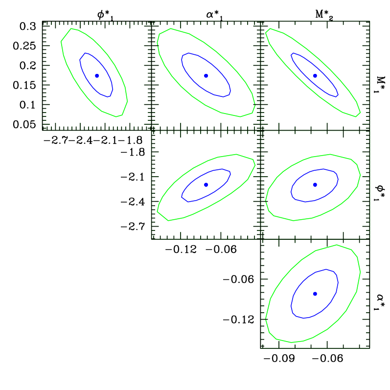
Figure 5: Contour levels of all the pairs of free parameters involved in the Schechter fitting of the GSMF, as obtained by a Maximum Likelihood minimization. Inner ellipses represent the $1\sigma$ contour, outer ones the $3\sigma$ contour. All contours have been obtained with marginalization of the other free parameters.

Figure 6: The evolution of the Schechter parameters $M^{*}$ (characteristic mass) and $\alpha$ (slope) as a function of redshift. Points represent the individual fits to the single redshift bin of Fig.4 with their uncertainty, while lines represents the evolutionary STY fit of our data, computed over the global redshift range $0.4<z<4$, that we describe in Section 3.2. Solid line is the second-order form for $M^{*}$ (our fiducial model); dashed line is for $M^{*}=M^{*}_{1}\times z+M^{*}_{2}\times z^{M^{*}_{3}}$; dotted line is for $M^{*}\propto\log(1+z)$.

The evolution of the characteristic mass $M^{*}(z)$ is more complex. According to the best–fit values, the evolving $M^{*}(z)$ is fitted with a second order law with negative curvature ($M^{*}_{2}=-0.07\pm 0.02$) and a peak at about $z\simeq 1.35$, such that the characteristic mass of the GSMF initially increases, reaches a maximum around $z\simeq 1.35$ and than decreases.

We carefully verified that this behaviour is not a spurious result of our choice of the functional form of Eq.4, where the second order law for $M^{*}(z)$ might introduce such a non-monotonic behaviour. First, as shown in Fig.5, the second order term $M_{2}$ is definitely negative, suggesting that $M^{*}(z)$ actually increases up to $z\simeq 1-1.3$ and decreases thereafter. Such a behaviour is also consistent with the trend observed in the values of $M^{*}$ in the individual redshift bins, as shown in Fig.6. More important, we arrived at this choice after discarding simpler solutions. In particular, we tested a linear form for $M^{*}(z)$ (i.e. with $M_{2}^{*}=0$), as well as a more traditional logarithmic function ($M^{*}(z)=M^{*}_{0}+M^{*}_{1}\cdot\log(1+z)$). The output of the latter form is also shown in Fig.6. In all these cases, we were not able to fit the massive side of the GSMF at intermediate redshifts ($0.6\leq z\leq 1.5$), that is systematically underfitted, by nearly 50%. As a further test, we have also allowed for the exponent of the high order term to be free (i.e. $M^{*}(z)=M^{*}_{0}+M^{*}_{1}\cdot z+M^{*}_{2}\cdot z^{M^{*}_{3}}$), and found that it is definitely larger than 1 ($M^{*}_{3}=1.2\pm 0.05$), providing an evolution that is similar to our fiducial model, as shown by the dashed line in Fig.6. We conclude that such evolutionary form is a robust property of our sample, and we shall adopt the second order form for $M^{*}(z)$ shown in Eq. 4 as our best–fit fiducial model.

Other warnings arise from possible biases in our sample. The most obvious sources of biases are sample variance and the use of photometric redshifts for a relatively large fraction of the sample. We expect the latter uncertainty to be minor, given the large spectroscopic coverage of the GOODS survey for the brightest galaxies (where most of the evolution of $M_{*}$ is measured) and the good accuracy that we achieve in photometric redshifts. Sample variance is a more serious concern, since the GOODS–South field is definitely too small to avoid spurious effects due to over- and under-densities along the line of sight. In the redshift interval $0.6<z<1$ a range of different densities exist, from overdensities (around $z=0.7$) to underdensities (at $z\simeq 0.9$), and the increase of $M^{*}$ is reassuringly seen in both. However, much wider surveys with comparable depth are definitely required to confirm or dispute our finding.

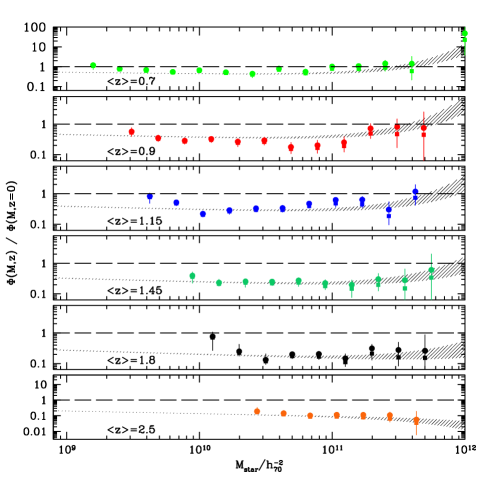
Figure 7: Ratio between the observed Galaxy Stellar Mass Functions in the GOODS–MUSIC sample and the local GSMF, in the same redshift bins of Fig.4. The observed data are normalized to two different choices of the local GSMF, namely the original one of Cole et al. (2001) (filled squares) and its rescaled version, that we described in the text (filled circles). The shaded area shows the corresponding ratios for the global Schechter fit, that we describe in Sect. 3.2.

Turning to physical interpretation of this result, we remark that the evolution of the characteristic mass $M_{*}$ reflects an evolution of the shape of the GSMF, that is progressively skewed toward larger masses as it evolves from $z=0$ to $z\simeq 1.3$. The parametric analysis of this section enforces what we already highlighted in Sect.3.2, i.e. that the GSMF appear to have a differential evolution, with more massive galaxies evolving less than low mass galaxies, up to $z\simeq 1-1.3$. We note that this does not imply that the mass density increases, since the increase of $M^{*}(z)$ is counterbalanced by a decrease of the overall normalization $\phi^{*}(z)$.

The issue of the differential evolution of the GSMF is potentially very important, since it is directly related to the “downsizing” scenario for galaxy evolution, such that it is worth a more careful examination. We plot in Fig.7 the ratio between our GSMF and the local one, for different redshifts. In addition to the obvious overall evolution of the GSMF with redshift, it is shown that the density of galaxies above $10^{11}M_{\odot}$ - albeit decreasing - remains closer to the local value up to $z\simeq 1.15$ than that of the lower mass population. Such a trend appears to be progressively stronger for the more massive galaxies of our survey, i.e. those with a stellar mass in excess of $3\times 10^{11}M_{\odot}$. At larger redshifts, however, this trend eventually breaks down, such that the density of massive galaxies undergoes a strong evolution in the redshift range $1.5<z<3$.

3.4 The integrated Stellar Mass Density

A more global view on the rise of the galaxy mass as a function of cosmic time is provided by the Stellar Mass Density (SMD), that is obtained by integrating the GSMF over all masses (we choose in particular to integrate from log$(M_{*}/M_{\odot})=8$ to log$(M_{*}/M_{\odot})=13$). This is displayed in Fig.8, where we plot as a solid line the SMD as obtained by integrating our Schechter fiducial model. At $z>1.3$, where we do not adequately sample the faint end of GSMF, we rely on the extrapolation of the slope $\alpha$ provided by our fiducial model, that corresponds to a very mild steepening with redshift. In Tab.2 we provide the SMD values as obtained by integrating the Schechter fits as well as those directly observed. When compared also with other surveys, Fig.8 depicts a scenario where the global stellar mass density has evolved relatively slowly (i.e. by a factor of two) over the last 8 Gyrs, and more rapidly at higher redshift, with a decrease by an order of magnitude at $z\simeq 3$.

A more direct result of our survey is the SMD in massive galaxies, defined as those above $M=10^{11}M_{\odot}$, that we directly detect in our survey up to $z\simeq 4$.

As we show in the lower panel of Fig.8, the evolution of the stellar mass density of massive galaxies increases fastly over the first 3-5 Gyrs in the history of Universe, and thereafter proceeds at a much slower pace. It is possible to grossly reproduce this behaviour by an exponential law, $\rho(z)\propto e^{-t/\tau}$, characterized by two different e-folding timescales. At high redshift ($z>1.5$, i.e. look back time $>9$ Gyrs), the timescale that we derive from our data is of the order of $0.6$ Gyrs. At later cosmic times, the timescale is at least a factor of 10 larger: we obtain 6 Gyrs from $z=0$ to $z=1.5$.

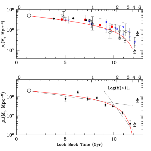
Figure 8: Global Stellar Mass Density as function of redshift. Upper panel: the total Stellar Mass Density (integrated from log$(M_{*}/M_{\odot})=8$ to log$(M_{*}/M_{\odot})=13$) as estimated in the present work, obtained by an integration of our fiducial Schechter function (solid line). It is compared with other estimates adopted from the literature: the local value by Cole et al. 2001 (large empty circle), Fontana et al. 2004 (red filled circles), Fontana et al. 2003 (HDFS, open diamonds), Dickinson et al. 2003 (open squares), Cohen et al. 2001 (open crosses), Brinchmann and Ellis 2000 (filled diamonds), Drory et al. 2005 (open triangles, K-selected sample with horizontal basis, I-selected sample with vertical basis). To avoid further confusion, we do not plot here the mass density computed in this paper. It is useful to stress that the solid curve is not a fit to these data, but only our best parameterization of the SMD in the GOODS-MUSIC sample, which agrees well with that of Fontana et al. 2004 in the K20 region and with Drory et al. 2005 on the GOODS-South field. Lower panel: the mass density computed only on galaxies more massive than log($M_{*}/M_{\odot})=11$. We remark that the value at $z\simeq 0.5$ is affected by an undersampling of massive galaxies because of the small size of the volume element. The solid line shows the mass density computed with our fiducial Schechter fit. See text and Tab.1 for details. The two dotted lines represent an exponentially declining evolution of the stellar mass density, with timescales $\tau 6,0.6$Gyrs obtained by fitting the data at $z<1.5$ and $z>1.5$, respectively.

Table 1: Best fit Schechter parameters

$M^{*}_{0}$	$11.16$
$M^{*}_{1}$	$+0.17\pm 0.05$
$M^{*}_{2}$	$-0.07\pm 0.01$
$\alpha^{*}_{0}$	$-1.18$
$\alpha^{*}_{1}$	$-0.082\pm 0.033$
$\phi^{*}_{0}$	$0.0035$
$\phi^{*}_{1}$	$-2.20\pm 0.18$

Table 2: The Stellar Mass Density

$<z>$	Schechter	Observed	Schechter	Observed
	$8<\log{(M/M_{\odot})}<13$		$\log{(M/M_{\odot})}>11$	$\log{(M/M_{\odot})}>11$
0.50	8.46	$8.32^{+0.03}_{-0.03}$	8.10	$7.89^{+0.13}_{-0.13}$
0.70	8.37	$8.53^{+0.02}_{-0.02}$	8.01	$8.24^{+0.07}_{-0.07}$
0.90	8.29	$8.16^{+0.03}_{-0.03}$	7.93	$7.90^{+0.10}_{-0.11}$
1.15	8.18	$8.26^{+0.02}_{-0.02}$	7.83	$7.94^{+0.06}_{-0.06}$
1.45	8.07	$7.96^{+0.03}_{-0.03}$	7.70	$7.57^{+0.09}_{-0.09}$
1.80	7.94	$7.90^{+0.04}_{-0.04}$	7.54	$7.50^{+0.09}_{-0.09}$
2.50	7.68	$7.60^{+0.04}_{-0.04}$	7.19	$7.16^{+0.08}_{-0.08}$
3.50	7.27	$7.23^{+0.12}_{-0.12}$	6.48	$6.60^{+0.16}_{-0.17}$
4.50		$7.73$		$6.44$
5.50		$7.84$		$7.71$

The Stellar Mass Density at different redshift bins: the second column shows the fitted SMD (integrated from log$(M_{*}/M_{\odot})=8$ to log$(M_{*}/M_{\odot})=13$), the third the observed SMD, while the fourth and the fifth columns are the fitted and observed SMD for log$(M_{*}/M_{\odot})>11$.

4 The comparison with theoretical $\lambda$–CDM models

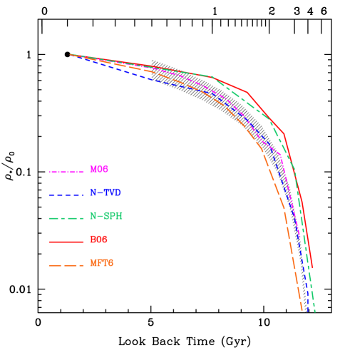
Figure 9: Comparison between the observed Stellar Mass Density in massive galaxies (defined as those above $M_{*}>10^{11}M_{\odot}$) and the corresponding predictions by recent theoretical models, as a function of redshift. Both data and models have been normalized to their own corresponding local value, for the relevant IMF. The shaded area represent the data obtained in the present work, normalized with two different choices of the local mass function (see text for details). The other curves show the prediction of theoretical models, as labelled in the legend: Bower et al. (2006) (B06), Menci et al. (2006) (M06), Monaco et al. (2006) (MFT06), Nagamine et al. 2005a (N-TVD), Nagamine et al. 2005b (N-SPH).

In this section we compare our data with a set of recent theoretical predictions. In particular, we have included in the comparison three recent semianalytic models that include the feedback from AGNs on galaxy formation, albeit with different recipes. The first is the latest rendition of the semianalytical Durham model (Bower et al. (2006), B06 hereafter), where the feedback from AGNs is ignited by the continuous accretion of gas on the central black hole. Such an implementation is conceptually different from the Menci et al. (2006) model (M06 in the following), where the feedback from AGN is explicitly due to the blast wave originated during the active (luminous) phase of AGN activity. Differences between these two models are better detailed in Menci et al. (2006). Finally, in the semianalytic model of Monaco et al. (2006) (MFT06) cooling, infall, star formation, feedback, galactic winds and accretion onto black holes are described with a set of new simplified models that take into account the multi-phase nature of the ISM and its energetics. In particular, the quenching of late cooling flows results from the injection of energy from massive black holes that accrete slowly (in Eddington terms) from the cooling flow itself. A completely different approach is provided by the hydrodynamical simulations in a cosmological context of Nagamine et al. 2005a , Nagamine et al. 2005b (and references therein), which have been obtained either with a Eulerian mesh code with Total Variation Diminishing (Ryu et al. (2003)) shock capturing scheme (N-TVD in the following) or with a SPH “entropy formulation” method (Springel et al. (2002), N-SPH in the following). Both models include radiative cooling and heating, uniform UV background, supernova feedback and standard recipes for star–formation. In addition, the SPH simulation also include the effects of feedback by galactic winds and a multiphase ISM, that provides a more accurate modelling of the star–formation process.

We first compare these models with one main result of our analysis, the evidence that the evolution of massive galaxies is relatively mild up to $z\simeq 1.5$ and then remarkably faster. At this purpose, we plot again in Fig.9 the evolution of the stellar mass density in massive galaxies as a function of redshift, normalized to the local one, both in our data and in the models.

Since we want to focus on the qualitative behaviour of both model and data, and in order to minimize the impact of different IMFs, we have normalized each model to its predicted value at $z=0$, and for the models with a Kennicutt IMF we have used the corresponding characteristic mass $M_{*}$ at $z=0$.

Fig.9 clearly shows that all models reproduce the observed trend in the evolution of the stellar mass density, with a slow, steady decay up to $z\simeq 1.5$ and a much faster decay thereafter. For all models, the formation of massive galaxies is therefore occurring at a fast pace at $z\geq 1.5-2$, and at slower rate at lower redshift, in broad agreement with the observed evolution. It has to be remarked, however, that the fraction of stellar mass assembled in the high redshift phase varies by a factor of two among the different models, on which we shall comment later.

The other important result of our analysis is that there is a significant evolution in the density of low mass galaxies, that at $z\simeq 1$ are about 40% of the present–day number, and that the GSMF is remarkably flat up to $z\simeq 1-1.3$, with a small evolution of the slope ($\Delta\alpha=-0.1$) with respect to the local value. A comparison with the models for this specific feature is provided in the upper panel of Fig.10, where we plot the GSMF in a broad redshift bin around $z\simeq 1$. It is shown that all the models have an unsatisfactory fit to the data, on the faint side. Most of them fail to fit the relatively large evolution in the density of low mass galaxies, with the result of overpredicting their number. In addition, some of them, and in particular the M06 one, predict a slope of the GSMF much steeper than observed. All these results confirm that the observed flatness of the GSMF and most of all the significant density evolution at intermediate redshifts is a critical feature, difficult to reproduce by current theoretical models.

We also notice that, always at $z\simeq 1$, most of the models roughly predict a correct number of massive galaxies, with the exception of the two hydrodynamical simulations. The consequence of this comparison is that the ratio between massive and low mass galaxies (whose evolution provides the “downsizing” scenario) is not reproduced by any model: it is interesting to remark that such a failure is due to the overprediction of low mass galaxies, and not to an underprediction of massive galaxies.

In the bottom panels of Fig.10 we also compare the theoretical GSMFs to the observed ones in the highest redshift bins. The comparison in the redshift range $2<z<3$ is probably the most statistically meaningful, albeit anyway limited to the higher mass regime, and we briefly concentrate on it. It is shown that, at variance with the overall agreement found at $z\simeq 1$, the considered model span a wide range of predicted densities. Typically, hydrodynamical models tend to overpredict the observed data, while the semianalytical renditions appear to be closer to the data. In the detail, those that include a “QSO-like” feedback from AGNs (M06 and MFT06) tend to underpredict the data, and those with a “radio-like” AGN feedback (B06) tend to overpredict the data. While the disagreement is apparently large (by nearly an order of magnitude) as far as the number densities are concerned, it must be remarked that the effect is emphasized by the steep slope of the exponential tail of GSMF, since the offset in mass between the theoretical predictions and the data is within a factor of two. Since hydrodynamical models do not include feedback from AGNs, while “QSO-like” feedback from AGNs is particularly efficient in massive halos at high redshift, it is tempting to ascribe the difference to this specific feature, although many details of the galaxy formation models, especially the cooling and infall of gas in the infall-dominated halos at high redshift, may play a fundamental role as well.

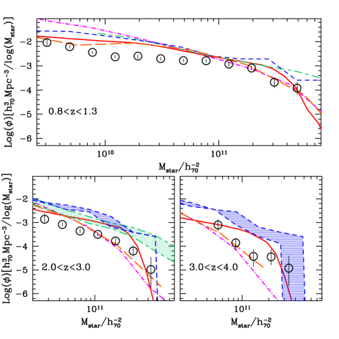
Figure 10: Comparison between the observed GSMF and a set of recent theoretical models. As in Fig.4, large circles represent the mass–complete, Ks–selected sample. Lines refer to different models, as in Fig.9. The dashed areas represent the confidence regions of the models by Nagamine et al 2005ab, where the limits are the predicted mass functions calculated at $z=2$, $z=3$ and $z=4$.

5 Massive galaxies at $z>4$

As we have described in the previous sections, our statistical analysis is limited to $z<4$ to take into full account the various effects of incompleteness in the sample. However, as clearly shown in Fig.3, our sample includes several galaxies at $z>4$. Some of these are “drop–out galaxies”, that are brighter than $m_{z}=26$ and detected in $Ks$, the two requirements that we adopted in plotting Fig.3. As such, our sample does not include many other “I drop–out galaxies”, likely at $z>5$, that are detected in the GOODS images, since they are either fainter than $m_{z}=26$ or undetected in $Ks$. These objects do not make up a complete sample and are therefore excluded from our current analysis.

Most notably, however, we have a few very massive candidate galaxies at $z>4$ in our sample. It is interesting and worthwhile to carry on a detailed analysis of these objects, especially because they give a significant contribution to the mass density of galaxies. In fact, when we estimate the stellar mass density for the galaxies with $z>4$ (Fig.8), we note that it is very high, despite it is a lower limit: this is more evident in the lower panel of the figure where only the mass density of the very massive galaxies is shown. Few very massive galaxies are responsible for such high value of the mass density: at $z=3-4$ two massive galaxies give $34\%$ of the total mass density, while at $z=5-6$ the mass density of only three objects is $94\%$ of the total value.

It is interesting to investigate what kind of objects are these. If we select the galaxies with log$(M_{*}/M_{\odot})>11$, we find three objects, as shown in Fig. 3; two of them are Ks and $Z_{850}$-selected, and one is only Ks-selected. These objects are typically quite red for their redshifts, with a rest–frame $U-V\sim 1.5$. The best-fitting templates for these objects are either passively evolving models, characterized by a very short timescale for star formation $\tau$ with $E(B-V)\sim 0$ or by a constant star formation model with large amount of dust, $E(B-V)>0.5$. Two of these objects are displayed in the left panel of Fig. 11. It is important to stress that the redshift determinations of all these objects are very uncertain, as it is shown by the $\chi^{2}$ as a function of redshift in the same figure. In practice, on the basis of the available data one can only conclude that these objects are most likely at $z>2$, but a sound redshift determination is not available. In particular, other redshift solutions can be find with a similar probability at $z=2-3$.

We note that these objects might resemble the object presented in Mobasher et al. 2005, that is also a candidate massive, passively evolving galaxy at $z\simeq 6.5$. We have also extracted from our raw catalog the photometry of the Mobasher et al. (2005) object (that is slightly fainter than our limiting magnitude in $Ks$), to check how it is classified with our photometry, that is based on a different image set (Mobasher et al. (2005) used a combination of UDF images taken with ACS and NICMOS). With our photometry, such an object is quite similar to our $z\simeq 2$ candidates in Fig. 11, with a flat probability distribution for the photometric redshift from $z=2$ to $7$ and the best fit solution at $z=2.25$ with $E_{B-V}=1.1$: in this case the stellar mass turns out to be $2\cdot 10^{11}M_{\odot}$, quite typical at this redshift.

At this point, it is interesting to seek for similar galaxies in the GOODS–MUSIC sample, i.e. galaxies that have a comparable spectral distribution, best-fitting template around $z=2-3$ and with a probability distribution extending up to $z\simeq 5-6$. Such objects indeed exist in our sample: we find in total three objects, a number comparable to the number of the massive object at higher redshift. Two of them are shown in the right panel of Fig. 11. The fraction of objects with uncertain redshifts is negligible at $z=2-3$ where we have estimated MF and mass density, such that we do not expect that they introduce a significative uncertainty in the statistical analysis. In any case, the effect of such uncertainty is taken into account by the Monte Carlo estimate of the error budget in the GSMF.

We can draw two different conclusions from this exercise. First, although we cannot exclude that some of these objects are actually very massive galaxies at $z>4$, we have to await for a more robust determination of their redshift before including them in a firm estimate of the stellar mass density at high redshift.

Second, the properties of the GSMF can give some hints on the nature of these objects. Probably the most important result of our analysis is that we can exclude that these objects are typical in a statistical sense. Our sample is indeed complete for passively evolving galaxies of stellar mass $M_{*}>10^{11}M_{\odot}$ up to $z\simeq 4$, and we can firmly estimate a decrease of at least a factor of ten in their density at such high redshift. A scenario where most of present–day early galaxies formed at even higher redshift $z>4$ and evolved passively thereafter is therefore excluded by our analysis, such that we can conclude that the large mass density contained in passively evolving systems that would arise from our $z>4$ candidates is either a statistical fluctuation, or results from incorrectly assigned photometric redshifts. Future analysis will hopefully clarify this point.

Figure 11: Left: Spectral Energy Distributions of two galaxies with photometric redshift $>4$, that would result very massive $M_{*}\simeq 5\times 10^{11}M_{\odot}$. In the inset, the $\chi^{2}$ as a function of redshift of the photometric redshift is shown. Right panel: Spectral Energy Distributions of two objects with similar colours and uncertainty in redshift, that are assigned a photometric redshift $\simeq 2$.

6 Summary and Discussion

In this work we have presented an analysis of the evolution of the Galaxy Stellar Mass Function (GSMF) and of the corresponding stellar mass density up to $z\simeq 4$. It has been obtained from the GOODS-MUSIC sample, a $Ks$–selected catalog of 2931 galaxies with 14 bands photometry, extending from $0.35$ to $8\mu$m, extracted from the public data of the GOODS-South survey. We have derived accurate stellar masses for this large sample of galaxies, adopting the standard technique of fitting spectral synthesis models (Bruzual & Charlot 2003) on the multiwavelength data. To compare with previous works, we have used the Salpeter IMF, ranging over a set of metallicities (from $Z=0.02Z_{\odot}$ to $Z=2.5Z_{\odot}$ and dust extinction ($0<E(B-V)<1.1$, with a Calzetti extinction curve). On this data set, we have computed the Galaxy Stellar Mass Function and the resulting stellar mass density with the usual $1/V_{max}$ formalism. To provide a visualization of the GSMF free of the well known biases of the $1/V_{max}$ approach (namely, the sensitivity to large scale structures and the arbitrarity of the binning), we also provide a global fit to the data with a Schechter function with smooth, redshift–dependent free parameters (“STY approach”).

We have carefully discussed the selection effects that play a role in our $Ks$-selected sample, and that must be taken into account in the analysis. We have shown that, while we can detect massive ($M_{*}>10^{11}M_{\odot}$) passively evolving galaxies up to $z\simeq 4$, our sample becomes progressively biased against star–forming, dust-enshrouded objects with $E(B-V)>0.5$ already at $z>2$. Since there are evidences that these objects do exist at $z<2$, it is possible that our census of galaxies at $z>2$ is incomplete, and that our estimates in this redshift range (as in any $Ks$–selected sample) should be considered as a lower limit.

The major results that we have found with these data are the following:

- We show that the inclusion of the Spitzer data (from 3.5 to 8 $\mu$m) significantly improves the reliability of the mass estimate at $z>2$, as expected. At lower redshift, there is no significant improvement and the observed scatter is consistent with that induced by the model degeneracy.

- We confirm the well known trend of global decline of the stellar mass density with redshift. The total mass density is about a factor 2$\times$ lower than local at $z\simeq 1$, and about 10% of the local at $z\simeq 3$.

- We compute the GSMF in several redshift bins, from $z=0.4$ to $z=4$, and we show that a simple scaling of the Schechter parameters is able to provide a smoothly evolving rendition of the GSMF.

- Restricting only to galaxies with $M_{*}>10^{11}M_{\odot}$, their mass density evolves relatively mildly up to $z\simeq 1-1.5$. At $z\simeq 1$, their integrated mass density is about 50% of the local value. At $z>1.5$, massive galaxies become to evolve much faster, such that at $z\simeq 3$ they provide at most one tenth of the local density. This trend may be described by two exponential e–folding times, i.e. $\rho(z)\propto e^{-t/\tau}$, with $\tau\simeq 6$Gyrs at $z<1.5$ and $\tau\simeq 0.6$Gyrs at $z>1.5$, although this number may be biased low because of the selection effects described above.

- As far as low mass galaxies are concerned, we show that the GSMF remains remarkably flat (it steepens by less than 0.1 for each unit redshift) up to $z\simeq 1-1.3$, the highest redshift bin where it can be reliably measured. At the same time, a sensible decrease occurs in the number of low mass galaxies: the density of galaxies with $M\simeq 10^{10}M_{\odot}$ at $z\simeq 1$ is 4 times lower than the local one.

- In this context, we finally show that there is a clear evidence for a differential evolution of the Galaxy Stellar Mass Function up to $z\simeq 1.5$, with less massive galaxies evolving more than massive ones. Such a trend is evident in Fig.4, that shows that the GSMF in the redshift bins up to $z\simeq 1.3$ remains progressively closer to the local one for increasing stellar masses, and it is also substantiated by two quantitative evidences. First, from $z=0$ to $z\simeq 1.5$ the total stellar mass density decreases more than that due to massive galaxies only (i.e. those with $M^{*}>10^{11}M_{\odot}$). More intriguingly, the STY fit to the overall evolution of the GSMF shows that the characteristic mass $M^{*}$ increases up to $z\simeq 1.3$, reflecting the change in the shape of the GSMF, that from $z\simeq 0$ to $z\simeq 1.3$ is progressively more skewed toward higher masses.

- After $z\simeq 1.5$, however, the evolution of the mass density contained in massive galaxies is much faster, as shown by Fig.8, showing that this is their main epoch of formation.

It is straightforward to see that such differential evolution of the GSMF is a natural consequence of the “downsizing” scenario for galaxy evolution, that has been found in many independent surveys. Following the original definition by Cowie et al. 1996, it has been shown by several authors (e.g. Brinchmann & Ellis (2000), Fontana et al. (2003), Perez–Gonzales et al (2005), Feulner et al. (2005)) that the specific star–formation rate increases with redshift, showing that massive galaxies become progressively more actively star–forming as redshift increases. By looking at the GSMF, we observe the consequences of such a trend: more massive systems form in a vigorous phase at high redshift, that is largely complete at $z\simeq 1-1.5$, such that the corresponding section of the GSMF is already close to the local value. Lower mass systems, on the contrary, continue to grow their stellar content at even lower redshifts, such that the increase of the faint side of the GSMF is large also at low $z$.

We remark that this picture is not plagued by the biases against the detection of dusty massive galaxies at high $z$ that exist in our sample, as in any $Ks$ complete one. As we discussed in the text, we might be missing high redshift, star–forming dusty galaxies with large extinction, but we are essentially complete with respect to passively evolving, dust-free galaxies of $M_{*}>10^{11}M_{\odot}$ up to $z\simeq 4$. The low density of high redshift massive systems provides decisive evidence that the formation and assembly of local, massive bulges and ellipticals did not form in a single phase at very high redshift.

We have explored whether such a picture is qualitatively consistent with the predictions of most recent theoretical models for galaxy formation. We have compared our data with a set of theoretical models, including semianalytic models (Bower et al. (2006), Menci et al. (2006), Monaco et al. (2006)) as well as hydrodynamical ones (Nagamine et al. 2005a , Nagamine et al. 2005b ). All these models predict a relatively mild evolution of the stellar mass density contained in massive galaxies from $z=0$ to $z\simeq 1.5$, that is broadly consistent with the observed data, and a much faster evolution at higher $z$, again in agreement with the data.

For all the models, however, at intermediate redshifts the match with the slope and the normalization of the GSMF at intermediate or low masses ($M_{*}\simeq 10^{10}M_{\odot}$) is still critical, when not even poor. Interestingly, this implies that the “downsizing” scenario (that is based on the evolution ratio between massive and low mass galaxies) is not reproduced by any model because of the overprediction of low mass galaxies, and not because of an underprediction of the massive ones.

At high redshift, the detailed agreement with the observed data is still sensitive to the description of the physical processes inserted in the models. Hydrodynamical models tend to overpredict the observed mass density, as already noted by the authors (Nagamine et al. (2004)), while the semianalytic models that include feedback from AGNs are closer to the data.

In conclusion, the new data presented in this work provide an overall description of the rise of the stellar mass, and in particular of that residing in massive galaxies, in which about half of such stellar mass appear to have been assembled during the first 2-4 Gyrs after recombination, followed by a milder increase over the remaining cosmic time. Although encouraging, the comparison with the theoretical expectations provides evidences that some fundamental physical processes, likely affecting both low and high mass galaxies, are still incorrectly represented, and that the density of massive galaxies at high redshift is indeed a very useful test for these models.

At this purpose, more effort is needed to improve the reliability of the observational estimates at intermediate and high redshift. From the observational point of view, larger spectrophotometric surveys on independent fields are definitely necessary to smear out the effects of sample variance. These might in particular affect two of our major results, namely the increase of the characteristic mass $M^{*}$ up to $z\simeq 1$ and the amount of massive galaxies at $z>2$. In addition to such (obvious) caveats, several systematic effects are still to be properly minimized. To mention a few, those related to the choice of the IMF and to the differences that may arise from the treatment of post–AGB stars in spectral synthesis models (Maraston (2005)), and the possible contribution of dust–enshrouded galaxies to the overall mass budget.

In addition, these findings rise important questions about the physical processes that led to the rise of the stellar mass density in massive galaxies: what is the physical nature of the galaxies that contribute to the stellar mass density at high redshifts, and what is the physical mechanism that drove this rise, i.e. how much it is related to star–formation occurring within the observed galaxies as compared to the contribution from merging processes. Although present–day surveys are starting to explore these issues, these will remain among the more challenging questions of the next years.