A New Algorithm for 2-D Transport for Astrophysical Simulations: I. General Formulation and Tests for the 1-D Spherical Case

Abstract

We derive new equations using the mixed-frame approach for one- and two-dimensional (axisymmetric) time-dependent radiation transport and the associated couplings with matter. Our formulation is multi-group and multi-angle and includes anisotropic scattering, frequency(energy)-dependent scattering and absorption, complete velocity dependence to order $v/c$, rotation, and energy redistribution due to inelastic scattering. Hence, the “2D” realization is actually “6 1/2”-dimensional. The effects of radiation viscosity are automatically incorporated. Moreover, we develop Accelerated-Lambda-Iteration, Krylov subspace (GMRES), Discontinuous-Finite-Element, and Feautrier numerical methods for solving the equations and present the results of one-dimensional numerical tests of the new formalism. The virtues of the mixed-frame approach include simple velocity dependence with no velocity derivatives, straight characteristics, simple physical interpretation, and clear generalization to higher dimensions. Our treatment can be used for both photon and neutrino transport, but we focus on neutrino transport and applications to core-collapse supernova theory in the discussions and examples.

1. Introduction

Many phenomena in the Universe must be addressed using the tools of radiation transport and radiation hydrodynamics to achieve a theoretical understanding of their character. Supernova explosions, gamma-ray bursts, star formation, planet formation, nova explosions, X-ray bursts, Luminous-Blue-Variable (LBV) outbursts, and stellar winds are all time-dependent fluid flow problems in which radiation plays a pivotal, often driving, role. In most circumstances, the radiation is photons, but in studies of the core-collapse supernova mechanism the radiation is neutrinos. In either case, time-dependent techniques to address radiation transport and the coupling of radiation with matter are of central concern to the theorist whose goal is explaining the transient, dynamical phenomena of the Cosmos. However, spherically-symmetric algorithms for radiation transport and radiation hydrodynamics, generally necessary to achieve a first-order understanding, are often not sufficient and multi-dimensional approaches are called for. These are not easy, not only to formalate, but to implement. Nevertheless, multi-D radiation transport is emerging as a necessary tool in the theorist’s toolbox and computers to evolve the associated equations are becoming available to a wider cohort of researchers.

In this paper, we derive new equations using the mixed-frame approach for one- and two-dimensional radiation transport and the associated coupling with matter, significantly extending the pioneering work of Mihalas & Klein (1982) to include anisotropic scattering, frequency(energy)-dependent scattering and absorption, complete velocity dependence to order $v/c$, rotation, and energy redistribution due to inelastic scattering. Moreover, we develop algorithms for solving these equations and present the results of one-dimensional numerical tests. Hence, we provide both the new formulation and appropriate numerical techniques to solve it. The mixed-frame approach, in which the radiation quantities are defined in the laboratory (Eulerian) frame and the matter and coupling quantities are defined in the comoving frame, has largely been neglected by the radiation transport and atmospheres communities because of their focus on line transfer. The desire to include narrow spectral lines and to handle Doppler shifts into and out of those lines necessitates many spectral bins and a huge number of angular bins to ensure the lines are resolved on the computational grid. As a result, most dynamic atmosphere and radiation studies are done using the comoving (Lagrangian) equations of radiation transport. For instance, the core-collapse supernova community, which has been at the forefront of radiation hydrodynamic developments in astrophysics, has inherited this formulation for their treatment of neutrino transport.

However, many radiation-hydrodynamic problems do not require an exquisite treatment of spectral line transport, but a good treatment of continuum transport. The core-collapse supernova problem is one such case. The monochromatic opacities and emissivities of neutrinos are overwhelmingly smooth functions of neutrino energy. Given this, the mixed-frame formulation is ideally suited for supernova theory. Its virtues vis à vis the comoving-frame approach to the solution of the Boltzmann equation and its related moment equations are numerous: 1) Even in one-dimension, instead of requiring $\sim$20 velocity-dependent terms (Buras et al. 2006) on the left-hand(streaming) side of the Boltzmann/transport equation, many of which involve spatial velocity derivatives, there are no such terms on the left-hand-side in the mixed frame approach and only one grouped linear term (to $O(v/c)$) on the right-hand(source) side; 2) There are no terms with derivatives of the velocity. Therefore, the characteristics of the associated transport equation are all straight lines. Furthermore, there is no need for the monotonicity in the velocity field required by some implicit solvers; and 3) The mixed-frame method is easily generalized to two and three dimensions, and the associated solvers are straightforward (though more expensive) extensions of those employed in 1D. Note that much has been made of the importance of velocity-dependent terms in the transport equations for the calculation of the neutrino energy deposited in the “net-gain” (Wilson 1985) region. We show that the mixed-frame approach provides the most straightforward perspective from which to understand the physics of this effect and that even its sign is frame-dependent. In particular, in the mixed-frame formulation the velocity-dependent term augments the net gain during the stalled-shock phase, while in the comoving frame formulation the corresponding terms reduce it. Hence, any statement concerning the importance of such terms is very frame- and treatment-dependent.

Though the mixed-frame equations depend simply upon velocity, the Lorentz transformations that are the core of this formulation introduce frequency(energy) derivatives of the radiation moments. These couple adjacent energy groups and might have compromised implicit algorithms that parallelize in group (Livne et al. 2004; Walder et al. 2005; Burrows et al. 2006; Dessart et al. 2006ab; Ott et al. 2006ab). However, we show that such terms can be handled semi-implicitly, with the logarithmic derivatives of the moments with respect to energy handled explicitly during an otherwise implicit solve. In this way, processors performing updates on only a single group are not coupled during the iteration to adversely affect parallelization and scalability. Furthermore, a similar semi-implicit tactic works for inelastic scattering terms, since these are sub-dominant in the context of core collapse (Thompson, Burrows, & Pinto 2003). Note, however, that parallelization in energy groups is viable for 2D calculations, but not for 3D. An entire 2D hydro grid can now reside on a single processor, but an entire 3D hydro grid requires spatial domain decomposition onto many processors and parallelization in only energy groups is not yet viable. Furthermore, given the seven-dimensional nature of 3D radiation transport (3 space + 2 angles + 1 frequency/energy + 1 time), 3D is not yet computationally feasible for astrophysical simulations. Therefore, we focus in this paper on 1D and 2D mixed-frame formulations.

However, a 2D, mixed-frame, azimuthally-symmetric formalism is still six-dimensional (lacking one spatial dimension and a hemisphere) and is particularly straightforward and powerful. Our approach includes rotation (and, hence, is actually “6 1/2”-dimensional). The Eddington factor becomes an “Eddington tensor” with five independent entries. The zeroth- and first-moment equations are accurate approximations to the full equations that are closed with Eddington factors that can be calculated at each timestep to provide the full solution, or every $N$ steps to provide an excellent, fast, though approximate, solution. Since velocity dependence is included in the multi-D context, the effects of radiation viscosity (neutrino or photon) are automatically incorporated into any scheme that includes the hydrodynamics with the radiation force and energy couplings.

Though our treatment can be used for both photon and neutrino transport, it was devised with neutrinos in mind. As a result, much of the discussion and all the tests we perform are in that context. Therefore, a short review of the transport schemes employed to date in supernova modeling is in order. In the realm of 1D (spherical) neutrino transport, Bowers & Wilson (1982), Bruenn (1985), Wilson (1985), and Mayle, Wilson, & Schramm (1987) employed multi-group diffusion codes with flux limiters and did not address angle-dependent transport. Later, various groups achieved a multi-group/multi-angle neutrino Boltzmann capability (Mezzacappa & Bruenn 1993; Rampp & Janka 2000; Mezzacappa et al. 2001; Thompson, Burrows, & Pinto 2003; Liebendörfer et al. 2001ab, 2004, 2005). In 2D simulations, LeBlanc & Wilson (1970) constructed a gray, flux-limited diffusion code, that nevertheless calculated a two-component vector flux. Herant et al. (1994) fielded a gray diffusion code with a simple matching to the free-streaming regime. Burrows, Hayes, & Fryxell (1995) developed a gray diffusion code that calculated different solutions for the different $\theta$ angles (in spherical coordinates) in a 2D hydro simulation, but calculated at each angle a spherical model that employed the matter profiles along that one ray. They did not calculate lateral transport in the angular direction. This is the so-called “ray-by-ray” approach that is still used by some groups today. Rampp & Janka (2000,2002), Janka et al. (2005ab), and Buras et al. (2006) have updated the ray-by-ray method using sophisticated 1D Boltzmann transport along each ray, but no lateral transport (though they do include in the hydro the effects of lateral radiation pressure and lepton number transport). The transport is calculated in the comoving frame and mapped to the Eulerian frame of their PPM hydrodynamics. This prescription is viable only if the flow maintains rough sphericity and the core does not move off the center of the grid (as when kicks are imparted to the protoneutron star). However, the ray-by-ray approach is not real 2D transport. The ZEUS-2D radhydro code of Stone, Mihalas, and Norman (1992), and its update by Hayes and Norman (2003), solve the zeroth- and first-moment equations of the gray transport equation and use a short-characteristics solution of the static transfer equation to obtain the second moment for closure. These codes are realizations of the variable Eddington factor method and avoid some of the pitfalls of flux limiters, but since they are gray and not multi-group, they are of limited utility for modern supernova simulations.

All the above multi-group codes were formulated in the comoving frame and none of the 2D variants was simultaneously 2D, multi-group, and time-dependent. A 2D, multi-group, flux-limited capability has recently been developed by Swesty & Myra (2005ab, 2006), but they treat the inner core in 1D, not 2D, and to date have not published long-duration core-collapse and post-bounce simulations. Cardall, Lentz, & Mezzacappa (2005) and Cardall & Mezzacappa (2003) have derived the general form of the neutrino transport equations including higher-order terms in $v/c$ and general relativity, but have not yet developed working implementations. The first bonafide 2D multi-group, multi-angle, time-dependent capability was achieved by Livne et al. (2004) using the implicit, Arbitrary-Lagrangian-Eulerian (ALE) code VULCAN/2D (with remap), for which the radiation field was defined in the laboratory frame, but this code is not fast, does not include the Doppler shifts due to the velocity field (though it does include advection), and does not include energy redistribution. However, its multi-group, flux-limited diffusion variant is 2D in the entire computational domain and much faster than its multi-angle version. With it, a number of multi-group, fully-2D, radiation/hydrodynamic investigations have been possible, with and without rotation (Walder et al. 2005; Burrows et al. 2006; Ott et al. 2006ab; Dessart et al. 2006ab). However, as flops become cheaper and computer speeds improve, one will need to do better. This is what motivates the present paper and the development of the new 2D mixed-frame, implicit, multi-group, multi-angle algorithm and its two-moment variants. In the context of hydrodynamics, this code has been christened BETHE.

In §2.1, we present the transport equation and its general formulation, but quickly in §2.2 derive, using the appropriate Lorentz transformations, the equations of radiative transfer in the mixed-frame. This section contains our central analytic results. In §2.3, we follow with derivations of the associated moment equations. Then, in §2.4 we digress into a discussion of the frame transformations of the source terms on the right-hand-sides of the transport equation and of the associated matter energy and momentum equations. Care in these matters is important to ensure global energy and momentum conservation to $O(v/c)$ and that one employs the correct radiation source terms in the hydro equations. Different realizations of the hydro equations are possible and the form of the radiation energy source term depends upon the form of the hydro energy equation. For instance, the matter energy equation can be in first-law format (purely Lagrangian with comoving-frame time derivatives) or can include the kinetic energy explicitly (with Eulerian partial time derivatives). For these two formulations, the radiation source terms are different. In §3, we present the mixed-frame formalism in cylindrical (axisymmetric) coordinates and in §4 we present the mixed-frame formalism in spherical coordinates. Then, in §5, we derive the mixed-frame equations in spherical symmetry and explore various solution techniques, including Accelerated-Lambda-Iteration (ALI), a tridiagonal approximate operator, the use of the Krylov subspace algorithm GMRES, the Discontinuous-Finite-Element (DFE) method, and the Feautrier scheme. In §5.5, we derive the associated moment equations, provide the matrix representation, and introduce sphericity factors. In §6, we derive and discuss procedures for the implicit coupling of matter with radiation, including an ALI treatment and the linearization of the energy and composition ($Y_{e}$) evolution equations. We follow this in §7 with a series of numerical tests using the spherical formulation of the mixed-frame transport equations. These include stationary solutions (§7.1) and a time-dependent cooling calculation of an idealized protoneutron star with implicit radiation-matter coupling (§7.2). Section 8 provides a summary and the Appendix contains a derivation of the mixed-frame treatment of inelastic energy redistribution.

2. Formulation

2.1. Transport Equation

The Boltzmann transport equation for the neutrino occupation probability $f$ is (Mihalas & Mihalas 1984):

$$\frac{1}{c}\frac{\partial f}{\partial t}+({\bf n}\cdot\nabla)\,f=C_{\rm TH}[f]+C_{\rm ES}[f]+C_{\rm NES}[f]\,,$$ (1)

where $f$ is the neutrino occupation probability, ${\bf n}$ the unit vector in the direction of neutrino propagation, $C_{\rm TH}$ is the collision integral (net source term) for “thermal” creation and destruction of neutrinos (emission and absorption), mostly due to charged-current processes; $C_{\rm ES}$ is the collisional integral for elastic scattering of neutrinos; and $C_{\rm NES}$ is the collision integral for inelastic scattering (such as neutrino-electron scattering). We rewrite the transport equation using the specific intensity, $I$, which can be written in terms of $f$ as:

$$I=\frac{\nu^{3}}{h^{3}c^{2}}\,f\,,$$ (2)

where $\nu$ is the neutrino energy, $h$ is Planck’s constant, and $c$ is the speed of light.

It is customary to formulate the combined $C_{\rm TH}+C_{\rm ES}$ contributions in terms of absorption and emission coefficients. The transfer equation then reads

$$\left(\frac{1}{c}\frac{\partial}{\partial t}+{\bf n}\cdot\nabla\right)I(\nu,{\bf n})=\eta^{\rm th}(\nu,{\bf n})+\eta^{\rm sc}(\nu,{\bf n})-[\kappa(\nu,{\bf n})+\sigma(\nu,{\bf n})]\,I(\nu,{\bf n})\,,$$ (3)

where $\kappa$ is the true absorption coefficient, $\sigma$ is the scattering coefficient, $\eta^{\rm th}$ is the thermal emission coefficient, and $\eta^{\rm sc}$ is the scattering part of the emission coefficient. This equation has the same form in all frames.

Inelastic scattering is somewhat complicated, but fortunately it is usually small compared with the thermal and elastic scattering source terms. We postpone a detailed investigation of inelastic scattering to a future paper, but provide its formulation in the mixed-frame formalism in the Appendix.

2.2. Mixed-Frame Formulation

In the mixed-frame approach, the material properties (absorption and emission coefficients) of the right-hand side of eq. (3) are expressed using the comoving frame, while the specific intensity and the left-hand side are expressed in the inertial, observer’s frame. This approach was first suggested in the context of photon transport by Mihalas & Klein (1982, hereafter referred to as MK). In this paper, we will generalize their approach by allowing for energy-dependent anisotropic scattering, as well as for non-coherent, inelastic scattering (Appendix). While the mixed-frame formalism has only a limited applicability for photon line transport due to a large variation of spectral line opacity as a function of photon energy, the mixed-frame approach is very well suited to neutrino transport, in which all the relevant neutrino-matter interaction cross-sections are smooth functions of neutrino energy.

Denoting by subscript $0$ quantities in the comoving frame, the Lorentz transforms of the photon/neutrino energy and direction are

$$\nu_{0}=\nu\gamma\,\left(1-\frac{{\bf n}\cdot{\bf v}}{c}\right)\,,$$ (4)

and

$${\bf n}_{0}=(\nu/\nu_{0})\left[{\bf n}-\frac{{\bf v}}{c}\left(\gamma-\frac{\gamma^{2}}{\gamma+1}\frac{{\bf n}\cdot{\bf v}}{c}\right)\right]\,.$$ (5)

To $O(v/c)$, we have the following expressions

$$\nu_{0}=\nu\left(1-\frac{{\bf n}\cdot{\bf v}}{c}\right)\,,$$ (6)

$${\bf n}_{0}=(\nu/\nu_{0})\left({\bf n}-\frac{{\bf v}}{c}\right)={\bf n}\left(1+\frac{{\bf n}\cdot{\bf v}}{c}\right)-\frac{{\bf v}}{c}\,,$$ (7)

and the absorption ($\kappa$) and scattering ($\sigma$) coefficients transform as

$$\kappa(\nu,{\bf n})=(\nu_{0}/\nu)\kappa_{0}(\nu_{0})\,,$$ (8)

and

$$\sigma(\nu,{\bf n})=(\nu_{0}/\nu)\sigma_{0}(\nu_{0})\,.$$ (9)

The emission coefficient in eq. (3) transforms as

$$\eta(\nu,{\bf n})=(\nu/\nu_{0})^{2}\eta_{0}(\nu_{0},{\bf n}_{0})\,.$$ (10)

Both absorption coefficients in the inertial frame are expressed through the comoving frame coefficient and its derivative, exactly as in MK

$$\kappa(\nu,{\bf n})=\kappa_{0}(\nu)-\frac{{\bf n}\cdot{\bf v}}{c}\left[\kappa_{0}(\nu)+\nu\frac{\partial\kappa_{0}}{\partial\nu}\right]\,,$$ (11)

which follows from eqs. (6) and (8) and a Taylor expansion $\kappa_{0}(\nu_{0})=\kappa_{0}(\nu)+(\nu_{0}-\nu)\partial\kappa_{0}/\partial\nu$. The transformation of $\sigma$ is analogous:

$$\sigma(\nu,{\bf n})=\sigma_{0}(\nu)-\frac{{\bf n}\cdot{\bf v}}{c}\left[\sigma_{0}(\nu)+\nu\,.\frac{\partial\sigma_{0}}{\partial\nu}\right]\,.$$ (12)

The thermal emission coefficient, as given by MK, is:

$$\eta^{\rm th}(\nu,{\bf n})=\eta_{0}^{\rm th}(\nu)+\frac{{\bf n}\cdot{\bf v}}{c}\left[2\eta_{0}^{\rm th}(\nu)-\nu\frac{\partial\eta_{0}^{\rm th}}{\partial\nu}\right]\,,$$ (13)

where we assume that the thermal emission coefficient is isotropic in the comoving frame.

We assume that the comoving-frame elastic scattering emission term is given by

$$\eta_{0}^{\rm sc}(\nu_{0},{\bf n}_{0})=\frac{\sigma_{0}(\nu_{0})}{4\pi}\oint d\omega_{0}^{\prime}\,I_{0}(\nu_{0},{\bf n}_{0}^{\prime})\,g_{0}({\bf n}_{0}^{\prime},{\bf n}_{0})\,,$$ (14)

where the primed quantities refer to the properties of the absorbed photon/neutrino and $g_{0}$ is the scattering phase function in the comoving frame.

In the following, we assume that the scattering phase function is in a simple form,

$$g_{0}({\bf n}_{0}^{\prime},{\bf n}_{0})=1+\delta\,{\bf n}_{0}^{\prime}\cdot{\bf n}_{0}\,.$$ (15)

For elastic neutrino-matter scattering this is an excellent approximation. The scattering emission coefficient transforms according to eqs. (10) and (14) as

$$\eta^{\rm sc}(\nu,{\bf n})=\left(\frac{\nu}{\nu_{0}}\right)^{2}\frac{\sigma_{0}(\nu_{0})}{4\pi}\,\cal I\,,$$ (16)

where $\cal I$ is the integral term of eq. (14). The specific intensity transforms as

$$I_{0}(\nu^{\prime}_{0},{\bf n}^{\prime}_{0})=\left(\frac{\nu_{0}}{\nu^{\prime}}\right)^{3}I(\nu^{\prime},{\bf n}^{\prime})\,,$$ (17)

and the element of the solid angle as

$$d\omega_{0}^{\prime}\ =\left(\frac{\nu}{\nu_{0}}\right)^{2}d\omega^{\prime}\,.$$ (18)

We express the specific intensity at $\nu^{\prime}$ through the Taylor-series expansion around $\nu$,

$$I(\nu^{\prime},{\bf n}^{\prime})=I(\nu,{\bf n}^{\prime})+\frac{\partial I}{\partial\nu}(\nu^{\prime}-\nu)=I(\nu,{\bf n}^{\prime})+\nu\,\frac{\partial I}{\partial\nu}\left(\frac{{\bf n}^{\prime}\cdot{\bf v}}{c}-\frac{{\bf n}\cdot{\bf v}}{c}\right)\,,$$ (19)

and the cosine of the scattering angle, again to $O(v/c)$, as

$${\bf n}^{\prime}_{0}\cdot{\bf n}_{0}={\bf n}^{\prime}\cdot{\bf n}+({\bf n}^{\prime}\cdot{\bf n}-1)\,\left(\frac{{\bf n}^{\prime}\cdot{\bf v}}{c}+\frac{{\bf n}\cdot{\bf v}}{c}\right)\,.$$ (20)

A final step is the connection between the comoving and laboratory frames, which consists in accounting for the Taylor expansion of $\sigma_{0}$ to transform the energy from $\nu_{0}$ to $\nu$:

$$\sigma_{0}(\nu_{0})=\sigma_{0}(\nu)-\frac{{\bf n}\cdot{\bf v}}{c}\,\nu\,\frac{\partial\sigma_{0}}{\partial\nu}\,.$$ (21)

To avoid confusion, we stress that we do not need here the transformation equation (12) that describes the transformation from the inertial-frame $\sigma$ to the comoving-frame $\sigma_{0}$. Here, we already have the comoving-frame $\sigma_{0}$, and all we need is to transform the energy, which is exactly what eq. (21) expresses.

After some algebra, we obtain for the transport equation in the mixed-frame formalism:

$$\left(\frac{1}{c}\frac{\partial}{\partial t}+{\bf n}\cdot\nabla\right)I(\nu,{\bf n})=r_{00}(\nu,{\bf n})+r_{01}(\nu,{\bf n})+r_{10}(\nu,{\bf n})+r_{11}(\nu,{\bf n})\,,$$ (22)

where the subscripts refer to terms which are $0$-th or $1$-st order in $v/c$ and $\delta$, respectively. The terms of the r.h.s of eq. (22) are given by

$$r_{00}=\eta_{0}^{\rm th}-(\kappa_{0}+\sigma_{0})\,I(\nu,{\bf n})+\sigma_{0}J\,,$$ (23)

$$r_{01}=\sigma_{0}\,\delta\,H^{j}n_{j}\,,$$ (24)

$$r_{10}=n_{j}w^{j}\left[\eta_{0}^{\rm th}\left(2-\frac{\partial\ln\eta_{0}^{\rm th}}{\partial\ln\nu}\right)+\kappa_{0}\left(1+\frac{\partial\ln\kappa_{0}}{\partial\ln\nu}\right)I(\nu,{\bf n})\right]+$$

$$+n_{j}w^{j}\left[\sigma_{0}\left(1+\frac{\partial\ln\sigma_{0}}{\partial\ln\nu}\right)I(\nu,{\bf n})+\sigma_{0}J\left(2-\frac{\partial\ln\sigma_{0}}{\partial\ln\nu}-\frac{\partial\ln J}{\partial\ln\nu}\right)\right]-\sigma_{0}w_{j}H^{j}\left(1-\frac{\partial\ln H^{j}}{\partial\ln\nu}\right)\,,$$ (25)

and

$$r_{11}=\sigma_{0}\,\delta\left[-n_{j}w^{j}J+n_{j}w_{k}\frac{\partial\ln K^{jk}}{\partial\ln\nu}\right]+\sigma_{0}\,\delta\,H^{j}\left[-w_{j}+n_{j}n_{k}w^{k}\left(3-\frac{\partial\ln\sigma_{0}}{\partial\ln\nu}-\frac{\partial\ln H^{j}}{\partial\ln\nu}\right)\right]\,,$$ (26)

where, again, we omit explicit indication of the energy dependence of most quantities. Here we use the convention that one sums over repeated indices, although our use of subscripts or superscripts is arbitrary and does not necessarily denote covariant or contravariant components. To simplify the notation, we have introduced the normalized velocity,

$${\bf w}=\frac{\bf v}{c}\,.$$ (27)

Here, the usual moments of the specific intensity are defined by

$$J=\frac{cE}{4\pi}=\oint I\,d\omega/4\pi\,,$$ (28)

$${\bf H}=\frac{{\bf F}}{4\pi}=\oint I\,{\bf n}\,d\omega/4\pi\,,$$ (29)

$${\tt K}=\frac{c{\tt P}}{4\pi}=\oint I\,{\bf n}{\bf n}\,d\omega/4\pi\,,$$ (30)

where $E$, ${\bf F}$, and ${\tt P}$ are the radiation energy density, flux, and pressure tensor, respectively.

2.3. Radiation Moment Equations

Integrating transfer eq. (3) over angles with the source/sink terms given by (23) - (26), we obtain the 0th- and 1st-moment equations (written here in Cartesian coordinates):

$$\frac{1}{c}\frac{\partial J}{\partial t}+\frac{\partial H^{j}}{\partial{x^{j}}}=\eta_{0}^{\rm th}-\kappa_{0}J+\Xi_{j}\,H^{j}\,,$$ (31)

and

$$\frac{1}{c}\frac{\partial H^{i}}{\partial t}+\frac{\partial K^{ij}}{\partial{x^{j}}}=-(\kappa_{0}+\sigma_{\rm tr})H^{i}+w^{i}\widetilde{\eta}_{0}+\frac{w_{i}}{3}\sigma_{0}J\left(2-\delta-\frac{\partial\ln\sigma_{0}}{\partial\ln\nu}-\frac{\partial\ln J}{\partial\ln\nu}\right)$$

$$+w_{j}K^{ij}\left[\widetilde{\kappa}_{0}+\sigma_{0}\left(1+\frac{\partial\ln\sigma_{0}}{\partial\ln\nu}+\frac{\delta}{3}\frac{\partial\ln K^{jk}}{\partial\ln\nu}\right)\right]\,,$$ (32)

where

$$\Xi_{j}=w_{j}\left[\widetilde{\kappa}_{0}+\sigma_{\rm tr}\left(\frac{\partial\ln\sigma_{0}}{\partial\ln\nu}+\frac{\partial\ln H^{j}}{\partial\ln\nu}\right)\right]\,.$$ (33)

In eqs. (31) - (33), we have introduced the so-called transport cross-section,

$$\sigma_{\rm tr}=\sigma_{0}\left(1-\frac{\delta}{3}\right)\,,$$ (34)

and have set

$$\widetilde{\kappa}_{0}=\kappa_{0}\left(1+\frac{\partial\ln\kappa_{0}}{\partial\ln\nu}\right)\,,\quad\quad\widetilde{\sigma}_{0}=\sigma_{0}\left(1+\frac{\partial\ln\sigma_{0}}{\partial\ln\nu}\right)\,,$$ (35)

and

$$\widetilde{\eta}_{0}=\frac{1}{3}\eta_{0}^{\rm th}\left(2-\frac{\partial\ln\eta_{0}^{\rm th}}{\partial\ln\nu}\right)\,.$$ (36)

To close the system of moment equations, we introduce the Eddington tensor:

$$f^{ij}\equiv\frac{K^{ij}}{J}\,,$$ (37)

so that the 1st-moment equation is written

$$\frac{1}{c}\frac{\partial H^{i}}{\partial t}+\frac{\partial}{\partial{x^{j}}}\left(f^{ij}J\right)=-(\kappa_{0}+\sigma_{\rm tr})H^{i}+w^{i}\widetilde{\eta}_{0}+\xi_{i}\,J\,,$$ (38)

where

$$\xi_{i}=\frac{w_{i}}{3}\sigma_{0}\left(2-\delta-\frac{\partial\ln\sigma_{0}}{\partial\ln\nu}-\frac{\partial\ln J}{\partial\ln\nu}\right)+w_{j}f^{ij}\left[\widetilde{\kappa}_{0}+\sigma_{0}\left(1+\frac{\partial\ln\sigma_{0}}{\partial\ln\nu}+\frac{\delta}{3}\frac{\partial\ln f^{ij}}{\partial\ln\nu}+\frac{\delta}{3}\frac{\partial\ln J}{\partial\ln\nu}\right)\right]\,.$$ (39)

2.4. Hydrodynamical Equations and Energy Coupling

We may write moment equations (31) and (2.3) as equations for the energy and momentum of the radiation field, namely

$$\frac{\partial E}{\partial t}+\frac{\partial F^{i}}{\partial x^{i}}=-cG^{0}\,,$$ (40)

and

$$\frac{1}{c^{2}}\frac{\partial F^{i}}{\partial t}+\frac{\partial P^{ij}}{\partial x^{j}}=-G^{i}\,,$$ (41)

where here $E$, $F$, are $P$ are the energy-integrated radiation energy density, flux, and stress tensor, respectively, and $G^{0}$ and $G^{i}$ are the components of the four-force density vector (Mihalas & Mihalas 1984), in the inertial frame, which are given in our mixed-frame formalism by the trivial modification of the r.h.s. of eqs. (31) and (32), viz.

$$cG^{0}=4\pi\int_{0}^{\infty}[\kappa_{0}\,J-\eta_{0}^{\rm th}-\Xi_{j}\,H^{j}]\,d\nu\,,$$ (42)

and

$$cG^{i}=4\pi\int_{0}^{\infty}[(\kappa_{0}+\sigma_{\rm tr})\,H^{i}-w^{i}\widetilde{\eta}_{0}-\xi^{i}\,J]\,d\nu\,.$$ (43)

The equation for overall energy conservation of the radiating fluid (i.e., containing both the matter and neutrino energy), correct to $O(v/c)$, is given by (MK; Mihalas & Mihalas 1984):

$$\frac{\partial}{\partial t}(\rho e+\frac{1}{2}\rho v^{2}+E)+\frac{\partial}{\partial x^{i}}[(\rho e+\frac{1}{2}\rho v^{2}+p)v^{i}+F^{i}]=v_{i}f^{i}\,,$$ (44)

where $e$ is the specific internal energy of the fluid, $p$ is the fluid pressure, and $f^{i}$ is the external force on the fluid. This equation can also be written as an total energy for the radiating flow,

$$\rho\,\frac{D}{Dt}(e+v^{2}/2)+\frac{\partial}{\partial x^{i}}(pv^{i})=v_{i}f^{i}-\left(\frac{\partial E}{\partial t}+\frac{\partial F^{i}}{\partial x^{i}}\right)=v_{i}f^{i}+cG^{0}\,,$$ (45)

and analogously the momentum equation

$$\rho\,\frac{Dv^{i}}{Dt}=f^{i}-\frac{\partial p}{\partial x^{i}}-\left(\frac{1}{c^{2}}\frac{\partial F^{i}}{\partial t}+\frac{\partial P^{ij}}{\partial x^{j}}\right)+\frac{v^{i}}{c^{2}}\left(\frac{\partial E}{\partial t}+\frac{\partial F^{i}}{\partial x^{i}}\right)=f^{i}-\frac{\partial p}{\partial x^{i}}+G^{i}-\frac{v^{i}}{c}\,G^{0}\,.$$ (46)

To obtain the gas-energy equation, one first writes an equation for mechanical energy which is obtained by multiplying eq. (46) by $v_{i}$, and subtracts it from the total energy equation (45). The equation for mechanical energy, to $O(v/c)$, reads

$$\rho\,\frac{D(v^{2}/2)}{Dt}=v_{i}f^{i}-v_{i}\frac{\partial p}{\partial x^{i}}-v_{i}\left(\frac{1}{c^{2}}\frac{\partial F^{i}}{\partial t}+\frac{\partial P^{ij}}{\partial x^{j}}\right)\,.$$ (47)

The resulting comoving-frame gas-energy equation reads

$$\rho\,\left[\frac{De}{Dt}+p\,\frac{D(1/\rho)}{Dt}\right]=cG^{0}-v_{i}G^{i}\,.$$ (48)

This is the appropriate equation for updating the fluid temperature and is a statement of the first law of thermodynamics. If we were to leave density fixed, we could write the energy equation as an equation for temperature,

$$\rho\,C_{V}\,\frac{DT}{Dt}=cG^{0}-v_{i}G^{i}\,,$$ (49)

where $T$ is the temperature, and $C_{V}$ the specific heat at constant volume.

Equation (49) contains the components of the inertial-frame four-force density vector, which are given by eqs. (42) and (43) that in turn were derived by using the mixed-frame formalism. However, $cG^{0}$ and $cG^{i}$ contain terms that are proportional to the scattering coefficient $\sigma_{0}$. Since the elastic scattering should not contribute to the energy balance in either inertial or comoving frames, one should make sure that such terms cancel exactly. This is very important in the context of neutrino transport in supernovae, since in a low-temperature, low-density regions beyond the shock the scattering coefficient $\sigma_{0}$ may be larger by many orders of magnitude than the true absorption coefficient $\kappa_{0}$, and one can, thus, easily introduce spurious terms in the energy balance because of rounding errors.

It is, therefore, instructive to derive the right-hand-side of the energy equation in a different way, in which we eliminate the scattering terms analytically. The idea is first to write down the four-force density vector in the comoving frame, where it is easy to formulate, and then to perform a Lorentz transformation back to the inertial frame.

The four-force density vector in the co-moving frame is simply written as

$$cG_{0}^{\alpha}=\int_{0}^{\infty}\oint[\chi_{0}(\nu_{0})I_{0}(\nu_{0},{\bf n}_{0})-\eta^{\rm th}_{0}(\nu_{0})-\eta^{\rm sc}_{0}(\nu_{0},{\bf n}_{0})]\,n_{0}^{\alpha}\,d\nu_{0}\,d\omega_{0}\,,$$ (50)

where the scattering term in the comoving frame is simply given by

$$\eta^{\rm sc}_{0}(\nu_{0},{\bf n}_{0})=\sigma_{0}(\nu_{0})\int\oint I_{0}(\nu_{0},{\bf n}_{0}^{\prime})\,g_{0}({\bf n}_{0}^{\prime},{\bf n}_{0})\,(d\omega_{0}^{\prime}/4\pi)$$

$$=\sigma_{0}(\nu_{0})\oint I_{0}(\nu_{0},{\bf n}_{0}^{\prime})(1+\delta\,{\bf n}_{0}^{\prime}\cdot{\bf n}_{0})\,(d\omega_{0}^{\prime}/4\pi)$$

$$=\sigma_{0}(\nu_{0})\,[J_{0}(\nu_{0})+\delta\,{\bf H}_{0}(\nu_{0})\cdot{\bf n}_{0}]\,.$$ (51)

Therefore,

$$cG^{0}_{0}=4\pi\int_{0}^{\infty}[\kappa_{0}(\nu_{0})J_{0}(\nu_{0})-\eta_{0}^{\rm th}(\nu_{0})]\,d\nu_{0}\,,$$ (52)

and

$$cG_{0}^{i}=4\pi\int_{0}^{\infty}[\kappa_{0}(\nu_{0})+(1-\delta/3)\sigma_{0}(\nu_{0})]\,H^{i}_{0}(\nu_{0})\,d\nu_{0}=4\pi\int_{0}^{\infty}[\kappa_{0}(\nu_{0})+\sigma_{\rm tr}(\nu_{0})]\,H^{i}_{0}(\nu_{0})\,d\nu_{0}\,.$$ (53)

We can now easily transform the components of the four-force density to the inertial frame using the standard Lorentz transform [c.f., Mihalas & Mihalas 1984; eqs. (91.22)], which to $O(v/c)$ become:

$$cG^{0}=cG^{0}_{0}+v_{i}G_{0}^{i}\,,$$ (54)

and

$$cG^{i}=cG^{i}_{0}+v^{i}G_{0}^{0}\,.$$ (55)

The inertial-frame four-force density vector is thus (dropping explicit indication of its dependence on the comoving-frame frequency $\nu_{0}$)

$$cG^{0}=4\pi\int_{0}^{\infty}[\kappa_{0}J_{0}-\eta_{0}^{\rm th}\,+\,w_{i}(\kappa_{0}+\sigma_{\rm tr})H^{i}_{0}(\nu_{0})]\,d\nu_{0}\,,$$ (56)

and

$$cG^{i}=4\pi\int_{0}^{\infty}[(\kappa_{0}+\sigma_{\rm tr})H_{0}^{i}+w^{i}(\kappa_{0}J_{0}-\eta_{0}^{\rm th}]\,d\nu_{0}\,,$$ (57)

and, thus, the right-hand-side of the material internal energy equation reads

$$cG^{0}-v_{i}G^{i}=cG^{0}-w_{i}\,cG^{i}=4\pi\int_{0}^{\infty}[\kappa_{0}J_{0}(\nu_{0})-\eta_{0}^{\rm th}]\,d\nu_{0}\,+\,O(v^{2}/c^{2})\,.$$ (58)

We see that the second term of eq. (56) and the first term of eq. (57) exactly cancel, as can be expected on physical grounds, and eq. (52) is the result.

As a final step, we now have to transform the comoving frame moments of the specific intensity back to the inertial frame (while leaving the material quantities in the comoving frame untouched in keeping with the general philosophy of the mixed-frame approach).

Specifically,

$$\int_{0}^{\infty}\kappa_{0}(\nu_{0})J_{0}(\nu_{0})\,d\nu_{0}=\int_{0}^{\infty}\oint\kappa_{0}(\nu_{0})I_{0}(\nu_{0},{\bf n}_{0})\,d\nu_{0}\,d\omega_{0}=$$

$$\int_{0}^{\infty}\oint\left[\kappa_{0}(\nu)+(\nu_{0}-\nu)\frac{\partial\kappa_{0}}{\partial\nu}\right]\,\left(\frac{\nu_{0}}{\nu}\right)^{3}I(\nu,{\bf n})\,\left(\frac{\nu}{\nu_{0}}\right)d\nu\,d\omega=$$

$$\int_{0}^{\infty}\oint\left[\kappa_{0}(\nu_{0})-\frac{\partial\kappa_{0}}{\partial\ln\nu}\,{\bf n}\cdot{\bf w}\right]\,\left(1-2{\bf n}\cdot{\bf w}\right)I(\nu,{\bf n})\,d\nu\,d\omega=$$

$$\int_{0}^{\infty}\left[\kappa_{0}(\nu)J(\nu)-{\bf H}(\nu)\cdot{\bf w}\,\left(2\kappa_{0}+\frac{\partial\kappa_{0}}{\partial\ln\nu}\right)\right]\,d\nu\,,$$ (59)

and, thus, the appropriate right-hand-side of the energy equation in the inertial frame, written in the mixed-frame formalism (in which the material quantities are in the comoving frame, while the radiation quantities and the energy are in the inertial frame) is:

$$cG^{0}-v_{i}G^{i}=4\pi\int_{0}^{\infty}\left[\kappa_{0}J-\eta_{0}^{\rm th}-w_{i}\,H^{i}\left(2\kappa_{0}+\frac{\partial\kappa_{0}}{\partial\ln\nu}\right)\right]\,d\nu\,.$$ (60)

We now have to show that we obtain the same expression if we use $cG^{0}$ and $cG^{i}$ given by eqs. (42) and (43). Using eqs. (33) and (39), we have

$$cG^{0}=4\pi\int_{0}^{\infty}\left\{\kappa_{0}J-\eta_{0}^{\rm th}-w_{i}H^{i}\left[\widetilde{\kappa}_{0}+\sigma_{\rm tr}\left(\frac{\partial\ln\sigma_{0}}{\partial\ln\nu}+\frac{\partial\ln H^{i}}{\partial\ln\nu}\right)\right]\right\}\,d\nu\,,$$ (61)

and

$$cG^{i}=4\pi\int_{0}^{\infty}(\kappa_{0}+\sigma_{\rm tr})H^{i}\,d\nu\,+O(w^{i})\,,$$ (62)

and, thus, to $O(v/c)$, we obtain

$$cG^{0}-w^{i}\,cG^{i}=4\pi\int_{0}^{\infty}(\kappa_{0}J-\eta_{0}^{\rm th})\,d\nu-4\pi\int_{0}^{\infty}w_{i}H^{i}\left(2\kappa_{0}+\frac{\partial\kappa_{0}}{\partial\ln\nu}\right)\,d\nu$$

$$-4\pi\int_{0}^{\infty}w_{i}H^{i}\left[\sigma_{\rm tr}\left(\frac{\partial\ln\sigma_{0}}{\partial\ln\nu}+\frac{\partial\ln H^{i}}{\partial\ln\nu}\right)+\sigma_{\rm tr}\right]\,d\nu\,.$$ (63)

The last integral in eq. (2.4) is equal to zero, as can be easily shown by integrating its first two terms by parts. Equation (2.4) is thus, indeed, identical to eq. (60). Here we assume, consistently with the previous formalism, that the incoherence parameter $\delta$ is independent of energy. One could easily develop a formalism in which one can account for the energy dependence of $\delta$ (containing additional terms proportional to $w^{i}\delta\,\partial\ln\delta/\partial\ln\nu$), but we consider such a complication unnecessary.

Next, we consider the electron fraction equation. In the comoving frame, it is given by

$$\rho N_{A}\frac{DY_{e}}{Dt}=-4\pi\sum_{i}s_{i}\int_{0}^{\infty}\left(\kappa_{0}J_{0}-\eta_{0}^{\rm th}\right)\frac{d\nu_{0}}{\nu_{0}}\,,$$ (64)

where the sum extends over the neutrino species, and $s_{i}=-1$ for $\nu_{e}$ neutrinos, $s_{i}=1$ for $\bar{\nu}_{e}$ neutrinos, and $s_{i}=0$ for all other neutrino species; $N_{A}$ is the Avogadro’s number. The right-hand-side of eq. (64) is easily expressed in the mixed frame using an analogous procedure as that used in eq. 2.4), which differs only by the occurrence of the term $d\nu_{0}/\nu_{0}$ instead of $d\nu_{0}$. The resulting equation is:

$$\rho N_{A}\frac{DY_{e}}{Dt}=-4\pi\sum_{i}s_{i}\int_{0}^{\infty}\left[\kappa_{0}J-\eta_{0}^{\rm th}-w_{i}H^{i}\left(\kappa_{0}+\frac{\partial\kappa_{0}}{\partial\ln\nu}\right)\,\right]\frac{d\nu}{\nu}\,.$$ (65)

Next, we consider the momentum equation. It was already given by eq. (46), namely

$$\rho\,\frac{Dv^{i}}{Dt}=f^{i}-\frac{\partial p}{\partial x^{i}}+G^{i}-w^{i}\,G^{0}\,.$$ (66)

The radiation-interaction term, which can be viewed in Cartesian coordinates as a gradient of radiation pressure, $-\partial p^{ij}_{\rm rad}/\partial x^{j}=G^{i}-w^{i}G^{0}$, is written in eq. (66) in the inertial, Eulerian, frame. To transform it to the mixed frame, we use the same strategy as before to obtain the net radiation heating term in the energy balance equation: we can either use expressions for $G^{0}$ and $G^{i}$ given by eqs. (42) and (43), which are already expressed in the mixed-frame formalism and perform necessary integrations over energies, or we can use a simple expression for the comoving-frame four-force vector, eq. (53), and express the comoving-frame moment $H_{0}(\nu_{0})$ through the inertial-frame moments. Obviously, both approaches have to yield the same result, which is:

$$G^{i}-w^{i}G^{0}=4\pi\int_{0}^{\infty}\left[\left(\kappa_{0}+\sigma_{\rm tr}\right)\left(H^{i}-w^{i}J+w_{j}\frac{\partial(f^{ij}J)}{\partial\ln\nu}\right)\right]\,d\nu\,.$$ (67)

Finally, we stress the following feature of our formalism. The material equation for the conservation of the total energy and momentum, as well as the electron fraction equation, were written in the Eulerian frame, where the radiation-interaction is also in the Eulerian frame with, however, interaction coefficients (i.e., the absorption, emission, and scattering coefficient) in the comoving (Lagrangian) frame. If the overall hydro scheme is Eulerian, our present scheme is obviously consistent with it and we would use eq. (42). If the overall hydro scheme is Lagrangian, the radiation-interaction terms are generally different. For instance, the right-hand-side of the gas-energy equation expressing the 1st-law of thermodynamics is given by $cG^{0}-w_{i}G^{i}$ in Eulerian frame quantities [see eqs. (48) and (60)], while it is given by $cG^{0}_{0}$, eq. (52), in comoving-frame quantities, which is formally different.

3. Mixed-Frame Radiation Equations in Cylindrical Geometry

Here, we assume cylindrical geometry with azimuthal symmetry. The coordinates are $r$, $z$, and $\phi$. We assume that the rest-frame material properties (temperature, density, opacity, emissivity, etc.) depend only on $r$ and $z$, while the velocity field has a non-zero $\phi$-component. In other words, we allow for rotation. Such an approach is sometimes called the “2 1/2-D” case in hydrodynamics.

The unit vector in direction ${\bf n}$ is

$${\bf n}=\sin\theta\,\cos\psi\,\,{\bf e}_{r}+\cos\theta\,\,{\bf e}_{z}+\sin\theta\,\sin\psi\,\,{\bf e}_{\phi}\,.$$ (68)

Here $\theta$ is the polar angle measured from the positive $z$-direction and $\psi$ is the local azimuthal angle, such that $\psi=0$ is in the local positive $r$-direction.

In component form, the first and second moments are given by

$$H_{r}=\oint\sin\theta\,\cos\psi\,I(\nu,{\bf n})d\omega/(4\pi)\,,$$ (69)

$$H_{z}=\oint\cos\theta\,I(\nu,{\bf n})d\omega/(4\pi)\,,$$ (70)

$$H_{\phi}=\oint\sin\theta\,\sin\psi\,I(\nu,{\bf n})d\omega/(4\pi)\,,$$ (71)

and

$$K_{rr}=\oint\sin^{2}\theta\,\cos^{2}\psi\,I(\nu,{\bf n})d\omega/(4\pi)\,,$$ (72)

$$K_{rz}=K_{zr}=\oint\cos\theta\,\sin\theta\,\cos\psi\,I(\nu,{\bf n})d\omega/(4\pi)\,,$$ (73)

$$K_{r\phi}=K_{\phi r}=\oint\sin^{2}\theta\,\sin\psi\,\cos\psi\,I(\nu,{\bf n})d\omega/(4\pi)\,,$$ (74)

$$K_{zz}=\oint\cos^{2}\theta\,I(\nu,{\bf n})d\omega/(4\pi)\,,$$ (75)

$$K_{\phi z}=K_{z\phi}=\oint\cos\theta\,\sin\theta\,\sin\psi\,I(\nu,{\bf n})d\omega/(4\pi)\,,$$ (76)

and

$$K_{\phi\phi}=\oint\sin^{2}\theta\,\sin^{2}\psi\,I(\nu,{\bf n})d\omega/(4\pi)\,,$$ (77)

which, due to symmetry and the trace condition

$$K_{rr}+K_{zz}+K_{\phi\phi}=J\,,$$ (78)

leaves five, instead of nine, independent, non-zero components of the tensor $\tt K$.

The radiative transfer equation, in cylindrical coordinates and with azimuthal symmetry, written in the conservative form, now becomes

$$\frac{1}{c}\frac{\partial I_{\nu}}{\partial t}+\cos\theta\,\frac{\partial I_{\nu}}{\partial z}+\frac{\sin\theta\,\cos\psi}{r}\,\frac{\partial}{\partial r}(rI_{\nu})-\frac{\sin\theta}{r}\,\frac{\partial}{\partial\psi}(\sin\psi\,I_{\nu})$$

$$=r_{00}+r_{01}+r_{10}+r_{11}\,,$$ (79)

where the right-hand side is given by eqs. (23) - (26) written in component form, viz.

$$r_{00}=\eta_{0}^{\rm th}-(\kappa_{0}+\sigma_{0})\,I_{\nu}+\sigma_{0}J\,,$$ (80)

$$r_{01}=\sigma_{0}\,\delta\,(H_{r}\sin\theta\,\cos\psi+H_{z}\cos\theta+H_{\phi}\sin\theta\,\sin\psi)\,,$$ (81)

$$n_{j}w^{j}=\sin\theta\,\cos\psi\,w_{r}+\cos\theta\,w_{z}+\sin\theta\,\sin\psi\,w_{\phi}\,,$$ (82)

and

$$n_{j}w_{k}K^{jk}=\sin\theta\,\cos\psi\,(w_{r}K_{rr}+w_{z}K_{rz}+w_{\phi}K_{r\phi})$$

$$+\cos\theta\,(w_{r}K_{rz}+w_{z}K_{zz}+w_{\phi}K_{z\phi})+\sin\theta\,\sin\psi\,(w_{r}K_{r\phi}+w_{z}K_{z\phi}+w_{\phi}K_{\phi\phi}).$$ (83)

The corresponding moment equations read:

$$\frac{1}{c}\frac{\partial J}{\partial t}+\frac{1}{r}\frac{\partial}{\partial r}(rH_{r})+\frac{\partial H_{z}}{\partial z}=\eta_{0}^{\rm th}-\kappa_{0}J+\Xi_{r}H_{r}+\Xi_{z}H_{z}+\Xi_{\phi}H_{\phi}\,,$$ (84)

$$\frac{1}{c}\frac{\partial H_{r}}{\partial t}+\frac{1}{r}\frac{\partial}{\partial r}(rf_{rr}J)+\frac{\partial}{\partial z}(f_{rz}J)-\frac{1-f_{rr}-f_{zz}}{r}J=\\ -(\kappa_{0}+\sigma_{\rm tr})H_{r}+w_{r}\widetilde{\eta}_{0}+\xi_{r}J\,,$$

$$\frac{1}{c}\frac{\partial H_{z}}{\partial t}+\frac{1}{r}\frac{\partial}{\partial r}(rf_{rz}J)+\frac{\partial}{\partial z}(f_{zz}J)=-(\kappa_{0}+\sigma_{\rm tr})H_{z}+w_{z}\widetilde{\eta}_{0}+\xi_{z}J\,,$$ (85)

and

$$\frac{1}{c}\frac{\partial H_{\phi}}{\partial t}+\frac{1}{r}\frac{\partial}{\partial r}(rf_{r\phi}J)+\frac{\partial}{\partial z}(f_{z\phi}J)=-(\kappa_{0}+\sigma_{\rm tr})H_{\phi}+w_{\phi}\widetilde{\eta}_{0}+\xi_{\phi}J\,,$$ (86)

where the individual components of $\Xi$ and $\xi$ are given by eqs. (33) and (39).

4. Mixed-Frame Radiation Equations in Spherical Geometry

The spherical coordinates we use are the standard $r$, $\Theta$, and $\phi$. Here, $\Theta$ is the polar angle measured from the $z$-axis and $\phi$ the azimuthal angle. The unit vector in direction ${\bf n}$ is

$${\bf n}=\cos\theta\,\,{\bf e}_{r}+\sin\theta\,\cos\psi\,\,{\bf e}_{\Theta}+\sin\theta\,\sin\psi\,\,{\bf e}_{\phi}\,.$$ (87)

$\theta$ is the polar angle measured from the $r$-direction, and $\psi$ is the local azimuthal angle between the projection of ${\bf n}$ onto the plane perpendicular to vector ${\bf r}$ measured counterclockwise from ${\bf e}_{\Theta}$. The conservative form of the transfer equation in spherical coordinates is then:

$$\frac{1}{c}\frac{\partial I}{\partial t}+\frac{\cos\theta}{r^{2}}\,\frac{\partial}{\partial r}\left(r^{2}I\right)+\frac{\sin\theta\cos\psi}{r\sin\Theta}\frac{\partial}{\partial\Theta}\left(\sin\Theta\,I\right)-\frac{1}{r\sin\theta}\frac{\partial}{\partial\theta}\left(\sin^{2}\theta\,I\right)$$

$$-\frac{\sin\theta\cot\Theta}{r}\frac{\partial}{\partial\psi}\left(\sin\psi\,I\right)=r_{00}+r_{01}+r_{10}+r_{11}\,,$$ (88)

where the individual right-hand side terms are given by eqs. (23) - (26), specified for spherical coordinates, i.e. with

$$n_{j}H^{j}=\cos\theta\,H_{r}+\sin\theta\cos\psi\,H_{\Theta}+\sin\theta\sin\psi\,H_{\phi}\,,$$ (89)

$$n_{j}w^{j}=\cos\theta\,w_{r}+\sin\theta\cos\psi\,w_{\Theta}+\sin\theta\sin\psi\,w_{\phi}\,,$$ (90)

and

$$n_{j}w_{k}K^{jk}=\cos\theta(w_{r}K_{rr}+w_{\Theta}K_{r\Theta}+w_{\phi}K_{r\phi})$$

$$+\sin\theta\cos\psi(w_{r}K_{r\Theta}+w_{\Theta}K_{\Theta\Theta}+w_{\phi}K_{\Theta\phi})$$

$$+\sin\theta\sin\psi(w_{r}K_{r\phi}+w_{\Theta}K_{\phi\Theta}+w_{\phi}K_{\phi\phi})\,.$$ (91)

The corresponding moment equations read

$$\frac{1}{c}\frac{\partial J}{\partial t}+\frac{1}{r^{2}}\,\frac{\partial(r^{2}H_{r})}{\partial r}+\frac{1}{r\sin\Theta}\frac{\partial}{\partial\Theta}\left(\sin\Theta\,H_{\Theta}\right)$$

$$=\eta_{0}^{\rm th}-\kappa_{0}J+\Xi_{r}H_{r}+\Xi_{\Theta}H_{\Theta}+\Xi_{\phi}H_{\phi}\,,$$ (92)

$$\frac{1}{c}\frac{\partial H_{r}}{\partial t}+\frac{1}{r^{2}}\,\frac{\partial(r^{2}f_{rr}J)}{\partial r}+\frac{1}{r\sin\Theta}\frac{\partial}{\partial\Theta}\left(\sin\Theta\,f_{r\Theta}J\right)$$

$$+\frac{f_{rr}-1}{r}J=-(\kappa_{0}+\sigma_{\rm tr})H_{r}+w_{r}\widetilde{\eta}_{0}+\xi_{r}J\,,$$ (93)

$$\frac{1}{c}\frac{\partial H_{\Theta}}{\partial t}+\frac{1}{r^{2}}\,\frac{\partial(r^{2}f_{r\Theta}J)}{\partial r}+\frac{1}{r\sin\Theta}\frac{\partial}{\partial\Theta}\left(\sin\Theta\,f_{\Theta\Theta}J\right)$$

$$+\frac{f_{r\Theta}-\cot\Theta\,f_{\phi\phi}}{r}J=-(\kappa_{0}+\sigma_{\rm tr})H_{\Theta}+w_{\Theta}\widetilde{\eta}_{0}+\xi_{\Theta}J\,,$$ (94)

and

$$\frac{1}{c}\frac{\partial H_{\phi}}{\partial t}+\frac{1}{r^{2}}\,\frac{\partial(r^{2}f_{r\phi}J)}{\partial r}+\frac{1}{r\sin\Theta}\frac{\partial}{\partial\Theta}\left(\sin\Theta\,f_{\phi\Theta}J\right)$$

$$+\frac{f_{r\phi}+\cot\Theta\,f_{\Theta\phi}}{r}J=-(\kappa_{0}+\sigma_{\rm tr})H_{\phi}+w_{\phi}\widetilde{\eta}_{0}+\xi_{\phi}J\,.$$ (95)

5. The Spherically-Symmetric Case: Equations and Solution Techniques

For initial tests of the scheme, we focus on the spherically symmetric case. We introduce the usual notation $\mu=\cos\theta$. We also assume that the velocity has only the non-zero component, $w_{r}$, which we denote as $w$. Due to symmetry, the only non-vanishing components of the vector ${\bf H}$ and tensors ${\tt K}$ and $f$ are $H_{r}$, $K_{rr}$, and $f_{rr}$; we denote them here as $H$, $K$, and $f$, respectively. The transfer equation in the conservative form is written as

$$\frac{1}{c}\frac{\partial I}{\partial t}+\frac{\mu}{r^{2}}\frac{\partial(r^{2}I)}{\partial r}+\frac{1}{r}\frac{\partial[(1-\mu^{2})I]}{\partial\mu}$$

$$=\left(\eta_{0}+3\mu w\widetilde{\eta}_{0}\right)-[\kappa_{0}+\sigma_{0}-\mu w(\widetilde{\kappa}_{0}+\widetilde{\sigma}_{0})]\,I$$

$$+\sigma_{0}\left[1+\mu w\left(2-\delta-\frac{\partial\ln\sigma_{0}}{\partial\ln\nu}-\frac{\partial\ln J}{\partial\ln\nu}\right)\right]\,J$$

$$+\sigma_{0}\left[\delta\mu-w\left(1+\delta-\frac{\partial\ln H}{\partial\ln\nu}\right)+\delta w\mu^{2}\left(3-\frac{\partial\ln\sigma_{0}}{\partial\ln\nu}-\frac{\partial\ln H}{\partial\ln\nu}\right)\right]\,H$$

$$+\sigma_{0}\delta\mu w\frac{\partial\ln K}{\partial\ln\nu}\,K\,.$$ (96)

The moment equations read

$$\frac{1}{c}\frac{\partial J}{\partial t}+\frac{1}{r^{2}}\frac{\partial(r^{2}H)}{\partial r}=\eta_{0}^{\rm th}-\kappa_{0}J+\Xi H\,,$$ (97)

and

$$\frac{1}{c}\frac{\partial H}{\partial t}+\frac{1}{r^{2}}\frac{\partial(r^{2}fJ)}{\partial r}-\frac{1-f}{r}\,J=-(\kappa_{0}+\sigma_{\rm tr})H+w\widetilde{\eta}_{0}+\xi J\,,$$ (98)

where $\Xi=\Xi_{r}$ and $\xi=\xi_{r}$.

We rewrite eq. (5) in a non-conservative form, and express the time derivative through backward time differencing, while retaining the spatial derivatives, viz.

$$\mu\frac{\partial I}{\partial r}+\frac{1-\mu^{2}}{r}\frac{\partial I}{\partial\mu}=-(\chi_{0}-\mu\chi_{1})I+(\eta_{0}^{T}+\mu\eta_{1}^{T})+$$

$$(\eta_{0}^{J}+\mu\eta_{1}^{J})J+(\eta_{0}^{H}+\mu\eta_{1}^{H}+\mu^{2}\eta_{2}^{H})H+\mu\eta_{1}^{K}K\,,$$ (99)

where

$$\chi_{0}=\kappa_{0}+\sigma_{0}+\frac{1}{c\Delta t}\,,$$ (100)

$$\chi_{1}=(\widetilde{\kappa}_{0}+\widetilde{\sigma}_{0})w\,,$$ (101)

$$\eta_{0}^{T}=\eta_{0}^{\rm th}+\frac{I^{0}}{c\Delta t}\,,$$ (102)

$$\eta_{1}^{T}=3w\widetilde{\eta}_{0}\,,$$ (103)

$$\eta_{0}^{J}=\sigma_{0}\,,$$ (104)

$$\eta_{1}^{J}=\sigma_{0}w\left(2-\delta-\frac{\partial\ln\sigma_{0}}{\partial\ln\nu}-\frac{\partial\ln J}{\partial\ln\nu}\right)\,,$$ (105)

$$\eta_{0}^{H}=-\sigma_{0}w\left(1+\delta-\frac{\partial\ln H}{\partial\ln\nu}\right)\,,$$ (106)

$$\eta_{1}^{H}=\sigma_{0}\delta\,,$$ (107)

$$\eta_{2}^{H}=\sigma_{0}\delta w\left(3-\frac{\partial\ln\sigma_{0}}{\partial\ln\nu}-\frac{\partial\ln H}{\partial\ln\nu}\right)\,,$$ (108)

and

$$\eta_{1}^{K}=\sigma_{0}\delta w\frac{\partial\ln K}{\partial\ln\nu}\,.$$ (109)

Here, we split the appropriate coefficients into several parts depending upon which power of $\mu$ it is associated with; subscript 0 corresponds to the $\mu$-independent part, subscript 1 to a linear term in $\mu$, etc. The superscripts $J,H,K$ refer to the parts of emission coefficients that contain moments $J,H$, and $K$, and $T$ refers to the “thermal” emission coefficient.

In the tangent-ray approach, we consider transfer along the ray specified by a constant impact parameter, $p$. The coordinate along $p$ is called $s$ (we do not use the usual notation $z$ to avoid confusion with $z$-coordinate used in 2-D cylindrical geometry), where

$$r=(p^{2}+s^{2})^{1/2}\,,\quad\mu=\frac{s}{r}\,.$$ (110)

Because the differential operator $\mu(\partial/\partial r)+r^{-1}(1-\mu^{2})\partial/\partial\mu$ is identically $\partial/\partial s$, one can integrate along straight lines because the characteristics of eq. (5) are straight lines.

Because of the symmetry of the problem we consider only positive $s$. We denote the intensity propagating in the direction of increasing $s$ by $I^{+}$ or $I(\mu)$, and that for decreasing $s$ by $I^{-}$ or $I(-\mu)$. The transfer equation along the tangent ray in the positive direction (increasing $s$) is given by

$$\frac{\partial I^{+}}{\partial s}=-(\chi_{0}-\mu\chi_{1})I^{+}+(\eta_{0}^{T}+\mu\eta_{1}^{T})+$$

$$(\eta_{0}^{J}+\mu\eta_{1}^{J})J+(\eta_{0}^{H}+\mu\eta_{1}^{H}+\mu^{2}\eta_{2}^{H})H+\mu\eta_{1}^{K}K\,,$$ (111)

while for the negative direction (decreasing $s$) it reads

$$-\frac{\partial I^{-}}{\partial s}=-(\chi_{0}+\mu\chi_{1})I^{-}+(\eta_{0}^{T}-\mu\eta_{1}^{T})+$$

$$(\eta_{0}^{J}-\mu\eta_{1}^{J})J+(\eta_{0}^{H}-\mu\eta_{1}^{H}+\mu^{2}\eta_{2}^{H})H-\mu\eta_{1}^{K}K\,.$$ (112)

The transfer equation along the ray may be written in a compact form:

$$\frac{1}{\chi^{\pm}(p,s)}\frac{dI^{\pm}(p,s)}{ds}=I^{\pm}(p,s)-S^{\pm}(p,s)\,,$$ (113)

where the corresponding total opacities $\chi^{\pm}$ and source functions $S^{\pm}$ easily follow from the above expressions. The only complication is in the form of the source function, which may be written as

$$S^{\pm}(p,s)=S_{0}^{\pm}(p,s)+a^{\pm}(p,s)J(r)+b^{\pm}(p,s)H(r)+c^{\pm}(p,s)K(r)\,,$$ (114)

where $r=\sqrt{p^{2}+s^{2}}$, and

$$\chi^{+}(p,s)=\chi_{0}(r)-\mu\chi_{1}(r)=\chi_{0}(r)-\frac{s}{r}\chi_{1}(r)\,,$$ (115)

$$\chi^{-}(p,s)=\chi_{0}(r)+\mu\chi_{1}(r)=\chi_{0}(r)+\frac{s}{r}\chi_{1}(r)\,,$$ (116)

$$S_{0}^{+}(p,s)=\frac{\eta_{0}^{T}+\mu\eta_{1}^{T}}{\chi^{+}(p,s)}=\frac{\eta_{0}^{T}(r)+(s/r)\eta_{1}^{T}}{\chi^{+}(p,s)}\,,$$ (117)

$$S_{0}^{-}(p,s)=\frac{\eta_{0}^{T}-\mu\eta_{1}^{T}}{\chi^{-}(p,s)}=\frac{\eta_{0}^{T}(r)-(s/r)\eta_{1}^{T}}{\chi^{-}(p,s)}\,,$$ (118)

$$a^{+}(p,s)=\frac{\eta_{0}^{J}+\mu\eta_{1}^{J}}{\chi^{+}(p,s)}=\frac{\eta_{0}^{J}(r)+(s/r)\eta_{1}^{J}}{\chi^{+}(p,s)}\,,$$ (119)

and

$$a^{-}(p,s)=\frac{\eta_{0}^{J}-\mu\eta_{1}^{J}}{\chi^{-}(p,s)}=\frac{\eta_{0}^{J}(r)-(s/r)\eta_{1}^{J}}{\chi^{-}(p,s)}\,,$$ (120)

and analogously for the other quantities entering eq. (114).

We introduce the following discretization. The radius grid is defined in terms of depth index $d=1,\ldots,NR$ which increases inward from the surface: $r_{1}=R>r_{2}>\ldots>R_{c}$, where $R_{c}$ is the radius of the “core.” The impact parameters are labeled by the same index as the radii, that is the impact parameter for the $j$-th ray is $p_{j}=r_{j}$. In addition, one introduces $NC$ core rays with $0\leq p_{NR+j}\leq R_{c},j=1,\ldots,NC$. The total number of rays (impact parameters) is, thus, $NI=NR+NC$.

The moments $J,H$, and $K$, which are integrals over angles, may be expressed as quadratures over the impact parameters, viz.

$$J(r_{d})=\sum_{j=d}^{NI}w_{jd}\,[I^{+}(p_{j},s_{d})+I^{-}(p_{j},s_{d})]\,,$$ (121)

$$H(r_{d})=\sum_{j=d}^{NI}w_{jd}\,\mu_{jd}\,[I^{+}(p_{j},s_{d})-I^{-}(p_{j},s_{d})]\,,$$ (122)

and

$$K(r_{d})=\sum_{j=d}^{NI}w_{jd}\,\mu_{jd}^{2}\,[I^{+}(p_{j},s_{d})+I^{-}(p_{j},s_{d})]\,.$$ (123)

In the source function (eq. 114) the parameters $a^{\pm}$, $b^{\pm}$, $c^{\pm}$ and $S_{0}^{\pm}$ are known functions of $r$, while the only unknowns are the moments $J,H$, and $K$ which have to be solved for self-consistently with the transfer equation. Using the Feautrier scheme, one can in principle obtain an exact (non-iterative) solution, as in the case of the standard comoving-frame transfer equation in spherical geometry developed by Mihalas, Kunasz, & Hummer (1975). However, in the present mixed-frame approach with anisotropic scattering, the direct scheme is somewhat cumbersome. Even if one can solve the problem directly using the Feautrier formalism, it is nevertheless advantageous to use an iterative scheme. We shall, thus, outline an iteration scheme in §5.1.

5.1. ALI iteration scheme

The transfer eq. (113), with the source function given by eq. (114), is solved by an application of an Accelerated Lambda Iteration (ALI) scheme. The solution of eq. (113) can be written formally as

$$I_{j,d}^{\pm}=\sum_{d^{\prime}=1}^{j}\Lambda_{j,dd^{\prime}}^{\pm}S_{j,d^{\prime}}^{\pm}\,,$$ (124)

where $I_{j,d}^{\pm}\equiv I^{\pm}(p_{j},s_{d})$ and $S_{j,d}^{\pm}\equiv S^{\pm}(p_{j},s_{d})$. In other words, the specific intensity is understood as the result of an action of a certain operator (or matrix, when discretized), $\Lambda$, on the source function. The iteration scheme adopted here is an application of the Jacobi preconditioning scheme, for which we write (dropping the superscripts $\pm$):

$$I_{j,d}^{\rm new}=\Lambda_{j,dd}S_{j,d}^{\rm new}+\sum_{d^{\prime}=1}^{j}\Lambda_{j,dd^{\prime}}S_{j,d^{\prime}}^{\rm old}\,.$$ (125)

In the usual astrophysical language, we use an approximate $\Lambda$ operator given by the diagonal (local) part of the exact $\Lambda$. Using this expression, we can express the moments as

$$J_{d}^{\rm new}=\frac{1}{2}\sum_{j=d}^{NI}w_{jd}\Lambda_{j,dd}^{\pm}[S_{jd}^{0}+a_{jd}^{\pm}J_{d}^{\rm new}+b_{jd}^{\pm}H_{d}^{\rm new}+c_{jd}^{\pm}K_{d}^{\rm new}]+{\rm``old"\ terms}\,,$$ (126)

$$H_{d}^{\rm new}=\frac{1}{2}\sum_{j=d}^{NI}w_{jd}\mu_{jd}\Lambda_{j,dd}^{\pm}[S_{jd}^{0}+a_{jd}^{\pm}J_{d}^{\rm new}+b_{jd}^{\pm}H_{d}^{\rm new}+c_{jd}^{\pm}K_{d}^{\rm new}]+{\rm``old"\ terms}\,,$$ (127)

and

$$K_{d}^{\rm new}=\frac{1}{2}\sum_{j=d}^{NI}w_{jd}\mu_{jd}^{2}\Lambda_{j,dd}^{\pm}[S_{jd}^{0}+a_{jd}^{\pm}J_{d}^{\rm new}+b_{jd}^{\pm}H_{d}^{\rm new}+c_{jd}^{\pm}K_{d}^{\rm new}]+{\rm``old"\ terms}\,.$$ (128)

Here, the superscript $\pm$ indicates that we sum over both the $+$ and $-$ terms. After some algebra we obtain the set of three coupled equations for the new values of the three moments at the given radius $r_{d}$:

$$\left(\begin{array}[]{ccc}1-\Lambda_{d}^{JJ}&-\Lambda_{d}^{JH}&-\Lambda_{d}^{JK}\\ -\Lambda_{d}^{HJ}&1-\Lambda_{d}^{HH}&-\Lambda_{d}^{HK}\\ -\Lambda_{d}^{KJ}&-\Lambda_{d}^{KH}&1-\Lambda_{d}^{KK}\end{array}\right)\cdot\left(\begin{array}[]{c}J_{d}^{\rm new}-J_{d}^{\rm old}\\ H_{d}^{\rm new}-H_{d}^{\rm old}\\ K_{d}^{\rm new}-K_{d}^{\rm old}\end{array}\right)=\left(\begin{array}[]{c}J_{d}^{\rm FS}-J_{d}^{\rm old}\\ H_{d}^{\rm FS}-H_{d}^{\rm old}\\ K_{d}^{\rm FS}-K_{d}^{\rm old}\end{array}\right)\,,$$ (129)

where $J^{\rm FS}$ is given by eq. (121) with the specific intensity given by the “old” intensity $I_{jd}^{\rm old}$ (and analogously for $H$ and $K$), and the matrix elements are given by

$$\Lambda_{d}^{JJ}=\sum_{j=d}^{NI}w_{jd}\,(a_{j,d}^{+}\Lambda_{j,dd}^{+}+a_{j,d}^{-}\Lambda_{j,dd}^{-})\,,$$ (130)

$$\Lambda_{d}^{JH}=\sum_{j=d}^{NI}w_{jd}\,(b_{j,d}^{+}\Lambda_{j,dd}^{+}+b_{j,d}^{-}\Lambda_{j,dd}^{-})\,,$$ (131)

$$\Lambda_{d}^{JK}=\sum_{j=d}^{NI}w_{jd}\,(c_{j,d}^{+}\Lambda_{j,dd}^{+}+c_{j,d}^{-}\Lambda_{j,dd}^{-})\,,$$ (132)

$$\Lambda_{d}^{HJ}=\sum_{j=d}^{NI}w_{jd}\,\mu_{j,d}\,(a_{j,d}^{+}\Lambda_{j,dd}^{+}-a_{j,d}^{-}\Lambda_{j,dd}^{-})\,,$$ (133)

$$\Lambda_{d}^{HH}=\sum_{j=d}^{NI}w_{jd}\,\mu_{j,d}\,(b_{j,d}^{+}\Lambda_{j,dd}^{+}-b_{j,d}^{-}\Lambda_{j,dd}^{-})\,,$$ (134)

$$\Lambda_{d}^{HK}=\sum_{j=d}^{NI}w_{jd}\,\mu_{j,d}\,(c_{j,d}^{+}\Lambda_{j,dd}^{+}-c_{j,d}^{-}\Lambda_{j,dd}^{-})\,,$$ (135)

and

$$\Lambda_{d}^{KJ}=\sum_{j=d}^{NI}w_{jd}\,\mu_{j,d}^{2}\,(a_{j,d}^{+}\Lambda_{j,dd}^{+}+a_{j,d}^{-}\Lambda_{j,dd}^{-})\,,$$ (136)

$$\Lambda_{d}^{KH}=\sum_{j=d}^{NI}w_{jd}\,\mu_{j,d}^{2}\,(b_{j,d}^{+}\Lambda_{j,dd}^{+}+b_{j,d}^{-}\Lambda_{j,dd}^{-})\,,$$ (137)

$$\Lambda_{d}^{KK}=\sum_{j=d}^{NI}w_{jd}\,\mu_{j,d}^{2}\,(c_{j,d}^{+}\Lambda_{j,dd}^{+}+c_{j,d}^{-}\Lambda_{j,dd}^{-})\,.$$ (138)

To evaluate new values of the moments, one has to invert one simple $3\times 3$ matrix per depth point. The individual matrix elements $\Lambda_{j,dd}$ are evaluated during the formal solution step.

The iterations procedure is as follows:

• For given moments $J^{(n)},H^{(n)},K^{(n)}$ (and with a suitable initial estimate of $J^{(0)},H^{(0)},K^{(0)}$), we perform a set of formal solutions for all impact parameters $p$, so we obtain new specific intensities, which we denote $I^{\pm}_{\rm FS}(p,s)$.

• We compute new values for the moments $J^{\rm FS},H^{\rm FS},K^{\rm FS}$ using eqs. (121) - (123), with the specific intensity $I_{\rm FS}$.

• We solve eq. (129), radius by radius, to obtain new values for the three moments.

• As long as the new moments differ from the old moments, we iterate steps (a) through (c) to convergence.

Since the “acceleration” (step c) is very simple, the problem is effectively reduced to a set of formal solutions along the tangent rays. There are two main possibilities to solve the transfer equation along the ray, using either the Feautrier method, or the Discontinuous Finite Element (DFE) scheme. One can also use a 1-D short characteristics scheme; we have tested (§7.1) all three methods for the present study.

We have found that one can use, without any deterioration of the ALI iteration procedure, a simplified preconditioner (approximate $\Lambda$ matrix) that is obtained by dropping the off-diagonal terms of the $3\times 3$ matrix $\Lambda^{i}_{dd}$, namely by setting

$$\Lambda_{d}^{JH}=\Lambda_{d}^{HJ}=\Lambda_{d}^{JK}=\Lambda_{d}^{KJ}=\Lambda_{d}^{HK}=\Lambda_{d}^{KH}=0\,,$$ (139)

5.1.1 Tri-diagonal Operator

A better preconditioner than that based on a local approximation of the exact transport operator is obtained by considering not only the local components of the operator $\Lambda$, but also terms corresponding to the nearest neighbors. In this case we write for the new moments

$$J_{d}^{\rm new}=\frac{1}{2}\sum_{j=d}^{NI}w_{jd}\left[\Lambda^{\pm}_{d,d-1}\left(S_{j,d-1}^{0}+a_{j,d-1}^{\pm}J_{d-1}^{\rm new}+b_{j,d-1}^{\pm}H_{d-1}^{\rm new}+c_{j,d-1}^{\pm}K_{d-1}^{\rm new}\right)\right.+$$

$$\Lambda^{\pm}_{d,d}\left(S_{j,d}^{0}+a_{j,d}^{\pm}J_{d}^{\rm new}+b_{j,d}^{\pm}H_{d}^{\rm new}+c_{j,d}^{\pm}K_{d}^{\rm new}\right)+$$

$$\left.\Lambda^{\pm}_{d,d+1}\left(S_{j,d+1}^{0}+a_{j,d+1}^{\pm}J_{d+1}^{\rm new}+b_{j,d+1}^{\pm}H_{d+1}^{\rm new}+c_{j,d+1}^{\pm}K_{d+1}^{\rm new}\right)\right]\ +{\rm``old\ terms^{\prime\prime}}\,,$$ (140)

and analogously for $H_{d}^{\rm new}$ and $K_{d}^{\rm new}$. Generalizing the procedure described in §5.1, we obtain a block-tridiagonal system (in the physical space) for the components of the moments; each block is a $3\times 3$ matrix that couples all three moments. The diagonal block is the same as the approximate $\Lambda$ matrix considered in §5.1, and the off-diagonal blocks easily follow from eq. (5.1.1).

However, following our finding that the off-diagonal terms corresponding to the coupling of moments can be dropped, we end up with three separate tridiagonal systems in the physical space for the three moments $J$, $H$, and $K$.

5.2. Augmentation of the ALI scheme by GMRES

The ALI scheme outlined above can be significantly augmented by an application of a suitable Krylov subspace method, for instance the GMRES (Generalized Minimum Residual) method. There are a number of variants of the scheme; we have implemented the following one. Let us define the vector $x$ composed of triads $J,H,K$ at all radii. Its dimension is, thus, $3\times NR$. The general problem can be formulated as a linear system $Ax=b$, where matrix $A$ is a block matrix of $NR\times NR$ blocks, each block being a $3\times 3$ matrix, analogous to the matrix of eq. (129) (containing also the off-diagonal elements of the $\Lambda$ matrix). We define the “preconditioned residuum” at the $n$-th iteration, $R^{(n)}$, as a vector composed of $J^{(n+1)}-J^{(n)}$, $H^{(n+1)}-H^{(n)}$, and $K^{(n+1)}-K^{(n)}$ for all radii (i.e., a collection of the solution vectors of eq. (129) for all $d$). The GMRES scheme consists of consecutively finding “search vectors,” $P^{(i)}$, whose products with matrix $A$ are made orthogonal to the subspace spanned by the previously constructed search vectors, and which give the new estimate of the solution.

The adopted algorithm is as follows: We start with $x^{(0)}$ and set $P^{(0)}=R^{(0)}$. Then, for each $i=0,1,\ldots,$ we compute

$$\alpha_{i}=\frac{\left(AP^{(i)},R^{(i)}\right)}{\left(AP^{(i)},AP^{(i)}\right)}\,,$$ (141)

$$x^{(i+1)}=x^{(i)}+\alpha_{i}P^{(i)}\,,$$ (142)

$$R^{(i+1)}=R^{(i)}-\alpha_{i}\,AP^{(i)}\,,$$ (143)

$$\beta_{ij}=-\frac{\left(AP^{(j)},AR^{(i+1)}\right)}{\left(AP^{(j)},AP^{(j)}\right)}\,,\quad\quad j=0,1,\ldots,i\,,$$ (144)

and

$$P^{(i+1)}=R^{(i+1)}+\sum_{j=0}^{i}\beta_{ij}P^{(j)}\,.$$ (145)

In practice, one can keep adding newer and newer search vectors. However, this may be cumbersome or too memory consuming. If so, one may actually stop and restart the orthogonalization process, or limit the orthogonalization to the $k$ most recent search vectors. In this case, the summation in eq. (144) is replaced by $\sum_{j=i-k+1}^{i}\beta_{ij}P^{(j)}$. Such a method is sometimes called ORTHOMIN(k) (Klein et al., 1989).

An important point is that one can (and should!) accomplish the procedure defined by eqs. (141) - (145) without performing explicit multiplications with matrix $A$, which in fact is never even assembled explicitly. It turns out that one can write

$$AR^{(i+1)}=R^{(i)}-R^{(i+1)}\,,$$ (146)

and

$$AP^{(i+1)}=AR^{(i+1)}+\sum_{j=0}^{i}\beta_{ij}AP^{(j)}\,,$$ (147)

so indeed explicit multiplications with matrix $A$ are not needed.

5.3. Discontinuous Finite Element (DFE) Scheme

In 1-D, our implementation of the DFE scheme is a straightforward application of a method developed by Castor, Dykema, & Klein (1992), where the reader is referred for additional details and derivations. We present here the final formulae for the specific intensities, together with a description of how the elements of the approximate $\Lambda$ operator are evaluated in the context of the DFE approach.

In the direction of propagation we have recurrence relations for the finite elements:

$$I^{-}_{d+1}=a_{d+1/2}\left(2\,I^{-}_{d}+\Delta\tau_{d+1/2}S_{d}+b_{d+1/2}S_{d+1}\right)\,,$$ (148)

and

$$I^{+}_{d}=a_{d+1/2}\left(c_{d+1/2}I^{-}_{d}+b_{d+1/2}S_{d}-\Delta\tau_{d+1/2}S_{d+1}\right)\,,$$ (149)

where

$$a_{d+1/2}=\left(\Delta\tau_{d+1/2}^{2}+2\Delta\tau_{d+1/2}+2\right)^{-1}\,,$$ (150)

$$b_{d+1/2}=\Delta\tau_{d+1/2}(\Delta\tau_{d+1/2}+1)\,,$$ (151)

and

$$c_{d+1/2}=2(\Delta\tau_{d+1/2}+1)\,.$$ (152)

The specific intensity at point $d$ is given as a linear combination of the discontinuous intensities,

$$I_{d}=\frac{I^{-}_{d}\Delta\tau_{d+1/2}+I^{+}_{d}\Delta\tau_{d-1/2}}{\Delta\tau_{d+1/2}+\Delta\tau_{d-1/2}}\,.$$ (153)

It can be shown (Castor et al. 1992) that this choice of linear combination of the discontinuous intensities makes the scheme second-order accurate.

As follows from the above expressions, the diagonal and first off-diagonal elements of the transport matrix $\Lambda$ are given by linear combinations as in eq. (153):

$$\Lambda_{d,j}=\frac{\Lambda^{-}_{d,j}\Delta\tau_{d+1/2}+\Lambda^{+}_{d,j}\Delta\tau_{d-1/2}}{\Delta\tau_{d+1/2}+\Delta\tau_{d-1/2}}\,,\quad j=d-1,d,d+1\,,$$ (154)

where

$$\Lambda^{-}_{d+1,d+1}=a_{d+1/2}b_{d+1/2}\,,$$ (155)

$$\Lambda^{-}_{d+1,d}=a_{d+1/2}\left(\Delta\tau_{d+1/2}+2\Lambda^{-}_{d,d}\right)\,,$$ (156)

$$\Lambda^{+}_{d,d}=a_{d+1/2}(b_{d+1/2}+c_{d+1/2}\Lambda^{-}_{dd})\,,$$ (157)

and

$$\Lambda^{+}_{d,d+1}=-\Delta\tau_{d+1/2}a_{d+1/2}\,.$$ (158)

5.4. Feautrier scheme

While using the short-characteristics or the DFE schemes represents a straightforward application of these methods (for a review, see, e.g., Hubeny 2003), an application of the Feautrier scheme requires a generalization of the Mihalas, Kunasz, & Hummer (1975) formalism, which we describe in this section.

To use the Feautrier scheme to solve the transfer equation, we introduce the usual symmetric (mean-intensity-like) and antisymmetric (flux-like) Feautrier variables

$$U=\frac{1}{2}\left(I^{+}+I^{-}\right)\,,$$ (159)

and

$$V=\frac{1}{2}\left(I^{+}-I^{-}\right)\,.$$ (160)

Eqs. (5) and (5) can then be written as a set of two differential equations for $U$ and $V$:

$$\frac{\partial V}{\partial s}=-\chi_{0}U+\mu\chi_{1}V+\eta_{0}^{T+}+\eta_{0}^{J}J+\left(\eta_{0}^{H}+\mu^{2}\eta_{2}^{H}\right)H\,,$$ (161)

and

$$\frac{\partial U}{\partial s}=-\chi_{0}V+\mu\chi_{1}U\ +\eta_{0}^{T-}+\mu\left(\eta_{1}^{T}+\eta_{1}^{J}J+\eta_{1}^{H}H+\eta_{1}^{K}K\right)\,,$$ (162)

where

$$\eta_{0}^{T+}=\eta_{0}^{T}+\frac{1}{2c\Delta t}\left[I^{0}(\mu)+I^{0}(-\mu)\right]\,,$$ (163)

and

$$\eta_{0}^{T-}=\frac{1}{2c\Delta t}\left[I^{0}(\mu)-I^{0}(-\mu)\right]\,.$$ (164)

Here, we take into account the fact that $\eta_{0}^{T}$ depends on $\mu$ only through the intensity at the previous time step, $I^{0}(\mu)$. The symmetric and antisymmetric averages are, thus, denoted as $\eta_{0}^{T+}$ and $\eta_{0}^{T-}$, respectively.

Furthermore, we introduce a modified optical depth along the tangent ray,

$$d\tau=-\chi_{0}ds\,,$$ (165)

and the “source terms” $S^{+}$ and $S^{-}$, where

$$S^{+}=S_{0}^{T+}+S_{0}^{J}J+(S_{0}+\mu^{2}S_{2})H\,,$$ (166)

$$S^{-}=S_{0}^{T-}+\mu(S_{1}^{T}+S_{1}^{J}J+S_{1}^{H}H+S_{1}^{K}K)\,,$$ (167)

and

$$S_{i}^{X}=\frac{\eta_{i}^{X}}{\chi_{0}}\,,\quad{\rm for}\quad i=0,1,2\quad{\rm and}\quad X=T,J,H,K\,.$$ (168)

The equations for $U$ and $V$ can then be written simply as

$$\frac{\partial V}{\partial\tau}=U-\alpha\,V-S^{+}\,,$$ (169)

and

$$\frac{\partial U}{\partial\tau}=V-\alpha\,U-S^{-}\,,$$ (170)

where

$$\alpha=\mu\,\frac{\chi_{1}}{\chi_{0}}\,.$$ (171)

To reflect the mean-energy character of $U$ and the flux-like character of $V$, we stagger the $U$ and $V$ meshes by half a zone. That is, $U$ is taken with integer indices $d$, while $V$ is taken with half-integer indices $d\pm 1/2$. The discretized eqs. (169) and (170) read

$$\frac{V_{d+1/2}-V_{d-1/2}}{\Delta\tau_{d}}=U_{d}-\frac{\alpha_{d}}{2}(V_{d+1/2}+V_{d-1/2})-S^{+}_{d}\,,$$ (172)

and

$$\frac{U_{d+1}-U_{d}}{\Delta\tau_{d+1/2}}=V_{d+1/2}-\frac{\alpha_{d+1/2}}{2}(U_{d+1}+U_{d})-S^{-}_{d+1/2}\,,$$ (173)

where

$$\Delta\tau_{d+1/2}=\frac{1}{2}(s_{d}-s_{d+1})[(\chi_{0})_{d+1}+(\chi_{0})_{d}]\,,$$ (174)

$$\Delta\tau_{d}=\frac{1}{2}(\Delta\tau_{d+1/2}+\Delta\tau_{d-1/2})\,,$$ (175)

and

$$\mu_{d}=\frac{s_{d}}{\sqrt{p^{2}+s_{d}^{2}}}\,.$$ (176)

The half-integer $\mu_{d+1/2}$ is given by an equation analogous to eq. (176), where the corresponding radial points are given by

$$r_{d+1/2}^{3}=\frac{1}{2}(r_{d+1}^{3}+r_{d}^{3})\,.$$ (177)

That is, the cell center is defined in such a way that the volume at $r_{d+1/2}$ is half of the volume between $r_{d}$ and $r_{d+1}$.

Discretized equations may be written in a more compact way by introducing

$$b_{d}^{\pm}=\frac{1}{\Delta\tau_{d}}\pm\frac{\alpha_{d}}{2}=\frac{1}{\Delta\tau_{d}}\pm\frac{\mu_{d}(\chi_{1})_{d}}{2(\chi_{0})_{d}}\,,$$ (178)

where $d$ can assume integer or half-integer values. Equation (173) can then be solved for $V_{d+1/2}$ to read

$$V_{d+1/2}=U_{d+1}b_{d+1/2}^{+}-U_{d}b_{d+1/2}^{-}+S_{d+1/2}^{-}\,.$$ (179)

Analogously for $V_{d-1/2}$, we have

$$V_{d-1/2}=U_{d}b_{d-1/2}^{+}-U_{d-1}b_{d-1/2}^{-}+S_{d-1/2}^{-}\,.$$ (180)

Using these equations, we can eliminate $V_{d\pm 1/2}$ from eq. (172) to obtain

$$-U_{d-1}b_{d-1/2}^{-}b_{d}^{-}+U_{d}\left(1+b_{d-1/2}^{+}b_{d}^{-}+b_{d+1/2}^{-}b_{d}^{+}\right)-U_{d+1}b_{d+1/2}^{+}b_{d}^{+}=$$

$$S_{d}^{+}+b_{d}^{+}S_{d+1/2}^{-}-b_{d}^{-}S_{d-1/2}^{-}\,.$$ (181)

The inner and outer boundary conditions can be handled in straightforward fashion. For the inner boundary condition, $d=D$, we have $I^{+}=I^{-}$ and $\mu=0$. We, thus, have $V=0$ and $S^{-}=0$, the latter equality following from eqs. (167) and (164). The two Feautrier equations are written

$$\left(\frac{\partial V}{\partial\tau}\right)_{D}=U_{D}-S^{+}_{D}\,,$$ (182)

$$\left(\frac{\partial U}{\partial\tau}\right)_{D}=V_{D}-\frac{\partial S^{-}}{\partial\tau}\,,$$ (183)

and, thus,

$$\left(\frac{\partial^{2}U}{\partial\tau^{2}}\right)_{D}=U_{D}-S^{+}_{D}-\frac{\partial S^{-}}{\partial\tau}\,.$$ (184)

The 2nd-order form of the boundary condition follows from a Taylor expansion of $U_{D-1}$ around $D$,

$$U_{D-1}=U_{D}-\Delta\tau_{D-1/2}\left(\frac{\partial U}{\partial\tau}\right)_{D}+\frac{1}{2}\Delta\tau_{D-1/2}^{2}\left(\frac{\partial^{2}U}{\partial\tau^{2}}\right)_{D}\,.$$ (185)

Using eqs. (182) - (184), and expressing $\partial S^{-}/\partial\tau$ as a difference, we obtain

$$U_{D}\left(1+\frac{2}{\Delta\tau_{D-1/2}^{2}}\right)-U_{D-1}\frac{2}{\Delta\tau_{D-1/2}^{2}}=S_{D}^{+}+\left(\frac{2}{\Delta\tau_{D-1/2}^{2}}-\frac{1}{\Delta\tau_{D-1/2}}\right)S_{D-1}^{-}\,.$$ (186)

For the outer boundary condition at $d=1$, we take $I^{-}=0$, and, thus, $U_{1}=V_{1}$. In order to write the 2nd-order form of the boundary condition, we first write a general 2nd-order equation that is derived from eqs. (169) and (170):

$$\frac{\partial^{2}U}{\partial\tau^{2}}=U\left(1+\alpha^{2}-\frac{\partial\alpha}{\partial\tau}\right)-2\alpha V-S^{+}+\alpha S^{-}-\frac{\partial S^{-}}{\partial\tau}\,.$$ (187)

The 2nd-order form of the boundary condition follows from the Taylor expansion of $U$ around $d=1$,

$$U_{2}=U_{1}+\Delta\tau_{3/2}\left.\frac{\partial U}{\partial\tau}\right|_{1}+\frac{1}{2}\Delta\tau_{3/2}^{2}\left.\frac{\partial^{2}U}{\partial\tau^{2}}\right|_{1}\,.$$ (188)

Substituting eqs. (169) and (187) into eq. (188), we obtain

$$U_{1}\left[(1-\alpha_{1})^{2}-\frac{\partial\alpha}{\partial\tau}-\frac{2(1-\alpha_{1})}{\Delta\tau_{3/2}}+\frac{2}{\Delta\tau_{3/2}^{2}}\right]-U_{2}\,\frac{2}{\Delta\tau_{3/2}^{2}}=$$

$$S_{1}^{+}+\left(\frac{2}{\Delta\tau_{3/2}}-\alpha_{1}\right)S_{1}^{-}+\frac{\partial S^{-}}{\partial\tau}\,.$$ (189)

Finally, expanding the derivatives of $\alpha$ and $S^{-}$ we obtain

$$U_{1}\left[(1-\alpha_{1})^{2}-\frac{\alpha_{1}+\alpha_{2}}{\Delta\tau_{3/2}}+\frac{2}{\Delta\tau_{3/2}}+\frac{2}{\Delta\tau_{3/2}^{2}}\right]-U_{2}\,\frac{2}{\Delta\tau_{3/2}^{2}}=$$

$$S_{1}^{+}+\frac{S_{1}^{-}+S_{2}^{-}}{\Delta\tau_{3/2}}\,-\,\alpha_{1}S_{1}^{-}\,.$$ (190)

Equations (5.4), (186), and (5.4) form a tridiagonal system that is solved by the standard elimination method.

An alternative, and in fact more accurate, way of formulating the Feautrier scheme is by introducing the integration factor, $q$, defined by

$$\frac{1}{q}\,\frac{\partial q}{\partial\tau}=\alpha\,,$$ (191)

with which the Feautrier eqs. (169) and (170) are rewritten as

$$\frac{1}{q}\,\frac{\partial(qV)}{\partial\tau}=U-S^{+}\,,$$ (192)

and

$$\frac{1}{q}\,\frac{\partial(qU)}{\partial\tau}=V-S^{-}\,.$$ (193)

Using these equations, we can eliminate $V$, to end up with a single second-order equation for $U$:

$$\frac{\partial^{2}(qU)}{\partial\tau^{2}}=qU-qS^{+}-\frac{d(qS^{-})}{d\tau}\,.$$ (194)

This equation is discretized in the standard way, namely for $d=2,\ldots,D-1$ we have

$$-\frac{q_{d-1}U_{d-1}}{\Delta\tau_{d}\Delta\tau_{d-1/2}}+\frac{q_{d}U_{d}}{\Delta\tau_{d}}\,\left(\frac{1}{\Delta\tau_{d-1/2}}+\frac{1}{\Delta\tau_{d+1/2}}\right)-\frac{q_{d+1}U_{d+1}}{\Delta\tau_{d}\Delta\tau_{d+1/2}}=q_{d}S^{+}_{d}+\frac{q_{d+1}S^{-}_{d+1}-q_{d-1}S^{-}_{d-1}}{2\Delta\tau_{d}}\,,$$ (195)

where we represented the derivative $d(qS^{-})/d\tau$ by a centered difference.

The discretized boundary conditions are obtained similarly as above, and are given by

$$q_{1}U_{1}\left(1+\frac{2}{\Delta\tau_{3/2}}+\frac{2}{\Delta\tau_{3/2}^{2}}\right)-q_{2}U_{2}\frac{2}{\Delta\tau_{3/2}^{2}}=q_{1}S^{+}_{1}+\frac{q_{2}U_{2}+q_{1}U_{1}}{\Delta_{3/2}}\,,$$ (196)

and

$$q_{D}U_{D}\left(1+\frac{2}{\Delta\tau_{D-1/2}^{2}}\right)-q_{D-1}U_{D-1}\frac{2}{\Delta\tau_{D-1/2}^{2}}=q_{D}S^{+}_{D}-\frac{q_{D-1}U_{D-1}}{\Delta_{D-1/2}}\,.$$ (197)

5.5. Moment equations

At first sight it may seem unnecessary to deal with the moment equations because all the necessary information about the radiation field is provied by the specific intensity, whose evaluation was described in the previous parts of §5. However, there are several reasons for considering the moment equations:

i) The hydrodynamical equations, and in particular the energy and momentum balance equations, and the electron fraction equation (for core-collapse supernovae), contain only moments of the specific intensity, not the intensity itself. It is, thus, natural to work in terms of the radiation moments.

ii) It is actually more consistent to work in terms of moments, since in the moment equations the angular integrations are performed analytically, while when using the specific intensities the radiation moments are evaluated by a numerical integration. Generally, these two ways give somewhat different results, and one should carefully assure the consistency between the radiation moments used in the formal solution of the transfer equation, and those used in the material equations.

iii) There is a practical aspect. Solving moment equations is considerably faster than solving the full angle-dependent transfer equation. In fact, the full angle-dependent transfer solver may be viewed as a tool to provide just the Eddington factor, while the moments are obtained by a numerical solution of the moment equation. In many cases the Eddington factor changes only slowly with time, and therefore one does not actually have to update the Eddington factor in each timestep; instead the Eddington factor may be held fixed for several timesteps. This may obviously lead to a significant reduction of the computer time required. We shall return to this point in §7.2.

The moment equations in conservative form are written as

$$\frac{1}{c}\frac{\partial J}{\partial t}+\frac{1}{r^{2}}\frac{\partial(r^{2}H)}{\partial r}=\eta_{0}-\kappa_{0}J+\Xi H\,,$$ (198)

and

$$\frac{1}{c}\frac{\partial H}{\partial t}+\frac{1}{r^{2}}\frac{\partial(r^{2}fJ)}{\partial r}-\frac{1-f}{r}\,J=-(\kappa_{0}+\sigma_{\rm tr})H+w\widetilde{\eta}_{0}+\xi J\,,$$ (199)

where

$$\Xi=\left[\widetilde{\kappa}_{0}+\sigma_{\rm tr}\left(\frac{\partial\ln\sigma_{0}}{\partial\ln\nu}+\frac{\partial\ln H}{\partial\ln\nu}\right)\right]w\,,$$ (200)

and

$$\xi=\left[\frac{\sigma_{0}}{3}\left(2-\delta-\frac{\partial\ln\sigma_{0}}{\partial\ln\nu}-\frac{\partial\ln J}{\partial\ln\nu}\right)+f\widetilde{\kappa}_{0}+f\sigma_{0}\left(1+\frac{\partial\ln\sigma_{0}}{\partial\ln\nu}+\frac{\delta}{3}\frac{\partial\ln K}{\partial\ln\nu}\right)\right]w\,.$$ (201)

We rewrite these equations in a more compact and useful form, again expressing the time derivative through backward time differencing:

$$\frac{dh}{d\tau}=kj-\beta h-S_{J}\,,$$ (202)

and

$$\frac{dj}{d\tau}=h-\alpha j-S_{H}\,,$$ (203)

where the modified moments are given by

$$j=r^{2}fJ\,,$$ (204)

and

$$h=r^{2}H\,,$$ (205)

and where the auxiliary quantities are given by

$$S^{J}=\frac{\eta_{J}}{\kappa_{H}}\,,\quad S^{H}=\frac{\eta_{H}}{\kappa_{H}}\,,$$ (206)

$$\eta_{J}=r^{2}\eta_{0}^{\rm th}+\frac{r^{2}J_{0}}{c\Delta t}\,,\quad\eta_{H}=r^{2}w\widetilde{\eta}_{0}+\frac{r^{2}H_{0}}{c\Delta t}\,,$$ (207)

$$\kappa_{J}=\left(\kappa_{0}+\frac{1}{c\Delta t}\right)\frac{1}{f}\,,\quad\kappa_{H}=\kappa_{0}+\sigma_{\rm tr}+\frac{1}{c\Delta t}\,,$$ (208)

$$\alpha=\frac{\xi+(1-f)/r}{f\kappa_{H}}\,,\quad\beta=\frac{\Xi}{\kappa_{H}}\,,\quad k=\frac{\kappa_{J}}{\kappa_{H}}\,.$$ (209)

and

$$d\tau=-\kappa_{H}dr\,.$$ (210)

Discretization of eqs. (202) and (203) yields

$$\frac{h_{d+1/2}-h_{d-1/2}}{\Delta\tau_{d}}=k_{d}j_{d}-\frac{\beta_{d}}{2}(h_{d+1/2}+h_{d-1/2})-S^{J}_{d}\,,$$ (211)

and

$$\frac{j_{d+1}-j_{d}}{\Delta\tau_{d+1/2}}=h_{d+1/2}-\frac{\alpha_{d+1/2}}{2}(j_{d+1}+j_{d})-S^{H}_{d+1/2}\,.$$ (212)

We eliminate $h$ from eq. (212) to obtain

$$h_{d+1/2}=j_{d+1}\gamma_{d+1/2}^{+}-j_{d}\gamma_{d+1/2}^{-}+S_{H}^{d+1/2}\,.$$ (213)

Performing the same operation for $h_{d-1/2}$ and substituting into eq. (211), we obtain

$$-j_{d-1}\,c_{d}^{-}\gamma_{d-1/2}^{-}+j_{d}\left(k_{d}+c_{d}^{+}\gamma_{d+1/2}^{-}+c_{d}^{-}\gamma_{d-1/2}^{+}\right)-j_{d+1}\,c_{d}^{+}\gamma_{d+1/2}^{+}=$$

$$S_{J}+c_{d}^{+}S_{H}^{d+1/2}-c_{d}^{-}S_{H}^{d-1/2}\,,$$ (214)

where

$$c_{d}^{\pm}=\frac{1}{\Delta\tau_{d}}\pm\frac{\beta_{d}}{2}\,,$$ (215)

and

$$\gamma_{d}^{\pm}=\frac{1}{\Delta\tau_{d}}\pm\frac{\alpha_{d}}{2}\,,$$ (216)

and where we understand that the depth indices in eq. (216) have half-integer values.

The boundary conditions are expressed using the second-order form of the moment equation. Eliminating $h$ from eq. (203) and using eq. (202), we obtain

$$\frac{d^{2}j}{d\tau^{2}}=\left(k-\frac{d\alpha}{d\tau}+\alpha^{2}\right)j-(\alpha+\beta)h-\left(S_{J}-\alpha S_{H}+\frac{dS_{H}}{d\tau}\right)\,.$$ (217)

The outer boundary condition (at $d=1)$ follows from expanding $j$ in a Taylor series:

$$j_{2}=j_{1}+\Delta\tau\left.\frac{dj}{d\tau}\right|_{1}+\frac{1}{2}\Delta\tau^{2}\left.\frac{d^{2}j}{d\tau^{2}}\right|_{1}\,.$$ (218)

Substituting for derivatives from eqs. (202) and (217), we obtain

$$j_{1}\left[\frac{2}{\Delta\tau_{3/2}^{2}}+f_{H}\left(\frac{2}{\Delta\tau_{3/2}}-\beta_{1}\right)-\frac{\alpha_{1}+\alpha_{2}}{\Delta\tau_{3/2}}+k_{1}+\alpha_{1}^{2}\right]-j_{2}\frac{2}{\Delta\tau_{3/2}^{2}}=$$

$$S_{J}^{1}-\alpha_{1}S_{H}^{1}+\frac{S_{H}^{1}+S_{H}^{2}}{\Delta\tau_{3/2}}\,,$$ (219)

where we have also used the 1-st order form of the derivatives of $\alpha$ and $S_{H}$, [for instance, $(d\alpha/d\tau)_{1}=(\alpha_{2}-\alpha_{1})/\Delta\tau_{3/2}$]. Finally,

$$f_{H}\equiv\frac{h_{1}}{j_{1}}=\frac{H_{1}}{f_{1}J_{1}}\,,$$ (220)

is the “flux Eddington factor” which is evaluated in the full (angle-dependent) transfer solution.

The inner boundary condition ($d=D$) is analogous. There, we use eq. (217) and the symmetry condition $h_{D}=0$ to obtain

$$j_{D}\left[\frac{2}{\Delta\tau_{D-1/2}^{2}}+\frac{\alpha_{D}+\alpha_{D-1}}{\Delta\tau_{D-1/2}}+k_{D}+\alpha_{D}^{2}\right]-j_{D-1}\frac{2}{\Delta\tau_{D-1/2}^{2}}=$$

$$S_{J}^{D}-\alpha_{D}S_{H}^{D}-\frac{S_{H}^{D}+S_{H}^{D-1}}{\Delta\tau_{D-1/2}}\,.$$ (221)

Equation (5.5), together with boundary eqs. (5.5) and (5.5), form a tridiagonal system which is solved by a standard Gaussian elimination (also called a forward-backward sweep).

5.5.1 Matrix representation

To prepare for the formalism used in §7, we note that we can write down the tridiagonal system for $j$ defined by eqs. (5.5), (5.5), and (5.5) in a matrix form

$$T\cdot{\bf j}={\bf S}^{J}+U\cdot{\bf S}^{H}\,,$$ (222)

where ${\bf j}=(j_{1},j_{2},\ldots,j_{D})^{T}$ is a column vector of moments $j_{d}$ at all depth points. There is an analogous expression for the source function vectors $S^{J}$ and $S^{H}$. Matrices $T$ and $U$ are tridiagonal matrices. The matrix elements of $T$ are given by

$$T_{d,d-1}=-c_{d}^{-}\gamma_{d-1/2}^{-}\,,\quad T_{d,d}=k_{d}+c_{d}^{+}\gamma_{d+1/2}^{-}+c_{d}^{-}\gamma_{d-1/2}^{+}\,,\quad T_{d,d+1}=-c_{d}^{+}\gamma_{d+1/2}^{+}\,,$$ (223)

for $2\leq d\leq D-1$. Expressions for $d=1$ and $d=D$ easily follow from eqs. (5.5) and (5.5). The matrix elements of $U$ are given by

$$U_{d,d-1}=-\frac{c_{d}^{-}}{2}\,,\quad U_{d,d}=\frac{c_{d}^{+}}{2}-\frac{c_{d}^{-}}{2}\,,\quad U_{d,d+1}=\frac{c_{d}^{+}}{2}\,,\quad 2\leq d\leq D-1,$$ (224)

$$U_{11}=\frac{1}{\Delta\tau_{3/2}}-\alpha_{1}\,,\quad U_{12}=\frac{1}{\Delta\tau_{3/2}}\,,$$ (225)

and

$$U_{DD}=-\frac{1}{\Delta\tau_{D-1/2}}-\alpha_{D}\,,\quad U_{D,D-1}=-\frac{1}{\Delta\tau_{1-D/2}}\,.$$ (226)

One can formally write a solution for $j$ as

$${\bf j}=T^{-1}\cdot{\bf S}^{J}+T^{-1}U\cdot{\bf S}^{H}\equiv\Lambda_{0}\cdot{\bf S}^{J}+\Lambda_{1}\cdot{\bf S}^{H}\,,$$ (227)

with new matrices $\Lambda_{0}=T^{-1}$ and $\Lambda_{1}=T^{-1}U$.

We can write a similar equation for vector ${\bf h}=(h_{1},h_{2},\ldots,h_{D})^{T}$ using eqs. (213), (227), and expressions $h_{d}=(h_{d-1/2}+h_{d+1/2})/2$, $h_{1}=f_{H}j_{1}$, and $h_{d}=0$:

$${\bf h}=V\cdot{\bf j}+W\cdot{\bf S}^{H}=(V\Lambda_{0})\cdot{\bf S}^{J}+(V\Lambda_{1}+W)\cdot{\bf S}^{H}\,,$$ (228)

where $V$ and $W$ are tridiagonal matrices whose elements are given by

$$V_{d,d-1}=-\frac{\gamma_{d-1/2}^{-}}{2}\,,\quad V_{dd}=\frac{\gamma_{d-1/2}^{+}}{2}-\frac{\gamma_{d+1/2}^{-}}{2}\,,\quad V_{d,d+1}=\frac{\gamma_{d+1/2}^{+}}{2}\,,\quad 2\leq d\leq D-1\,,$$ (229)

$$V_{11}=f_{H}\,,\quad V_{12}=V_{DD}=V_{D,D-1}=0\,.$$ (230)

and

$$W_{dd}=\frac{1}{2}\,\quad W_{d,d\pm 1}=\frac{1}{4}\,,\quad d\leq D-1\,,$$ (231)

$$W_{D,D-1}=W_{DD}=0\,.$$ (232)

We write the expression for ${\bf h}$ as

$${\bf h}=\Lambda_{2}\cdot{\bf S}^{J}+\Lambda_{3}\cdot{\bf S}^{H}\,,$$ (233)

where $\Lambda_{2}=V\Lambda_{0}$ and $\Lambda_{3}=V\Lambda_{1}+W$.

Finally, the true moments $J$ and $H$ are given as

$${\bf J}={\rm diag}(1/r_{d}^{2}f_{d})\cdot{\bf j}\,,\quad{\rm i.e.}\quad J_{d}=\frac{j_{d}}{r_{d}^{2}f_{d}}\,,$$ (234)

and

$${\bf H}={\rm diag}(1/r_{d}^{2})\cdot{\bf h}\,,\quad{\rm i.e.}\quad H_{d}=r_{d}^{-2}h_{d}\,.$$ (235)

5.5.2 Generalized Sphericity Factors

It turns out that the discretization of moment equations represented by eqs. (5.5), (5.5) and (5.5), may lead to significant inaccuracies in the evaluated moments $j$ and $h$. This is essentially due to a first-order representation of the $\beta h$ and $\alpha j$ terms. An improved numerical technique easily follows from introducing integration factors of eqs. (202) and (203). In the classical photon transport, such an approach was pioneered by Auer (1971), who coined the term “sphericity factors.”

We rewrite eqs. 202) and (203) as

$$\frac{1}{q_{h}}\,\frac{d(q_{h}h)}{d\tau}=kj-S_{J}\,,$$ (236)

and

$$\frac{1}{q_{j}}\,\frac{d(q_{j}j)}{d\tau}=h-S_{H}\,,$$ (237)

where the integration factors are defined by

$$\frac{d(\ln q_{h})}{d\tau}=\beta\,$$ (238)

and

$$\frac{d(\ln q_{j})}{d\tau}=\alpha\,.$$ (239)

We use eq. (236) to eliminate $h$ from differenced eq. (237), which leads to a second-order equation for $q_{j}j$:

$$\frac{d^{2}(q_{j}j)}{dx^{2}}=\frac{q_{h}^{2}}{q_{j}}\,k\,j-\left[\frac{q_{h}^{2}}{q_{j}}\,S_{J}+\frac{d(q_{h}S_{H})}{dx}\right]\,,$$ (240)

where

$$dx=\frac{q_{j}}{q_{h}}\,d\tau=-\frac{q_{j}}{q_{h}}\,\kappa_{H}\,dr\,,$$ (241)

represents a modified optical depth increment. Equation (240) is second-order accurate. Discretization of this equation, and the second-order boundary conditions, are quite analogous to the classical Feautrier scheme.

6. Implicit Coupling of Radiation to Matter

We outline here a procedure for the implicit coupling of radiation and matter that is based on an application of the Accelerated Lambda Iteration (ALI). The procedure is a generalization of a treatment developed by Burrows et al. (2000); an analogous procedure was developed in the context of static stellar atmospheres by Hubeny & Lanz (1995), who coined it the “hybrid CL/ALI” method (CL stands for Complete Linearization).

6.1. ALI treatment of radiation

The specific intensity can be written as

$$I_{\mu\nu}=\Lambda_{\mu\nu}S_{\mu\nu}\,,$$ (242)

which is just another way of expressing eq. (124). Here, we do not discuss energy redistribution and inelastic scattering, but provide our formalism for the coupling of energy groups in the Appendix. With independent energy groups, we drop the energy subscript, $\nu$, but remember that all quantities still depend on energy.

We assume that at the end of a given time step we know the source function and the corresponding specific intensity, which we denote as “old” quantities, $I_{\mu}^{\rm old}=\Lambda_{\mu}S_{\mu}^{\rm old}$. We express the “new” specific intensity as

$$I_{\mu}^{\rm new}=\Lambda_{\mu}(S_{\mu}^{\rm old}+\delta S_{\mu})\,.$$ (243)

We will also denote $I_{\mu}^{\rm new}=I_{\mu}^{\rm old}+\delta I_{\mu}$, and express $\Lambda_{\mu}=\Lambda_{\mu}^{\ast}+\delta\Lambda_{\mu}$. Substituting these into eq. (243), and neglecting the 2-nd order term $\delta S\,\delta I$ we obtain

$$\delta I_{\mu}=\Lambda_{\mu}^{\ast}\,\delta S_{\mu}\,.$$ (244)

This states that the correction to the specific intensity is given by the action of an approximate operator on the correction to the source function.

The source function is given by eqs. (166) and (167), which we rewrite here as

$$S_{\mu}=S_{0}+a_{\mu}J+b_{\mu}H+c_{\mu}K\,,$$ (245)

where $S_{0},a_{\mu},b_{\mu}$, and $c_{\mu}$ are known functions of the material state parameters $T$, $Y_{e}$, and $\rho$. The correction to the source function can, thus, be written

$$\delta S_{\mu}=\frac{\partial S_{\mu}}{\partial T}\delta T+\frac{\partial S_{\mu}}{\partial Y_{e}}\delta Y_{e}+\frac{\partial S_{\mu}}{\partial\rho}\delta\rho+a_{\mu}\delta J+b_{\mu}\delta H+c_{\mu}\delta K\,,$$ (246)

where, for instance,

$$\frac{\partial S_{\mu}}{\partial T}=\frac{\partial S_{0}}{\partial T}+\frac{\partial a_{\mu}}{\partial T}J+\frac{\partial b_{\mu}}{\partial T}H+\frac{\partial c_{\mu}}{\partial T}K\,,$$ (247)

and analogously for the other derivatives. The expression for $\delta I_{\mu}$ easily follows from eqs. (244) and (247). Integrating over angles, we obtain equations for the corrections to the moments $\delta J,\delta H$, and $\delta K$. For instance, for $\delta J$ we obtain

$$\delta J=\delta T\,\int_{-1}^{1}\Lambda_{\mu}^{\ast}\frac{\partial S_{\mu}}{\partial T}d\mu/2+\delta Y_{e}\,\int_{-1}^{1}\Lambda_{\mu}^{\ast}\frac{\partial S_{\mu}}{\partial Y_{e}}d\mu/2+\delta\rho\,\int_{-1}^{1}\Lambda_{\mu}^{\ast}\frac{\partial S_{\mu}}{\partial\rho}d\mu/2$$

$$+\delta J\,\int_{-1}^{1}\Lambda_{\mu}^{\ast}a_{\mu}d\mu/2+\delta H\,\int_{-1}^{1}\Lambda_{\mu}^{\ast}b_{\mu}d\mu/2+\delta K\,\int_{-1}^{1}\Lambda_{\mu}^{\ast}c_{\mu}d\mu/2\,,$$ (248)

and analogously for $\delta H$ and $\delta K$, the only difference being that the angular integrals are modified to $\int\cdots\mu d\mu$ and $\int\cdots\mu^{2}d\mu$, respectively.

The simplest choice for the $\Lambda^{\ast}$ operator is the diagonal (local) part of the exact $\Lambda$, as discussed in §5.1. Notice that Burrows et al. (2000) used a tridiagonal part of the exact $\Lambda$, which generally gives faster convergence. A great advantage of the diagonal operator is that it yields relatively simple expressions in 1-D, and is very easily generalized to multi-D, where anything but a diagonal operator would lead to somewhat cumbersome expressions that involve a number of neighboring cells. We will consider both cases, a diagonal as well as a tridiagonal approximate operator.

With the choice of diagonal operator, eq. (6.1), and analogous equations for $\delta H$ and $\delta K$, can be written as separate systems for each spatial zone (depth point):

$$\left(\begin{array}[]{c}\delta J_{d}\\ \delta H_{d}\\ \delta K_{d}\end{array}\right)=\left(\begin{array}[]{ccc}1-\Lambda_{d}^{JJ}&-\Lambda_{d}^{JH}&-\Lambda_{d}^{JK}\\ -\Lambda_{d}^{HJ}&1-\Lambda_{d}^{HH}&-\Lambda_{d}^{HK}\\ -\Lambda_{d}^{KJ}&-\Lambda_{d}^{KH}&1-\Lambda_{d}^{KK}\end{array}\right)^{-1}\cdot$$ (255)

$$\left[\left(\begin{array}[]{c}\Sigma_{d}^{T,J}\\ \Sigma_{d}^{T,H}\\ \Sigma_{d}^{T,K}\end{array}\right)\cdot\delta T+\left(\begin{array}[]{c}\Sigma_{d}^{Y_{e},J}\\ \Sigma_{d}^{Y_{e},H}\\ \Sigma_{d}^{Y_{e},K}\end{array}\right)\cdot\delta Y_{e}+\left(\begin{array}[]{c}\Sigma_{d}^{\rho,J}\\ \Sigma_{d}^{\rho,H}\\ \Sigma_{d}^{\rho,K}\end{array}\right)\cdot\delta\rho\right]\,,$$ (265)

where we observe that the elements of the moment-coupling matrix are exactly those defined by eqs. (130) - (138) needed in the formal solution of the transfer equation, and where the elements of the vectors representing the appropriately angle-averaged derivatives of the source function are given by

$$\Sigma_{d}^{T,J}=\frac{1}{2}\int_{-1}^{1}\Lambda_{\mu}^{\ast}\frac{\partial S_{\mu}}{\partial T}d\mu\,,$$ (266)

$$\Sigma_{d}^{T,H}=\frac{1}{2}\int_{-1}^{1}\mu\Lambda_{\mu}^{\ast}\frac{\partial S_{\mu}}{\partial T}d\mu\,,$$ (267)

$$\Sigma_{d}^{T,K}=\frac{1}{2}\int_{-1}^{1}\mu^{2}\Lambda_{\mu}^{\ast}\frac{\partial S_{\mu}}{\partial T}d\mu\,,$$ (268)

and analogously for $\Sigma^{Y_{e},J}$, etc. The essential point here is that we are able to express $\delta J$ ($\delta H$, $\delta K$) as functions of $\delta T$, $\delta Y_{e}$, and $\delta\rho$, through a simple $3\times 3$ matrix inversion.

These equations are quite general. In practice, we perform an implicit update for the temperature and $Y_{e}$ only, because the density is most naturally updated in the operator-split fashion in the explicit hydro step. In this case, we formally set $\delta\rho=0$, and write (dropping the depth index $d$):

$$\delta J=\Psi^{T,J}\delta T+\Psi^{Y_{e},J}\delta Y_{e}\,,$$ (269)

(and analogously for $\delta H$ and $\delta K$) where

$$\left(\begin{array}[]{c}\Psi^{T,J}\\ \Psi^{T,H}\\ \Psi^{T,K}\end{array}\right)=\left(\begin{array}[]{ccc}1-\Lambda_{d}^{JJ}&-\Lambda_{d}^{JH}&-\Lambda_{d}^{JK}\\ -\Lambda_{d}^{HJ}&1-\Lambda_{d}^{HH}&-\Lambda_{d}^{HK}\\ -\Lambda_{d}^{KJ}&-\Lambda_{d}^{KH}&1-\Lambda_{d}^{KK}\end{array}\right)^{-1}\cdot\left(\begin{array}[]{c}\Sigma_{d}^{T,J}\\ \Sigma_{d}^{T,H}\\ \Sigma_{d}^{T,K}\end{array}\right)\,.$$ (279)

There are analogous expressions for $\Psi^{Y,J}$, etc.

There is an alternative way of formulating the ALI-based corrections $\delta J$ and $\delta H$, namely those based directly on the moment equations (227) and (228) or (233), together with eqs. (234) and (235). Since the material equations are written in a form completely consistent with these moment equations, this approach seems to be more suitable. We write for the correction $\delta J_{d}$, again using for the approximate operator the diagonal (local) part of the exact operator:

$$r_{d}^{2}\,f_{d}\,\delta J_{d}\,=\,(\Lambda_{0})_{dd}\,\delta S^{J}_{d}+(\Lambda_{1})_{dd}\,\delta S^{H}_{d}\,=\,$$

$$(\Lambda_{0})_{dd}\left(\frac{\partial S^{J}}{\partial T}\,\delta T_{d}+\frac{\partial S^{J}}{\partial Y_{e}}\,\delta Y_{e,d}\right)+(\Lambda_{1})_{dd}\left(\frac{\partial S^{H}}{\partial T}\,\delta T_{d}+\frac{\partial S^{H}}{\partial Y_{e}}\delta Y_{e,d}\right)\,.$$ (280)

Thus, the auxiliary quantities $\Psi$ can be written

$$\Psi^{T,J}_{d}=\frac{1}{r_{d}^{2}f_{d}}\left[(\Lambda_{0})_{dd}\left(\frac{\partial S^{J}}{\partial T}\right)_{\!d}+(\Lambda_{1})_{dd}\left(\frac{\partial S^{H}}{\partial T}\right)_{\!d}\right]\,,$$ (281)

and

$$\Psi^{Y,J}_{d}=\frac{1}{r_{d}^{2}f_{d}}\left[(\Lambda_{0})_{dd}\left(\frac{\partial S^{J}}{\partial Y_{e}}\right)_{\!d}+(\Lambda_{1})_{dd}\left(\frac{\partial S^{H}}{\partial Y_{e}}\right)_{\!d}\right]\,.$$ (282)

Here, the integrations over angle have been performed analytically, as opposed to the numerical integration of the previous approach.

Analogously, for $\delta H$ one obtains

$$r_{d}^{2}\,\delta H_{d}\,=\,(\Lambda_{2})_{dd}\,\delta S^{J}_{d}+(\Lambda_{3})_{dd}\,\delta S^{H}_{d}\,=\,$$

$$(\Lambda_{2})_{dd}\left(\frac{\partial S^{J}}{\partial T}\,\delta T_{d}+\frac{\partial S^{J}}{\partial Y_{e}}\,\delta Y_{e,d}\right)+(\Lambda_{3})_{dd}\left(\frac{\partial S^{H}}{\partial T}\,\delta T_{d}+\frac{\partial S^{H}}{\partial Y_{e}}\,\delta Y_{e,d}\right)\,,$$ (283)

and, thus,

$$\Psi^{T,H}_{d}=\frac{1}{r_{d}^{2}}\left[(\Lambda_{2})_{dd}\left(\frac{\partial S^{J}}{\partial T}\right)_{\!d}+(\Lambda_{3})_{dd}\left(\frac{\partial S^{H}}{\partial T}\right)_{\!d}\right]\,,$$ (284)

and

$$\Psi^{Y,H}_{d}=\frac{1}{r_{d}^{2}}\left[(\Lambda_{2})_{dd}\left(\frac{\partial S^{J}}{\partial Y_{e}}\right)_{\!d}+(\Lambda_{3})_{dd}\left(\frac{\partial S^{H}}{\partial Y_{e}}\right)_{\!d}\right]\,.$$ (285)

In order to evaluate these coefficients, one needs first to compute the diagonal and a few off-diagonal elements of the inverse of the tridiagonal matrix $T$. This is done very efficiently using the procedure suggested by Rybicki & Hummer (1991). These elements are evaluated during the solution of the original set of moment equations and comes at almost no additional cost. We, thus, take elements $T^{-1}_{dd},T^{-1}_{d,d\pm 1}$, and $T^{-1}_{d,d\pm 2}$ as known, and write

$$(\Lambda_{0})_{dd}=T^{-1}_{dd}\,$$ (286)

$$(\Lambda_{1})_{dd}=T^{-1}_{d,d-1}U_{d-1,d}\,+\,T^{-1}_{dd}U_{dd}\,+\,T^{-1}_{d,d+1}U_{d+1,d}\,$$ (287)

$$(\Lambda_{2})_{dd}=V_{d,d-1}T^{-1}_{d-1,d}\,+\,V_{dd}T^{-1}_{dd}\,+\,V_{d,d+1}T^{-1}_{d+1,d}\,$$ (288)

and

$$(\Lambda_{3})_{dd}=V_{dd}\,(\Lambda_{1})_{dd}\,+\,V_{d,d-1}\left(T^{-1}_{d-1,d-1}U_{d-1,d}+T^{-1}_{d-1,d}U_{dd}\right)+$$

$$V_{d,d+1}\left(T^{-1}_{d+1,d}U_{dd}+T^{-1}_{d+1,d+1}U_{d+1,d}\right)\,+\,W_{dd}\,.$$ (289)

Numerical experience has shown that while the first way of evaluating the moment “derivatives” $\Psi$ is fast and simple, the second way is more consistent and accurate. This is because the material equations (energy balance and electron fraction equations) are based on the equations for the radiation moments, in which the integrations over angles are done analytically. Thus, the approximate operator based on the radiation moment equations can naturally be used in the material equations, because in the first way of computing the approximate operator the necessary angular integrations are performed numerically.

6.2. Linearization of the energy and the electron fraction equations

As follows from the analysis presented in §2.4 (eqs. 49 and 60), the energy balance equation is written as

$$\rho C_{V}\frac{DT}{Dt}=-4\pi\sum_{i}\int_{0}^{\infty}\left[\eta_{0}^{i}(\nu,T,Y_{e})-\kappa_{0}^{i}(\nu,T,Y_{e})J_{\nu}^{i}+\lambda^{i}_{T}(\nu,T,Y_{e})H_{\nu}^{i}\right]d\nu\,,$$ (290)

where the summation extends over all neutrino species $i$ ($\eta_{0}^{i}$ is the corresponding $\eta_{0}^{\rm th}$), and where

$$\lambda_{T}=w\left(2\kappa_{0}+\frac{\partial\kappa_{0}}{\partial\ln\nu}\right)=w\left(\kappa_{0}+\widetilde{\kappa}_{0}\right)\,,$$ (291)

The electron fraction equation is

$$\rho N_{A}\frac{DY_{e}}{Dt}=4\pi\sum_{i}s^{i}\int_{0}^{\infty}\left[\eta^{i}_{0}(\nu,T,Y_{e})-\kappa^{i}_{0}(\nu,T,Y_{e})J_{\nu}^{i}+\lambda^{i}_{Y}(\nu,T,Y_{e})H_{\nu}^{i}\right]\frac{d\nu}{\nu}\,,$$ (292)

where $s^{i}=-1$ for $\nu_{e}$ neutrinos, $s^{i}=1$ for $\bar{\nu}_{e}$ neutrinos, and $s^{i}=0$ for other neutrino species, $N_{A}$ is the Avogadro’s number, and

$$\lambda_{Y}=w\,\widetilde{\kappa}_{0}\,.$$ (293)

The implicit (backward time differencing) forms of these equations are

$$\frac{\rho C_{V}}{4\pi}\frac{T-T_{0}}{\Delta t}+\sum_{i}\int_{0}^{\infty}\left[\eta_{0}^{i}(\nu,T,Y_{e})-\kappa_{0}^{i}(\nu,T,Y_{e})J_{\nu}^{i}+\lambda^{i}_{T}(\nu,T,Y_{e})H_{\nu}^{i}\right]d\nu+{\rm ADV}(T)=0\,,$$ (294)

and

$$\frac{\rho N_{A}}{4\pi}\frac{Y_{e}-Y_{e}^{0}}{\Delta t}-\sum_{i}s^{i}\int_{0}^{\infty}\left[\eta_{0}^{i}(\nu,T,Y_{e})-\kappa_{0}^{i}(\nu,T,Y_{e})J_{\nu}^{i}+\lambda^{i}_{Y}(\nu,T,Y_{e})H_{\nu}^{i}\right]\frac{d\nu}{\nu}+{\rm ADV}(Y_{e})=0\,.$$ (295)

Here, ${\rm ADV}(T)$ and ${\rm ADV}(Y_{e})$ are the formal advection terms. Depending on the overall hydro scheme to which the present formalism is being implemented, the actual advection terms may be already considered in the hydro step, and not in the implicit update of $T$ and $Y_{e}$ due to radiation, which we consider here. In this case, we have to set ${\rm ADV}(T)={\rm ADV}(Y_{e})=0$. For certain testing purposes, we may consider the advection terms as a part of the present implicit update. Therefore, we write the advection term at radial zone $d$ (at radius $r_{d}$), using a second-order representation of the spatial derivative, as:

$${\rm ADV}(T)_{d}=Z\,\frac{\rho cwC_{V}}{4\pi}\,[e_{d,d-1}T(r_{d-1})-(e_{d,d-1}+e_{d,d+1})T(r_{d})+e_{d,d+1}T(r_{d+1})]\,,$$ (296)

and analogously for ${\rm ADV}(Y_{e})$. Here, $Z=0$ if the advection was already treated in the hydro step, and $Z=1$ if the advection is being treated as a part of the implicit update. The coefficients $e$ depend on an adopted form of differentiation formula. For a simple centered difference,

$$e_{d,d+1}=-e_{d,d-1}=1/(r_{d+1}-r_{d-1})\,.$$ (297)

One can also use a truly 2nd-order formula, where

$$e_{d,d+1}=\frac{r_{d}-r_{d-1}}{(r_{d+1}-r_{d})(r_{d+1}-r_{d-1})}\,,\quad\quad e_{d,d-1}=-\frac{r_{d+1}-r_{d}}{(r_{d}-r_{d-1})(r_{d+1}-r_{d-1})}\,.$$ (298)

They can be treated either explicitly or implicitly. If they are treated explicitly, and if we use a diagonal $\Lambda^{\ast}$ approximate operator to treat radiation quantities, then the problem can be formulated as a local problem in space. We shall first consider the local formulation, while we will consider the non-local formulation, with an implicit treatment of the advection term, later.

We introduce the state vector $\psi=(T,Y_{e})^{T}$, and write the system of material equations (294) and (295) as

$$P(\psi)=0\,,$$ (299)

which we linearize using the standard Newton-Raphson technique,

$$P^{\prime}(\psi^{(n)})\cdot\delta\psi^{(n)}=-P(\psi^{(n)})\,,$$ (300)

where $P^{\prime}$ is the Jacobian of the system;

$$P^{\prime}_{ij}=\frac{\partial P_{i}}{\partial\psi_{j}}\,,$$ (301)

i.e., the $i,j$ element of the Jacobian is the partial derivative of the $i$-th equation with respect to the $j$-th variable. In expressing the Jacobian, we use the expression $\delta J=(\partial J/\partial T)\delta T+(\partial J/\partial Y_{e})\delta Y_{e}$, together with eq. (269), namely $\delta J=\psi^{T,J}\delta T+\psi^{Y_{e},J}\delta Y_{e}$, which allows us to associate $\partial J/\partial T=\Psi^{T,J}$ and $\partial J/\partial Y_{e}=\Psi^{Y_{e},J}$. We can write analogous expressions for $\partial H/\partial T$ and $\partial H/\partial Y_{e}$. The energy and electron fraction equations do not couple the adjacent depths, and, thus, the Jacobian has a simple block-diagonal structure; each block is a $2\times 2$ matrix which we denote $A$ (we drop the index indicating the radial zone). The matrix elements are then given by

$$A_{11}=\frac{\rho C_{V}}{4\pi\Delta t}+\sum_{i}\int_{0}^{\infty}\left(\frac{\partial\eta_{0}^{i}}{\partial T}-\frac{\partial\kappa_{0}^{i}}{\partial T}J_{0}^{i}+\frac{\partial\lambda^{i}_{T}}{\partial T}H_{0}^{i}-\kappa_{0}^{i}\Psi^{T,J,i}+\lambda^{i}_{T}\Psi^{T,H,i}\right)d\nu\,,$$ (302)

$$A_{12}=\sum_{i}\int_{0}^{\infty}\left(\frac{\partial\eta_{0}^{i}}{\partial Y_{e}}-\frac{\partial\kappa_{0}^{i}}{\partial Y_{e}}J_{0}^{i}+\frac{\partial\lambda^{i}_{T}}{\partial Y_{e}}H_{0}^{i}-\kappa_{0}^{i}\Psi^{Y_{e},J,i}+\lambda^{i}_{T}\Psi^{Y_{e},H,i}\right)d\nu\,,$$ (303)

$$A_{21}=-\sum_{i}s^{i}\int_{0}^{\infty}\left(\frac{\partial\eta_{0}^{i}}{\partial T}-\frac{\partial\kappa_{0}^{i}}{\partial T}J_{0}^{i}+\frac{\partial\lambda^{i}_{Y}}{\partial T}H_{0}^{i}-\kappa_{0}^{i}\Psi^{T,J,i}+\lambda^{i}_{Y}\Psi^{T,H,i}\right)\frac{d\nu}{\nu}\,,$$ (304)

and

$$A_{22}=\frac{\rho N_{A}}{4\pi\Delta t}-\sum_{i}s^{i}\int_{0}^{\infty}\left(\frac{\partial\eta_{0}^{i}}{\partial Y_{e}}-\frac{\partial\kappa_{0}^{i}}{\partial Y_{e}}J_{0}^{i}+\frac{\partial\lambda^{i}_{Y}}{\partial Y_{e}}H_{0}^{i}-\kappa_{0}^{i}\Psi^{Y_{e},J,i}+\lambda^{i}_{Y}\Psi^{Y_{e},H,i}\right)\frac{d\nu}{\nu}\,.$$ (305)

The quantities that depend on $T$ and $Y_{e}$, such as $\kappa^{i}$, $\eta^{i}$, and $\Xi^{i}$, are to be evaluated at the current iterate $T^{(n)}$ and $Y_{e}^{(n)}$. The starting estimate is obviously given by $T^{(0)}=T_{0}$ and $Y_{e}^{(0)}=Y_{e}^{0}$, that is by the values at the end of previous time step.

The individual blocks of the right-hand-side vector, $P(\psi^{(n)})$, which we denote as $b$, are given by

$$b_{1}=-\frac{\rho C_{V}}{4\pi}\frac{T^{(n)}-T_{0}}{\Delta t}-\sum_{i}\int_{0}^{\infty}\left(\eta_{0}^{i}-\kappa_{0}^{i}J^{i}+\lambda_{T}^{i}H^{i}\right)d\nu-{\rm ADV}(T_{0})\,,$$ (306)

and

$$b_{2}=-\frac{\rho N_{A}}{4\pi}\frac{Y_{e}^{(n)}-Y_{e}^{0}}{\Delta t}+\sum_{i}s^{i}\int_{0}^{\infty}\left(\eta_{0}^{i}-\kappa_{0}^{i}J^{i}+\lambda_{Y}^{i}H^{i}\ \right)\frac{d\nu}{\nu}-{\rm ADV}(Y_{e,0})\,.$$ (307)

Notice that we have to treat here the advection terms (if they are taken into account, $Z=1$) explicitly.

The problem is, thus, reduced to solving, for each radial zone, the system $A\delta\psi=b$. However, the moments, as well as their “derivatives,” $\Psi$, are evaluated at the end of the previous time step.

In fact, one can avoid inverting a $2\times 2$ matrix $A$ by setting its off-diagonal elements to zero: $A_{12}=A_{21}=0$. We have verified that this does not decrease the convergence speed in any appreciable way. We can also introduce a slightly modified notation and write $A_{11}=B^{T}_{dd}$, $A_{22}=B^{Y}_{dd}$, $b_{1}=R^{T}_{d}$, and $b_{2}=R^{Y}_{d}$ (where all the state parameters and radiation moments are taken at depth $d$), and write the global linearization scheme for the corrections as

$$B^{T}\delta T=R^{T}\,,\quad B^{Y}\delta Y_{e}=R^{Y}\,,$$ (308)

where

$$(B^{T})_{d,d^{\prime}}=B^{T}_{dd}\delta_{d,d^{\prime}}\,,\quad(B^{Y})_{d,d^{\prime}}=B^{Y}_{dd}\delta_{d,d^{\prime}}\,$$ (309)

are diagonal matrices and $R^{T}=\{R^{T}_{1},R^{T}_{2},\ldots,R^{T}_{D}\}$, and $\delta T=\{\delta T_{1},\delta T_{2},\ldots,\delta T_{D}\}$ (and analogously for $Y_{e}$) are the appropriate column vectors.

The iterations proceed as follows:

(a) Taking current estimates of $J^{i}$ and $H^{i}$ (and taking $J^{i}_{0}$ and $H^{i}_{0}$ as starting values), we perform the inner Newton-Raphson iteration loop, eq. (300) to determine estimates of $T$ and $Y_{e}$ at the end of the given time step.

(b) We perform a formal solution of the transfer equation using newly computed values of $T$ and $Y_{e}$ to compute new estimates of $J^{i}$ and $H^{i}$, and possibly also new $\Psi^{x,y}$.

(c) Return to step (a) and iterate. This is an outer iteration loop.

In this nested iteration loop, one can in principle obtain a fully self-consistent implicit solution for $J$, $H$, $T$, and $Y_{e}$, i.e. for the radiation moments and the material quantities. However, this may be too time-consuming (although possible in 1-D), so we usually resort to approximate schemes. The most useful approximations (roughly in the order of decreasing overall importance, i.e. their expected influence in saving computer time) are:

(1) In the outer iteration loop, one does not perform the full transfer solution for specific intensities. Instead one only updates the radiation moments, keeping the Eddington factor fixed. This means that the Eddington factor is going to be treated explicitly, while the rest of the quantities (radiation moments and material quantities) are treated implicitly. In this case, the Eddington factor may be updated at the end of the nested iteration loop (at the end of the given timestep). It may even be kept fixed for several time steps (which will almost certainly be necessary in the 2-D case).

(2) We may reduce the number of iterations in the outer loop, perhaps even to 1 (only recalculating the radiation moments after the first implicit update of $T$ and $Y_{e}$ is done.

(3) In the inner loop, we may hold some quantities fixed. For instance, we may update $\eta$, $\kappa$, $\Xi$, and their derivatives, but keep the $\Psi$ factors, that depend on the approximate $\Lambda$ operator, fixed.

(4) The extreme variant of the above strategy is to use the so-called Kantorovich variant of the Newton-Raphson procedure that consists in keeping the Jacobian fixed altogether. Since setting up the Jacobian is the most time-consuming part of the inner loop (its inversion is easy, since it is only a $2\times 2$ matrix, or just two divisions, if we use diagonalized matrices), this may lead to considerable savings.

The essential point behind the two last simplifications is that one needs solve only the material equations (294) and (295) (together with the transfer equation) exactly. Since the Jacobian is only one possible means to obtain the exact solution, there is no need to compute the Jacobian “exactly” from its mathematical definition. In other words, the basic linearization equation (300) computes only corrections to quantities, not quantities themselves, and, thus, one can afford approximations. Here, any matrix will do, as long as the process converges sufficiently quickly.

6.3. Linearization using tridiagonal operator

A useful generalization of the previous formalism is to replace the diagonal representation of $\Lambda^{\ast}$ by a tridiagonal one. Although it would be easy to retain the coupling of $\delta T$ and $\delta Y_{e}$, which would lead to a block-tridiagonal system for the corrections, we consider here the case of uncoupled $\delta T$ and $\delta Y_{e}$, as in eq. (308). Moreover, we can now treat the advection terms implicitly at no cost, because the matrices already consider the radial zone coupling. Specifically, eq. (308) remains valid, but matrices $B^{T}$ and $B^{Y}$ become tridiagonal, where the diagonal elements are the same as before, and the off-diagonal elements are given by

$$B^{T}_{d,d\pm 1}=-\sum_{i}\int_{0}^{\infty}\left(\kappa^{i}_{0,d\pm 1},\Psi^{T,J,i}_{d,d\pm 1}-\lambda^{i}_{T,d\pm 1}\Psi^{T,H,i}_{d,d\pm 1}\right)d\nu+Z\rho_{d}cw_{d}C_{V}e_{d,d\pm 1}/(4\pi)\,,$$ (310)

and

$$B^{Y}_{d,d\pm 1}=-\sum_{i}s^{i}\int_{0}^{\infty}\left(\kappa^{i}_{0,d\pm 1},\Psi^{Y_{e},J,i}_{d,d\pm 1}-\lambda^{i}_{Y,d\pm 1}\Psi^{Y_{e},H,i}_{d,d\pm 1}\right)d\nu+Z\rho_{d}cw_{d}N_{A}e_{d,d\pm 1}/(4\pi)\,,$$ (311)

where

$$\Psi^{X,J}_{d,d\pm 1}=\frac{1}{r_{d\pm 1}^{2}f_{d\pm 1}}\left[(\Lambda_{0})_{d,d\pm 1}\left(\frac{\partial S^{J}}{\partial X}\right)_{\!d\pm 1}+(\Lambda_{1})_{d,d\pm 1}\left(\frac{\partial S^{H}}{\partial X}\right)_{\!d\pm 1}\right]\,,$$ (312)

and

$$\Psi^{X,H}_{d,d\pm 1}=\frac{1}{r_{d\pm 1}^{2}}\left[(\Lambda_{2})_{d,d\pm 1}\left(\frac{\partial S^{J}}{\partial X}\right)_{\!d\pm 1}+(\Lambda_{3})_{d,d\pm 1}\left(\frac{\partial S^{H}}{\partial X}\right)_{\!d\pm 1}\right]\,,$$ (313)

and where $X$ stands for $T$ or $Y_{e}$. Obviously, if we adopt the explicit treatment of the advection terms, the last terms of eqs. (310) and (311) disappear, and appear in the right-hand-side vectors $R^{T}$ and $R^{Y}$.

6.4. Treatment of the optically thick region

Since the radial optical depths close to the center may be very large for most neutrino species, we must assure that we recover the diffusion limit exactly. This must apply not only for the solution of the moments themselves (which we are doing by construction since we are using methods which are second-order accurate), but also in the implicit update. To this end, we found it best to replace the above outlined approximate operator by that based on the diffusion approximation. Such an approach is often used in neutron transport theory where it is known by the name Diffusion Synthetic Acceleration (DSA). In other words, we employ the approximate operator, not as a diagonal or tridiagonal part of the exact transport operator, but rather as the corresponding expression in the diffusion approximation.

In this case we use the approximation

$$J=S+\frac{1}{3}\,\frac{d^{2}S}{d\tau^{2}}\,,\quad{\rm and}\quad H=\frac{1}{3}\,\frac{dS}{d\tau}\,,$$ (314)

where $S=\eta_{0}^{\rm th}/\kappa_{0}$, and we set $\tau=\tau_{H}$. In the discretized form (for $1<d<NR$)

$$J_{d}=S_{d}\left[1-\frac{1}{3\Delta\tau_{d}}\left(\frac{1}{\Delta\tau_{d-1/2}}+\frac{1}{\Delta\tau_{d+1/2}}\right)\right]+\frac{S_{d-1}}{3\Delta\tau_{d}\Delta\tau_{d-1/2}}+\frac{S_{d+1}}{3\Delta\tau_{d}\Delta\tau_{d+1/2}}\,,$$ (315)

and (using a centered numerical differentiation)

$$H_{d}=\frac{2}{3}\,\frac{S_{d+1}-S_{d-1}}{\Delta\tau_{d}}\,.$$ (316)

We stress that we do not use these expression for evaluating the moments themselves (this is done by exact solution of the moment equation), but only to evaluate the derivatives $\partial J/\partial T$, $\partial J/\partial Y_{e}$ (and analogous ones for $H$) to be used in the implicit update. In our notation, we write:

$$\Psi^{T,J}_{d,d}=\left[1-\frac{1}{3\Delta\tau_{d}}\left(\frac{1}{\Delta\tau_{d-1/2}}+\frac{1}{\Delta\tau_{d+1/2}}\right)\right]\frac{\partial S_{d}}{\partial T_{d}}\,,$$ (317)

and

$$\Psi^{T,J}_{d,d\pm 1}=\frac{1}{3\Delta\tau_{d}\Delta\tau_{d\pm 1/2}}\frac{\partial S_{d\pm 1}}{\partial T_{d\pm 1}}\,,$$ (318)

and

$$\Psi^{T,H}_{d,d\pm 1}=\pm\frac{2}{3\Delta\tau_{d}}\frac{\partial S_{d\pm 1}}{\partial T_{d\pm 1}}\,,\quad\Psi^{T,H}_{d,d}=0\,,$$ (319)

and analogously for $\Psi^{Y,T}$ and $\Psi^{Y,H}$.

To assure a smooth transition between the previous formalism, which should be used in the optically thin regime, and the present one, we set the “derivatives” $\Psi$ equal to a linear combination of the original quantities $\Psi$, which we denote by $\Psi_{0}$, and the present ones, which we denote by $\Psi_{\rm DSA}$ (for Diffusion Synthetic Acceleration):

$$\Psi^{T,J}=\exp(-\tau)\Psi^{T,J}_{0}+[1-\exp(-\tau)]\Psi^{T,J}_{\rm DSA}\,.$$ (320)

This choice of the linear combination is not unique, and some other choice might be better, but we found it to be quite robust.

7. Numerical Test and Results

7.1. Stationary solutions

We first study the convergence pattern and the behavior of the solution in the stationary case. We consider a fictitious structure, based on an angle-averaged snapshot of a VULCAN/2D simulation taken from Dessart et al. (2006) at 200 ms after bounce. The original 2-D structure was appropriately averaged to yield a 1-D, spherically symmetric structure. Figure 1 displays the temperature ($T$), density ($\rho$), and the electron fraction ($Y_{e}$) as a function of radius.

In the present tests, we consider three neutrino species, $\nu_{e}$, $\bar{\nu}_{e}$, and a composite of $\nu_{\mu}$, $\nu_{\tau}$, $\bar{\nu}_{\mu}$, and $\bar{\nu}_{\tau}$, which we denote as “$\nu_{\mu}$.” For each species, we consider 16 energy groups logarithmically equidistant between 1 and $E_{\rm max}$, where $E_{\rm max}=300$ MeV for $\nu_{e}$ neutrinos, and $E_{\rm max}=100$ MeV for the other two species.

First, we test the global ALI iteration scheme. We consider five cases: diagonal and tridiagonal operator, with or without the GMRES augmentation, and another acceleration scheme related to the GMRES, namely Ng acceleration (Ng 1984; Auer 1991; Hubeny & Lanz 1992), which is widely used in astrophysical photon transport work. The solver for the formal solution of the transfer equation used in these tests is the DFE scheme. We stress that we consider here the most stringent test case of the ALI iteration scheme, the one for which the initial value of the radiation intensity is set to zero, and we compute the stationary solution directly. In a realistic time-dependent solution, one starts with the radiation intensities at the previous timestep, which are already relatively close to the solution at the given timestep, so this generally requires far fewer iterations.

Figure 2 displays the convergence pattern for $\nu_{e}$ and $\nu_{\mu}$ neutrinos with $E=8.6$ MeV, for the 5 different setups of the transport solver. Convergence is pretty fast for $\nu_{e}$ neutrinos; an application of a tri-diagonal approximate operator leads to a somewhat faster convergence, as does the application of the GMRES scheme. The case of $\nu_{\mu}$ neutrinos is more interesting. Here, we see that the tridiagonal operator yields a substantial speed up; however, the biggest gain is achieved by using the GMRES scheme. Interestingly, when the GMRES scheme is applied, the advantages of using a tridiagonal operator are relatively modest compared to the diagonal (local) operator, which is a very encouraging result because in 2-D or 3-D cases an application of anything but a local operator is rather cumbersome. Ng acceleration provides a speed-up comparable to the case of no acceleration, but the GMRES scheme is clearly superior.

To fully appreciate the speed of convergence for all species and energy groups, we present in Figs. 3 $-$ 5 the number of iterations required as a function of neutrino energy. The convergence criterion is $\max(\delta J/J)<10^{-5}$. For electron neutrinos, the convergence is pretty rapid for all energy groups, while it is somewhat slower for the lowest energies for the standard ALI scheme without GMRES. With GMRES, the solver converges for most energies in 5$-$8 iterations, for both diagonal and tridiagonal operators. For $\bar{\nu}_{e}$ neutrinos, the convergence is again slower for low energies. For $\nu_{\mu}$ neutrinos, the convergence is slowest for higher energies. This behavior is directly related to the proportion of scattering in the deep layers. As is customary in photon transport we define the parameter $\epsilon$ as

$$\epsilon=\frac{\kappa}{\kappa+\sigma}\,.$$ (321)

Quantity $1-\epsilon$ is sometimes called a single-scattering albedo. The lower the $\epsilon$, the higher the contribution of scattering, and, hence, the transport is more non-local and, thus, numerically more difficult.

In Fig. 6, we display $\epsilon$ for the three species (full lines for $\nu_{e}$, dotted lines for $\bar{\nu}_{e}$, and dashed lines for $\nu_{\mu}$) and for three energies (the thickest line for $E=1$ MeV, the intermediate for 10 MeV and thin line for 100 MeV). For electron neutrinos, $\epsilon$ is relatively large for all energies, and thus the scheme converges well. For the lowest energies for $\bar{\nu}_{e}$ neutrinos $\epsilon$ becomes smaller, which is reflected in slower convergence. For $\nu_{\mu}$ neutrinos, the lower energies exhibit the largest $\epsilon$ in the deep layers (close to unity), and consequently the scheme converges very rapidly. For higher energies, $\epsilon$ becomes very small, which combined with a sharp drop of the source function toward the center, leads to slower convergence. Notice that $\epsilon$ exhibits a sharp drop beyond 150 – 200 km; this, however, does not lead to any significant deterioration of the iteration scheme because these layers are already optically thin.

Next, we compare the results using three different formal solvers, namely the Discontinuous Finite Element (DFE) scheme, a first-order short characteristics (SC) scheme, and the Feautrier scheme. In Fig. 7, the mean intensity $J$ is plotted as a function of radius for four selected energy groups, $E=4.6$ MeV, 11.7 MeV, 40 MeV, and 74 MeV. Full lines display the DFE results, dotted lines the SC results, and dashed lines the results obtained by the Feautrier scheme. Since $J$ spans many orders of magnitude, the lines are almost always indistinguishable on the plots, with the exception of $J$ for $\nu_{\mu}$ neutrinos at higher energies. We, therefore, plot also the relative difference of the mean intensities with those computed by the DFE scheme, namely $J({\rm solver})/J({\rm DFE})-1$. The results are displayed on the right panels of Fig. 7 by dashed (for Feautrier) or dotted (for SC) lines.

For $\nu_{e}$ neutrinos, all three solvers produce mean intensities which are generally within 1% of each other, with the exception of the highest energy, where the difference reaches about 9%. However, it should be realized that this difference occurs at layers where the value of the mean intensity is some 10 or more orders of magnitude lower that the peak value; in view of this fact the overall accuracy is remarkably high.

For the $\bar{\nu}_{e}$ neutrinos the accuracy is also pretty high, although somewhat lower than for electron neutrinos (around 2%); the accuracy decreases to about 10% for the three lower energies around 10 km, and for the highest energy around 40 km, where $J$ is very low anyway. The differences between the solvers is largest in the case of $\nu_{\mu}$ neutrinos, particularly for the highest energies. Interestingly, the Feautrier solver produces larger differences with the DFE than SC at lower energies, while for the highest energies the SC solver is very inaccurate and the Feautrier solver stays at the same level of accuracy as at the lower energies.

In the following tests and production runs, we adopt the DFE solver as our default solver. This is based partly on the results displayed above, and partly on the fact that we will adopt DFE for future 2-D simulations, which is essentially the only viable choice for irregular or unstructured grids.

Next, we examine the accuracy of the moment equation solver. We display in Fig. 8 a comparison of the mean intensity computed by the angle-dependent solver (solid lines), and from the moment equation solver. The dotted lines represent the original solver, without the sphericity factors and the dashed lines represent the moment solver with sphericity factors. As expected, the sphericity factors improve the agreement considerably. In particular, for lowest energies the moment equation solver results in a difference of about 10% or more. Using sphericity factors, the agreement is within a few percent (except, again, at the highest energy), which is quite reasonable.

Finally, we compare in Fig. 9 the full solution with that setting $\delta=0$ – i.e., assuming isotropic scattering (solid lines), and with that setting $w=0$ (dashed lines). The differences between the solutions assuming anisotropic and isotropic scattering are rather small at small radii, which is quite understandable in view of the large optical depth. Farther from the center, the differences become larger, but are still quite modest (typically around 5% for most energy groups). Neglecting velocities has a larger effect, reaching about 15% for the lowest neutrino energies.

In Fig. 10, we plot a comparison of the total net heating rates for the models displayed in Fig 9. This quantity is germane to the neutrino mechanism of core-collapse supernova explosions. The net heating rate differs relatively little, reaching about 8%. In the so-called “gain” region just behind the shock, unlike in the comoving case (Buras et al. 2006), adding the velocity-dependent term in the mixed-frame formalism, for which the radiation field is calculated in the laboratory frame, leads to additional heating. This is explained simply as the inclusion of the blue-shift of the laboratory-frame radiation (both the monochromatic energy and the specific intensity) into the frame of the matter due to inward accretion against the outward laboratory-frame flux. This is not to say that the Buras et al (2006) analysis is incorrect; the two approaches should give the same results. Rather, it shows that the velocity corrections depend upon the frame in which one calculates the radiation quantities. If done in the comoving frame, the numerous velocity corrections result in a slight diminution in the heating rate behind the shock, whereas if done in the laboratory frame the velocity correction is slightly positive. This has a bearing on the consequences of including the Doppler term in VULCAN/2D simulations and we see that doing so will have the opposite effect to that suggested by Buras et al. (2006).

7.2. Implicit coupling: Protoneutron star cooling and deleptonization for fixed density

We have made several tests of temporal evolution of the initial structure described in §7.1. At each timestep, we perform an implicit update of $T$ and $Y_{e}$, as described in §6. Since we do not do any hydro in the present tests, we keep density and velocity fixed during the evolution. We start with an initial timestep (typically 1 $\mu$s), and the next timesteps are set dynamically depending on the value of the maximum relative change of $T$ and $Y_{e}$. Specifically, the timestep $\Delta t$ is set to $\Delta t=\Delta t_{0}(\delta_{0}/|\delta_{\rm max}|)^{p}$, where $\Delta t_{0}$ is the previous timestep, $\delta_{\rm max}$ is the maximum relative change of $T$ or $Y_{e}$ (whichever is larger), and $\delta_{0}$ and $p$ are pre-set parameters. We set $\delta_{0}=10^{-3}$ and $p=1/2$ in the following tests.

As discussed in §6.2, the implicit update of $T$ and $Y_{e}$ is in principle obtained by Newton-Raphson iterations. We found that our scheme converges very fast. When we forced the Newton-Raphson loop to determine new $T$ and $Y_{e}$ to perform just one single iteration, we found that this procedure leads to results which are indistinguishable from letting the iterations proceed until the convergence criterion is reached (typically, the maximum relative change of $\delta T$ or $\delta Y_{e}$ is less that $10^{-3}$). The reason is that the second and subsequent iterations typically lead to very small changes in the new $T$ and $Y_{e}$ (and, moreover, only in one or a few radial zones), so this tiny (or questionable) improvement in accuracy does not warrant an accompanied increase in computer time. Consequently, in the following tests we have forced the number of total iterations of the implicit update of $T$ and $Y_{e}$ to be 1.

As in §7.1, our standard model considers 16 energy groups for each neutrino species, with logarithmically equidistant energies between $E=1$ MeV and 300 MeV for $\nu_{e}$ neutrinos and 100 MeV for other neutrino species. We test this setting by considering two models, calculated in serial mode, with 8 groups per species and 32 groups per species, with the same energy limits. The results are displayed in Fig. 11, where we show the temperature, and Fig. 12, where we show $Y_{e}$, as a function of radius, for the initial configuration, and for 0.3 seconds and 1 second of evolution. To reach 1 second, the code required between 3500 to 6000 timesteps, with the larger number of timesteps for lower number of energy groups. This was offset by a lower computer time per timestep, so finally it required on a 1.6 GHz AMD Linux box roughly 590, 730, and 1700 seconds of computer time to reach 1 second of evolution for 8, 16, and 32 energy groups per species, respectively.

Figures 11 and 12 show that the models with 16 and 32 energy groups per species differ only a little, thus validating our choice of 16 groups/species as a default model. However, after 1 s of evolution one already sees some differences in the temperature (mostly in the core between 10 and 20 km, where the relative difference reaches some 5%), and in $Y_{e}$, where we found differences of also about 5% in the whole range between 70 and 200 km. On the other hand, considering only 8 groups per species leads to larger inaccuracies, reaching 40% in $T$ and 10-15% in $Y_{e}$.

An important question is whether one has to perform a full angle-dependent radiation transport solution, and thus to update the Eddington factor, in every timestep, or whether one may instead update the Eddington factor each $n$ timesteps. In Figs. 13 and 14, we show the results of such a test. As before, we display the temperature and $Y_{e}$ after 0.3 seconds and 1 second of evolution, updating the Eddington factor every 10, 100, and 1000 timesteps. The results are extremely encouraging: they show that updating the Eddington factor even every 1000 timesteps is quite accurate! This is not so crucial in the case of 1-D models, where, thanks to a large efficiency of the transfer solver, the timestep with the full transfer solution takes only about 2 to 3 times more computer time than the timestep with only the moment equation solver. However, this will be very important in 2 or 3 dimensions, where the full angle-dependent solver will take proportionally larger chucks of computer time.

In the case of the models of Figs. 13 and 14 it took 930 seconds, 760 seconds, and 730 seconds, to reach 1 second of evolution when an update of the Eddington factor was done every 10, 100, and 1000 timesteps, respectively. However, we stress that that the code is not fully optimized for 1-D models since we view those models as mere tests for choosing the best setups for future 2-D models.

8. Discussion and Conclusions

In this paper, we develop the mixed-frame formalism for radiation transport in both one and two dimensions and provide various solution methodologies and 1D numerical tests. Velocity-dependence to O($v/c$), anisotropic scattering, energy-dependent cross sections, energy redistribution due to inelastic scattering, and radiation-matter coupling terms are derived and incorporated into the algorithm. The equations in cylindrical, spherical, and planar coordinates are provided and the effects of bulk and shear radiation viscosity are automatically embedded into the approach. In two dimensions, rotation is consistently included, extending the Eddington factor to an Eddington tensor with five components and introducing an azimuthal component to the radiation flux. The zeroth- and first-moment equations are derived and their roles in the transport solution and the radiation-matter coupling formalism are fully explored. Various solution philosophies, such as Discontinuous Finite Element (DFE), Feautrier, and short-characteristics, and various convergence approaches, such as the Accelerated-Lambda-Iteration (ALI), Ng acceleration, and GMRES, are also implemented and compared.

Many radiation-hydrodynamic problems do not require an exquisite treatment of spectral line transport, but a good treatment of continuum transport. When such is the case, the mixed-frame approach is clearly superior to comoving-frame formalisms for which the velocity-dependence is complicated. The virtues of the mixed-frame perspective are many and include simple velocity dependence with no velocity derivatives, straight characteristics, simple physical interpretation, and clear generalization to higher dimensions. Moreover, since multi-dimensional radiation-hydrodynamic simulations frequently employ Eulerian grids and hydrodynamics, calculation of the radiation quantities in the laboratory (Eulerian) frame would seem to be natural.

We also stress that one can still use the mixed-frame formalism for treating spectral lines, provided one works with high enough frequency resolution. In the past, this was considered an excessive requirement. However, modern stationary atmosphere models in 1-D already achieve essentially “full” frequency resolution, e.g., with frequency spacing of 0.75 fiducial Doppler widths throughout the whole spectrum, that employs some 2 to 3$\times 10^{5}$ frequency points (Lanz & Hubeny 2003). In this spirit, one can use to advantage the mixed-frame approach as well to for such models and for general mass motions.

The equations and algorithms we have developed can be used for the transport of any radiation, in particular photons and neutrinos. In addition, the two-moment closure approach to approximate transport that springs naturally from our fully angle-dependent formalism is superior to the incorporation of ad hoc flux limiters into the zeroth-moment (energy) radiation equation. Not only is the finite “speed of light” effect automatically included in a two-moment closure, but the solution can be made arbitrarily accurate, depending upon how often the correct Eddington tensor is updated.

Radiation transport methods are core tools of the astrophysicist. Time-dependent techniques to address transport and the coupling of radiation with matter are of central concern to the theorist trying to explain the dynamical phenomena of the Universe. Therefore, along with the ongoing advance of the computational arts, the mixed-frame formalism and numerical techniques we have derived and tested in this paper should prove of great value for the detailed future investigation of complex astrophysical problems.

Appendix A Mixed-frame treatment of neutrino inelastic scattering

In order to derive the proper expressions for the neutrino inelastic scattering in the mixed frame we need to consider very carefully the transformation of the individual components of the transfer equation. Let us first repeat the Boltzmann transport equation for the neutrino occupation probability $f$:

$$\frac{1}{c}\frac{\partial f}{\partial t}+({\bf n}\cdot\nabla)\,f=C[f]\,,$$ (A1)

where $C=C_{\rm NES}$ is the collisional integral (net source term) for inelastic neutrino scattering (the dominant contribution is typically that of neutrino-electron scattering). Here, we assume that only the inelastic scattering term is present, since we have already treated the other terms in §2.1.

The relation between the occupation probability and the specific intensity is given by eq. (2),

$$I=b(\nu)\,f\,.$$ (A2)

where the conversion factor $b(\nu)$ is given by

$$b(\nu)=\frac{\nu^{3}}{h^{3}c^{2}}\,.$$ (A3)

The transport equation (A1) is written as

$$\frac{1}{c}\frac{\partial I_{\nu}}{\partial t}+({\bf n}\cdot\nabla)\,I_{\nu}=b(\nu)C\,.$$ (A4)

So far, the equations have been written without any reference to a coordinate frame. Transfer equations (A4) and (A1) have the same form in all frames. Since the collision term is evaluated in the frame in which the matter is at rest (comoving frame), we will now write the transfer equation explicitly in the comoving frame, viz.

$$\frac{1}{c}\frac{\partial I_{0}(\nu_{0},{\bf n}_{0})}{\partial t_{0}}+({\bf n}_{0}\cdot\nabla_{0})\,I_{0}(\nu_{0},{\bf n}_{0})=b(\nu_{0})C_{0}\,,$$ (A5)

where, as usual, subscript $0$ indicates quantities in the comoving frame. The left-hand side of this equation transforms as

$$\left(\frac{\nu_{0}}{\nu}\right)\left[\frac{1}{c}\frac{\partial}{\partial t_{0}}+({\bf n}_{0}\cdot\nabla_{0})\right]\left(\frac{\nu}{\nu_{0}}\right)^{3}I_{0}(\nu_{0},{\bf n}_{0})=\left[\frac{1}{c}\frac{\partial}{\partial t}+({\bf n}\cdot\nabla)\right]I(\nu,{\bf n})\,,$$ (A6)

so that

$$\left(\frac{1}{c}\frac{\partial}{\partial t}+{\bf n}\cdot\nabla\right)I(\nu,{\bf n})=\left(\frac{\nu}{\nu_{0}}\right)^{2}b(\nu_{0})\,C_{0}(\nu_{0},{\bf n}_{0})\,.$$ (A7)

We write this equation as

$$\left(\frac{1}{c}\frac{\partial}{\partial t}+{\bf n}\cdot\nabla\right)I(\nu,{\bf n})=C(\nu,{\bf n})\,,$$ (A8)

where

$$C(\nu,{\bf n})=\left(\frac{\nu}{\nu_{0}}\right)^{2}b(\nu_{0})\,C_{0}(\nu_{0},{\bf n}_{0})\,.$$ (A9)

We now have to express $C(\nu,{\bf n})$ through the comoving-frame cross sections and redistribution functions and the inertial-frame specific intensities.

The source term $C_{0}$ is given by Bruenn (1985):

$$C_{0}(\nu_{0},{\bf n}_{0})=[1-f_{0}(\nu_{0},{\bf n}_{0})]\oint\int d\omega_{0}^{\prime}\frac{(\nu_{0}^{\prime})^{2}\,d\nu_{0}^{\prime}}{c(2\pi\hbar c)^{3}}\,f_{0}(\nu_{0}^{\prime},{\bf n}_{0}^{\prime})\,R_{0}^{\rm in}(\nu_{0},\nu_{0}^{\prime},{\bf n}_{0}\cdot{\bf n}_{0}^{\prime})$$

$$-f_{0}(\nu_{0},{\bf n}_{0})\oint\int d\omega_{0}^{\prime}\frac{(\nu_{0}^{\prime})^{2}\,d\nu_{0}^{\prime}}{c(2\pi\hbar c)^{3}}\,[1-f_{0}(\nu_{0}^{\prime},{\bf n}_{0}^{\prime})]\,R_{0}^{\rm out}(\nu_{0},\nu_{0}^{\prime},{\bf n}_{0}\cdot{\bf n}_{0}^{\prime})\,,$$ (A10)

where $R_{0}^{\rm out,in}$ are the scattering kernels. This equation is easily rewritten using the specific intensity:

$$c^{2}C_{0}(\nu_{0},{\bf n}_{0})=\left[1-\frac{I_{0}(\nu_{0},{\bf n}_{0})}{b(\nu_{0})}\right]\oint\int d\omega_{0}^{\prime}\frac{d\nu_{0}^{\prime}}{\nu_{0}^{\prime}}\,I_{0}(\nu_{0}^{\prime},{\bf n}_{0}^{\prime})\,R_{0}^{\rm in}(\nu_{0},\nu_{0}^{\prime},{\bf n}_{0}\cdot{\bf n}_{0}^{\prime})$$

$$-\frac{I_{0}(\nu_{0},{\bf n}_{0})}{b(\nu_{0})}\oint\int d\omega_{0}^{\prime}\frac{d\nu_{0}^{\prime})}{\nu_{0}^{\prime}}\,[b(\nu_{0}^{\prime})-I_{0}(\nu_{0}^{\prime},{\bf n}_{0}^{\prime})]\,R_{0}^{\rm out}(\nu_{0},\nu_{0}^{\prime},{\bf n}_{0}\cdot{\bf n}_{0}^{\prime})\,.$$ (A11)

Because $I_{\nu}/b_{\nu}$ is invariant, i.e. $I(\nu_{0},{\bf n}_{0})/b(\nu_{0})=I(\nu,{\bf n})/b(\nu)$, we have

$$\left(\frac{\nu}{\nu_{0}}\right)^{2}b(\nu_{0})\,\left[1-\frac{I_{0}(\nu_{0},{\bf n}_{0})}{b(\nu_{0})}\right]=\left(\frac{\nu}{\nu_{0}}\right)^{2}\left(\frac{\nu_{0}}{\nu}\right)^{3}\,b(\nu)\left[1-\frac{I(\nu,{\bf n})}{b(\nu)}\right]$$

$$=\left(\frac{\nu_{0}}{\nu}\right)\left[b(\nu)-I(\nu,{\bf n})\right]\,,$$ (A12)

and, thus,

$$C(\nu,{\bf n})=[b(\nu)-I(\nu,{\bf n})]\,\eta^{\rm sc}(\nu,{\bf n})-I(\nu,{\bf n})\,\left[\kappa^{\rm sc}(\nu,{\bf n})-\kappa^{\rm stim}(\nu,{\bf n})\right]\,,$$ (A13)

where

$$\eta^{\rm sc}(\nu,{\bf n})=\frac{1}{c^{2}}\left(\frac{\nu_{0}}{\nu}\right)\oint\int d\omega_{0}^{\prime}\frac{d\nu_{0}^{\prime}}{\nu_{0}^{\prime}}\,I_{0}(\nu_{0}^{\prime},{\bf n}_{0}^{\prime})\,R_{0}^{\rm in}(\nu_{0},\nu_{0}^{\prime},{\bf n}_{0}\cdot{\bf n}_{0}^{\prime})\,,$$ (A14)

$$\kappa^{\rm sc}(\nu,{\bf n})=\frac{1}{c^{2}}\left(\frac{\nu_{0}}{\nu}\right)\oint\int d\omega_{0}^{\prime}\frac{d\nu_{0}^{\prime}}{\nu_{0}^{\prime}}\,b(\nu_{0}^{\prime})\,R_{0}^{\rm out}(\nu_{0},\nu_{0}^{\prime},{\bf n}_{0}\cdot{\bf n}_{0}^{\prime})\,,$$ (A15)

and

$$\kappa^{\rm stim}(\nu,{\bf n})=\frac{1}{c^{2}}\left(\frac{\nu_{0}}{\nu}\right)\oint\int d\omega_{0}^{\prime}\frac{d\nu_{0}^{\prime}}{\nu_{0}^{\prime}}\,I_{0}(\nu_{0}^{\prime},{\bf n}_{0}^{\prime})\,R_{0}^{\rm out}(\nu_{0},\nu_{0}^{\prime},{\bf n}_{0}\cdot{\bf n}_{0}^{\prime})\,.$$ (A16)

In evaluating eqs. (A14) - (A16), we use the following transformation properties

$$\frac{d\nu_{0}^{\prime}}{\nu_{0}^{\prime}}=\frac{d\nu^{\prime}}{\nu^{\prime}}\,$$ (A17)

and

$$I_{0}(\nu_{0}^{\prime},{\bf n}_{0}^{\prime})\,d\omega_{0}^{\prime}=\left(\frac{\nu_{0}^{\prime}}{\nu^{\prime}}\right)^{3}I(\nu^{\prime},{\bf n}^{\prime})\left(\frac{\nu^{\prime}}{\nu_{0}^{\prime}}\right)^{2}d\omega^{\prime}=\left(\frac{\nu_{0}^{\prime}}{\nu^{\prime}}\right)I(\nu^{\prime},{\bf n}^{\prime})\,d\omega^{\prime}\,,$$ (A18)

where we use the primed quantities ($\nu_{0}^{\prime},{\bf n}_{0}^{\prime},\nu^{\prime},{\bf n}^{\prime}$) to refer to incoming (“absorbed”) neutrinos, while unprimed quantities ($\nu_{0},{\bf n}_{0},\nu,{\bf n}$) refer to outgoing (“emitted”) neutrinos. Finally, we assume that the scattering kernels $R$ are expanded in Legendre polynomials, and only the first two terms are retained (Bruenn 1985; Thompson et al. 2003):

$$R_{0}^{\rm out}=\frac{1}{2}\widetilde{\Phi}_{0}^{\rm out}(\nu_{0},\nu_{0}^{\prime})+\frac{3}{2}\widetilde{\Phi}_{1}^{\rm out}(\nu_{0},\nu_{0}^{\prime})\,{\bf n}_{0}\cdot{\bf n}_{0}^{\prime}\,.$$ (A19)

There is an analogous expression for $R_{0}^{\rm in}$. Although in the comoving frame one has a simple relation between the kernels, $R_{0}^{\rm in}=\exp[\nu_{0}^{\prime}-\nu_{0})/T]R_{0}^{\rm out}$, we keep both kernels separate because a transformation of the exponential to the inertial frame leads to very cumbersome expressions.

We now absorb the factor $1/c^{2}$, as well as the corresponding Legendre factors $1/2$ and $3/2$, into the kernels and write

$$\frac{1}{c^{2}}R_{0}^{\rm in}=\Phi_{0}^{\rm in}(\nu_{0},\nu_{0}^{\prime})+\Phi_{1}^{\rm in}(\nu_{0},\nu_{0}^{\prime})\,{\bf n}_{0}\cdot{\bf n}_{0}^{\prime}\,,$$ (A20)

i.e.

$$\Phi_{0}^{\rm in}=\frac{1}{2c^{2}}\widetilde{\Phi}_{0}^{\rm in}\,\quad,\quad\Phi_{1}^{\rm in}=\frac{3}{2c^{2}}\widetilde{\Phi}_{1}^{\rm in}\,,$$ (A21)

and analogously for $R^{\rm out}$. In the following, we use only the comoving-frame $\Phi_{0}$ and $\Phi_{1}$ so we do not need to use a more cumbersome, though more consistent, notation such as $(\Phi_{i})_{0}$, where the first subscript ($i=0,1$) would mean the order of the corresponding expansion term, and the second subscript ($0$) would indicate the comoving-frame quantity.

In order to evaluate eq. (A14), we have to expand $\Phi_{0}$ and $\Phi_{1}$,

$$\Phi_{0}^{\rm x}(\nu_{0},\nu_{0}^{\prime})=\Phi_{0}^{\rm x}(\nu,\nu^{\prime})-{\bf n}\cdot{\bf w}\,\frac{\partial\Phi_{0}^{\rm x}}{\partial\ln\nu}-{\bf n}^{\prime}\cdot{\bf w}\,\frac{\partial\Phi_{0}^{\rm x}}{\partial\ln\nu^{\prime}}\,,$$ (A22)

and

$$\Phi_{1}^{\rm x}(\nu_{0},\nu_{0}^{\prime})=\Phi_{1}^{\rm x}(\nu,\nu^{\prime})-{\bf n}\cdot{\bf w}\,\frac{\partial\Phi_{1}^{\rm x}}{\partial\ln\nu}-{\bf n}^{\prime}\cdot{\bf w}\,\frac{\partial\Phi_{1}^{\rm x}}{\partial\ln\nu^{\prime}}\,,$$ (A23)

where superscripts “x” stands for “in” or “out”. Equation (A14) then reads

$$\eta^{\rm sc}(\nu,{\bf n})=\left(\frac{\nu_{0}}{\nu}\right)\int\frac{d\nu^{\prime}}{\nu^{\prime}}\oint d\omega^{\prime}(1-{\bf n}^{\prime}\cdot{\bf w})I(\nu^{\prime},{\bf n}^{\prime})$$

$$\left\{\Phi_{0}(\nu,\nu^{\prime})-{\bf n}\cdot{\bf w}\frac{\partial\Phi_{0}}{\partial\ln\nu}-{\bf n}^{\prime}\cdot{\bf w}\frac{\partial\Phi_{0}}{\partial\ln\nu^{\prime}}+\right.$$

$$\left.\left[\Phi_{1}(\nu,\nu^{\prime})-{\bf n}\cdot{\bf w}\frac{\partial\Phi_{1}}{\partial\ln\nu}-{\bf n}^{\prime}\cdot{\bf w}\frac{\partial\Phi_{1}}{\partial\ln\nu^{\prime}}\right][{\bf n}\cdot{\bf n}^{\prime}-(1+{\bf n}\cdot{\bf n}^{\prime})\,({\bf n}\cdot{\bf w}+{\bf n}^{\prime}\cdot{\bf w})]\right\}\,,$$ (A24)

where we used eq. (20) for transforming ${\bf n}_{0}\cdot{\bf n}_{0}^{\prime}$. We express

$$\eta^{\rm sc}(\nu,{\bf n})=\left(\frac{\nu_{0}}{\nu}\right)\int\frac{d\nu^{\prime}}{\nu^{\prime}}\,e(\nu,\nu^{\prime},{\bf n})\,,$$ (A25)

where for $e$ we obtain after some algebra that is completely analogous to that used in deriving eqs. (22) - (26):

$$e(\nu,\nu^{\prime},{\bf n})=J(\nu^{\prime})\left[\Phi_{0}^{\rm in}-n^{j}w_{j}\left(\frac{\partial\Phi_{0}^{\rm in}}{\partial\ln\nu}+\Phi_{1}^{\rm in}\right)\right]+$$

$$H^{j}(\nu^{\prime})\left[n_{j}\Phi_{1}^{\rm in}-w_{j}\left(\Phi_{0}^{\rm in}+\Phi_{1}^{\rm in}+\frac{\partial\Phi_{0}^{\rm in}}{\partial\ln\nu^{\prime}}\right)-n_{j}n^{k}w_{k}\left(\Phi_{1}^{\rm in}+\frac{\partial\Phi_{1}^{\rm in}}{\partial\ln\nu}\right)\right]-$$

$$K^{jk}(\nu^{\prime})n_{j}w_{k}\left(2\Phi_{1}^{\rm in}+\frac{\partial\Phi_{1}^{\rm in}}{\partial\ln\nu^{\prime}}\right)\,.$$ (A26)

According to eqs. (A25) and (A),

$$\eta^{\rm sc}(\nu,{\bf n})=\left(\frac{\nu_{0}}{\nu}\right)\int\frac{d\nu^{\prime}}{\nu^{\prime}}\,e(\nu,\nu^{\prime},{\bf n})=(1-{\bf n}\cdot{\bf w})\int\frac{d\nu^{\prime}}{\nu^{\prime}}\,e(\nu,\nu^{\prime},{\bf n})\,,$$ (A27)

and, thus,

$$\eta^{\rm sc}(\nu,{\bf n})=\int\frac{d\nu^{\prime}}{\nu^{\prime}}\,J(\nu^{\prime})\left[\Phi_{0}^{\rm in}-n^{j}w_{j}\left(\Phi_{0}^{\rm in}+\frac{\partial\Phi_{0}^{\rm in}}{\partial\ln\nu}+\Phi_{1}^{\rm in}\right)\right]$$

$$+\int\frac{d\nu^{\prime}}{\nu^{\prime}}\,H^{j}(\nu^{\prime})\left[n_{j}\Phi_{1}^{\rm in}-w_{j}\left(\Phi_{0}^{\rm in}+\frac{\partial\Phi_{0}^{\rm in}}{\partial\ln\nu^{\prime}}+\Phi_{1}^{\rm in}\right)-n_{j}n^{k}w_{k}\left(2\Phi_{1}^{\rm in}+\frac{\partial\Phi_{1}^{\rm in}}{\partial\ln\nu}\right)\right]$$

$$-\int\frac{d\nu^{\prime}}{\nu^{\prime}}\,K^{jk}(\nu^{\prime})\,n_{j}w_{k}\left(2\Phi_{1}^{\rm in}+\frac{\partial\Phi_{1}^{\rm in}}{\partial\ln\nu^{\prime}}\right)\,.$$ (A28)

Analogously,

$$\kappa^{\rm stim}(\nu,{\bf n})=\int\frac{d\nu^{\prime}}{\nu^{\prime}}\,J(\nu^{\prime})\left[\Phi_{0}^{\rm out}-n^{j}w_{j}\left(\Phi_{0}^{\rm out}+\frac{\partial\Phi_{0}^{\rm out}}{\partial\ln\nu}+\Phi_{1}^{\rm out}\right)\right]$$

$$+\int\frac{d\nu^{\prime}}{\nu^{\prime}}\,H^{j}(\nu^{\prime})\left[n_{j}\Phi_{1}^{\rm out}-w_{j}\left(\Phi_{0}^{\rm out}+\frac{\partial\Phi_{0}^{\rm out}}{\partial\ln\nu^{\prime}}+\Phi_{1}^{\rm out}\right)-n_{j}n^{k}w_{k}\left(2\Phi_{1}^{\rm out}+\frac{\partial\Phi_{1}^{\rm out}}{\partial\ln\nu}\right)\right]$$

$$-\int\frac{d\nu^{\prime}}{\nu^{\prime}}\,K^{jk}(\nu^{\prime})\,n_{j}w_{k}\left(2\Phi_{1}^{\rm out}+\frac{\partial\Phi_{1}^{\rm out}}{\partial\ln\nu^{\prime}}\right)\,.$$ (A29)

Finally, the “absorption” coefficient is given by eq. (A15),

$$\kappa^{\rm sc}(\nu,{\bf n})=\left(\frac{\nu_{0}}{\nu}\right)\kappa_{0}^{\rm sc}(\nu_{0},{\bf n}_{0})=$$

$$\left(\frac{\nu_{0}}{\nu}\right)\oint\int d\omega_{0}^{\prime}\frac{d\nu_{0}^{\prime}}{\nu_{0}^{\prime}}\,b(\nu_{0}^{\prime})\,\left[\Phi_{0}^{\rm out}(\nu_{0},\nu_{0}^{\prime})+\Phi_{1}^{\rm out}((\nu_{0},\nu_{0}^{\prime})\,{\bf n}_{0}\cdot{\bf n}_{0}^{\prime})\right]\,,$$ (A30)

where $\kappa_{0}^{\rm sc}$ represents the comoving-frame coefficient. Since they do not depend on specific intensity, the integrations can be done in advance and the resulting coefficients tabulated.

Figure 1.— The temperature ($T$), density ($\rho$), and the electron fraction ($Y_{e}$) as a function of radius, for the fictitious model used in our numerical tests.

Figure 2.— Convergence pattern for $\nu_{e}$ and $\nu_{\mu}$ neutrinos for $E=8.6$ MeV, and for 5 different setups of the iterative transport solver. See text for a discussion.

Figure 3.— The number of iterations to reach a converged model, defined by the convergence criterion $\max(\delta J/J)<10^{-5}$, for the individual setups of the iterative transfer solver, for all energy groups of the $\nu_{e}$ neutrino.

Figure 4.— The same as Fig. 3, but for $\bar{\nu}_{e}$ neutrinos.

Figure 5.— The same as Fig. 3, but for $\nu_{\mu}$ neutrinos.

Figure 6.— Parameter $\epsilon=\kappa/(\kappa+\sigma)$ as a function of radius for the three energy groups: $E=1$ MeV - the thickest lines; $E=10$ MeV - thinner lines; and $E=100$ MeV - thin lines), for three neutrino species: $\nu_{e}$ neutrinos – solid lines, $\bar{\nu}_{e}$ – dotted lines, and $\nu_{\mu}$ neutrinos – dashed lines.

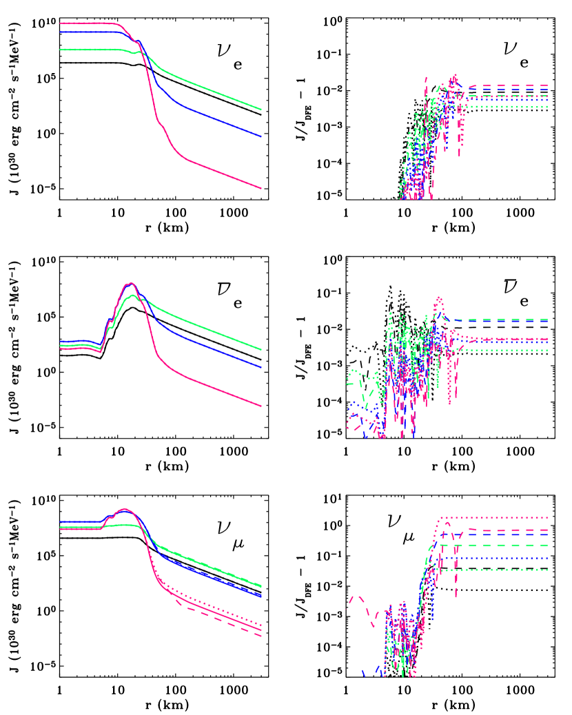
Figure 7.— A comparison of the three different formal solvers, namely the Discontinuous Finite Element (DFE) scheme, the first-order short characteristics (SC) scheme, and the Feautrier scheme. On the left-hand panels, the mean intensity $J$ is plotted as a function of radius for four selected energy groups, with $E=4.6$ MeV (black), 11.7 MeV (green), 40 MeV (blue), and 74 MeV (red). Full lines display the DFE results, dotted lines the SC results, and dashed lines the results obtained by the Feautrier scheme. The right-hand panels display the corresponding relative differences of the mean intensities with those computed by the DFE scheme, namely $J({\rm solver})/J({\rm DFE})-1$: dashed lines – Feautrier; dotted lines – SC.

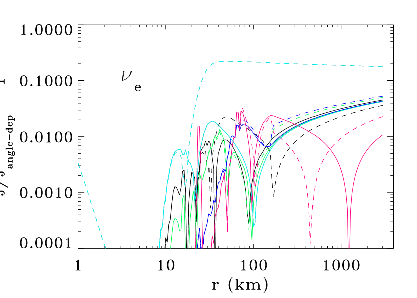
Figure 8.— A comparison of the relative differences of the mean intensity computed by the angle-dependent solver and by the moment equation solver, $J({\rm angle\ dep.\ solver})/J({\rm moment\ solver})-1$. The dashed lines represent the original solver, without the sphericity factors; solid lines the moment solver with sphericity factors. The color pattern is analogous to that used in Fig. 7; the only difference is an added energy group with $E=1$ MeV, represented by the light-blue [turquoise] lines.

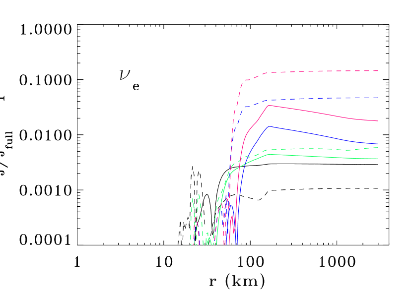
Figure 9.— A comparison of the relative differences of mean intensity for the full velocity-dependent, anisotropic scattering solution with that setting $\delta=0$ (that is, assuming isotropic scattering), but keeping the velocity-dependent terms (solid lines); and with setting $v=0$ (but keeping $\delta\not=0$ – dashed lines. The color pattern is the same as in Fig. 7.

Figure 10.— A comparison of the net heating rate (“gain”) for the full velocity-dependent, anisotropic scattering solution (full lines) with that setting $\delta=0$ (that is, assuming isotropic scattering), but keeping the velocity-dependent terms (dashed lines); and with setting $w=0$ (but keeping $\delta\not=0$) – dotted lines. Crosses (which lie indistinguishably close to the dotted line) represent the solution with both $w=0$ and $\delta=0$. Note that the sign of the $w$-correction to the net gain is different from that found in the comoving-frame formalism (Buras et al. 2006). See text for a discussion.

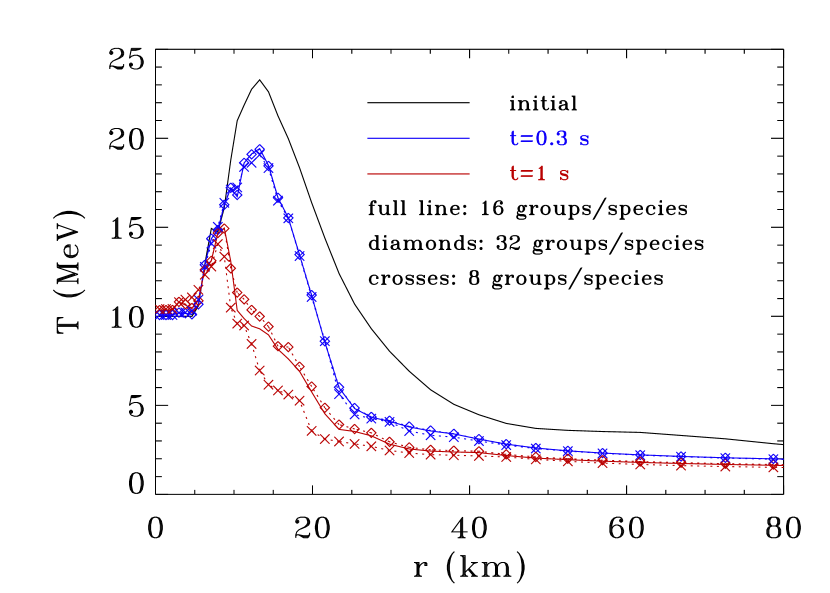
Figure 11.— Temperature as a function of radius, for the initial configuration (full black line), and for 0.3 seconds (blue lines/symbols) and 1 second (red lines and symbols) of evolution. Solid lines display the evolution where we employ 16 energy groups per neutrino species; diamonds display the evolution where we employ 32 energy groups per neutrino species, and crosses display models where we employ 8 energy groups per neutrino species.

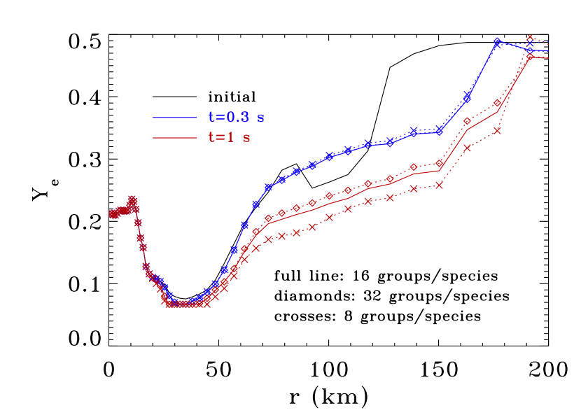
Figure 12.— The same as in Fig. 11, but for $Y_{e}$.

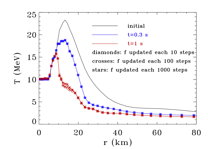
Figure 13.— Temperature as a function of radius, for the initial configuration (full black line), and for 0.3 seconds (blue lines/symbols) and 1 second (red lines and symbols) of evolution. Diamonds display the evolution where the Eddington factor ($f$) was updated every 10 timesteps; crosses display models where the Eddington factor was updated every 100 timesteps, while stars display models where the Eddington factor was updated every 1000 timesteps. Notice that in many instances all the symbols overlap.

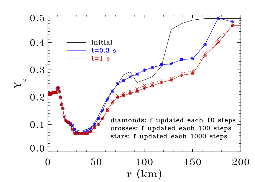
Figure 14.— The same as in Fig. 13, but for $Y_{e}$.

References

- Auer (1971) Auer, L.H., 1971, J. Quant. Spec. Radiat. Transf., 11, 573
- Auer (1991) Auer, L.H., 1991, in Stellar Atmospheres: Beyond Classical Models, ed. by L. Crivellari, I. Hubeny, and D.G. Hummer, NATO ASI Ser. C, Vol. 341, p.9
- Bowers & Wilson (1982) Bowers, R.L. & Wilson, J.R. 1982, ApJS, 50, 115
- Bruenn (1985) Bruenn, S.W. 1985, ApJS, 58, 771
- Buras et al. (2006) Buras, R., Rampp, M., Janka, H.-Th., & Kifonidis, K. 2006, A&A, 447, 1049
- Burrows, Hayes, & Fryxell (1995) Burrows, A., Hayes, J., & Fryxell, B.A. 1995, ApJ, 450, 830
- Burrows et al. (2006) Burrows, A., Livne, E., Dessart, L., Ott, C.D., & Murphy, J. 2006, ApJ, 640, 878
- Cardall & Mezzacappa (2003) Cardall, C.Y. & Mezzacappa, A. 2003, Phys. Rev. D, 68, 023006
- Cardall, Lentz, & Mezzacappa (2005) Cardall, C.Y., Lentz, E.J., & Mezzacappa, A. 2005, Phys. Rev. D, 72, 043007
- Castor, Dykema, & Klein (1992) Castor, J.I., Dykema, P.G., & Klein, R.I, 1992, ApJ, 387, 561
- (11) Dessart, L., Burrows, A., Ott, C.D., Livne, E., Yoon, S.-Y., & Langer, N. 2006a, ApJ, 644, 1063
- (12) Dessart, L., Burrows, A., Livne, E., & Ott, C.D. 2006b, astro-ph/0510229
- Hayes & Norman (2003) Hayes, J.C. & Norman, M.L. 2003, ApJ, 147, 197
- Herant et al. (1994) Herant, M., Benz, W., Hix, W.R., Fryer, C.L., & Colgate, S.A. 1994, ApJ, 435, 339
- Hubeny (2003) Hubeny, I., 2003, in ASP Conf. Ser. 288, Stellar Atmosphere Modeling, ed. I. Hubeny, D. Mihalas, and K. Werner, Astronomical Society of the Pacific, San Francisco, p.17
- Hubeny & Lanz (1992) Hubeny, I., & Lanz, T., 1992, A&A, 262, 501
- Hubeny & Lanz (1995) Hubeny, I., & Lanz, T., 1995, ApJ, 439, 875
- Klein et al. (1989) Klein, R.I, Castor, J.I., Dykema, P.G., Greenbaum, A., & Taylor, D., 1989, J. Quant. Spec. Radiat. Transf., 41, 199
- (19) Janka, H.-T., Buras, R., Kifonidis, K., Marek, A., & Rampp, M. 2005, in Cosmic Explosions, On the 10th Anniversary of SN1993J. Proceedings of IAU Colloquium 192, edited by J.M. Marcaide and Kurt W. Weiler, Springer Proceedings in Physics, vol. 99. (Berlin: Springer), p.253 (astro-ph/0401461)
- (20) Janka, H.-Th., Buras, R., Kitaura Joyanes, F.S., Marek, A., Rampp, M., & Scheck, L. 2005, “Neutrino-driven supernovae: An accretion instability in a nuclear physics controlled environment,” in Proceedings of the 8th International Symposium on Nuclei in the Cosmos, Vancouver, Canada, July 19–23, 2005, Nuclear Physics A, 758, 19–26
- Lanz & Hubeny (2003) Lanz, T., & Hubeny, I., 2003, ApJS, 146, 417
- LeBlanc & Wilson (1970) LeBlanc, J.M. & Wilson, J.R., 1970, ApJ, 161,541
- (23) Liebendörfer, M. et al. 2001a, Phys. Rev. D, 63, 103004
- (24) Liebendörfer, M., Mezzacappa, A., Thielemann, F.-K. 2001b, Phys. Rev. D, 63, 104003
- Liebendörfer et al. (2004) Liebendörfer, M., Messer, O.E.B., Mezzacappa, A., Cardall, C.Y., & Thielemann, F.-K. 2004, ApJS, 150, 263
- Liebendörfer et al. (2005) Liebendörfer, M., Rampp, M., Janka, H.-Th., & Mezzacappa, A. 2005, ApJ, 620, 840
- Livne et al. (2004) Livne, E., Burrows, A., Walder, R., Thompson, T.A., and Lichtenstadt, I. 2004, ApJ, 609, 277
- Mayle, Wilson, & Schramm (1987) Mayle, R., Wilson, J.R., & Schramm, D.N. 1987, ApJ, 318, 288
- Mezzacappa & Bruenn (1993) Mezzacappa, A. & Bruenn, S.W. 1993, ApJ, 410, 669
- Mezzacappa et al. (2001) Mezzacappa, A., Liebendörfer, M., Messer, O.E.B., Hix, W.R., Thielemann, F.-K., & Bruenn, S.W. 2001, Phys. Rev. Lett., 86, 1935
- Mihalas & Klein (1982) Mihalas, D. & Klein, R.I. 1982, Journal of Computational Physics, 46, 97
- Mihalas, Kunasz, & Hummer (1975) Mihalas, D., Kunasz, P.B., & Hummer, D.G., 1975, ApJ, 202, 465
- Mihalas & Mihalas (1984) Mihalas, D. & Mihalas, B., Foundations of Radiation Hydrodynamics, New York, Oxford University Press, 1984
- Ng (1974) Ng, K.C., 1974, J. Chem. Phys., 61, 2680
- (35) Ott, C.D., Burrows, A., Dessart, L., & Livne, E. 2006a, ApJ Suppl., 164, 130
- (36) Ott, C.D., Burrows, A., Dessart, L., & Livne, E. 2006b, Phys. Rev. Lett., 96, 201102
- Rampp & Janka (2000) Rampp, M. & Janka, H.-T. 2000, ApJ, 539, L33
- Rampp & Janka (2002) Rampp, M. & Janka, H.-Th. 2002, A&A, 396, 331
- Stone, Mihalas, & Norman (1992) Stone, J.M., Mihalas, D., & Norman, M.L. 1992, ApJS, 80, 819
- (40) Rybicki, G. & Hummer, D.G., 1991, A&A, 245, 171
- (41) Swesty, F.D., & Myra, E.S. 2005a, astro-ph/0506178
- (42) Swesty, F.D., & Myra, E.S. 2005b, astro-ph/0507294
- Swesty & Myra (2006) Swesty, F.D., & Myra, E.S. 2006, astro-ph/0607281
- Thompson, Burrows, & Pinto (2003) Thompson, T.A., Burrows, A., & Pinto, P.A. 2003, ApJ, 592, 434
- Wilson (1985) Wilson, J.R. 1985, in Numerical Astrophysics, ed. J. Centrella, J. M. LeBlanc, R. L. Bowers (Boston: Jones & Bartlett), p. 422
- Walder et al. (2005) Walder, R., Burrows, A., Ott, C.D., Livne, E., Lichtenstadt, I., & Jarrah, M. 2005, ApJ, 626, 317