Investigating the Andromeda Stream: III. A Young Shell System in M31

Abstract

Published maps of red giant stars in the halo region of M31 exhibit a giant stellar stream to the south of this galaxy, as well as a giant “shelf” to the northeast of M31’s center. Using these maps, we find that there is a fainter shelf of comparable size on the western side as well. By choosing appropriate structural and orbital parameters for an accreting dwarf satellite within the accurate M31 potential model of Geehan et al. (2006), we produce a very similar structure in an $N$-body simulation. In this scenario, the tidal stream produced at pericenter of the satellite’s orbit matches the observed southern stream, while the forward continuation of this tidal stream makes up two orbital loops, broadened into fan-like structures by successive pericentric passages; these loops correspond to the NE and W shelves. The tidal debris from the satellite also reproduces a previously-observed “stream” of counterrotating PNe and a related stream seen in red giant stars. The debris pattern in our simulation resembles the shell systems detected around many elliptical galaxies, though this is the first identification of a shell system in a spiral galaxy and the first in any galaxy close enough to allow measurements of stellar velocities and relative distances. We discuss the physics of these partial shells, highlighting the role played by spatial and velocity caustics in the observations. We show that kinematic surveys of the tidal debris will provide a sensitive measurement of M31’s halo potential, while quantifying the surface density of debris in the shelves will let us reconstruct the original mass and time of disruption of the progenitor satellite.

1 INTRODUCTION

Our neighboring disk galaxy M31 has turned out to be a well-equipped laboratory for research into the accretion and disruption of substructure in galactic halos. A stellar stream of length $\sim\!120\,\mbox{kpc}$ is observed to flow from its tip south and behind M31 into M31’s center (Ibata et al., 2001; McConnachie et al., 2003; Ibata et al., 2004; Guhathakurta et al., 2006), while many other irregular morphological and kinematic features indicative of accretion are seen in the galactic disk and halo (Ferguson et al., 2002; Merrett et al., 2003; Ibata et al., 2005). The giant southern stream is thought to be formed at the last pericentric passage of a progenitor satellite with mass $\sim\!10^{9}\,M_{\sun}$ on a highly radial orbit (Ibata et al., 2004; Font et al., 2006; Geehan et al., 2006, hereafter Paper I; Fardal et al., 2006, hereafter Paper II). This stream holds out the promise of the first precise measurements of the gravitational potential in M31’s halo. This is important for many reasons, including breaking the disk-halo degeneracy in the mass distribution (Paper I) and thereby understanding the response of the dark halo to the central baryons. However, there are two obstacles to these measurements at present (Paper II). First, the current observational errors on the distance allow too much flexibility in the orbits to constrain the potential effectively. Second, the stream does not follow a single orbit, but has a gradient of energy along the length of the stream, “tilting” the stream in phase space relative to the orbit and biasing the measurement of the potential. The amount of this tilt depends on the location of the progenitor, which is currently unknown. Locating the progenitor would both specify the stream-orbit tilt and constrain the allowed orbital trajectories, removing both obstacles.

The “Northeast Shelf”, a faint diffuse feature seen to the NE side of M31 in the red giant branch (RGB) star-count maps of Ferguson et al. (2002), has been suggested as a possibility for the current location of the progenitor, or at least as the forward continuation of the stream (Ibata et al., 2004; Font et al., 2006). Below we find that there is a similar, even fainter shelf or plateau on the other side of M31, which we call the “Western shelf”. In this paper, we focus on the possibility that the forward continuation of the stream makes up these NE and W shelves. In this scenario, the shelves are a similar phenomenon to the “shell” systems seen around many elliptical galaxies. These systems are believed to be produced by tidal disruption of a satellite galaxy on a nearly radial orbit (e.g., Schweizer, 1980; Quinn, 1984; Hernquist & Quinn, 1988; Barnes & Hernquist, 1992), exactly the phenomenon believed to be responsible for the creation of M31’s southern stream, so it is not unexpected that shell-like features should be present. These coherent structures are rich in information. For example, they allow sensitive tests of the potential of the host galaxy without the need for distance information (Merrifield & Kuijken, 1998), if the necessary kinematic observations can be obtained as is possible for the first time in the M31 shells. Also, there exists a simple relation between the surface density of a shell and the rate at which stellar mass flows through the shell; when appied to the W shelf, this can be used to deduce the orbital parameters and the mass of the satellite that produced the observed debris.

Our purpose in this paper is threefold: first, to show that this paradigm of a shell debris pattern is consistent with the current observations of M31; second, to explain the basic physics that gives rise to the spatial and kinematic pattern of the debris; and third, to find observational diagnostics to further constrain the model of the debris from present and future datasets. In § 2, we give an overview of the complex observed structure around M31, and describe our scenario to explain a major part of this structure. In § 3, we explain our methods for setting up and running a simulation of this scenario. We then compare the simulation results to the observed properties of the debris around M31, to see whether our model is plausible. In § 4, we discuss the physics that governs this model of the satellite debris. We consider several observables that can be used to confirm or rule out our scenario, and to constrain the physical properties of the stream and its progenitor. In § 5, we discuss some remaining issues regarding our model, and state our conclusions.

2 SCENARIO OF SHELF FORMATION

Figure 1a shows the density of RGB stars around M31 (from Irwin et al., 2005). The sky coordinates $\xi$ and $\eta$ in the eastern and northern (E and N) directions respectively are “standard coordinates” centered on M31. Several features that will be important in the discussion below are marked, including the southern (S) stream. The overdensity known as the NE shelf (Ferguson et al., 2002; Ferguson et al., 2005) is also readily apparent.

Less obviously, there is a similar enhancement of lower surface brightness on the W side, which is apparent on close visual inspection in this map and several of its earlier incarnations (Ferguson et al., 2002; Lewis et al., 2004; McConnachie et al., 2004; Ferguson et al., 2005). To enhance this structure, we display in Figure 1b a map obtained from Figure 1a using the Sobel edge-detection operator, which turns sharp edges into bright ridges. We fit the NE and W shelf ridges in this map with smooth curves, whose interpolating points are given in Table 1. The fainter W shelf has not previously been been singled out as an interesting feature in the literature, but it appears clearly enough here to investigate its possible origins.

Several other interesting features show up in Figure 1b, among them the “Northern Spur”, a bright loop at $\xi\approx 0.8^{\circ}$, $\eta\approx 1.8^{\circ}$; the “G1 clump” and related structure near the SW major axis at the outer regions of the disk; and a shelf in the southern stream at $\eta\approx-1.0^{\circ}$. Whether these other features have any relation to the stream itself is not currently known.

Figure 1: Panel a: Map of RGB count density, from Irwin et al. (2005). The edges of the NE and W shelves that are the focus of this paper are marked with red dotted lines. The H13d field of Reitzel et al. (2006) and four fields from Ibata et al. (2005) discussed below are marked with crosses. Panel b: Sobel-filtered version of Panel a, which detects sharp edges in the count map. To create this map, we fill in sharp features such as plot annotations and noise spikes with the surrounding pixel values, smooth the map, and apply the Sobel operator. We then fit a smooth curve to the shelf edges, which again are shown by dotted lines.

Table 1: Position of shelf edges (dotted lines in Figure 1).

$\xi$ (∘)	$\eta$ (∘)	$R_{proj}$ (∘)
NE shelf
1.95	1.46	2.43
1.96	0.93	2.17
1.91	0.59	2.00
1.86	0.41	1.91
1.78	0.31	1.81
1.70	0.17	1.71
1.45	$-0.01$	1.45
W shelf
$-0.56$	1.61	1.70
$-1.03$	1.49	1.81
$-1.45$	1.16	1.85
$-1.58$	0.97	1.86
$-1.78$	0.47	1.84
$-1.87$	0.17	1.87
$-1.92$	$-0.31$	1.94
$-1.95$	$-0.56$	2.03

In Paper II, we found that the southern stream is well explained by a baryon-dominated dwarf satellite of mass $\sim\!10^{9}\,M_{\sun}$, experiencing its first pass through M31 pericenter. Generically, in such a collision, much of the satellite’s mass is stripped and turns into leading and trailing tidal streams. These two streams are roughly symmetric about the progenitor, though the leading stream spirals in towards the primary galaxy and the trailing stream outwards from it, as one traces the streams away from the progenitor. In M31, the trailing, higher-energy stream is the one that must correspond to the observed southern stream, since the surface density is observed to fall off towards the tip of this stream opposite to its direction of motion. The locations of the progenitor itself and of the forward, lower-energy stream are currently unknown. If the satellite should still be intact at its next pericentric passage, it again produces two streams, which nearly overlay the portions of the original stream nearest the satellite. A clear example of such a multiple stream system is shown in Law, Johnston, & Majewski (2005) using a simulation of the Sagittarius galaxy.

Since the progenitor is not observed along M31’s southern stream, which spans a range of $\sim\!0.4$ in orbital phase (measured in units of the radial period), it is likely that the stream continues at least an equal amount of 0.4 periods ahead, taking it past the next pericenter (the second in our numbering scheme) and at least a significant part of the way to the next apocenter. In Paper II, we could not trace the continuation of the southern stream precisely past the second pericenter where it merges into M31’s bulge and disk. However, we found that it was constrained to lie on the NE side of M31. We found an acceptable (if not optimal) orbital fit putting the progenitor in the area of the NE shelf. In contrast, the progenitor would need one more pericentric passage (its third) to reach the W shelf, as would any material in the tidal stream. We also see in Figure 1 that the surface density of the W shelf is lower than for the NE shelf, as if the density were tailing off in the stream forward of the progenitor.

These facts lead us to our basic scenario: as we follow the continuation of the southern stream further forward in the orbital trajectory, the debris first produces a diffuse shelf on the E side of M31, and subsequently a similar shelf on the W side. Depending on the current position and state of the progenitor, the NE shelf may be made up solely of material from the forward continuation of the S stream, or include the remnant of the progenitor and the streams created at its second pericentric passage as well. In the next section, we test this scenario.

3 SIMULATION OF DEBRIS PATTERN VERSUS OBSERVATIONS

3.1 Method

In Papers I and II, we discussed the physical geometry of M31 and its surrounding system of satellites and streams. We then derived a bulge-disk-halo model for M31’s gravitational potential (Paper I), and developed a method for fitting the orbit of the stream’s progenitor given the observed properties of the stream (Paper II). It is worth repeating here M31’s heliocentric radial velocity of $-300\,\mbox{km}\,\mbox{s}^{-1}$ (de Vaucouleurs et al., 1991). Also, we assume the distance to M31 is $z_{g}=784\pm 24\,\mbox{kpc}$ (Stanek & Garnavich, 1998), which agrees very well with the distance of $z_{g}=785\pm 25\,\mbox{kpc}$ derived from the RGB maps by McConnachie et al. (2005), and implies that $1^{\circ}$ in angle corresponds to $13.5\,\mbox{kpc}$.

To construct a model of the progenitor, we first estimate its orbit, using the methods similar to those in Paper II. For the NE shelf we assume a central position on the sky of $\xi=1.8^{\circ}$, $\eta=0.7^{\circ}$. We fit a progenitor trajectory to pass in the direction (not necessarily the exact location) of this point, while still reproducing the observational properties of the southern stream, obtained by analytically “stretching” the trajectory to approximate the phase-space location of the stream ((see Paper II, for details)). We also incorporate the radii and velocities of the Merrett et al. (2006) northeastern “Stream” PNe into the fit, constraining the orbit to pass near their projected radii and line-of-sight velocities.

The M31 potential model here is a member of the family of models described in Paper I, and includes a Hernquist (1990) bulge, an exponential disk, and a Navarro, Frenk, & White (1996, henceforth NFW) halo. The specific parameters used here imply a low-mass disk. The results are not strongly sensitive to the disk mass, though, since the rotation curve places strong constraints on the overall potential.

Table 2: Simulation Parameters

Parameter	Symbol	Value	Comments
Satellite structure
Progenitor Mass	$M_{s}$	$2.2\times 10^{9}\,M_{\sun}$	Plummer Sphere
Progenitor Radius	$a_{s}$	$1.03\,\mbox{kpc}$
Central Surface Density	$\Sigma_{0,s}$	$6.57\times 10^{8}\,M_{\sun}\,\mbox{kpc}^{-2}$
Central Velocity Dispersion	$\sigma_{0,s}$	$39.1\,\mbox{km}\,\mbox{s}^{-1}$	1-dimensional
Particle Mass	$m_{p}$	$1.68\times 10^{4}\,M_{\sun}$
Particle Number	$N_{p}$	131072
Satellite orbit
Initial position∗	$x_{0}$	$-34.75\,\mbox{kpc}$
	$y_{0}$	$19.37\,\mbox{kpc}$
	$z_{0}$	$-13.99\,\mbox{kpc}$
Initial velocity∗	$v_{x0}$	$67.34\,\mbox{km}\,\mbox{s}^{-1}$
	$v_{y0}$	$-26.12\,\mbox{km}\,\mbox{s}^{-1}$
	$v_{z0}$	$13.50\,\mbox{km}\,\mbox{s}^{-1}$
Final time	$t_{0}$	$840\,\mbox{Myr}$
M31 structure
Total Bulge Mass	$M_{b}$	$3.24\times 10^{10}\,M_{\sun}$	Hernquist Sphere
Total Disk Mass	$M_{d}$	$3.66\times 10^{10}\,M_{\sun}$	Exponential Disk
Total Mass inside 125 kpc	$M(<125\;{\rm kpc})$	$7.3\times 10^{11}\,M_{\sun}$
Virial Mass	$M_{200}^{\ast}$	$8.8\times 10^{11}\,M_{\sun}$
	$M_{100}^{\ast}$	$9.5\times 10^{11}\,M_{\sun}$
Bulge Scale Radius	$R_{b}$	$0.61\,\mbox{kpc}$
Disk Scale Radius	$R_{d}$	$5.40\,\mbox{kpc}$
Disk Scale Height	$z_{d}$	$0.60\,\mbox{kpc}$
Halo Scale Radius	$r_{h}$	$7.63\,\mbox{kpc}$
NFW profile Virial Radius	$R_{200}^{\dagger}$	$195\,\mbox{kpc}$
	$R_{100}^{\dagger}$	$253\,\mbox{kpc}$
Disk Central Surface Density	$\Sigma_{0}$	$2.0\times 10^{8}\,M_{\sun}\,\mbox{kpc}^{-2}$
Halo Density Parameter	$\delta_{c}$	$4.41\times 10^{5}$	characteristic density relative to critical
Halo Concentration Parameter	$C_{200}\equiv R_{200}/r_{h}$	25.5
Maximum Rotation Velocity	$V_{c,max}$	$259\,\mbox{km}\,\mbox{s}^{-1}$
∗ $x$, $y$, and $z$ here are coordinates in a system where $x$ points to the E and $y$ to the N in the plane of the sky, and $z$ points into the sky.
† $M_{\Delta}$ is the mass enclosed within radius $R_{\Delta}$ such that the mean density inside is $\Delta\rho_{c}$, where $\Delta=100$ or $200$ (see Paper I).

Our approximate analytic method describes only the central path of the debris in phase space. To gain a more complete picture of the debris pattern, we turn to $N$-body simulations. We continue to use a fixed potential to represent the influence of M31, but the progenitor is now represented by self-gravitating particles. We consider a purely stellar system. It is hard to put much dark matter in the progenitor without either underproducing the amount of stellar mass seen in the stream, or overproducing its observed width and velocity dispersion (Paper II). The progenitor is given a spherical Plummer-law density profile, with rough values of the initial mass and scale radius $M_{s}\sim 10^{9}\,M_{\sun}$ and $a_{s}\sim 1\,\mbox{kpc}$ (later to be refined). We initialize the particles of this hot spherical system with the ZENO package of J. Barnes. The particle velocities are assumed to be isotropic, and are set by solving an Abel integral for the energy distribution rather than assuming a Maxwellian (see Binney & Tremaine, 1987), giving an initial configuration very close to equilibrium.

Using the orbit from the fit above, the satellite is set in motion inbound and slightly past apocenter, minimizing initial transients from M31’s tidal forces. The formation of the progenitor and its accretion into M31’s halo are not modeled here. Once we determine the current state of the debris, we should be able to shed some light on the progenitor’s prior history, but for now it lies outside the scope of our work.

We run the simulations with the multistepping tree code PKDGRAV (Stadel, 2001). We set the spline softening length to a small fraction of the satellite’s Plummer scale radius, $\epsilon=0.1a_{s}\sim 100\,\mbox{pc}$. The gravity tree uses an opening angle $\theta=0.8$, the node forces are expanded to hexadecapole order, and the individual particle timesteps $\Delta t_{i}$ are related to the particle acceleration $a_{i}$ by the criterion $\Delta t_{i}<\eta(\epsilon/a_{i})^{1/2}$ with $\eta=0.2$.

We ignore the effect of dynamical friction in both our orbital fitting procedure and in the $N$-body simulations. This is reasonable given that we are not aiming at an exact fit of the observations, since the mass of the progenitor satellite is small relative to the total mass of M31 ($\sim\!10^{-2}$), and since the Coulomb logarithm is small as well ($\ln\Lambda\sim 3$). Even so, the specific orbital energy of the progenitor decreases somewhat during the run, since the energy required to tidally disrupt and heat the satellite comes at the expense of the satellite’s orbital energy. We ignore any perturbations from M32 or NGC 205 as well. Their mass is low enough that a significant deflection would require an unlikely close passage, and their orbital parameters are not known well enough for us to treat this possibility with any reliability.

To relate the numerical simulations to observable properties of the stream, we assume a fixed $M/L$ ratio throughout the stellar population, or more precisely a fixed ratio of stellar mass to RGB star numbers, since it is the latter class of objects that are used to trace the observed stream and related debris. We also assume a fixed ratio of stellar mass to PNe number. Merrett et al. (2006) showed that there is good agreement between the number counts of PNe and M31’s $r$-band light profile, which traces the old stars and thus the stellar mass quite well.

Our initial orbital fit yielded promising results. We then ran several more simulations to choose the mass and size of the satellite, essentially through trial and error, to match the length of the southern stream and other observable features. We also attempted to optimize the orbital parameters further using $N$-body simulations, but without clear further improvement. The parameters of our final simulation are given in Table 2. We note that we have certainly not explored our large parameter space carefully in this search. Also, it is not yet possible to make quantitative comparison to some of the most relevant observational data such as the RGB spatial distribution, due to thorny issues such as incompleteness and contamination from both foreground Milky Way dwarf stars and background galaxies. Hence, we make no claims that our present satellite orbital parameters are optimal. They should, however, suffice to demonstrate the basic physical and observational properties we can plausibly expect from this general scenario.

Our spherical Plummer model for the satellite with initial mass $M_{s}=2.2\times 10^{9}\,M_{\sun}$ and scale radius $a_{s}=1.03\,\mbox{kpc}$ produces a central velocity dispersion of $39\,\mbox{km}\,\mbox{s}^{-1}$, consistent with typical velocity dispersions for galaxies of this mass (Dekel & Woo, 2003). The observed stream stars appear to have a moderately high metallicity, [Fe/H] $\approx-0.5$ (McConnachie et al., 2003; Guhathakurta et al., 2006; Kalirai et al., 2006b), and intermediate to old ages of 4–$11\,\mbox{Gyr}$ (Brown et al., 2006a, b). Again comparing to Dekel & Woo (2003), this observed metallicity is in very good agreement with the assumed progenitor mass. If we assume a $V$-band $M/L$ ratio of 5 in the progenitor, appropriate for a baryon-dominated galaxy with an old stellar population and a Salpeter initial mass function, the central surface brightness is $\Sigma_{0}\approx 1.3\times 10^{8}\,L_{\sun,V}\,\mbox{kpc}^{-2}$. This is a factor of 3 below the mean regression line of Dekel & Woo, but is still consistent with the scatter about this line. The Plummer law is not particularly concentrated towards the center. If we had adopted an $R^{1/4}$ law for the satellite, the central surface brightness would have been about 300 times larger, for the same total luminosity and projected half-mass radius.

We run the satellite model with PKDGRAV for 2 Gyr. The first pericentric passage occurs at 0.17 Gyr, giving rise to the southern stream. The first apocenter occurs at 0.44 Gyr and the second pericenter at 0.70 Gyr. We select the output that most closely resembles the spatial and kinematic properties of the stream and shelf debris. This output occurs at 0.84 Gyr past the start of the simulation (Table 2). At this point the progenitor has been completely disrupted and its central stars lie in the location of the observed NE shelf. We first tried runs with a small number of particles before proceeding to the final run; we did not find any significant differences resulting from particle resolution.

In several of the plots below, we will use only the simulated satellite particles for clarity of presentation. However, when comparing to the observations, it is essential to have an idea of the characteristics of the main stellar body of M31, which in projection is coincident with much of the satellite debris. Both Ferguson et al. (2005) and Brown et al. (2006a) found that at 10–20 kpc from M31’s center, the stellar populations of the spheroid and of the stream were quite similar. On the other hand, an outer halo component has recently been discovered in M31 (Guhathakurta et al., 2005; Irwin et al., 2005; Kalirai et al., 2006a; Chapman et al., 2006); incorporating these new observations, the mean metallicity of the smooth M31 spheroid is seen to decreases radially outward down to [Fe/H] $\approx-1.4$ at $R\ga 60\,\mbox{kpc}$. In contrast, the stream’s mean metallicity is more or less constant along its length, out to similar projected radii. So depending on location, the characteristics of the stellar population may or may not be useful for separating the contributions of the stream debris and M31; in some regions kinematics may be the only guide.

Therefore, we construct an $N$-body particle realization of M31 itself to mimic the observed stellar components of M31, and combine it with the satellite debris to predict the full spatial and velocity pattern. We only add this particle realization at the end, rather than evolving it dynamically with the $N$-body code. The model in Paper I predated the discovery of the metal-poor halo component just mentioned; it is important to include this in the model to estimate the M31 contribution at large radii. We model the halo stars by assuming that a small fraction of the NFW halo mass is composed of stars rather than dark matter, equivalent to using an NFW profile normalization $\delta_{c,\ast}=350$. To fit the profile better, we also truncate the Hernquist bulge past $r_{tr,b}=10\,\mbox{kpc}$ since it would otherwise overproduce the surface brightness near 20 kpc. We use the default truncation scheme in ZENO, which cuts off $dM(r)/dr$ as an exponential past the truncation radius. (We neglect this truncation in the orbit calculation, since it changes the mass within 125 kpc by only 0.2%.) With these modifications, the composite stellar profile exhibits a change in slope at $\sim\!30\,\mbox{kpc}$ similar to that in the observed profile (Guhathakurta et al., 2005; Irwin et al., 2005; Kalirai et al., 2006a).

For our $N$-body realization of M31, we use the same particle mass as for the progenitor particles, and again use the same constant scaling of RGB or PNe number to stellar mass. Given that there are slight but observable stellar population differences between M31’s giant stream and spheroid (Ferguson et al., 2005; Brown et al., 2006a; Kalirai et al., 2006b, a; Brown et al., 2006b), our constant scaling assumption is a slight oversimplification. Moreover, there are significant observed deviations from our simple model in the form of spiral arms, warping of the disk, and elongation of the bulge and inner disk. Our model should thus be taken as an illustrative proxy for the M31 stellar component, rather than a precise description.

3.2 Shelf morphology

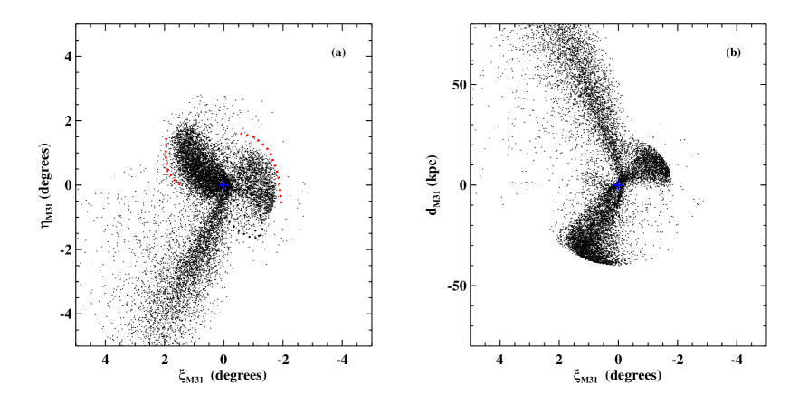
Figure 2: The spatial distribution of satellite debris particles in the simulation, centered on M31. Panel a: sky projection in standard coordinates. This can be compared to the observed star-count map in Figure 1a. The red dotted lines show the observed shelf edges from that figure. For clarity, a randomly chosen subset of particles is shown in this and most subsequent figures. The particles of our static M31 model are also omitted; the disk component of that model would dominate much of the NE shelf but only a small portion of the W shelf. Panel b: the view of the debris looking down the north axis in Panel (a). “Depth” $d_{M31}$ increases with distance from Earth. The scale on that axis matches the angular scale at M31’s mean distance of $\approx 780$ kpc. The NE shelf is directed mainly toward us, while the W shelf is oriented away from us close to the plane of the sky.

We begin the comparison to observations by examining the pattern on the sky of the NE and W shelves. The spatial distribution of the particles in our simulation is shown in Figure 2. The debris resembles the observed shelves (shown in Figure 1) on both the E and W sides, with a much larger surface density on the E side. The edges of these shelves are at similar, but in some places slightly smaller radii to the observed edges. The shelves also cover about the right azimuthal range, though the faintness of the features and interference from M31 itself make it difficult to make a precise comparison

We note that the projected radius of the NE shelf from M31’s center, as shown in Figure 1 and given in Table 1, appears to vary with azimuth, instead of forming a circular arc. This may be a significant clue to the nature of the shelf. In contrast, the edge of the W shelf appears more circular. The simulations appear to reproduce the behavior of projected radius as a function of azimuth for both shelves.

We next turn to the surface densities. In the star-count map of Irwin et al. (2005), the brightness of the NE shelf appears similar to the denser, innermost distinct parts of the S stream (at $R_{proj}\approx 1.6^{\circ}$), while the brightness of the W shelf appears more similar to the more tenuous middle parts of the S stream (at $R_{proj}\approx 2.5^{\circ}$). To obtain a crude estimate of the surface densities in the latter regions, we first construct a simple estimate for the southern stream surface brightness using the transverse and longitudinal profiles in McConnachie et al. (2003). We normalize these profiles by using the stream’s $V$ magnitude of $M_{V}=-14.0$ or $V$ luminosity of $3.4\times 10^{7}L_{\sun,V}$ in the range $15\,\mbox{kpc}\la R_{proj}\la 40\,\mbox{kpc}$ from M31’s center (Ibata et al., 2001). Assuming a stellar $M/L_{V}\approx 5$ as before, this gives a stream stellar mass within this radial range of $\sim 2\times 10^{8}\,M_{\sun}$. Computing the surface density of the resulting mass model in the areas mentioned above, we can then estimate that the NE and W shelf surface densities are very roughly $\sim\!1.0\times 10^{6}\,M_{\sun}\,\mbox{kpc}^{-2}$ and $\sim\!8\times 10^{5}\,M_{\sun}\,\mbox{kpc}^{-2}$ respectively. We arbitrarily define the inner radial boundary of both shelves to be 60% of their outer radii (listed in Table 1) in order to isolate the regions in which the shelves have the highest contrast against the smooth M31 components; the NE shelf has an area $150\,\mbox{kpc}^{2}$ and the W shelf has an area $200\,\mbox{kpc}^{2}$. This then implies masses of $\sim\!1.5\times 10^{8}\,M_{\sun}$ within both shelf boundaries. We have not attempted here to subtract the background density of M31 disk and spheroid stars, so these surface densities and masses are only lower limits. Also, these estimates only apply to the mass inside our assigned boundary; if the shelf mass distribution continues radially inwards onto the face of M31, the total mass could be much larger. Given all the uncertainties, these are clearly only order-of-magnitude estimates, but even so should be good enough to check the plausibility of the model.

We compute the mass of the satellite debris particles in the simulation that lie within the boundaries of the NE and W shelf regions as defined above, and find $1.2\times 10^{8}\,M_{\sun}$ for the NE shelf and $1.4\times 10^{8}\,M_{\sun}$ for the W shelf (although these regions clearly do not select all the mass in the NE and W radial lobes). These imply surface stellar mass densities of $8\times 10^{5}\,M_{\sun}\,\mbox{kpc}^{-2}$ for the NE shelf and $7\times 10^{5}\,M_{\sun}\,\mbox{kpc}^{-2}$ for the W shelf. The former surface density in particular is a slight underestimate because it does not extend all the way to the observed shelf edge. Inclusion of the particles in the static M31 model raises these surface densities to $1.1\times 10^{6}\,M_{\sun}\,\mbox{kpc}^{-2}$ for the NE shelf and $1.0\times 10^{6}\,M_{\sun}\,\mbox{kpc}^{-2}$ for the W shelf. Comparison of these values with the rough observational estimates above shows that our model has passed another test.

M31 is close enough that the distribution in three spatial dimensions is measurable. Ferguson et al. (2005) used color-magnitude diagrams with HST/ACS to measure the brightness of red clump stars in the stream, 21 kpc in projection from the center of M31, and in the NE shelf, at $\xi=1.26^{\circ}$, $\eta=0.24^{\circ}$. They found that stars in the “NE shelf” fields indeed lay closer to us than those in the “Giant Stream” fields, by a factor $1.07\pm 0.01$. With the “depth” $d$ (defined here as the distance behind M31) in the stream field estimated to be $(50\pm 20)\,\mbox{kpc}$ by interpolating the results of McConnachie et al. (2003), this would put the shelf at depth $d_{\rm F05}=(0\pm 20)\,\mbox{kpc}$. However, Brown et al. (2006a) measured the red clump brightnesses at a nearly identical point in the stream and in a minor-axis, spheroid-dominated field, and found the stream there was only $(11\pm 5)\,\mbox{kpc}$ further than the spheroid position, which is likely at $d\approx 0$. From this estimate we can infer the shelf is at $d\approx-40\,\mbox{kpc}$, in front of M31.

Our model implies the material forming the NE shelf lies on average well in front of the center of M31, and hence even farther in front of the southern stream (see Figure 2). In the field of Ferguson et al. (2005), the median depth of the simulation particles is $d_{\rm F05}=-31\,\mbox{kpc}$, in agreement with the estimate based on Brown et al. (2006a), though the distribution is highly skewed with a small second peak at $\approx-5\,\mbox{kpc}$. The model thus appears to pass the test of the observed distances as well.

3.3 Velocity measurements

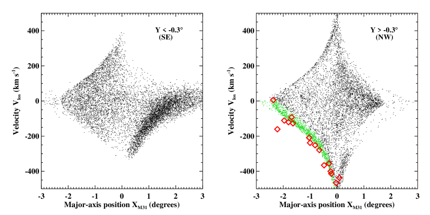
Figure 3: Plots of the velocities of satellite debris particles relative to M31 versus major axis position $X$, split on the basis of minor-axis position $Y$ into two panels. $X$ increases toward the SW, and $Y$ toward the NW. Left panel: southeast portion ($Y<-0.3^{\circ}$). The dense concentration of points at the lower right edge is the southern stream. Right panel: central and northwest portion ($Y>-0.3^{\circ}$). The PNe in M31 notated by Merrett et al. (2006) as “Stream” or “Stream?” are marked by red diamonds. The dense concentration of $N$-body particles within $60\,\mbox{km}\,\mbox{s}^{-1}$ of the lower left edge are marked in green; we regard these particles as an analogue to the Merrett et al. “PNe stream”.

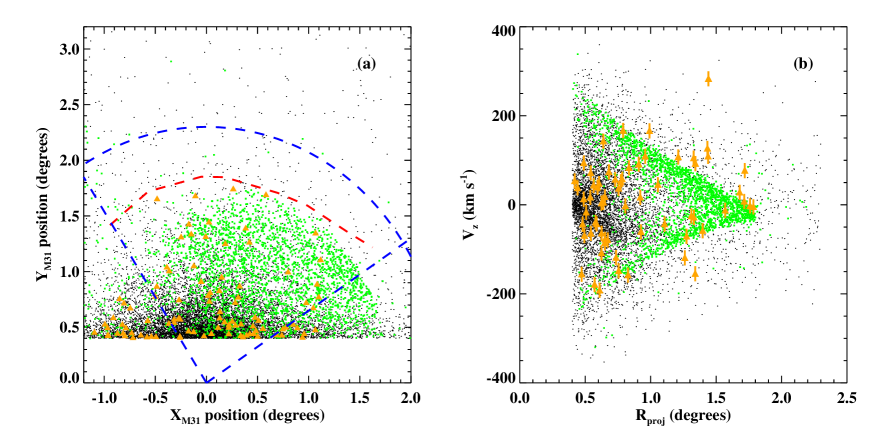
Figure 4: Plots of $N$-body particles and observed PNe in the W shelf region. Objects with minor axis coordinate $Y<+0.25^{\circ}$ are omitted. Panel a: sky position in M31-axis coordinates $X$ and $Y$. Green points show satellite debris particles, while black points show particles from the model of M31 itself. Orange triangles show observed PNe from Merrett et al. (2006), excluding those noted there as associated with NGC 205. The red dashed line shows the observed W shelf boundary from Figure 1 and Table 1. The sky coverage in the PNe survey extends roughly out to the outer blue dashed arc. Only objects shown within the blue dashed lines are selected for the next panel. Panel b: projected radius versus line-of-sight velocity. The symbols are the same as before. The PNe velocities have a measurement error of $17\,\mbox{km}\,\mbox{s}^{-1}$. Note the group of PNe close to the positions and velocities of the simulated shelf particles; this association is tested statistically in the text.

The overall velocity pattern in our simulation is shown in Figure 3. We will discuss the physical origin of the features in this plot later, in § 4.3. Here we only wish to compare the simulated velocities to the observed ones to see if they agree in their main respects. At present, there are three large-scale surveys that can constrain the overall velocity pattern of the observed debris: the wide-area survey of PNe by Merrett et al. (2003, 2006) and two ongoing surveys of RGB velocities in selected widely spaced fields (Ibata et al., 2004; Ibata et al., 2005; Chapman et al., 2006; Guhathakurta et al., 2006; Kalirai et al., 2006b, a; Gilbert et al., 2006).

The PNe detected by Merrett et al. include a component that moves opposite to the disk rotation on the NE side, with a narrow velocity width, suggestive of a continuation of the southern stream. The PNe indicated by Merrett et al. as “Stream” or “Stream?” are shown as triangles in the right panel of Figure 3. This apparent stream is unlikely to be produced by the usual stellar components of M31, so it is strongly indicative of some kind of tidal debris. The simulation produces a similar “stream” of material, due to a set of stars in the N part of the NE shelf which have similar velocities; like the observed PNe stream, these overlap the major axis of M31, as shown in Figure 9 below.

The Merrett et al. survey extends into an irregular area in the halo region of M31. In this region, Merrett et al. used wide-field images to optimize the choice of fields for closer study. These fields are sparse, so the survey coverage may change with position; we will ignore this potential complication. Figure 4a shows the survey results in the area of the W shelf; the survey coverage within the W shelf boundary (dashed red line) and between the dashed blue radial lines is almost complete, while it is sparser but not zero outside the W shelf boundary. We exclude the PNe that Merrett et al. find to be associated with NGC 205 on the basis of their positions and velocities. The same plot shows the simulation particles, including both the satellite debris (in green) and the particles from the static M31 model (in black). Although the number of PNe is limited, it seems that the density of PNe does not fall off all the way towards the W shelf; beyond $R\sim 0.7^{\circ}$ it remains roughly constant, suggesting that the PNe also trace the shelf. We plot the velocities of the PNe and simulation particles within the dashed selection boundary in Figure 4b. The satellite debris in the simulation forms a triangular shape in this plot. Interestingly, the PNe at large $R_{proj}$ mostly fall near the boundary of the simulated satellite debris; it appears that increasing the shelf radius or particle velocities slightly in the simulation would result in even better agreement.

To test this apparent agreement quantitatively, we compare two hypotheses: that the distribution matches the pure M31 particle distribution, or that it matches the sum of the M31 and satellite particles. We bin the particles in a grid covering the relevant area in projected radius and velocity, after convolving their velocities with a Gaussian distribution of $17\,\mbox{km}\,\mbox{s}^{-1}$, which is the random error in the PNe velocities. We then normalize the distributions, both including and excluding the satellite debris particles, to unity. The product of these binned distributions at the locations of the PNe then gives the likelihood function of these two hypotheses. We find that the likelihood ratio is about 180, meaning that the model with satellite debris is 180 times more likely than the model that excludes it, assuming equal prior probabilities. Furthermore, if as suggested by Figure 4, we add $30\,\mbox{km}\,\mbox{s}^{-1}$ to the velocities of the satellite particles as might be induced by a change to the overall angular momentum, the likelihood ratio increases to 4500. Thus these tests appear to show that some of these PNe are bona-fide members of the W shelf, and confirm its overall kinematic structure.

The remaining M31 radial velocity surveys use RGB stars. Previous analyses of substructure in these surveys mostly focus on the giant southern stream, the extended disk-like component (Ibata et al., 2004; Ibata et al., 2005; Guhathakurta et al., 2006), and the loop-like features near NGC 205 (McConnachie et al., 2004), but there are some hints of other structures. The stream of “counterrotating” PNe may have a counterpart in the inner disk RGB velocity measurements of Ibata et al. (2005, their Figure 9), though this feature is not discussed in that paper. Chapman et al. (2006) mention kinematic substructure in the NE that they attribute to a continuation of the southern stream, but the exact location of the responsible fields is not clear.

The RGB surveys obtain a much higher density of target objects than the PNe survey, albeit with a much sparser spatial coverage. Thus it is worth plotting the velocity distribution in each field as a separate histogram. We begin with the field H13d of Kalirai et al. (2006b) and Reitzel et al. (2006). The observational and simulation results are shown in Figure 5a. We include three curves that show the results of the simulation for the satellite debris alone, for the M31 model stars alone, and for the combination of the two. Here we assume the total mass density in the observations matches the total found in our simulation, and normalize the observational histogram accordingly. This method allows us to avoid the complex issues of the selection and detection efficiencies in the spectroscopic survey.

A substantial population at negative velocities, opposite to the sense of disk rotation, is evident in the observational histogram. This component is not visible at all in the galaxy model, but it matches the velocity distribution of the satellite debris quite well, even if the overall normalization is somewhat off. Another interesting feature is the difference in mean velocity, velocity dispersion, and possibly total mass between the observed and predicted disk components; we will return to this point below.

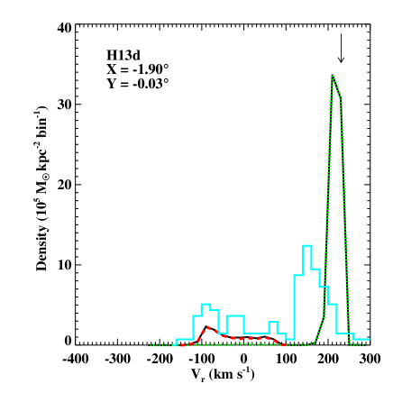
Figure 5: The velocity distribution relative to M31 in the field H13d of Reitzel et al. (2006) (also discussed in Kalirai et al., 2006b). The field used to select the simulation particles is taken to be a square $0.3^{\circ}$ on a side, to ensure a large sample of particles. Simulation results using the satellite debris alone are shown by a red dashed line; results using the M31 galaxy model alone are shown by a green dotted line; and results using both satellite and M31 particles are shown by a thick solid line. The distribution of observed RGB star velocities is shown with a cyan histogram; this is normalized to have the same total density as the full simulation histogram. The disk velocity from the empirical model in Ibata et al. (2005) is shown by an arrow. The observations show at least a qualitative match to both the prograde (disk) and retrograde (satellite debris) components in the simulation, as discussed further in the text.

The spectroscopic survey of Ibata et al. (2005) also includes 16 fields in the outer disk. In at least 7 of these fields, the velocity distribution shows a strong, narrow component near the expected velocity of the disk, which forms the focus of that paper. None of the other fields is dominated by the disk component, although a disk component emerges when the fields are stacked together. As shown in Figure 1, four of these latter fields lie in the regions possibly dominated by debris associated with the NE and W shelves, namely F10, F11, and F13 in the NE shelf, and F4 in the W shelf. The observed velocity distributions in these fields are shown in Figure 6, together with the prediction from our simulation. One complicating factor is that Ibata et al. remove all stars with velocities greater than $200\,\mbox{km}\,\mbox{s}^{-1}$ (or $-100\,\mbox{km}\,\mbox{s}^{-1}$ heliocentric), to reduce contamination from MW dwarf stars. They also plot histograms of the velocity relative to their disk velocity model; we have transformed these to M31-centric velocity using their model velocity in the center of their field, but this correction neglects the slight variation of this model velocity across the field. The shape of the histogram is thus not exact, especially near the velocity limit of $200\,\mbox{km}\,\mbox{s}^{-1}$ (shown with a dotted line)

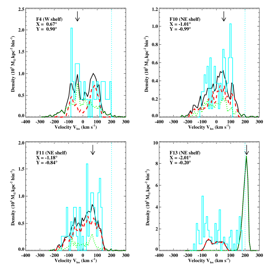
Figure 6: Same as Figure 5 for the four spectroscopic fields observed for RGB star velocities by Ibata et al. (2005) that lie in the shelf regions. Otherwise the caption to the previous figure applies here. The observational histograms are generated by taking the histogram of “disk lag velocity” in Ibata et al. (2005) and shifting by the velocity in their model of the disk at the center of the field. This neglects the slight variation of the disk velocity across the field. In these observational histograms, stars with positive velocities greater than $200\,\mbox{km}\,\mbox{s}^{-1}$ relative to M31 are removed to reduce Galactic contamination, as indicated by the dotted line. The observations show evidence for satellite debris in at least Panels (a) and (d), as discussed in the text.

In F4, F10, F11, and F13, stars are detected in a broad velocity distribution up to $|v|\sim 200\,\mbox{km}\,\mbox{s}^{-1}$ relative to M31, as shown by the light cyan histograms in Figure 6. A glance at Figure 6 shows that in fields F10 and F11, the predicted satellite and static M31 velocity distributions are actually fairly similar. Thus, the velocity distribution in these two fields cannot serve as evidence for or against our scenario without a deeper understanding of the slight differences. The histograms from the simulations suggest that the satellite debris dominates the distribution in both fields; differences in the stellar populations might serve to test this result, though this also could be difficult as these differences are quite subtle at this radius (Ferguson et al., 2005; Brown et al., 2006a, b).

In field F4, the strongly bimodal satellite distribution biased to positive velocities improves the agreement between the simulated and observed velocities, though the observed distribution extends to even higher velocities than shown by the simulated satellite debris. It is worth noting that the problem of foreground MW dwarf contamination increases with the velocity. The observed and simulated results in field F13 are similar to those in H13d above; again there is a population of observed stars at negative velocities, which are explained fairly well with the satellite debris. These two fields are thus encouraging for the debris model.

Field F13 also resembles Field H13d in that there is a strong predicted galaxy disk peak that is not seen in the observations. Once again there may be a smaller disk peak shifted to lower velocity by 40–$60\,\mbox{km}\,\mbox{s}^{-1}$. The velocity cut at $200\,\mbox{km}\,\mbox{s}^{-1}$ imposed by Ibata et al. to select M31 stars could be responsible for at least part of the difference, as it would remove many (though not all) disk stars in our $N$-body model for M31. Moreover, the warp of M31’s disk, which is quite strong this far along the NE major axis, may cause the disk contribution to be substantially lower in field F13 than in H13d (F13 being slightly off the major axis in the direction away from the warp). However, the H I in this region shows a peak at $220\,\mbox{km}\,\mbox{s}^{-1}$ (Newton & Emerson, 1977), exactly as predicted by the disk model, even though the H I disk itself is warped. A further possibility is that unlike the H I, the stellar velocities are perturbed from circular orbits. The extended disk found by Ibata et al. (2005) shows large velocity and density fluctuations relative to a smooth disk, and the results in fields H13d and F13 may be a further example of these fluctuations. A difference in H I and stellar velocities might be expected if the extended stellar disk resulted from an accreting satellite, as in the model of (Peñarrubia, 2006).

In summary, it appears that the debris model studied here explains a number of irregularities seen in the spatial and velocity distribution of the stars and PNe in and around M31. The strongest pieces of evidence for the model are the shape of the NE shelf on the sky, the apparent stream of counterrotating PNe and RGB stars seen along the NE major axis, and the agreement of the W shelf in the model with the spatial pattern seen in RGB stars and the kinematic distribution of PNe in the same area. The measured distance to the NE shelf stars is also consistent with our model. The fields observed for RGB velocities to date are not in regions that are optimal for testing the model, even though the existing fields are encouraging for the debris model, so we can anticipate great improvement in the observational constraints on this model. We now examine how future observations can test the model for the debris pattern, how we can understand its origin physically, and how we can use the debris to better understand M31 and its environment.

4 PHYSICAL INTERPRETATION AND DIAGNOSTICS

4.1 Model for collisionless shell systems

The NE and W shelves in our model appear similar to the “shells” observed around a significant fraction of elliptical and S0 galaxies. One mechanism for forming shells involves the disruption and folding of a thin, cold disk (Quinn, 1984; Hernquist & Quinn, 1988; Barnes & Hernquist, 1992). This scenario may well occur in nature, but it would tend to produce sharp, asymmetric features with no clear orientation around the galaxy center (for example, see Figure 3 of Quinn, 1984), and hence be a poor fit to the best-defined examples of shell patterns in ellipticals, as well as the tangentially oriented shelves discussed here. A more likely creation mechanism in our case is the accretion of a satellite on a nearly radial trajectory (e.g., Schweizer, 1980; Hernquist & Quinn, 1988; Barnes & Hernquist, 1992). Once the satellite is disrupted in whole or in part by its first close passage, the correlation between orbital energy and orbital period sorts the newly unbound stars in order of energy into a dynamically cold stream, with the lowest-energy stars executing the smallest and fastest orbits. The cooling of the stream means the progenitor need not itself be dynamically cold to produce a coherent shell, though this is possible as well. Subsequent passages near the center of the galaxy, combined with the dispersion in the angular momenta of the stars, disperse the stream stars in a variety of directions. The energetic sorting ensures that they nevertheless reach turnaround at a similar radius at any given time. This ongoing phase-wrapping process creates a series of caustic or “fold” features located on spherical shells, whose radii decrease along the orbit.

This scenario is much like our current understanding of the creation of M31’s southern stream (Ibata et al., 2001, 2004; Font et al., 2006; Paper I). Hence shell-like features are expected in M31 as long as the debris extends far enough ahead of the stream. The previous section provides evidence that this is indeed the case. In this subsection we discuss in more depth the physical properties of radial shells.

4.1.1 Stellar orbits in shell systems

To provide a concrete and analytically tractable example, let us make a number of approximations. First, we assume a power-law potential for the primary galaxy with $\Phi(r)\propto-r^{k}$. In Paper II, we found this was a reasonable approximation to the actual potential of M31 in the radial range 3–$100\,\mbox{kpc}$, with $k\approx-0.4$.

When the satellite collides with the primary galaxy, the tidal forces alter the energies of stars depending on their positions and orbits within the satellite, much like the gravitational slingshot of a planetary probe. In turn, the dispersion in their specific energies is related to the progenitor satellite’s mass $M_{s}$ and pericenter $r_{p}$, as found in Johnston (1998) and confimed by the simulations in Paper II. Using the latter simulations we estimate

$$\sigma_{E}\approx 0.7V_{c}^{2}(r_{p})\left(\frac{GM_{s}}{r_{p}V_{c}^{2}(r_{p})}\right)^{1/3}\;,$$ (1)

which we also found to be valid for our run in this paper. Here $V_{c}(r)=(GM(r)/r)^{1/2}$ is the circular velocity. The dispersion then increases with decreasing $r_{p}$. The combined requirements of a large dispersion in the energy and large angular deflections at pericenter explains why shell systems are most easily modeled using satellites with small $r_{p}$, i.e., on nearly radial orbits. We should note that we have not tested the validity of Equation 1 outside the regime of nearly radial orbits and an M31-like potential.

Next, we assume the newly liberated stars travel on purely radial orbits, i.e., we ignore the angular momentum. This is sufficiently accurate in our scenario, where the unperturbed orbit of our progenitor has a pericenter 45 kpc and apocenter 2 kpc. The stars then take on orbits that are described by the energy alone, or equivalently their orbital periods $t_{r}$. Let the turnaround radius of the progenitor be $r_{t0}$ and the circular velocity there be $V_{t0}$. Then $V_{c}(r)=V_{t0}(r/r_{t0})^{k/2}$.

For an arbitrary star, let us define a time scaling factor $\tau$ proportional to the orbital period of the star, $\tau=t_{r}/t_{r0}$. The self-similar nature of the orbit family leads to the scalings $r_{t}\propto\tau^{2/(2-k)}$, $V_{t}\propto\tau^{k/(2-k)}$, and $E\propto\tau^{2k/(2-k)}$. Stars with lower energies move faster, as long as $k<0$. The radius and velocity of a star with a given $\tau$ can be obtained from the orbital trajectory of the progenitor using the relations

$$r(t) = \tau^{2/(2-k)}r_{0}(t/\tau)\;,$$ (2)

$$v(t) = \tau^{k/(2-k)}v_{0}(t/\tau)\;.$$ (3)

Here we are treating the progenitor as a test particle, i.e., we ignore any change in the progenitor’s orbit from tidal disruption and dynamical friction. The exact orbital period of the star is

$$t_{r}=\sqrt{\frac{2}{(-k)}}\,B[1/2,(2-k)/(-2k)]\frac{r_{t}}{V_{t}}$$ (4)

where $B$ is the beta function.

The turnaround radius of a shell is found for $dr/d\tau=0$, which results in the requirement

$$\frac{t}{\tau}v_{0}(t/\tau)-\frac{2}{2-k}r_{0}(t/\tau)=0\;;$$ (5)

solving for the roots of this equation yields a series of spherical shells at fixed orbital phases. The radius of the shell at a given orbital phase is then $r_{s}=\tau^{2/(2-k)}r_{0}(t/\tau)\propto t^{2/(2-k)}$. The shell moves outwards with time, as stars with higher and higher energies arrive at the shell orbital phase. The ratio of the radii of two different shells is constant with time. These results are specific to the power-law potential, but also give a sense of the shell properties in the more general case.

4.1.2 Idealized surface density

To understand the sky pattern of a shell system, we must realize that the stars in a given shell may cover only a small fraction of the sphere, particularly early in its history as is the case for our simulation (cf. Figure 2). The observed properties of the shell depend on whether or not the shell surface lies tangent to the line of sight anywhere. These two cases are illustrated in Figure 7.

If the shell surface is tangent to the line of sight, as in the leftmost shell in the figure, then the caustic feature at turnaround is visible in projection as a circular boundary of the shell material. Let us here neglect locally the variation of the energy and mass flow rate along the stream. All stars in such a stream share the same shell radius $r_{s}$. Near this shell radius, the velocity of a star as a function of time $t$ is given by $dr/dt\approx-r_{s}^{-1}V_{c}^{2}(r_{s})(t-t_{s})=-\sqrt{2}V_{c}(r_{s})[(r_{s}-r)/{r_{s}}]^{1/2}$, where $r(t_{s})=r_{s}$ and $V_{c}$ is the circular velocity. Combining the inflowing and outflowing stars, we use this to derive the mass density of stars as a function of radius:

$$\rho(r)\approx\frac{2}{4\pi r^{2}|dr/dt|}\frac{dM}{dt}\;\\ \approx\frac{1}{2^{3/2}\pi\,f_{\Omega}\,r^{2}\,V_{c}(r_{s})}\,\left(\frac{r_{s}-r}{r_{s}}\right)^{-1/2}\,\frac{dM}{dt}\,.$$

Here $dM/dt$ is the rate at which mass flows through the stream (for example, the amount of mass that reaches apocenter per unit time). $f_{\Omega}$ is the fraction of the total $4\pi$ sr of the sphere that the shell covers; put another way, it specifies the ratio of the local mass flow rate per unit solid angle to its average over the sphere.

When integrated over constant projected radius, this gives the result that the mass surface density $\Sigma$ approaches a constant just inside the shell radius,

$$\Sigma(r_{s})=\frac{f_{\theta}}{2\,f_{\Omega}\,r_{s}\,V_{c}(r_{s})}\frac{dM}{dt}\;,$$ (6)

and drops to zero outside of it. Here $f_{\theta}$ represents the fraction of the mass that is present along the line of sight compared to a full spherical shell; at the shell radius $f_{\theta}=1$ (otherwise it would not even be visible), but it can drop off at smaller radii, as can be seen in the leftmost shell in Figure 7. This factor partially compensates for the solid angle factor $f_{\Omega}$. The reason for the constant surface density at the edge is that as the line of sight moves inward from the shell edge, it reaches a smaller minimum radius, but also takes a shorter (increasingly vertical) path through the material at the edge of the shell; these two effects cancel each other out. The relationship just derived allows us to obtain the local mass flow rate from the surface brightness of the shell, which we make use of in § 4.4. (Hernquist & Quinn, 1988 previously noted that the surface density approaches a constant, without relating it to dynamical quantities.)

If the shell surface is not tangent anywhere to the line of sight, as in the rightmost shell in Figure 7, then the extent of the shell in projection is limited by the angular coverage rather than the shell radius. The dropoff outside the shell region need not be sharp, and the boundary of the shell on the sky need not be a circular arc. The surface density in this case can be estimated from the average over the sphere. A single spherical shell corresponds to a single orbit, so the total mass contained within the shell equals $t_{r}dM/dt$, where $t_{r}$ is given by Equation 4. The total surface area of a full spherical shell on the sky is $\pi r_{s}^{2}$, so the average surface density is

$$\Sigma_{avg}(r_{s})\approx\frac{1}{\pi}\sqrt{\frac{2}{(-k)}}\,B[1/2,(2-k)/(-2k)]\frac{f_{\theta}}{f_{\Omega}\,r_{s}\,V_{c}(r_{s})}\frac{dM}{dt}\;,$$ (7)

where we have included corrections for the angular coverage as before. For $k=-0.4$, the constant in front is 0.76, slightly exceeding the value of 0.5 obtained at a true shell edge (c.f. Equation 6), although typically the value of $f_{\theta}$ will also be smaller than at an edge. Thus there is no strong limb brightening or darkening; the surface density does not depend very much on whether the line of sight is at a true edge or not.

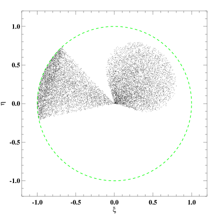
Figure 7: Idealized illustration of partial shells in a spherical potential. Two shells are shown, which are identical except in their orientation. Each shell fills a cone with an opening angle of $30^{\circ}$; the radial distribution assumes a steady stream in a power-law potential. The leftmost shell is tangent to the line of sight, and thus its outer boundary on the sky is defined by the shell radius. Note the dark region where the shell’s “end cap” is visible. The rightmost shell is not tangent to the line of sight, and as a result has a less distinct edge, and a boundary that varies in projected radius.

4.1.3 Idealized velocity pattern

Merrifield & Kuijken (1998, henceforth MK) studied the kinematics of shells. They assumed a shell composed of stars on monoenergetic, low-angular-momentum orbits lying tangent to the line of sight. They then found that these stars have a characteristic kinematic signature, which depends only on the shell radius and the total mass contained within it. In the space of line-of-sight velocity $v_{los}$ versus projected radius $R$, the MK result is that stars near the shell radius inhabit a region with a triangular boundary:

$$|v_{los}|\leq V_{c}(r_{s})\,\frac{r_{s}-R}{r_{s}}\;.$$ (8)

The stars fill this region unevenly, congregating at the boundary. This boundary is again a caustic feature, which forms because the velocity component in the line-of-sight direction $\hat{z}$ goes to zero at both $z=0$ and $r=r_{s}$, so it must reach an extremum at some intermediate point along the line of sight.

For the discussion below, it is important to understand the relationship between the position and velocity of the stars. We illustrate this in Figure 8 for a full spherical shell. The region in physical space that corresponds to the velocity caustic is marked by a red line. Caustics occur at positive velocities in two sets of stars: outbound stars lying more distant than the galaxy center, and inbound stars lying in front of the galaxy center. There are negative-velocity caustics made up of the other two combinations.

In the case considered by MK, the velocity distribution is symmetric around zero, so that the slope is equal and opposite on the positive and negative velocity sides, and $v_{los}=0$ at $r_{s}$. Also, there is a degeneracy between the stars on the near and far sides of the galaxy; outbound stars with $z<0$ have the same sign and distribution in velocity as inbound stars with $z>0$, and vice versa. Several effects may break this degeneracy in a more realistic case, as discussed below. The method suggested by MK has not yet been applied to measure the potential in observed shell galaxies, due to the low surface brightness of the shells and the difficulty in estimating the bimodal velocity signature from weak absorption lines.

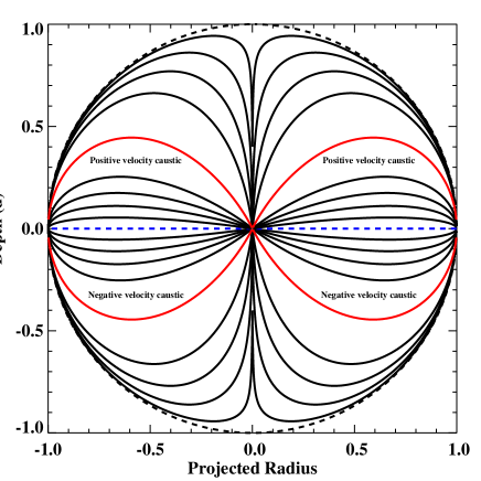
Figure 8: Location of the velocity caustics, in an idealized model of a spherical shell of stars. Here we assume a spherical, power-law potential with $\Phi\propto-r^{-0.4}$, and a monoenergetic stream. Projected radius $R_{proj}$ and line-of-sight distance $d$ are plotted in units of the shell radius. We have reflected the pattern around the vertical axis. Since the shell geometry is spherically symmetric, rotating the entire figure around the vertical axis gives the full three-dimensional pattern. The shell boundary is shown by the dashed line. The contours show the the line-of-sight velocity relative to the maximum velocity along each line of sight, i.e., at a fixed $R_{proj}$; contour values are at ($-1$,$-0.8$,$-0.6$…0.6,0.8,1). The maximum and minimum velocities along each line of sight occur on the caustics marked with red lines, which are labeled appropriately for the outgoing stars. For the incoming stars the labels would be reversed.

4.2 3-D geometry of the debris in M31

In the discussion above, we have emphasized the role played by the angular coverage of the shells. This is important in our model since the shell features cover nowhere near the full extent of the sphere, as can be seen in Figure 2. It is worth taking a closer look at the origin and effects of the spatial structure.

In our simulations, the NE shelf is made up of both material from the leading stream from the first pericentric passage, which is spread out into a flattened structure at the second pericentric passage, and material stripped from the remnant of the progenitor at its second pericentric passage, when it completely disrupts. The disruption is largely a product of the central density chosen in our initial conditions, since a more concentrated satellite survived the same passage in one of our test runs. While complete disruption is in accord with the lack of an obvious visible progenitor, it is not required in order to reproduce the shelves. The forward stream is further distorted at the third pericentric passage into a conical structure, which forms the W shelf.

The solid angle covered by the simulated NE shelf debris is actually even more limited than is apparent in Figure 2. When viewed in three dimensions, it resembles a pair of fans joined at the edges, corresponding to the outbound and inbound sections; each of these fan layers is only a few kpc thick, as shown in the second panel of Figure 9. Because this portion of the debris shell does not lie tangent to the line of sight, its boundary viewed in projection is defined by the angular coverage and not the shell radius, and thus varies in projected radius as a function of azimuth. The latter property also seems to be shared by the observed NE shelf (see Figure 1 and Table 1), although further work is warranted to confirm this result.

The southern stream is observed out to near its turnaround radius, so its length scale is well constrained. Above we found that the radii of different shells maintain a fixed ratio with time. Since the southern stream is in essence the shell preceding the NE shelf, this suggests that the shell radii are highly robust for any model that fits the stream. Indeed, we found it difficult to change the shell radii significantly for simulations with acceptable stream properties, despite a variety of initial conditions and orbital phases.

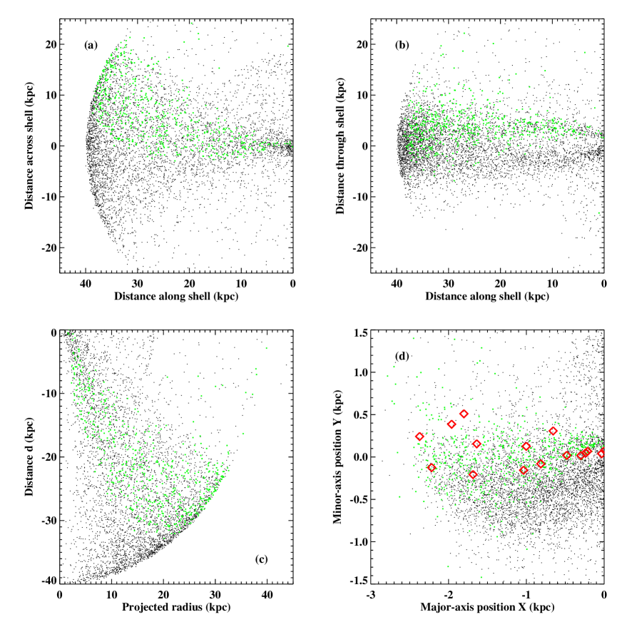
Figure 9: The NE shelf’s fan structure. In each panel, the dots indicate $N$-body particles; those designated as “Merrett PNe stream” particles in Figure 3 are marked in green. Panel a: the top view of the structure. M31’s center is located on the right at $(0,0)$. The horizontal axis points along the main axis of the structure away from M31, while the vertical axis points across the other elongated direction of the structure. Panel b: a side view of the NE shelf structure, at right angles to the previous panel. This clearly shows the outbound (top) and inbound (bottom) layers of the double fan structure. Again, M31’s center is on the right at coordinates $(0,0)$. Panel c: distance $d$ relative to M31, versus projected radius on the plane of the sky. Only those particles in the NE half of M31 ($X<0$) are shown. Compare the position of the “stream” particles here to the spatial region occupied by the velocity caustic in Figure 8. Panel d: the sky view of the NE shelf structure, plotted in M31 major and minor axis coordinates ($X$ and $Y$, respectively). The PNe designated by Merrett et al. (2006) as “Stream” or “Stream?” are marked by red diamonds, and overlay the analogous stream in the simulation.

The outbound fan on the E side overlaps the region of the velocity caustic, as seen in Figure 9. This leads to a new interpretation of the Merrett et al. PNe “stream”: it does not represent an isolated stream of stars traveling along a single path, but rather represents an intersection between an approximately two-dimensional distribution of stars and the mainly two-dimensional region of space where the velocity caustic occurs. The various panels of Figure 9 indicate in green the “PNe stream” simulation particles previously marked in Figure 3. The red symbols in the last panel show the location on the sky of the “stream” PNe found by Merrett et al., which agree well with the location of our apparent stream. From the top view of the structure (Figure 9c), however, it can be seen that the “PNe stream” particles do not form an isolated density concentration, and actually inhabit a slightly curved region on the fan structure rather than following a single orbit. The “PNe stream” stars therefore just constitute a portion of a larger structure, singled out by the kinematics in projection along the line of sight.

The inbound portion of the fan has its own, inbound “stream”, which is offset about $0.5^{\circ}$ to the SW of the outbound “stream”. This unfortunately mainly lies just outside the region surveyed by Merrett et al. for $X<-1.0^{\circ}$, and for $X>-1.0^{\circ}$ the velocities mainly lie within the range expected from disk stars. However, this returning stream should be detectable in a wider PNe survey or a sufficiently large RGB sample. A sample near $\xi\approx 1.7^{\circ}$, $\eta\approx 0.7^{\circ}$ may separate the returning component from the disk spatially, while a sample near $\xi\approx 1.6^{\circ}$, $\eta\approx 1.2^{\circ}$ may separate it kinematically as it should have a lower velocity there than that of the disk. The existence of a returning stream is a critical test of the scenario in this paper, since it links the outbound NE shelf stars to the W shelf.

The W shelf in our simulation is much less flattened than the NE shelf, and hence looks more like our idealized notion of a shell in Figure 7. The majority of the stars lie within a cone $60^{\circ}$–$90^{\circ}$ wide, though many of the stars still lie on a curved concentration on one side of this cone. The inbound and outbound stars are intermingled, and some of the inbound stars have been scattered far outside of the main conical region. The stream connecting the E and W stars passes very close ($\la 1\,\mbox{kpc}$) to M31’s center in this simulation, which helps account for the increased scatter in orbit directions. The main body of the shelf lies more distant than M31’s center, and is viewed edge-on over much of its apparent outer boundary, which explains the relatively sharp and circular appearance in Figure 2.

We note that there is yet another radial shell of debris in our model, consisting of particles even further forward than those in the W shelf. This shell is very faint, as it contains only about $6\times 10^{7}\,M_{\sun}$, which is only about a tenth as much mass as the shell making up the W shelf. This result is highly model-dependent, since this shell represents the extreme forward edge of the satellite debris. The shell may not exist at all, or may be much more massive than found in our simulation. The particles in this shell cover the entire E side of M31 fairly evenly, out to a radius of $18\,\mbox{kpc}$. Deep kinematic surveys around the SE minor axis would seem to be the method most likely to detect this debris.

4.3 Velocity pattern: expectations and relation to M31’s potential

Velocity measurements of the shell debris, as discussed by MK, are potentially the most powerful constraints on acceptable models of their makeup. This is partly because velocities can be measured much more accurately than distances, and partly because the velocities are extremely coherent. Figure 10a shows the location of the particles in the space of M31-centric radius versus M31-centric radial velocity. The particles occupy a cold stream, which spirals in the clockwise direction as one goes further forward in the stream. The southern stream, NE shelf, and W shelf are easily seen as the first three groups of particles starting from the right. The fainter shelf just described on the eastern side is seen as the fourth group. The energy decreases along the stream, reducing the apocentric radii of successive radial loops.

In qualitative accord with the predictions of MK discussed above, we find that the velocities lie within a well-defined, roughly triangular region in the space of $v_{los}$ versus $R_{proj}$, as shown in Figure 10 (see also the similar Figure 4b). Over most of the region, the velocity distribution has two peaks at positive and negative velocity, which both approach $v\approx 0$ (using velocity relative to M31) as $R_{proj}$ approaches the shelf boundary. These two peaks are shown clearly in the histograms of the velocity distribution in Figure 11. These two peaks generally have unequal strength, particularly at small radii in the W shelf where the negative-velocity peak is a fraction of its positive-velocity counterpart. The returning or positive-velocity “stream” in the NE shelf shows up quite clearly in this representation. As mentioned above, this component has so far eluded detection, probably due mostly to the areal coverage of the kinematic surveys.

This velocity pattern will be easiest to recognize near the edges of the shelf, in the regions far away from M31’s disk. We discussed evidence that portions of this pattern are visible in existing observations in § 3.3, including the apparent outbound “stream” in the NE shelf. The corresponding inbound stream is more easily seen in Figures 10 and 11 than in Figure 3, both because the division at $Y=-0.3^{\circ}$ splits the stream particles between the two panels of the latter figure, and because the line-of-sight velocity is a function of $R_{proj}$ rather than $X$, and those two quantities are not well aligned in the main region occupied by the inbound stream.

We fit the upper and lower envelopes in panels (b) and (c) of Figure 10 with straight lines, using only the outer portions of each shelf. Using MK’s approximation in Equation 8, we obtain estimated circular velocities of $291\,\mbox{km}\,\mbox{s}^{-1}$ in the NE shelf at 36 kpc from M31, and $245\,\mbox{km}\,\mbox{s}^{-1}$ in the W shelf at 24 kpc. The actual circular velocities at these two radii in our potential model are 214 and 229 kpc, respectively. Thus, the MK prediction is not in precise quantitative accord with the simulation, but rather overestimates the enclosed mass by 15–85%. There are other disagreements with the MK description as well: the velocity slopes are not equal and opposite, and the tip velocity is nonzero.

Using the simulation particles, we find that these discrepancies originate from several effects not considered by MK, including the following: the nonzero angular momentum in the debris; the significant gradient of energy along the stream; the continuing dynamical interaction with the progenitor, mainly in the NE shelf; perspective effects from the large size and small distance of the M31 system; and finally, the finite range of radius needed to measure the slope. All of these effects change the velocities visibly in Figure 10, and taken together change the measured slope significantly. They also break the above-mentioned symmetry between the caustics from particles on opposite sides of M31, though the particle distribution is so heavily weighted to one side in each case that this effect is barely visible. In both shells, the limited spatial coverage of the shell does not greatly modify the slope of the velocity envelope, although the lack of stars near the shell edge does deplete the region near the tip and make the slope measurement more challenging.

Despite these complications, the general point of the MK paper is still valid: the velocity signature in shells can serve as a useful diagnostic of the gravitational potential, over a radial range 15–$35\,\mbox{kpc}$ in this case. Our gravitational potential is not necessarily the correct one. We expect the measurement biases to be similar for different potentials though, so to first order the ratio found here between predicted and measured velocity gradients can be used to estimate the true enclosed mass at the shelf radii. Measurements of the H I rotation curve now probe out to $\approx 35\,\mbox{kpc}$ as well (Carignan et al., 2006), but there are significant concerns about these results due to the warping and irregular structure of the disk. Hence, the shelf velocities will help confirm the H I measurements, and will also allow comparison of the potential in and out of the plane, thereby constraining the ellipticity of the dark matter distribution.

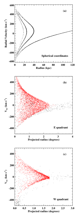
Figure 10: Panel a: M31-centric radial velocity versus M31-centric radius for the satellite debris particles in the simulation. The southern, trailing stream is made up of the long tail to large radius, while the debris further forward spirals clockwise in a series of radial loops. The NE shelf is made up of the particles in the largest complete loop, out to 40 kpc, while the W shelf is made up of the particles in the next loop. Panel b: Line-of-sight velocity versus projected radius, showing only particles in the quadrant $X_{M31}<0$, $Y_{M31}<0$ containing the NE shelf. Particles genuinely in the radial shell corresponding to the NE shelf are marked with red dots. The black dots show particles belonging to other radial shells; these are mostly spillover from the southern stream, though some debris further forward than the W shelf is also present at small radii. Note that in this projection, the returning “stream” in the NE shelf (the concentration at the upper edge of the red particles) is more easily seen than in Figure 3. Panel c: Same as Panel b, but showing particles in the quadrant $X_{M31}>0$, $Y_{M31}>0$ containing the W shelf. Particles genuinely in the radial shell corresponding to the W shelf are marked with red dots. Other particles, mostly spillover from the NE shelf, are shown as black dots.

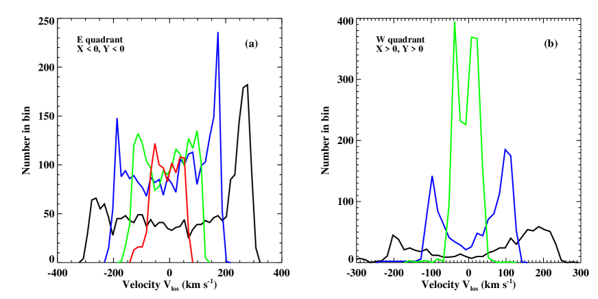
Figure 11: Histograms of the line-of-sight velocity of satellite debris particles at different projected radii. Left panel: Particles in the quadrant $X_{M31}<0$, $Y_{M31}<0$ containing the NE shelf. Curves show results for $0.5^{\circ}<R_{proj}<0.6^{\circ}$ (black), $1.0^{\circ}<R_{proj}<1.1^{\circ}$ (blue), $1.5^{\circ}<R_{proj}<1.6^{\circ}$ (green), $2.0^{\circ}<R_{proj}<2.1^{\circ}$ (red). Right panel: Same, for the quadrant $X_{M31}>0$, $Y_{M31}>0$ containing the W shelf. Curves show results for $0.5^{\circ}<R_{proj}<0.6^{\circ}$ (black), $1.0^{\circ}<R_{proj}<1.1^{\circ}$ (blue), $1.5^{\circ}<R_{proj}<1.6^{\circ}$ (green).

4.4 Surface density profile as a diagnostic of the progenitor

We now investigate what the surface density of the shelves signifies for the position and mass of the progenitor. First, we check the approximate relationship between the surface density and the mass flow rate, using the simulated W shelf as a test case. Equation 6 is the appropriate form to use for this shelf since it is nearly tangent to the line of sight. In § 3.2 we found the simulated surface density in the W shelf was $\Sigma_{W}=7.2\times 10^{5}\,M_{\sun}\,\mbox{kpc}^{-2}$. For the other constants in Equation 6 we find $r_{s}\approx 25\,\mbox{kpc}$, $V_{c}\approx 230\,\mbox{km}\,\mbox{s}^{-1}$, and $dM/dt\approx 1.6\,M_{\sun}\,\mbox{yr}^{-1}$, using the rate of mass in the shell reaching turnaround as an estimate of the latter quantity. Converting the particles in this radial shell into a fully spherical shell by randomizing their orientations relative to M31, and computing the surface density in the W shelf region as before, we find a surface density of $1.5\times 10^{5}\,M_{\sun}$. This is about 5 times smaller than the actual simulated density, implying $f_{\theta}/f_{\Omega}=5$ in Equation 6, which is the appropriate form to use for the W shelf since it is nearly tangent to the line of sight. The expected surface density of the W shelf is then $\approx 6.3\times 10^{5}\,M_{\sun}\,\mbox{kpc}^{-2}$, consistent with the actual surface density in the simulation within the limits of our accuracy. Predicting the NE shelf surface density is potentially more complicated, since it may contain contributions from both the first and second pericentric passages of the progenitor satellite, so we will not make use of it here.

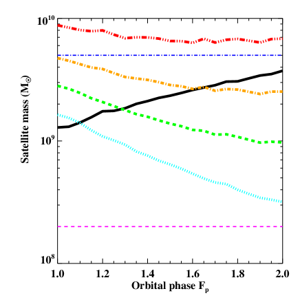
Figure 12: Estimates of the progenitor’s mass at the time it disrupts to form the stream, as a function of the progenitor’s current orbital phase. The orbital phase is defined in units of the progenitor’s radial orbital period, starting from the time of disruption. The derivations of the various estimates are discussed in the text. Rising solid curve: estimate from stellar mass in the stream, accounting for the mass outside the stream. Falling curves: estimates from the surface density in the W shelf, using surface densities of 2, 4, 8, and $16\times 10^{5}\,M_{\sun}\,\mbox{kpc}^{-2}$ from bottom to top. Horizontal dashed line: estimate of stellar mass in the stream alone. Horizontal dot-dashed line: estimate from the metallicity of stream stars (Font et al., 2006). With a better-constrained W shelf surface density, the intersection of the rising and falling curves can be used to constrain the progenitor mass and current orbital phase.

By viewing successive snapshots of our $N$-body simulation, we can easily see that the surface density in the W shell increases with time, because the mass flow rate in the stream $dM/dt$ is also increasing as the progenitor approaches closer to this point in the orbit. This suggests that we can use the shelf surface brightness to constrain the progenitor mass and orbital phase. In Paper II, we put limits on the mass and phase using properties of the southern stream alone. The basic idea was that given a progenitor phase, the progenitor mass sets both the overall normalization and the phase extent of the stream mass, and hence the fraction of the mass in the visible extent of the southern stream. This argument was limited in its power, though, because a larger progenitor phase could always be compensated for by a larger progenitor mass. With the detection of the W shelf, it seems that the progenitor phase can be limited from the other direction, effectively triangulating its position.

We proceed similarly to §3.2 in Paper II. We fit a sequence of trajectories assuming different present-day progenitor phases $F_{p}$, and otherwise following the method of §3.1 above. For each fit, we calculate the time scaling factor $\tau$ at the W shelf and at Fields 4 and 8 of McConnachie et al. (2003) within the southern stream, which span the same radial range as that used by Ibata et al. (2001) in calculating the stream’s luminosity. We also calculate the progenitor’s orbital energy $E_{0}$, its progenitor’s radial period $t_{r0}$, its pericentric radius $r_{p}$, the W shell radius $r_{s}$, and the circular velocity at $r_{p}$ and $r_{s}$.

For the distribution of orbital energy in the debris, $\chi(E)$, we adopt a Gaussian form with the dispersion $\sigma_{E}$ given in Equation 1. This form is a reasonably accurate approximation to the simulations in Paper II and this paper, and an improvement on the top hat distribution used in Fardal et al. We estimate the energies at Fields 4 and 8 as $E_{4}=E_{0}\tau_{4}^{-1/3}$ and $E_{8}=E_{0}\tau_{8}^{-1/3}$, using the scalings above with $k=-0.4$. We take the total mass of the stream between fields 4 and 8 as $M_{\it stream}\approx 2\times 10^{8}\,M_{\sun}$, as discussed in § 3.2. We then estimate the mass of the progenitor satellite $M_{s}$ from that of the stream by solving the following equation:

$$M_{s}\int_{E_{8}}^{E_{4}}\chi(E)\,dE=M_{\it stream}\;.$$ (9)

This result is shown by the solid curve in Figure 12.

We then estimate $M_{s}$ independently from the surface density of the W shelf using Equation 6. We relate the mass flow rate at the edge of the shelf to the steadily increasing energy there using

$$\frac{dM}{dt}=M_{s}\chi(E)\frac{dE}{dt}\;,$$

where the change in energy per unit time $t$ at a fixed orbital phase is

$$\frac{dE}{dt}=\frac{dE}{d\tau}\frac{d\tau}{dt}\approx-\frac{E}{3t}\;.$$

Combining these results with Equation 6, we get an equation that can be solved for the progenitor satellite’s mass $M_{s}$:

$$M_{s}\frac{dE}{dt}(\tau_{sh})\chi(E)=2\frac{f_{\Omega}}{f_{\theta}}r_{sh}V_{c}(r_{sh})\Sigma(r_{sh})\;.$$ (10)

Here we take $f_{\theta}/f_{\Omega}=5$, as found using the simulated debris. In Figure 12 we provide four curves using shell surface densities of $\Sigma_{W}=2$, 4, 8, and $16\times 10^{5}\,M_{\sun}\,\mbox{kpc}^{-2}$, which probably cover the allowed range ($8\times 10^{5}$ is our most likely value, although this includes the smooth halo component of M31).

The estimate of the progenitor mass and phase is then given by the point where the W shelf curve, for an observed $\Sigma_{W}$, crosses the solid curve from the stream mass. Both analytic estimates use a series of approximations and may be imprecise by perhaps a factor of two. Also, assuming that the stripped fraction or baryonic fraction in the progenitor is less than unity will raise both mass estimates together. The plot suggests a minimum progenitor mass of $M_{s}\ga 1.5$–$5\times 10^{9}\,M_{\sun}$, depending on the shelf surface density. These masses are consistent with our simulation and with the estimate of the progenitor mass from the metallicity (Font et al., 2006), shown as the upper horizontal line. On the other hand, these estimates are far above the integrated mass in the stream itself, shown as the lower horizontal line.

The progenitor’s orbital phase can already be limited to $F_{p}\ga 1.1$, according to the plot. The plot also shows that $F_{p}$ can be determined within a small fraction of a radial period, once the surface density in the W shelf is known precisely.

The constraints given here can be improved in the future by using surface density constraints all the way out to the tip of the southern stream, and by using an ensemble of $N$-body simulations to avoid the need for analytic approximations. Nevertheless, it should be clear from this discussion that the surface density distribution is an important clue to the orbital and physical parameters of the progenitor.

5 DISCUSSION

We have performed a simple $N$-body simulation in the gravitational potential of M31, and used this to show that an accreting satellite can explain the giant southern stream, the eastern shelf, and a similar shelf on the western side as a single continuous structure. Following the entire folded path traced by the stream and shelf particles, the structure is $\ga 230\,\mbox{kpc}$ long, certainly among the largest coherent stellar structures known despite its modest total stellar mass of $\sim 2\times 10^{9}\,M_{\sun}$. The NE and W shelves in this model represent successive radial loops of the orbit broadened into fan shapes by passage through pericenter. The NE shelf lies closer to us than the disk of M31, and partially overlaps with it. This may have relevance to microlensing surveys which aim to detect compact objects of stellar-type mass (Calchi Novati et al., 2005; de Jong et al., 2004), since the lensing event probability will be boosted relative to disk self-lensing by the gap in distance between the disk and NE shelf, and by the large relative velocities between the disk and shelf stars.

The counter-rotating “stream” in the NE seen in both PNe and RGB stars in this view represents a continuation of the NE shelf onto the face of M31, while the apparently narrow velocity width of this stream is explained by a caustic in velocity space. The properties of the incoming satellite are reasonable for a galaxy of its initial stellar mass, as discussed in § 3.1. While we have not explored velocity distributions outside the shelf regions in detail, our impression is that the model is satisfactory in terms of where it does not put debris, as well as where it does. Our experience with different initial conditions (in Paper II) suggests that this would not necessarily be true for orbits that tried to associate the southern stream with other objects such as M32 or the Northern Spur.

We experimented with low-resolution versions of our main run, testing different orbits and satellite properties. Our sense acquired during this exploration is that the volume of parameter space that can match current observations is large enough not to need extreme fine-tuning. The time corresponding to “present day” within our run is uncertain by perhaps 100 Myr, and it is not clear whether the progenitor need be disrupted or not. As surveys of M31’s disk and halo regions continue, we expect that the requirements on the model will become much more stringent.

We remind the reader that we have neglected several physical effects in computing this model that are potentially important. These include dynamical friction, the response of the modes in the disk, rotation of the accreting satellite, dark matter in and around its stellar component, and the hydrodynamic interaction of gas within the satellite with the disk and halo of M31. In addition, the observations do not yet cover some of the most interesting areas for this model, and our comparison to the existing observations is as yet rudimentary. We therefore regard the existing simulation as a useful illustration, rather than a definitive prediction of the debris structure. Work on the interaction of the satellite with live dynamical components of M31 is currently underway.

Kinematic observations in the shelf regions are important for two reasons. First, they can help clarify the nature and extent of the debris related to the giant southern stream. The many testable predictions of our model include:

• The “PNe stream” of Merrett et al. (2006) should be continuously connected to the NE shelf, since in our model it is merely a region where the kinematics in projection gives a roughly constant velocity, and not a separate structure.

• In both shelves, the characteristic kinematic pattern of a shell should be evident in the $R_{proj}$–$v_{los}$ plane (Figure 10).

• There should be stars with positive velocities returning to the center of M31 in the NE shelf, which connect the NE and W shelves.

• There may be a yet weaker shelf on the E side, from debris further forward in the stream.

Second, the velocity signature of the shells depend on the potential of M31. Many more spectroscopic fields will be required to allow a precise measurement of the potential. However, unlike the case of the collimated southern stream, the line-of-sight distances need not be computed at all to probe the potential of M31, as the geometry itself selects the stars in the velocity caustic. This removes one of the main sources of uncertainty in constraining the mass model. Comparison of the potential derived from the shelves to that obtained from H I rotation curves can help test the deviation of M31’s mass distribution from spherical symmetry.

If confirmed as shells connected to the southern stream, the NE and W shelves would to our knowledge represent the first detection of a multiple-shell system in a late-type spiral galaxy. Shells are very common in elliptical galaxies. 137 elliptical galaxies with shells were catalogued by Malin & Carter (1983), while Merrifield & Kuijken (1998) estimate that 10% of elliptical galaxies have shells. The reasons for this strong morphological bias have not been completely explained at present. Spirals may be destroyed and ellipticals created in the mergers that produced the shells, although this would only be plausible for merging systems much more massive than in the case discussed here (see Hernquist & Spergel, 1992, for a discussion of shell formation in major mergers). Alternatively, shells may dissolve faster in the non-spherical potential of the disk due to differential precession of the orbits. The difficulty of distinguishing shells from spiral features in late-type galaxies may also contribute to the lower rate of observing shells (Barnes & Hernquist, 1992). If all shells around spiral galaxies were as faint as the ones in M31, they would have escaped detection, since RGB star count maps like those of Ferguson et al. (2002) can be made only at close range. M31’s putative shell system would also be the first in which kinematic observations have been made, allowing us to compare to and eventually constrain mass models of the host galaxy.

Theoretical studies of dark halos have established their mean mass profile to high accuracy in the absence of baryons. Their response to the baryonic component in terms of their mass profile, ellipticity, and alignment with the disk is more difficult to simulate, making observational checks important. However, these aspects are difficult to study in most galaxies. The abundance in M31 of both coherent tracers of the potential, such as the tidal debris discussed in this paper, and statistical tracers such as RGB stars, satellite galaxies, and globular clusters, suggests that this galaxy can be a Rosetta Stone for understanding the properties of dark halos and their interaction with the galaxies they host.

References

- Barnes & Hernquist (1992) Barnes, J. E., & Hernquist, L. 1992, ARA&A, 30, 705
- Binney & Tremaine (1987) Binney, J. & Tremaine, S. 1987, “Galactic Dynamics”, Princeton University Press, Princeton, NJ
- Brown et al. (2006a) Brown, T. M., Smith, E., Guhathakurta, P., Rich, R. M., Ferguson, H. C., Renzini, A., Sweigart, A. V., & Kimble, R. A. 2006, ApJ, 636, L89
- Brown et al. (2006b) Brown, T. M., Smith, E., Ferguson, H. C., Guhathakurta, P., Renzini, A., Sweigart, A. V., & Kimble, R. A. 2006, accepted to ApJ (astro-ph/0607637)
- Calchi Novati et al. (2005) Calchi Novati, S., et al. 2005, A&A, 443, 911
- Carignan et al. (2006) Carignan, C., Chemin, L., Huchtmeier, W. K., & Lockman, F. J. 2006, ApJ, 641, L109
- Chapman et al. (2006) Chapman, S. C., et al. 2006, ApJ, in press (astro-ph/0602604)
- de Jong et al. (2004) de Jong, J. T. A., et al. 2004, A&A, 417, 461
- Dekel & Woo (2003) Dekel, A., & Woo, J. 2003, MNRAS, 344, 1131
- Fardal et al. (2006) Fardal, M. A., Babul, A., Geehan, J. J., & Guhathakurta, P. 2006, MNRAS, 366, 1012 (Paper II)
- Ferguson et al. (2002) Ferguson, A. M. N., Irwin, M. J., Ibata, R. A., Lewis, G. F., & Tanvir, N. R. 2002, AJ, 124, 1452
- Ferguson et al. (2005) Ferguson, A. M. N., Johnson, R. A., Faria, D. C., Irwin, M. J., Ibata, R. A., Johnston, K. V., Lewis, G. F., & Tanvir, N. R. 2005, ApJ, 622, L109
- Font et al. (2006) Font, A. S., Johnston, K. V., Guhathakurta, P., Majewski, S. R., & Rich, R. M. 2006, AJ, 131, 1436
- Geehan et al. (2006) Geehan, J. J., Fardal, M. A., Babul, A., Guhathakurta, P. 2006, MNRAS, 366, 996 (Paper I)
- Gilbert et al. (2006) Gilbert, K. M., et al. 2006, ApJ, in press (astro-ph/0605171)
- Guhathakurta et al. (2005) Guhathakurta, P., Ostheimer, J. C., Gilbert, K. M., Rich, R. M., Majewski, S. R., Kalirai, J. S., Reitzel, D. B., Cooper, M. C., and Patterson, R. J. 2005, arXiv preprint (astro-ph/0502366)
- Guhathakurta et al. (2006) Guhathakurta, P., Rich, R. M., Reitzel, D. B., Cooper, M. C., Gilbert, K., Majewski, S. R., Ostheimer, J. C., Geha, M. C., Johnston, K. V., & Patterson, R. J. 2006, AJ, 131, 2497
- Hernquist & Quinn (1988) Hernquist, L., & Quinn, P. J. 1988, ApJ, 331, 682
- Hernquist (1990) Hernquist, L. 1990, ApJ, 356, 359
- Hernquist & Spergel (1992) Hernquist, L., & Spergel, D. N. 1992, ApJ, 399, L117
- Ibata et al. (2001) Ibata, R., Irwin, M. J., Ferguson, A. M. N., Lewis, G., & Tanvir, N. 2001, Nature, 412, 49
- Ibata et al. (2004) Ibata, R., Chapman, S., Ferguson, A. M. N., Irwin, M., Lewis, G., & McConnachie, A. 2004, MNRAS, 351, 117
- Ibata et al. (2005) Ibata, R., Chapman, S., Ferguson, A. M. N., Lewis, G., Irwin, M., & Tanvir, N. 2005, ApJ, 634, 287
- Irwin et al. (2005) Irwin, M. J., Ferguson, A. M. N., Ibata, R. A., Lewis, G. F., & Tanvir, N. R. 2005, ApJ, 628, L105
- Johnston (1998) Johnston, K. V. 1998, ApJ, 495, 297
- Kalirai et al. (2006a) Kalirai, J. S., Gilbert, K. M., Guhathakurta, P., Majewski, S. R., Ostheimer, J. C., Rich, R. M., Cooper, M. C., Reitzel, D. B., and Patterson, R. J. 2006a, ApJ, in press (astro-ph/0605170)
- Kalirai et al. (2006b) Kalirai, J. S., Guhathakurta, P., Gilbert, K. M., Reitzel, D. B., Majewski, S. R., Rich, R. M., & Cooper, M. C. 2006b, ApJ, 641, 268
- Law, Johnston, & Majewski (2005) Law, D. R., Johnston, K. V., & Majewski, S. R. 2005, ApJ, 619, 807
- Lewis et al. (2004) Lewis, G. F., Ibata, R. A., Chapman, S. C., Ferguson, A. M. N., McConnachie, A. W., Irwin, M. J., & Tanvir, N. 2004, Publications of the Astronomical Society of Australia, 21, 203
- Malin & Carter (1983) Malin, D. F., & Carter, D. 1983, ApJ, 274, 534
- McConnachie et al. (2003) McConnachie, A. W., Irwin, M. J., Ibata, R. A., Ferguson, A. M. N., Lewis, G. F., & Tanvir, N. 2003, MNRAS, 343, 1335
- McConnachie et al. (2004) McConnachie, A., Ferguson, A., Huxor, A., Ibata, R., Irwin, M., Lewis, G., & Tanvir, N. 2004, The Newsletter of the Isaac Newton Group of Telescopes (ING Newsl.), 8, 8
- McConnachie et al. (2004) McConnachie, A. W., Irwin, M. J., Lewis, G. F., Ibata, R. A., Chapman, S. C., Ferguson, A. M. N., & Tanvir, N. R. 2004, MNRAS, 351, L94
- McConnachie et al. (2005) McConnachie, A. W., Irwin, M. J., Ferguson, A. M. N., Ibata, R. A., Lewis, G. F., & Tanvir, N. 2005, MNRAS, 356, 979
- Merrett et al. (2003) Merrett, H. R., et al. 2003, MNRAS, 346, L62
- Merrett et al. (2006) Merrett, H. R., et al. 2006, MNRAS, in press (astro-ph/0603125)