THERMAL AND BULK COMPTONIZATION IN ACCRETION-POWERED X-RAY PULSARS

Abstract

We develop a new theoretical model for the spectral formation process in accretion-powered X-ray pulsars based on a detailed treatment of the bulk and thermal Comptonization occurring in the accreting, shocked gas. A rigorous eigenfunction expansion method is employed to obtain the analytical solution for the Green’s function describing the scattering of radiation injected into the column from a monochromatic source located at an arbitrary height above the stellar surface. The emergent spectrum is calculated by convolving the Green’s function with source terms corresponding to bremsstrahlung, cyclotron, and blackbody emission. The energization of the photons in the shock, combined with cyclotron absorption, naturally produces an X-ray spectrum with a relatively flat continuum shape and a high-energy quasi-exponential cutoff. We demonstrate that the new theory successfully reproduces the phase-averaged spectra of the bright pulsars Her X-1, LMC X-4, and Cen X-3. In these luminous sources, it is shown that the emergent spectra are dominated by Comptonized bremsstrahlung emission.

1 INTRODUCTION

More than 100 pulsating X-ray sources have been discovered in the Galaxy and the Magellanic Clouds since the seminal detection of Her X-1 and Cen X-3 more than three decades ago (Giacconi et al. 1971; Tananbaum et al. 1972). These sources display luminosities in the range $L_{\rm X}\sim 10^{34-38}{\ \rm ergs\ s^{-1}}$ and pulsation periods $0.1{\ \rm s}\lower 1.72218pt\hbox{$\;\buildrel<\over{\scriptstyle\sim}\;$}P\lower 1.72218pt\hbox{$\;\buildrel<\over{\scriptstyle\sim}\;$}10^{3}{\ \rm s}$, and comprise a variety of objects powered by rotation or accretion, as well as several anomalous X-ray pulsars whose fundamental energy generation mechanism is currently unclear. The brightest pulsars are accretion-powered sources located in binary systems, with emission fueled by mass transfer from the “normal” companion onto one or both of the neutron star’s magnetic poles. The accretion flow is channeled by the strong magnetic field into a columnar geometry, and the resulting emission is powered by the conversion of gravitational potential energy into kinetic energy, which escapes from the column in the form of X-rays as the gas decelerates through a radiative shock and settles onto the stellar surface. The spectra of the accretion-powered sources are often well fitted using a combination of a power-law spectrum in the $5-20\,$keV energy range plus a blackbody component with a temperature in the range $T\sim 10^{6-7}\,$K (e.g., Coburn et al. 2002; di Salvo et al. 1998; White et al. 1983) and a quasi-exponential cutoff at energy $E\sim 20-30\,$keV. There are also indications of cyclotron features and iron emission lines in a number of sources (e.g., Pottschmidt et al. 2005). The observations suggest typical magnetic field strengths $\sim 10^{11-12}\,$G.

Previous attempts to calculate the spectra of accretion-powered X-ray pulsars based on static or dynamic theoretical models have generally yielded results that do not agree very well with the observed profiles (e.g., Mészáros & Nagel 1985a,b; Nagel 1981; Yahel 1980; Klein et al. 1996). Due to the lack of a fundamental physical model, most X-ray pulsar spectral data have traditionally been fitted using multicomponent functions of energy that include absorbed power-laws, cyclotron features, iron emission lines, blackbody components, and high-energy exponential cutoffs. The resulting model parameters are often difficult to relate to the physical properties of the source. However, the situation improved recently with the development by Becker & Wolff (2005a,b) of a new model for the spectral formation process based on the “bulk” or “dynamical” Comptonization (i.e., first-order Fermi energization) of photons due to collisions with the rapidly compressing gas in the accretion column . In the “pure” bulk Comptonization model of Becker & Wolff, the transfer of the proton kinetic energy to the photons, essential for producing the emergent spectrum, is rigorously modeled using a transport equation that includes a first-order Fermi term that accounts for the energy gain experienced by photons as they scatter back and forth across the accretion shock. The seed photons for the upscattering process are provided by the blackbody radiation injected at the surface of the dense “thermal mound,” located at the bottom of the accretion column (Davidson 1973). By ignoring the effect of thermal Comptonization in the column, the model corresponds physically to the accretion of a gas with thermal velocity much less than the dynamical (bulk) velocity. This “cold plasma” criterion is well satisfied in X-ray pulsars because the typical inflow speed at the top of the column is $\sim 0.5\,c$ and the characteristic temperature is $\sim 10^{7}\,$K. The resulting X-ray spectrum is characterized by a power law with photon index $\alpha_{\rm X}>2$ combined with a low-energy turnover representing unscattered Planck radiation. The X-ray spectrum computed using the pure bulk Comptonization model has no high-energy cutoff, and therefore the photon index must exceed two in order to avoid an infinite photon energy density. Despite this restriction, the bulk Comptonization model has successfully reproduced the observed spectra of several steep-spectrum sources, including X Persei and GX 304-1 (Becker & Wolff 2005a,b).

Many of the brightest X-ray pulsars, such as Her X-1 and Cen X-3, display spectra with photon indices $\alpha_{\rm X}\leq 2$ in the $5-20\,$keV energy range, combined with high-energy quasi-exponential cutoffs at $20-30\,$keV (e.g., White et al. 1983). This type of spectral shape cannot be explained using the pure bulk Comptonization model of Becker & Wolff (2005b). The presence of the exponential cutoffs at high energies, combined with the relatively flat shape at lower energies, suggests that thermal Comptonization is also playing an important role in luminous X-ray pulsars by transferring energy from high- to low-frequency photons via electron scattering. The two steps in the thermal process (Compton scattering followed by inverse-Compton scattering) are described mathematically by the Kompaneets (1957) equation (see also Becker 2003). Although it is clear that the majority of the photon energization in X-ray pulsars occurs via the first-order Fermi (i.e., bulk Comptonization process), we find that in bright sources such as Her X-1, the role of the thermal Comptonization process must also be considered in order to reproduce the observed spectra.

In this paper, we extend the pure bulk Comptonization model developed by Becker & Wolff (2005b) to include both bulk and thermal Comptonization by incorporating the full Kompaneets operator into the transport equation used to model the development of the emergent radiation spectrum. The exact solution to this equation yields the Green’s function for the problem, which represents the contribution to the observed photon spectrum due to a monochromatic source at a fixed height in the accretion column. By exploiting the linearity of the mathematical problem, the Green’s function can be used to compute the emergent spectrum due to any spatial-energetic distribution of photon sources in the column. We calculate X-ray pulsar spectra by convolving the Green’s function with bremsstrahlung, cyclotron, and blackbody sources, with the first two distributed throughout the column, and the latter located at the surface of the thermal mound. The accretion/emission geometry is illustrated schematically in Figure 1. Seed photons produced inside the column by various emission mechanisms experience electron scattering as they diffuse through the column, eventually escaping through the walls to form the emergent X-ray spectrum. The escaping photons carry away the kinetic energy of the gas, thereby allowing the plasma to settle onto the surface of the star.

The remainder of the paper is organized as follows. In § 2 we briefly review the nature of the primary radiation transport mechanisms in the accretion column with a focus on dynamical, thermal, and magnetic effects. The transport equation governing the formation of the radiation spectrum is introduced and analyzed in § 3, and in § 4 the exact analytical solution for the Green’s function describing the radiation distribution inside the accretion column is derived. The spectrum of the radiation escaping through the walls of the accretion column is developed in § 5, and the physical constraints for the various model parameters are considered in § 6. The nature of the source terms describing the injection of blackbody, cyclotron, and bremsstrahlung seed photons into the accretion column is discussed in § 7. Emergent X-ray spectra are computed in § 8, and the results are compared with the observational data for several luminous X-ray pulsars. The implications of our work for the production of X-ray spectra in accretion-powered pulsars are discussed in § 9.

2 RADIATIVE PROCESSES

The dynamics of gas accreting onto the magnetic polar caps of a neutron star was considered by Basko & Sunyaev (1976) and Becker (1998). The formation of the emergent X-ray spectrum in this situation was discussed by Becker & Wolff (2005b) based on the geometrical picture illustrated in Figure 1. Physically, the accretion scenario corresponds to the flow of a mixture of gas and radiation inside a magnetic “pipe” that is sealed with respect to the gas, but is transparent with respect to the radiation. The accretion column incorporates a radiation-dominated, radiative shock located above the stellar surface. Seed photons produced via a combination of cyclotron, bremsstrahlung, and blackbody radiation processes are scattered in energy due to collisions with electrons that are infalling with high speed and also possess a large stochastic (thermal) velocity component. Blackbody seed photons are produced at the surface of the dense “thermal mound” located at the base of the flow, where local thermodynamic equilibrium prevails, and cyclotron and bremsstrahlung seed photons are produced in the optically thin region above the thermal mound. Hence the surface of the mound represents the “photosphere” for photon creation and absorption, and the opacity is dominated by electron scattering above this point.

2.1 Magnetic Effects

The flow of gas in the accretion column of an X-ray pulsar is channeled by the strong ($B\sim 10^{12}\,$G) magnetic field, and the presence of this field also has important consequences for the photons propagating through the plasma. In particular, vacuum polarization leads to birefringent behavior that gives rise to two linearly polarized normal modes (Ventura 1979; Nagel 1980; Chanan et al. 1979). The ordinary mode is polarized with the electric field vector located in the plane formed by the pulsar magnetic field and the photon propagation direction. For the extraordinary mode, the electric vector is oriented perpendicular to this plane. The nature of the photon-electron scattering process is quite different for the two polarization modes, and it also depends on whether the photon energy, $\epsilon$, exceeds the cyclotron energy, $\epsilon_{c}$, given by

$$\epsilon_{c}\equiv{eBh\over 2\pi m_{e}c}\approx 11.57\ B_{12}\ {\rm keV}\ ,$$ (1)

where $B_{12}\equiv B/(10^{12}{\rm G})$ and $c$, $h$, $m_{e}$, and $e$ represent the speed of light, Planck’s constant, and the electron mass and charge, respectively. Ordinary mode photons interact with electrons via continuum scattering, governed by the approximate cross section (Arons et al. 1987)

$$\sigma_{\rm ord}(\epsilon,\varphi)=\sigma_{{}_{\rm T}}[\sin^{2}\varphi+k(\epsilon)\,\cos^{2}\varphi]\ ,$$ (2)

where $\varphi$ is the propagation angle with respect to the magnetic field, $\sigma_{{}_{\rm T}}$ is the Thomson cross section, and

$$k(\epsilon)\equiv\cases{1\ ,&$\epsilon\geq\epsilon_{c}$ \ ,\cr(\epsilon/\epsilon_{c})^{2}\ ,&$\epsilon\leq\epsilon_{c}$ \ .\cr}$$ (3)

The scattering cross section for the extraordinary mode photons is more complex because these photons interact with the electrons via both continuum and resonant processes. In this case the total cross section can be approximated using (Arons et al. 1987)

$$\sigma_{\rm ext}(\epsilon,\varphi)=\sigma_{{}_{\rm T}}k(\epsilon)+\sigma_{l}\,\phi_{l}(\epsilon,\epsilon_{c},\varphi)\ ,$$ (4)

where $\phi_{l}$ is the unity normalized line profile function (which is resonant at the cyclotron energy $\epsilon_{c}$), and

$$\sigma_{l}=1.9\times 10^{4}\,\sigma_{{}_{\rm T}}\,B_{12}^{-1}\ .$$ (5)

Equation (4) indicates that the extraordinary mode photons experience a substantial enhancement in the scattering cross section close to the cyclotron energy, which reflects their ability to cause radiative excitation of electrons from the ground state to the first excited Landau level (Ventura 1979). The excitation process is almost always followed by a radiative deexcitation, and therefore cyclotron absorption can be viewed as a form of resonant scattering (Nagel 1980). The resonant nature of the cyclotron interaction gives rise to a strong high-energy absorption feature in many observed X-ray pulsar spectra.

The energy and angular dependences of the electron scattering cross section are quite different for the two polarization modes. For radiation propagating perpendicular to the magnetic field with energy $\epsilon<\epsilon_{c}$, photons in the ordinary mode will see a cross section that is essentially Thomson, whereas the extraordinary mode photons will experience a cross section that is reduced from the Thomson value by the ratio $(\epsilon/\epsilon_{c})^{2}$. On the other hand, in the limit of parallel or antiparallel propagation relative to the field direction, both the ordinary and extraordinary mode cross sections are reduced by the factor $(\epsilon/\epsilon_{c})^{2}$ relative to the Thomson value if $\epsilon<\epsilon_{c}$. In practice, the two modes communicate via mode conversion, which occurs at the continuum scattering rate (Arons et al. 1987). Hence if $\epsilon$ is sufficiently below the cyclotron energy $\epsilon_{c}$ so that the resonant contribution to the cross section in equation (4) is negligible, then the scattering of photons propagating perpendicular to the magnetic field is dominated by the ordinary mode cross section, $\sigma_{\rm ord}=\sigma_{{}_{\rm T}}$, because this yields the smallest mean free path.

Due to the importance of radiation pressure and the complexity of the electron scattering cross sections, the dynamical structure of the flow is closely tied to the spatial and energetic distribution of the radiation. The coupled radiation-hydrodynamical problem is so complex and nonlinear that it is essentially intractable. In order to make progress a set of simplifying assumptions must be adopted. In particular, a detailed consideration of the angular and energy dependences of the electron scattering cross sections for the two polarization modes is beyond the scope of the present paper. We shall therefore follow Wang & Frank (1981) and Becker (1998) by treating the directional dependence of the electron scattering in an approximate way in terms of the constant, energy- and mode-averaged cross sections $\sigma_{\|}$ and $\sigma_{\perp}$ describing respectively the scattering of photons propagating either parallel or perpendicular to the magnetic field. For the magnetic field strengths $B\sim 10^{12-13}\,$G and electron temperatures $T_{e}\sim 10^{6-7}\,$K typical of luminous X-ray pulsars, the mean photon energy, $\bar{\epsilon}$, is well below $\epsilon_{c}$. In this case the mean scattering cross section for photons propagating parallel to the field can be approximated by writing (see eqs. [2] and [4])

$$\sigma_{\|}\approx\sigma_{{}_{\rm T}}\left(\bar{\epsilon}\over\epsilon_{c}\right)^{2}\ ,$$ (6)

and the mean scattering cross section for photons propagating perpendicular to the field (which is dominated by the ordinary mode) is given by

$$\sigma_{\perp}\approx\sigma_{{}_{\rm T}}\ .$$ (7)

Note the substantial decrease in the opacity of the gas along the magnetic field indicated by equation (6), which is consistent with results presented by Canuto et al. (1971).

In our calculations, the perpendicular scattering cross section $\sigma_{\perp}$ is set equal to the Thomson value using equation (7). However, the value of the parallel scattering cross section $\sigma_{\|}$ is more problematic since the mean energy $\bar{\epsilon}$ cannot be calculated until the radiative transfer problem is solved. In practice, the value of $\sigma_{\|}$ is calculated using a dynamical relationship based on the flow of radiation-dominated gas in a pulsar accretion column, as discussed in § 6, where we also examine the self-consistency of our results.

2.2 Radiation-Dominated Flow

Radiation pressure governs the dynamical structure of the accretion flows in bright pulsars when the X-ray luminosity $L_{\rm X}$ satisfies (Becker 1998; Basko & Sunyaev 1976)

$$L_{\rm X}\sim L_{\rm crit}\equiv{2.72\times 10^{37}\sigma_{{}_{\rm T}}\over\sqrt{\sigma_{\perp}\sigma_{\|}}}\left(M_{*}\over M_{\odot}\right)\left(r_{0}\over R_{*}\right)\ {\rm\ ergs\ s}^{-1}\ ,$$ (8)

where $r_{0}$ is the polar cap radius, $M_{*}$ and $R_{*}$ denote the stellar mass and radius, respectively, and $L_{\rm X}$ is related to the accretion rate $\dot{M}$ via

$$L_{\rm X}={GM_{*}\dot{M}\over R_{*}}\ .$$ (9)

When the luminosity of the system is comparable to $L_{\rm crit}$, the radiation flux in the column is super-Eddington and therefore the radiation pressure greatly exceeds the gas pressure (Becker 1998). In this situation the gas passes through a radiation-dominated shock on its way to the stellar surface, and the kinetic energy of the particles is carried away by the high-energy radiation that escapes from the column. The strong gradient of the radiation pressure decelerates the material to rest at the surface of the star. The observation of many X-ray pulsars with $L_{\rm X}\sim 10^{36-38}\,{\rm ergs\,s}^{-1}$ implies the presence of radiation-dominated shocks close to the stellar surfaces in these systems (White et al. 1983; White et al. 1995). Note that radiation-dominated shocks are continuous velocity transitions, with an overall thickness of a few Thomson scattering lengths, unlike traditional (discontinuous) gas-dominated shocks (Blandford & Payne 1981b). Despite the fact that the luminosities of the brightest X-ray pulsars exceed the Eddington limit for a neutron star, the material in the accretion column is decelerated to rest at the stellar surface, rather than being blown away, because the scattering cross section $\sigma_{\|}$ for photons propagating parallel to the magnetic field is generally much smaller than the Thomson value.

Becker & Wolff (2005b) considered the effects of pure bulk Comptonization on the emergent spectrum in an X-ray pulsar based on the exact velocity profile derived by Becker (1998) and Basko & Sunyaev (1976), which describes the accretion of gas onto a neutron star through a standing, radiation-dominated shock. In the present paper, our goal is to extend the model to include the effects of thermal Comptonization, which, along with cyclotron absorption, is expected to produce a steepening of the spectrum at high energies, as observed in many luminous X-ray pulsars. The thermal process will also cause a flattening of the spectrum at lower energies, relative to the spectrum resulting from pure bulk Comptonization, due to the redistribution of energy from high- to medium-energy photons via electron recoil. Since there are many physical effects involved in the scenario considered here, this is clearly a rather complex problem. In order to render the problem mathematically tenable, we will utilize an approximate velocity profile that agrees reasonably well with the exact profile derived by Becker (1998) and used by Becker & Wolff (2005a,b) in their study of pure bulk Comptonization in X-ray pulsars. The validity of this approximation will be carefully examined by comparing the spectrum obtained using the approximate velocity profile with that computed using the pure bulk Comptonization model of Becker & Wolff in the limit of zero electron temperature, in which case both models should agree.

2.3 Thermal Equilibration

Another important question concerns the nature of the energy distribution in the accreting plasma. In an X-ray pulsar accretion column, the electrons will have an anisotropic energy distribution, described by a one-dimensional Maxwellian with a relatively high temperature ($T_{e}\sim 10^{7}\,$K) along the direction of the magnetic field, and an essentially monoenergetic distribution in the perpendicular direction (e.g., Arons et al. 1987). Most of the electrons reside in the lowest Landau state (the ground state), and these particles possess no gyrational motion. However, the electrons in the first excited Landau level have energy $\epsilon_{c}\sim 20-40\,$keV (see eq. [1]), which is much larger than the typical thermal energy in the parallel direction. The protons, which are not as strongly effected by the field, have a three-dimensional thermal distribution. Collisions with high speed protons can cause the electrons to be excited to higher Landau levels, followed rapidly by radiative deexcitation. This process essentially converts proton kinetic energy into radiation energy via the production of cyclotron photons, which cools the plasma. The Comptonization of these seed photons leads to further cooling before the radiation escapes through the walls of the accretion column in the form of X-rays.

In principle, the temperature of the ions may depart significantly from the electron temperature, depending on the ratio of the Coulomb coupling rate to the dynamical timescale for accretion onto the stellar surface. We can determine if the gas in the X-ray pulsar accretion column has a two-temperature structure by comparing the electron-proton equilibration timescale with the dynamical and radiative cooling timescales. Based on equation (103) from Arons et al. (1987), we can approximate the electron-ion coupling timescale using

$$t_{ei}\sim 10^{-11}\,\left(\rho\over 0.01\,{\rm g\,cm}^{-3}\right)^{-1}\left(T_{e}\over 10^{7}\,{\rm K}\right)^{3/2}\ {\rm s}\ ,$$ (10)

where $\rho$ is the density of the accreting gas. In the bright sources of interest here, we typically find that $T_{e}\sim 10^{6-7}\,$K and $\rho\sim 10^{-4}-10^{-2}\,{\rm g\,cm}^{-3}$ within the radiating portion of the accretion column, giving $t_{ei}\sim 10^{-9}-10^{-13}\,$s.

The opacity of the gas in the accretion column of a bright X-ray pulsar is dominated by electron scattering, and therefore inverse-Compton scattering of soft photons by the hot electrons is the primary cooling mechanism. The rate of change of the photon energy density due to inverse-Compton scattering is given by (see eq. [7.22] from Rybicki & Lightman 1979)

$${dU\over dt}\Bigg{|}_{\rm IC}=n_{e}\,\overline{\sigma}\,c\ {4kT_{e}\over m_{e}c^{2}}\ U\ ,$$ (11)

where $n_{e}=\rho/m_{p}$ is the electron number density for pure, fully-ionized hydrogen, $m_{p}$ is the proton mass, $U$ denotes the photon energy density, and $\overline{\sigma}$ represents the angle-averaged electron scattering cross section, which depends on the energy and angular distribution of the radiation field. In general, we expect to find that $\sigma_{\|}<\overline{\sigma}<\sigma_{\perp}$, where $\sigma_{\|}$ and $\sigma_{\perp}$ are the scattering cross sections for photons propagating either parallel or perpendicular to the magnetic field (see eqs. [6] and [7]).

The photon energy density $U$ can be estimated in terms of the X-ray luminosity $L_{\rm X}$ and the column radius $r_{0}$ using

$$U\sim{L_{\rm X}\over\pi r_{0}^{2}\,c}\ .$$ (12)

By combining equation (11) and (12), we find that the inverse-Compton cooling timescale for the electrons is given by

$$t_{\rm IC}\equiv{(3/2)n_{e}kT_{e}\over dU/dt}\sim 10^{-6}\,\left(\overline{\sigma}\over 10^{-3}\,\sigma_{{}_{\rm T}}\right)^{-1}\left(r_{0}\over 1\,{\rm km}\right)^{2}\left(L_{\rm X}\over 10^{37}\,{\rm ergs\ s}^{-1}\right)^{-1}\ {\rm s}\ .$$ (13)

In the X-ray pulsar application, we typically obtain (see § 6) $\overline{\sigma}/\sigma_{{}_{\rm T}}\sim 10^{-4}-10^{-3}$, $r_{0}\sim 0.1-1\,$km, and $L_{\rm X}\lower 1.72218pt\hbox{$\;\buildrel<\over{\scriptstyle\sim}\;$}10^{37}\,{\rm ergs\ s}^{-1}$, and therefore $t_{\rm IC}\lower 1.72218pt\hbox{$\;\buildrel>\over{\scriptstyle\sim}\;$}10^{-8}\,$s. Next we recall that the characteristic dynamical (free-fall) timescale for neutron star accretion is given by

$$t_{\rm dyn}\equiv\left(R_{*}^{3}\over 2\,GM_{*}\right)^{1/2}\sim 10^{-4}\left(R_{*}\over 10\,{\rm km}\right)^{3/2}\left(M_{*}\over M_{\odot}\right)^{-1/2}\ {\rm s}\ .$$ (14)

It is apparent that the dynamical timescale $t_{\rm dyn}$ and the inverse-Compton cooling timescale $t_{\rm IC}$ each exceed the electron-ion equilibration timescale $t_{ei}$ by several orders of magnitude, and therefore we conclude that the electron and ion temperatures are essentially equal in the sources of interest here.

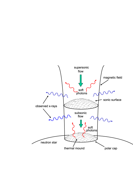
Figure 1: Schematic depiction of gas accreting onto the magnetic polar cap of a neutron star. Seed photons are created throughout the column via bremsstrahlung and cyclotron emission, and additional blackbody seed photons are emitted from the surface of the thermal mound, near the base of the column.

2.4 Thermal and Bulk Comptonization

The strong compression that occurs as the plasma crosses the radiative shock renders it an ideal site for the bulk Comptonization of seed photons produced via bremsstrahlung, cyclotron, or blackbody emission. In the bulk Comptonization process, particles experience a mean energy gain if the scattering centers they collide with are involved in a converging flow (e.g., Laurent & Titarchuk 1999; Turolla, Zane, & Titarchuk 2002). By contrast, in the thermal Comptonizaton process, particles gain energy due to the stochastic motions of the scattering centers via the second-order Fermi mechanism (e.g., Sunyaev & Titarchuk 1980; Becker 2003). In the X-ray pulsar application, the scattering centers are infalling electrons, and the energized “particles” are photons. Since the inflow speed of the electrons in an X-ray pulsar accretion column is much larger than their thermal velocity, bulk Comptonization dominates over the stochastic process except at the highest photon energies (Titarchuk, Mastichiadis, & Kylafis 1996).

The fundamental character of the Green’s function describing both thermal and bulk Comptonization was studied by Titarchuk & Zannias (1998) for the case of accretion onto a black hole. These authors established that the Green’s function can be approximated using a broken power-law form with a central peak between the high- and low-energy portions of the spectrum, for either type of Comptonization. Furthermore, they concluded that bulk Comptonization dominates over the thermal process if the electron temperature $T_{e}\lower 1.72218pt\hbox{$\;\buildrel<\over{\scriptstyle\sim}\;$}10^{7}\,$K. The theory developed in the present paper represents an extension of the same idea to neutron star accretion, resulting in the exact Green’s function for the X-ray pulsar spectral formation process. In agreement with Titarchuk & Zannias (1998), we find that the bulk Comptonization process dominates the energy exchange between the electrons and the photons for the temperature range relevant in X-ray pulsars. However, we also establish that thermal Comptonization nonetheless plays a central role in forming the characteristic spectral shapes noted in the bright sources. For example, Compton scattering of the high-energy photons is crucial for producing the observed quasi-exponential turnovers at high energies as a result of electron recoil, which is part of the thermal Comptonization process represented by the Kompaneets operator discussed in § 3. The subsequent inverse-Compton scattering of soft photons by the recoiling electrons redistributes the energy to lower frequency photons, helping to flatten the spectra as observed.

Lyubarskii & Sunyaev (1982) analyzed the effect of bulk and thermal Comptonization in the context of neutron star accretion using the same dynamical model for the flow considered here. However, they did not include the effect of photon escape from the accretion column, which renders their model inapplicable for the modeling of spectral formation in X-ray pulsars. In this paper we extend the work of Lyubarskii & Sunyaev by including the crucial effect of photon escape. Poutanen & Gierliński (2003) computed X-ray pulsar spectra based on the thermal Comptonization of soft radiation in a hot layer above the magnetic pole, but their model did not include a complete treatment of the bulk process, which is of central importance in X-ray pulsars. The new theory presented here therefore represents the first exact, quantitative analysis of the role of bulk and thermal Comptonization in the X-ray pulsar spectral formation process.

3 FORMATION OF THE RADIATION SPECTRUM

We follow the approach of Basko & Sunyaev (1975, 1976) and Becker & Wolff (2005b), and assume that the upstream flow is composed of pure, fully-ionized hydrogen moving at a highly supersonic speed, which is the standard scenario for accretion-powered X-ray pulsars. Our transport model employs a cylindrical, plane-parallel geometry, and therefore the velocity, density, and pressure are functions of the distance above the stellar surface, but they are all constant across the column at a given height (see Fig. 1). In the region above the thermal mound in a luminous X-ray pulsar, the gas is radiation-dominated, and the photons interact with the matter primarily via electron scattering, which controls both the spatial transport and the energization of the radiation (Arons et al. 1987). “Seed” photons injected into the flow are unable to diffuse very far up into the accreting gas due to the extremely high speed of the inflow. Most of the photons therefore escape through the walls of the column within a few scattering lengths of the mound, forming a “fan” type beam pattern, as expected for accretion-powered X-ray pulsars (e.g., Harding 1994, 2003). We are interested in obtaining the steady-state, polarization mode-averaged photon distribution function, $f(z,\epsilon)$, measured at altitude $z$ and energy $\epsilon$ inside the column resulting from the reprocessing of blackbody, cyclotron, and bremsstrahlung seed photons. The normalization of $f$ is defined so that $\epsilon^{2}f(z,\epsilon)\,d\epsilon$ gives the number density of photons in the energy range between $\epsilon$ and $\epsilon+d\epsilon$, and therefore $f$ is related to the occupation number distribution $\bar{n}$ via $f=8\pi\,\bar{n}/(c^{3}h^{3})$.

3.1 Transport Equation

In the cylindrical, plane-parallel geometry employed here, the photon distribution $f(z,\epsilon)$ satisfies the transport equation (e.g., Becker & Begelman 1986; Blandford & Payne 1981a; Becker 2003)

$${\partial f\over\partial t}+v\,{\partial f\over\partial z} = {dv\over dz}\,{\epsilon\over 3}\,{\partial f\over\partial\epsilon}+{\partial\over\partial z}\left({c\over 3n_{e}\sigma_{\|}}\,{\partial f\over\partial z}\right)-{f\over t_{\rm esc}}$$ (15)

$$+ {n_{e}\overline{\sigma}c\over m_{e}c^{2}}{1\over\epsilon^{2}}{\partial\over\partial\epsilon}\left[\epsilon^{4}\left(f+kT_{e}\,{\partial f\over\partial\epsilon}\right)\right]+{Q(z,\epsilon)\over\pi r_{0}^{2}}\ ,$$

where $z$ is the distance from the stellar surface along the column axis, $v<0$ is the inflow velocity, $Q$ denotes the photon source distribution, and $t_{\rm esc}$ represents the mean time photons spend in the plasma before diffusing through the walls of the column. The source function $Q$ is normalized so that $\epsilon^{2}\,Q(z,\epsilon)\,d\epsilon\,dz$ gives the number of seed photons injected per unit time between $z$ and $z+dz$ with energy between $\epsilon$ and $\epsilon+d\epsilon$. The left-hand side of equation (15) denotes the comoving time derivative of the radiation distribution $f$, and the terms on the right-hand side represent first-order Fermi energization (“bulk Comptonization”), spatial diffusion along the column axis, photon escape, thermal Comptonization, and photon injection, respectively. We are interested here in the steady-state version of equation (15) with $\partial f/\partial t=0$. The transport equation employed here is similar to the one analyzed by Becker & Wolff (2005b), except that thermal Comptonization has now been included via the appearance of the Kompaneets (1957) operator, and the source term $Q$ has been generalized to treat the production of seed radiation throughout the column, rather than focusing exclusively on the injection of blackbody photons at the surface of the thermal mound. Equation (15) does not include the term used by Becker & Wolff (2005b) to describe absorption at the thermal mound surface because this effect is negligible when bremsstrahlung and cyclotron emission are included in the model, as discussed in § 8. The total photon number and energy densities associated with the radiation distribution $f$ are given, respectively, by

$$n(z)=\int_{0}^{\infty}\epsilon^{2}\,f(z,\epsilon)\,d\epsilon\ ,\ \ \ \ U(z)=\int_{0}^{\infty}\epsilon^{3}\,f(z,\epsilon)\,d\epsilon\ .$$ (16)

Following Becker (1998) and Becker & Wolff (2005b), we compute the mean escape time using the diffusive prescription

$$t_{\rm esc}(z)={r_{0}\,\tau_{\perp}\over c}\ ,\ \ \ \ \ \tau_{\perp}(z)=n_{e}\,\sigma_{\perp}\,r_{0}\ ,$$ (17)

where $\tau_{\perp}$ represents the perpendicular scattering optical thickness of the cylindrical accretion column, and $\tau_{\perp}$ and $t_{\rm esc}$ are each functions of $z$ through their dependence on the electron number density $n_{e}$. Becker (1998) confirmed that the diffusion approximation employed in equation (17) is valid since $\tau_{\perp}>1$ for typical X-ray pulsar parameters. Equation (17) for the mean escape timescale can be rewritten as

$$t_{\rm esc}(z)={\dot{M}\,\sigma_{\perp}\over\pi m_{p}\,c\,|v|}\ ,$$ (18)

where

$$\dot{M}\equiv\pi r_{0}^{2}\,\rho\,|v|={\rm constant}\ ,$$ (19)

and $\rho=m_{p}\,n_{e}$. Since the escape timescale is inversely proportional to the flow velocity, the column becomes completely opaque at the surface of the neutron star due to the divergence of the electron number density there. The relationship between the escape-probability formalism employed here and the physical distribution of radiation inside the accretion column was discussed in detail by Becker & Wolff (2005b) in their § 6.3.

In our approach to solving equation (15) for the spectrum $f(z,\epsilon)$ inside the accretion column, we shall first obtain the Green’s function, $f_{{}_{\rm G}}(z_{0},z,\epsilon_{0},\epsilon)$, which is the radiation distribution at location $z$ and energy $\epsilon$ resulting from the injection of $\dot{N}_{0}$ photons per second with energy $\epsilon_{0}$ from a monochromatic source at location $z_{0}$. The determination of the Green’s function is a useful intermediate step in the process because it provides us with fundamental physical insight into the spectral redistribution process, and it also allows us to calculate the particular solution for the spectrum $f$ associated with an arbitrary photon source $Q(z,\epsilon)$ using the integral convolution (Becker 2003)

$$f(z,\epsilon)=\int_{0}^{\infty}\int_{0}^{\infty}{f_{{}_{\rm G}}(z_{0},z,\epsilon_{0},\epsilon)\over\dot{N}_{0}}\ \epsilon_{0}^{2}\,Q(z_{0},\epsilon_{0})\,d\epsilon_{0}\,dz_{0}\ .$$ (20)

The technical approach used to solve for the Green’s function, carried out in § 4, involves the derivation of eigenvalues and associated eigenfunctions based on the set of spatial boundary conditions for the problem (see, e.g., Blandford & Payne 1981b; Payne & Blandford 1981; Schneider & Kirk 1987; Colpi 1988).

The steady-state transport equation governing the Green’s function $f_{{}_{\rm G}}$ is (cf. eq. [15])

$$v\,{\partial f_{{}_{\rm G}}\over\partial z} = {dv\over dz}\,{\epsilon\over 3}\,{\partial f_{{}_{\rm G}}\over\partial\epsilon}+{\partial\over\partial z}\left({c\over 3n_{e}\sigma_{\|}}\,{\partial f_{{}_{\rm G}}\over\partial z}\right)-{f_{{}_{\rm G}}\over t_{\rm esc}}$$ (21)

$$+ {n_{e}\overline{\sigma}c\over m_{e}c^{2}}{1\over\epsilon^{2}}{\partial\over\partial\epsilon}\left[\epsilon^{4}\left(f_{{}_{\rm G}}+kT_{e}\,{\partial f_{{}_{\rm G}}\over\partial\epsilon}\right)\right]+{\dot{N}_{0}\,\delta(\epsilon-\epsilon_{0})\,\delta(z-z_{0})\over\pi r_{0}^{2}\epsilon_{0}^{2}}\ ,$$

and the associated radiation number and energy densities are given by (cf. eqs. [16])

$$n_{{}_{\rm G}}(z)\equiv\int_{0}^{\infty}\epsilon^{2}\,f_{{}_{\rm G}}(z_{0},z,\epsilon_{0},\epsilon)\,d\epsilon\ ,\ \ \ \ \ U_{{}_{\rm G}}(z)\equiv\int_{0}^{\infty}\epsilon^{3}\,f_{{}_{\rm G}}(z_{0},z,\epsilon_{0},\epsilon)\,d\epsilon\ .$$ (22)

Following Lyubarskii & Sunyaev (1982), we will assume that the electron temperature $T_{e}$ has a constant value, which is physically reasonable since most of the Comptonization occurs in a relatively compact region above the thermal mound. However, it is important to confirm the validity of this assumpton using a detailed numerical model that incorporates a self-consistent calculation of the temperature distribution, which we plan to develop in future work. Under the assumption of a constant electron temperature, it is convenient to work in terms of the dimensionless energy variable $\chi$, defined by

$$\chi(\epsilon)\equiv{\epsilon\over kT_{e}}\ .$$ (23)

We can make further progress by transforming the spatial variable from $z$ to the scattering optical depth parallel to the magnetic field, $\tau$, which is related to $z$ via

$$d\tau=n_{e}(z)\,\sigma_{\|}\,dz\ ,\ \ \ \ \tau(z)=\int_{0}^{z}n_{e}(z^{\prime})\,\sigma_{\|}\,dz^{\prime}\ ,$$ (24)

so that $z$ and $\tau$ both vanish at the stellar surface.

Making the change of variable from $z$ to $\tau$ in equation (21), we find after some algebra that the transport equation for the Green’s function can be written in the form

$${v\over c}\,{\partial f_{{}_{\rm G}}\over\partial\tau} = {1\over c}\,{dv\over d\tau}\,{\chi\over 3}\,{\partial f_{{}_{\rm G}}\over\partial\chi}+{1\over 3}\,{\partial^{2}f_{{}_{\rm G}}\over\partial\tau^{2}}-{\xi^{2}\,v^{2}\over c^{2}}\,f_{{}_{\rm G}}$$ (25)

$$+ {\overline{\sigma}\over\sigma_{\|}}\,{kT_{e}\over m_{e}c^{2}}{1\over\chi^{2}}{\partial\over\partial\chi}\left[\chi^{4}\left(f_{{}_{\rm G}}+{\partial f_{{}_{\rm G}}\over\partial\chi}\right)\right]+{\dot{N}_{0}\,\delta(\chi-\chi_{0})\,\delta(\tau-\tau_{0})\over\pi r_{0}^{2}ckT_{e}\epsilon_{0}^{2}}\ ,$$

where $\tau_{0}\equiv\tau(z_{0})$, $\chi_{0}\equiv\chi(\epsilon_{0})$, and we have introduced the dimensionless parameter

$$\xi\equiv{\pi r_{0}m_{p}c\over\dot{M}(\sigma_{\|}\sigma_{\perp})^{1/2}}\ ,$$ (26)

which determines the importance of the escape of photons from the accretion column. Becker (1998) derived the exact solution for the flow velocity profile in a radiation-dominated pulsar accretion column, and demonstrated that the condition $\xi=2/\sqrt{3}$ must be satisfied in order to ensure that the flow comes to rest at the stellar surface. This condition represents a balance between the characteristic timescale for photon escape and the dynamical (accretion) timescale, as discussed in § 6. Physically, this balance reflects the requirement that the kinetic energy of the flow must be radiated away through the column walls in the same amount of time required for the gas to settle onto the star. Note that we can write the Green’s function as either $f_{{}_{\rm G}}(z_{0},z,\epsilon_{0},\epsilon)$ or $f_{{}_{\rm G}}(\tau_{0},\tau,\chi_{0},\chi)$ since the variables $(z,\epsilon)$ and $(\chi,\tau)$ are interchangeable via equations (23) and (24).

3.2 Separability

Lyubarskii & Sunyaev (1982) demonstrated that when $\chi\neq\chi_{0}$, the transport equation (25) is separable in energy and space if the velocity profile has the particular form

$$v(\tau)=-\alpha\,c\,\tau\ ,$$ (27)

where $\alpha$ is a positive constant. By combining equations (19), (24), (26), and (27), we can express $\tau$ as an explicit function of the altitude $z$, obtaining

$$\tau(z)=\left(\sigma_{\|}\over\sigma_{\perp}\right)^{1/4}\left(2\,z\over\alpha\,\xi\,r_{0}\right)^{1/2}\ .$$ (28)

Using this result to substitute for $\tau$ in equation (27), we note that the velocity profile required for separability is related to $z$ via

$$v(z)=-\left(\sigma_{\|}\over\sigma_{\perp}\right)^{1/4}\left(2\,\alpha z\over\xi\,r_{0}\right)^{1/2}c\ .$$ (29)

Although this profile describes a flow that stagnates at the stellar surface ($\tau=0$, $z=0$) as required, the details of the velocity variation deviate somewhat from the exact solution for the velocity profile in a radiation-dominated pulsar accretion column derived by Becker (1998) and Basko & Sunyaev (1976), which can be stated in terms of the altitude $z$ using

$$v_{\rm ex}(z)=-v_{\rm ff}\left[1-\left(7\over 3\right)^{-z/z_{\rm sp}}\right]\ ,$$ (30)

where the free-fall velocity from infinity onto the stellar surface, $v_{\rm ff}$, and the altitude at the sonic point, $z_{\rm sp}$, are given by

$$v_{\rm ff}\equiv\left(2\,GM_{*}\over R_{*}\right)^{1/2}\ ,\ \ \ \ z_{\rm sp}\equiv{r_{0}\over 2\sqrt{3}}\left(\sigma_{\perp}\over\sigma_{\|}\right)^{1/2}\ln\left(7\over 3\right)\ .$$ (31)

In order to make further mathematical progress in the computation of the radiation spectrum emitted by the accretion column, we must utilize the approximate (separable) velocity profile given by equation (29). However, before doing so, we must ensure that the approximate velocity profile agrees reasonably well with the exact profile (eq. [30]) in the lower portion of the accretion column, where most of the spectral formation occurs. We can accomplish this by setting the two profiles equal to each other at the sonic point ($z=z_{\rm sp}$), and using this condition to solve for the constant $\alpha$, which yields

$$\alpha={32\,\sqrt{3}\over 49\,\ln(7/3)}\ {GM_{*}\,\xi\over R_{*}\,c^{2}}\ ,$$ (32)

or, equivalently,

$$\alpha=0.20\left(M_{*}\over M_{\odot}\right)\left(R_{*}\over 10\,{\rm km}\right)^{-1}\xi\ .$$ (33)

This relation allows us to compute $\alpha$ as a function of $\xi$ for given values of the stellar mass $M_{*}$ and radius $R_{*}$. In radiation-dominated pulsar accretion columns, $\xi=2/\sqrt{3}$, and therefore $\alpha$ is of order unity (Becker 1998).

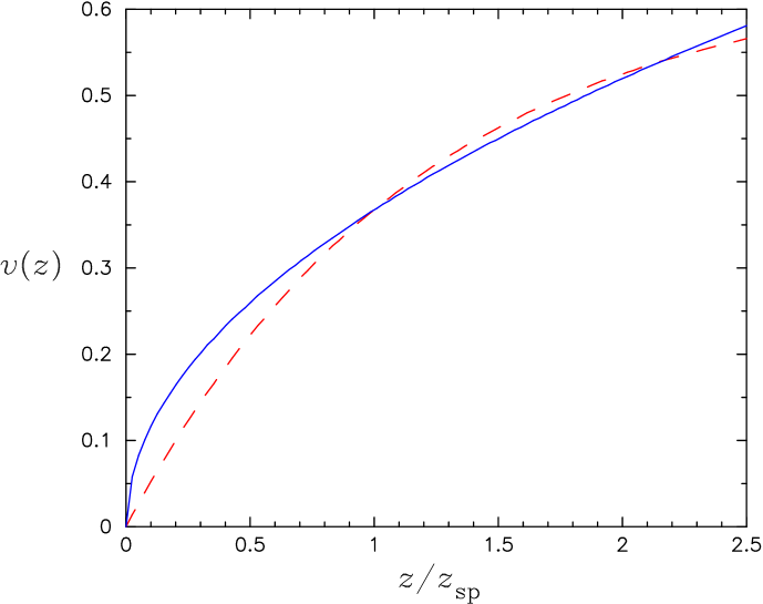
Figure 2: Comparison of the approximate (solid line) and exact (dashed line) velocity profiles evaluated using eqs. (29) and (30), respectively, in units of $c$. The constant $\alpha$ has been computed using eq. (32), which ensures that the two velocities agree at the sonic point, $z=z_{\rm sp}$.

The detailed shapes of the approximate (eq. [29]) and exact (eq. [30]) velocity profiles as functions of $z$ are compared in Figure 2. In general, the two functions agree fairly well, although the approximate profile overestimates the correct velocity close to the stellar surface. Nevertheless, since the overall compression associated with the approximate profile is correct, we expect that the net effect of bulk Comptonization will be accurately modeled using the approximate profile. We will therefore adopt the form for the velocity profile given in terms of $\tau$ by equation (27) or in terms of $z$ by equation (29), with $\alpha$ computed using equation (33). The validity of this approach will be carefully examined in § 6 by comparing the results obtained for the Comptonization of radiation in a “cold” accretion flow ($T_{e}\to 0$) described by the approximate velocity profile with those computed using the model of Becker & Wolff (2005b), who treated the Comptonization of radiation in a cold accretion column, described by the exact velocity profile.

4 EXACT SOLUTION FOR THE GREEN’S FUNCTION

Adopting the velocity profile given by equation (27), we find that the transport equation (25) for the Green’s function can be reorganized to obtain

$${\alpha\,\chi\over 3}\,{\partial f_{{}_{\rm G}}\over\partial\chi}-{\overline{\sigma}\over\sigma_{\|}}\,{kT_{e}\over m_{e}c^{2}}{1\over\chi^{2}}{\partial\over\partial\chi}\left[\chi^{4}\left(f_{{}_{\rm G}}+{\partial f_{{}_{\rm G}}\over\partial\chi}\right)\right] = {1\over 3}\,{\partial^{2}f_{{}_{\rm G}}\over\partial\tau^{2}}+\alpha\,\tau\,{\partial f_{{}_{\rm G}}\over\partial\tau}-\xi^{2}\alpha^{2}\,\tau^{2}\,f_{{}_{\rm G}}$$ (34)

$$+ {\dot{N}_{0}\,\delta(\chi-\chi_{0})\,\delta(\tau-\tau_{0})\over\pi r_{0}^{2}ckT_{e}\epsilon_{0}^{2}}\ .$$

Lyubarskii & Sunyaev (1982) analyzed this equation for the special case $\xi=0$, which corresponds to the neglect of the escape of photons from the accretion column. Their results do not describe the formation of the emergent spectrum in an accretion-powered X-ray pulsar since photon escape is a critical part of that process. We therefore extend the results of Lyubarskii & Sunyaev below by deriving the closed-form solution for the Green’s function in the X-ray pulsar problem for the general case with $\xi>0$.

When $\chi\neq\chi_{0}$, the $\delta$-function in the transport equation (34) makes no contribution, and therefore the differential equation is linear and homogeneous. The transport equation can then be separated in energy and space using the functions

$$f_{\lambda}(\tau,\chi)\equiv g(\lambda,\tau)\ h(\lambda,\chi)\ ,$$ (35)

where $\lambda$ is the separation constant. We find that the spatial and energy functions, $g$ and $h$, respectively, satisfy the differential equations

$${1\over 3}\,{d^{2}g\over d\tau^{2}}+\alpha\,\tau\,{dg\over d\tau}+\left({\alpha\lambda\over 3}-\xi^{2}\alpha^{2}\tau^{2}\right)g=0\ ,$$ (36)

and

$${1\over\chi^{2}}{d\over d\chi}\left[\chi^{4}\left(h+{dh\over d\chi}\right)\right]-\delta\,\chi\,{dh\over d\chi}-\delta\,\lambda\,h=0\ ,$$ (37)

where the parameter $\delta$ is defined by

$$\delta\equiv{\alpha\over 3}\,{\sigma_{\|}\over\overline{\sigma}}\,{m_{e}c^{2}\over kT_{e}}\ .$$ (38)

This is equivalent to the quantity $\delta$ introduced by Lyubarskii & Sunyaev (1982) if we set $\overline{\sigma}=\sigma_{\|}$, since these authors did not include any angle dependence in the electron scattering cross section.

4.1 Eigenvalues and Spatial Eigenfunctions

In order to obtain the solution for the spatial separation function $g$, we must first consider the boundary conditions that $g$ must satisfy. In the downstream region, as the gas approaches the stellar surface, we expect the advective and diffusive components of the radiation flux to vanish due to the divergence of the electron density. The advective flux is indeed negligible at the stellar surface since $v\to 0$ as $\tau\to 0$ (see eq. [27]). However, in order to ensure that the diffusive flux vanishes, we must require that $dg/d\tau\to 0$ as $\tau\to 0$. Conversely, in the upstream region, we expect that $g\to 0$ as $\tau\to\infty$ since no photons can diffuse to large distances in the direction opposing the plasma flow. With these boundary conditions taken into consideration, we find that the fundamental solution for the spatial separation function $g$ has the general form

$$g(\lambda,\tau)\propto\cases{e^{-\alpha(3+w)\tau^{2}/4}\,M\left(a,{1\over 2},{\alpha w\tau^{2}\over 2}\right)\ ,&$\tau\leq\tau_{0}$ \ ,\cr e^{-\alpha(3+w)\tau^{2}/4}\,U\left(a,{1\over 2},{\alpha w\tau^{2}\over 2}\right)\ ,&$\tau\geq\tau_{0}$ \ ,\cr}$$ (39)

where $M$ and $U$ denote confluent hypergeometric functions (Abramowitz & Stegun 1970), and we have made the definitions

$$a\equiv{w+3-2\lambda\over 4w}\ ,\ \ \ \ \ w\equiv\left(9+12\,\xi^{2}\right)^{1/2}\ .$$ (40)

Note that in the radiation-dominated case with $\xi=2/\sqrt{3}$, we obtain $w=5$.

Equation (36) is linear, second-order, and homogeneous, and consequently both the function $g$ and its derivative $dg/d\tau$ must be continuous at the source location, $\tau=\tau_{0}$. The smooth merger of the $M$ and $U$ functions at the source location requires that their Wronskian,

$$\omega(\tau) \equiv M\left(a,{1\over 2},{\alpha w\tau^{2}\over 2}\right){d\over d\tau}\,U\left(a,{1\over 2},{\alpha w\tau^{2}\over 2}\right)$$ (41)

$$- \ U\left(a,{1\over 2},{\alpha w\tau^{2}\over 2}\right){d\over d\tau}\,M\left(a,{1\over 2},{\alpha w\tau^{2}\over 2}\right)\ ,$$

must vanish at $\tau=\tau_{0}$. This condition can be used to solve for the eigenvalues of the separation constant $\lambda$. By employing equation (13.1.22) from Abramowitz & Stegun (1970) to evaluate the Wronskian, we obtain the eigenvalue equation

$$\omega(\tau)=-{\Gamma(1/2)\,(2\alpha w)^{1/2}\over\Gamma(a)}\ e^{\alpha w\tau^{2}/2}=0\ .$$ (42)

The left-hand side vanishes when $\Gamma(a)\to\pm\infty$, which implies that $a=-n$, where $n=0,1,2,$…By combining this result with equation (40), we conclude that the eigenvalues $\lambda_{n}$ are given by

$$\lambda_{n}={4nw+w+3\over 2}\ ,\ \ \ \ n=0,1,2,\ldots$$ (43)

When $\lambda=\lambda_{n}$, the spatial separation functions $g$ reduce to a set of global eigenfunctions that satisfy the boundary conditions at large and small values of $\tau$. In this case, we can use equations (13.6.9) and (13.6.27) from Abramowitz & Stegun to show that the confluent hypergeometric functions $M$ and $U$ appearing in equation (41) are proportional to the generalized Laguerre polynomials $L_{n}^{(-1/2)}$, and consequently the spatial eigenfunctions can be written as

$$g_{n}(\tau)\equiv g(\lambda_{n},\tau)=e^{-\alpha(3+w)\tau^{2}/4}\,L_{n}^{(-1/2)}\left(\alpha w\tau^{2}\over 2\right)\ .$$ (44)

Based on equation (7.414.3) from Gradshteyn & Ryzhik (1980), we note that the spatial eigenfunctions satisfy the orthogonality relation

$$\int_{0}^{\infty}e^{3\alpha\tau^{2}/2}g_{n}(\tau)\,g_{m}(\tau)\,d\tau=\cases{{\Gamma(n+1/2)\over n!\,\sqrt{2\alpha w}}\ ,&$n=m$ \ ,\cr 0\ ,&$n\neq m$ \ .\cr}$$ (45)

4.2 Energy Eigenfunctions

The solution for the energy separation function $h$ depends on the boundary conditions imposed in the energy space. As $\epsilon\to 0$, we require that $h$ not increase faster than $\epsilon^{-3}$ since the Green’s function must possess a finite total photon number density (see eq. [22]). Conversely, as $\epsilon\to\infty$, we require that $h$ decrease more rapidly than $\epsilon^{-4}$ in order to ensure that the Green’s function contains a finite total photon energy density. Furthermore, in order to avoid an infinite diffusive flux in the energy space at $\chi=\chi_{0}$, the function $h$ must be continuous there. The fundamental solution for the energy eigenfunction that satisfies the various boundary and continuity conditions can be written as

$$h_{n}(\chi)\equiv h(\lambda_{n},\chi)=\cases{\chi^{\kappa-4}\,e^{-\chi/2}\,W_{\kappa,\mu}(\chi_{0})\,M_{\kappa,\mu}(\chi)\ ,&$\chi\leq\chi_{0}$ \ ,\cr\chi^{\kappa-4}\,e^{-\chi/2}\,M_{\kappa,\mu}(\chi_{0})\,W_{\kappa,\mu}(\chi)\ ,&$\chi\geq\chi_{0}$ \ ,\cr}$$ (46)

where $M_{\kappa,\mu}$ and $W_{\kappa,\mu}$ denote Whittaker functions, and we have made the definitions

$$\kappa\equiv{1\over 2}\,(\delta+4)\ ,\ \ \ \ \ \mu\equiv{1\over 2}\left[(3-\delta)^{2}+4\,\delta\lambda_{n}\right]^{1/2}\ .$$ (47)

Note that each of the eigenvalues $\lambda_{n}$ results in a different value for $\mu$, and the parameter $\delta$ is defined in equation (38). Equation (46) can also be written in the more compact form

$$h_{n}(\chi)=\chi^{\kappa-4}\,e^{-\chi/2}\,M_{\kappa,\mu}(\chi_{\rm min})\,W_{\kappa,\mu}(\chi_{\rm max})\ ,$$ (48)

where

$$\chi_{\rm min}\equiv\min(\chi,\chi_{0})\ ,\ \ \ \ \ \chi_{\rm max}\equiv\max(\chi,\chi_{0})\ .$$ (49)

4.3 Eigenfunction Expansion

The spatial eigenfunctions $g_{n}(y)$ form an orthogonal set, as expected since this is a standard Sturm-Liouville problem. The solution for the Green’s function can therefore be expressed as the infinite series

$$f_{{}_{\rm G}}(\tau_{0},\tau,\chi_{0},\chi)=\sum_{n=0}^{\infty}\ C_{n}\,g_{n}(\tau)\,h_{n}(\chi)\ ,$$ (50)

where the expansion coefficients $C_{n}$ are computed by employing the orthogonality of the eigenfunctions, along with the derivative jump condition

$$\lim_{\varepsilon\to 0}\ {\partial f_{{}_{\rm G}}\over\partial\chi}\Bigg{|}_{\chi=\chi_{0}+\varepsilon}-{\partial f_{{}_{\rm G}}\over\partial\chi}\Bigg{|}_{\chi=\chi_{0}-\varepsilon}=-\,{3\dot{N}_{0}\,\delta\,kT_{e}\,\delta(\tau-\tau_{0})\over\alpha\,\pi r_{0}^{2}\,c\,\epsilon_{0}^{4}}\ ,$$ (51)

which is obtained by integrating the transport equation (34) with respect to $\chi$ in a very small range surrounding the injection energy $\chi_{0}$. Substituting using the expansion for $f_{{}_{\rm G}}$ yields

$$\lim_{\varepsilon\to 0}\ \sum_{n=0}^{\infty}\ C_{n}\,g_{n}(\tau)\,\left[h_{n}^{\prime}(\chi_{0}+\varepsilon)-h_{n}^{\prime}(\chi_{0}-\varepsilon)\right]=-\,{3\dot{N}_{0}\,\delta\,kT_{e}\,\delta(\tau-\tau_{0})\over\alpha\,\pi r_{0}^{2}\,c\,\epsilon_{0}^{4}}\ ,$$ (52)

where primes denote differentiation with respect to $\chi$. By employing equation (48) for $h_{n}$, we find that

$$\sum_{n=0}^{\infty}\ C_{n}\,g_{n}(\tau)\,\chi_{0}^{\kappa-4}\,e^{-\chi_{0}/2}\mathfrak{W}(\chi_{0})=-\,{3\dot{N}_{0}\,\delta\,kT_{e}\,\delta(\tau-\tau_{0})\over\alpha\,\pi r_{0}^{2}\,c\,\epsilon_{0}^{4}}\ ,$$ (53)

where the Wronskian, $\mathfrak{W}$, is defined by

$$\mathfrak{W}(\chi_{0})\equiv M_{\kappa,\mu}(\chi_{0})\,W^{\prime}_{\kappa,\mu}(\chi_{0})-W_{\kappa,\mu}(\chi_{0})\,M^{\prime}_{\kappa,\mu}(\chi_{0})\ .$$ (54)

The Wronskian can be evaluated analytically using equations (13.1.22), (13.1.32), and (13.1.33) from Abramowitz & Stegun (1970), which yields

$$\mathfrak{W}(\chi_{0})=-\,{\Gamma(1+2\mu)\over\Gamma(\mu-\kappa+1/2)}\ .$$ (55)

Using this result to substitute for $\mathfrak{W}(\chi_{0})$ in equation (53) and reorganizing the terms, we obtain

$$\sum_{n=0}^{\infty}\ {\Gamma(1+2\mu)\,C_{n}\,g_{n}(\tau)\over\Gamma(\mu-\kappa+1/2)}={3\dot{N}_{0}\,\delta\,e^{\chi_{0}/2}\,\delta(\tau-\tau_{0})\over\alpha\,\pi r_{0}^{2}\,c\,\chi_{0}^{\kappa}\,(kT_{e})^{3}}\ ,$$ (56)

where $\mu$ is a function of $\lambda_{n}$ via equation (47). We can now calculate the expansion coefficients $C_{n}$ by utilizing the orthogonality of the spatial eigenfunctions $g_{n}$ represented by equation (45). Multiplying both sides of equation (56) by $e^{3\alpha\tau^{2}/2}g_{m}(\tau)$ and integrating with respect to $\tau$ from zero to infinity yields, after some algebra,

$$C_{n}={3\dot{N}_{0}\,\delta\,\sqrt{2w}\ e^{\chi_{0}/2}\,e^{3\alpha\tau_{0}^{2}/2}\over\pi r_{0}^{2}\,c(kT_{e})^{3}\chi_{0}^{\kappa}\,\sqrt{\alpha}}\,{\Gamma(\mu-\kappa+1/2)\ n!\,g_{n}(\tau_{0})\over\Gamma(1+2\mu)\,\Gamma(n+1/2)}\ .$$ (57)

The final closed-form solution for the Green’s function, obtained by combining equations (48), (50), and (57), is given by

$$f_{{}_{\rm G}}(\tau_{0},\tau,\chi_{0},\chi) = {3\dot{N}_{0}\,\delta\,e^{3\alpha\tau_{0}^{2}/2}\sqrt{2w}\ \chi^{\kappa-4}\,e^{(\chi_{0}-\chi)/2}\over\pi r_{0}^{2}\,c(kT_{e})^{3}\chi_{0}^{\kappa}\sqrt{\alpha}}\sum_{n=0}^{\infty}\ {\Gamma(\mu-\kappa+1/2)\,n!\over\Gamma(1+2\mu)\,\Gamma(n+1/2)}$$ (58)

$$\times g_{n}(\tau_{0})\,g_{n}(\tau)\,M_{\kappa,\mu}(\chi_{\rm min})\,W_{\kappa,\mu}(\chi_{\rm max})\ ,$$

where the spatial eigenfunctions $g_{n}$ are computed using equation (44) and the parameters $\kappa$ and $\mu$ are given by equations (47). The Green’s function can also be expressed directly in terms of the photon energy $\epsilon$ by writing

$$f_{{}_{\rm G}}(\tau_{0},\tau,\epsilon_{0},\epsilon) = {3\dot{N}_{0}\,\delta\,kT_{e}\,e^{3\alpha\tau_{0}^{2}/2}\sqrt{2w}\ \epsilon^{\kappa-4}\,e^{(\epsilon_{0}-\epsilon)/(2kT_{e})}\over\pi r_{0}^{2}\,c\,\epsilon_{0}^{\kappa}\sqrt{\alpha}}\sum_{n=0}^{\infty}\ {\Gamma(\mu-\kappa+1/2)\,n!\over\Gamma(1+2\mu)\,\Gamma(n+1/2)}$$ (59)

$$\times g_{n}(\tau_{0})\,g_{n}(\tau)\,M_{\kappa,\mu}\left(\epsilon_{\rm min}\over kT_{e}\right)W_{\kappa,\mu}\left(\epsilon_{\rm max}\over kT_{e}\right)\ ,$$

where

$$\epsilon_{\rm min}\equiv\min(\epsilon,\epsilon_{0})\ ,\ \ \ \ \ \epsilon_{\rm max}\equiv\max(\epsilon,\epsilon_{0})\ .$$ (60)

This exact, analytical solution for $f_{{}_{\rm G}}$ is one of the main results of the paper, and it provides a very efficient means for computing the steady-state Green’s function resulting from the continual injection of monochromatic seed photons from a source at an arbitrary location inside the accretion column. The eigenfunction expansion converges rapidly and therefore we can generally obtain an accuracy of at least four significant figures in our calculations of $f_{{}_{\rm G}}$ by terminating the series in equations (58) or (59) after the first 5-10 terms.

4.4 Asymptotic Power-Law Behavior

Asymptotic analysis of the energy function $W_{\kappa,\mu}$ appearing in equation (59) reveals that if the photon energy $\epsilon$ and injection energy $\epsilon_{0}$ satisfy the conditions $\epsilon_{0}<\epsilon\ll kT_{e}$, then the spectrum has the power-law form

$$f_{{}_{\rm G}}\propto\epsilon^{-[3-\delta+\sqrt{(3-\delta)^{2}+4\lambda_{0}\delta}]/2}\ ,\ \ \ \ \ \lambda_{0}={w+3\over 2}\ ,$$ (61)

where $\delta$ is given by equation (38) and $\lambda_{0}$ is the leading eigenvalue computed using equation (43) with $n=0$. We will demonstrate in § 6 that bulk Comptonization dominates over thermal Comptonization in the limit of large $\delta$, in which case equation (61) reduces to

$$f_{{}_{\rm G}}\propto\epsilon^{-\lambda_{0}}\ ,\ \ \ \ \ \delta\to\infty\ ,$$ (62)

which is the same solution obtained by Becker & Wolff (2005b) in the case of pure bulk Comptonization. However, in contrast to the pure-bulk model, in the scenario considered here the power-law shape only extends up to the Wien turnover at photon energy $\epsilon\sim kT_{e}$.

We can gain some insight into the role of thermal Comptonization by comparing the power-law indices in equations (61) and (62). In general, we find that

$$\lambda_{0}\ \geq\ {3-\delta+\sqrt{(3-\delta)^{2}+4\lambda_{0}\delta}\over 2}\ ,$$ (63)

with the equality holding in the limit of large $\delta$. This implies that for small values of $\delta$, thermal Comptonization causes a flattening of the spectrum in the region $\epsilon\ll kT_{e}$ due to the transfer of energy from high- to medium-energy photons via electron recoil. If the flow is radiation-dominated, as expected in the bright pulsars, then $\xi=2/\sqrt{3}$ and we obtain $w=5$ and $\lambda_{0}=4$ according to equations (40) and (61), respectively. Luminous pulsars are generally dominated by bulk Comptonization, and therefore it follows that the photon spectral index $\alpha_{\rm X}\equiv\lambda_{0}-2=2$ in the region of the spectrum below the Wien cutoff.

5 SPECTRUM OF THE ESCAPING RADIATION

Equations (58) and (59) represent the exact solution for the Green’s function $f_{{}_{\rm G}}$ describing the radiation spectrum inside a pulsar accretion column resulting from the injection of $\dot{N}_{0}$ seed photons per unit time from a monochromatic source located at $\tau=\tau_{0}$ (or, equivalently, at $z=z_{0}$). Since the fundamental transport equation (15) is linear, we can use the analytical solutions for the Green’s function to calculate the spectrum of the radiation escaping from the accretion column for any desired source distribution.

5.1 Green’s Function for the Escaping Radiation Spectrum

In the escape-probability approach employed here, the associated Green’s function for the number spectrum of the photons escaping through the walls of the cylindrical column is computed using

$$\dot{N}_{\epsilon}^{\rm G}(z_{0},z,\epsilon_{0},\epsilon)\equiv{\pi\,r_{0}^{2}\,\epsilon^{2}\over t_{\rm esc}(z)}\,f_{{}_{\rm G}}(z_{0},z,\epsilon_{0},\epsilon)\ ,$$ (64)

where the escape timescale $t_{\rm esc}$ is evaluated as a function of $z$ by combining equations (18) and (29), which yields

$$t_{\rm esc}(z)=\left(\dot{M}\,\sigma_{\perp}^{2}\,r_{0}^{2}\over 2\pi\,m_{p}\,c^{3}\,\sigma_{\|}\,\alpha\,z\right)^{1/2}\ .$$ (65)

The quantity $\dot{N}_{\epsilon}^{\rm G}\,dz\,d\epsilon$ represents the number of photons emitted from the disk-shaped volume between positions $z$ and $z+dz$ per unit time with energy between $\epsilon$ and $\epsilon+d\epsilon$.

Since the quantities $(z,z_{0})$ and $(\tau,\tau_{0})$ are interchangeable via equations (24), we are free to work in terms of the more convenient parameters $(\tau,\tau_{0})$ without loss of generality. In this case equations (26), (28), and (65) can be combined to reexpress the escape timescale as

$$t_{\rm esc}(\tau)={r_{0}\over\alpha\,\xi\,c\,\tau}\left(\sigma_{\perp}\over\sigma_{\|}\right)^{1/2}\ .$$ (66)

By using this result to substitute for $t_{\rm esc}$ in equation (64), we find that the Green’s function for the escaping radiation spectrum is given in terms of the optical depth by

$$\dot{N}_{\epsilon}^{\rm G}(\tau_{0},\tau,\epsilon_{0},\epsilon)=\pi r_{0}\,c\,\alpha\,\xi\left(\sigma_{\|}\over\sigma_{\perp}\right)^{1/2}\tau\,\epsilon^{2}\,f_{{}_{\rm G}}(\tau_{0},\tau,\epsilon_{0},\epsilon)\ ,$$ (67)

where $f_{{}_{\rm G}}$ is computed using equation (59). The factor of $\tau$ on the right-hand side of equation (67) indicates that the emitted radiation is strongly attenuated near the stellar surface due to the divergence of the electron number density, which inhibits the escape of the photons through the walls of the accretion column. Equations (59) and (67) can be combined to express the closed-form solution for $\dot{N}_{\epsilon}^{\rm G}$ as

$$\dot{N}_{\epsilon}^{\rm G}(\tau_{0},\tau,\epsilon_{0},\epsilon)={3\dot{N}_{0}\,\delta\,\xi\,kT_{e}\,\sqrt{2\alpha w\sigma_{\|}}\ e^{3\alpha\tau_{0}^{2}/2}\epsilon^{\kappa-2}\,e^{(\epsilon_{0}-\epsilon)/(2kT_{e})}\,\tau\over r_{0}\,\epsilon_{0}^{\kappa}\,\sqrt{\sigma_{\perp}}}$$ (68)

$$\qquad\times\sum_{n=0}^{\infty}\ {\Gamma(\mu-\kappa+1/2)\,n!\over\Gamma(1+2\mu)\,\Gamma(n+1/2)}\ g_{n}(\tau_{0})\,g_{n}(\tau)\,M_{\kappa,\mu}\left(\epsilon_{\rm min}\over kT_{e}\right)W_{\kappa,\mu}\left(\epsilon_{\rm max}\over kT_{e}\right)\ ,$$

where $\epsilon_{\rm min}$ and $\epsilon_{\rm max}$ are defined by equations (60), and $w$, $\kappa$, and $\mu$ are computed using equations (40) and (47).

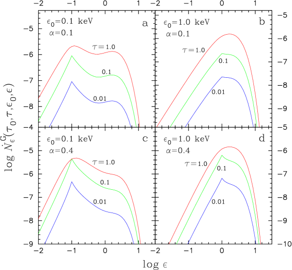
Figure 3: Green’s function $\dot{N}_{\epsilon}^{\rm G}$ ($\rm s^{-1}\,cm^{-1}\,keV^{-1}$) describing the photon number spectrum escaping from an X-ray pulsar accretion column as a function of the radiation energy $\epsilon$ (keV) and the scattering optical depth $\tau$ above the surface, evaluated using eq. (68). The curves were computed by setting $\sigma_{\|}=10^{-3}\,\sigma_{{}_{\rm T}}$, $\sigma_{\perp}=\sigma_{{}_{\rm T}}$, $\overline{\sigma}=0.1\,\sigma_{{}_{\rm T}}$, $\dot{N}_{0}=1$, $\xi=2/\sqrt{3}$, $\tau_{0}=0.1$, $r_{0}=10^{4}\,$cm, and $T_{e}=10^{7}\,$K. The values of $\tau$, $\epsilon_{0}$, and $\alpha$ are indicated for each plot, and the values of $\delta$ are discussed in the text.

In Figure 3 we plot the Green’s function for the escaping photon number distribution, $\dot{N}_{\epsilon}^{\rm G}$, as a function of the photon energy $\epsilon$ and the scattering optical depth $\tau$ above the stellar surface for two values of the parameters $\alpha$ and $\epsilon_{0}$ using equation (68). In order to clearly illustrate the general features of the spectrum, we set $\sigma_{\|}=10^{-3}\,\sigma_{{}_{\rm T}}$, $\sigma_{\perp}=\sigma_{{}_{\rm T}}$, $\overline{\sigma}=0.1\,\sigma_{{}_{\rm T}}$, $\dot{N}_{0}=1$, $\xi=2/\sqrt{3}$, $\tau_{0}=0.1$, $r_{0}=10^{4}\,$cm, and $T_{e}=10^{7}\,$K. We show in § 6 that the parameter $\delta$ defined by equation (38) determines the relative importance of bulk and thermal Comptonization. The values of $\delta$ obtained in Figure 3 are $\delta=0.20$ for $\alpha=0.1$, and $\delta=0.79$ for $\alpha=0.4$. For the cases with $\epsilon_{0}=0.1\,$keV, a distinct Wien hump is visible at $\epsilon\sim 1\,$keV due to thermal Comptonization. However, the hump is less pronounced when $\alpha=0.4$ due to the greater strength of bulk Comptonization, which tends to create a power-law spectral shape with photon index $\alpha_{\rm X}=2$ (see § 4.4). The Wien feature is almost invisible when $\epsilon_{0}=1\,$keV because in this case the energy of the injected photons is comparable to the thermal energy of the electrons. Note that for small values of $\tau$, the escape of radiation is inhibited because of the divergence of the electron density near the stellar surface. Little radiation is able to escape from the column for $\tau\gg 1$ because the photons are advectively trapped near the stellar surface due to the high-speed inflow (see § 6). Hence the spatial distribution of the escaping radiation peaks around $\tau\sim 1$.

5.2 Altitude-Dependent Spectrum for an Arbitrary Source

Since the fundamental transport equation (15) is linear, the analytical results for the Green’s function obtained in § 5.1 provide the basis for the consideration of any source distribution. By analogy with equation (64), we can compute the photon spectrum emitted through the walls of the accretion column for an arbitrary source distribution $Q$ in equation (15) by writing

$$\dot{N}_{\epsilon}(z,\epsilon)\equiv{\pi\,r_{0}^{2}\,\epsilon^{2}\over t_{\rm esc}(z)}\,f(z,\epsilon)\ ,$$ (69)

where $f$ is the particular solution calculated using the integral convolution given by equation (20). Substituting for $f_{{}_{\rm G}}$ and $f$ in equation (20) using equations (64) and (69), respectively, we find that the particular solution for the emitted photon spectrum can be written as

$$\dot{N}_{\epsilon}(z,\epsilon)=\int_{0}^{\infty}\int_{0}^{\infty}{\dot{N}_{\epsilon}^{\rm G}(z_{0},z,\epsilon_{0},\epsilon)\over\dot{N}_{0}}\ \epsilon_{0}^{2}\,Q(z_{0},\epsilon_{0})\,d\epsilon_{0}\,dz_{0}\ .$$ (70)

The spatial integration converges despite the infinite upper bound for $z_{0}$ because the seed photon distribution $Q$ is localized in the lower region of the accretion column (see § 6.1). Equation (70) facilitates the calculation of the photon spectrum emitted by the accretion column as a function of photon energy $\epsilon$ and altitude $z$ for any source distribution $Q$. However, due to the large distances to the known pulsars, current observations are unable to resolve the spatial distribution of the emission from the column. It is therefore necessary to integrate the emitted radiation field with respect to $z$ in order to compare the theoretical predictions with the available spectral data, as we discuss below.

5.3 Column-Integrated Escaping Green’s Function

By integrating over the vertical structure of the accretion column, we can compute the total emitted radiation distribution, which corresponds approximately to the phase-averaged spectrum of the X-ray pulsar. In the cylindrical geometry employed here, the formal integration domain is the region $0<z<z_{\rm max}$, where $z_{\rm max}$ is the altitude at the upper surface of the radiating region within the accretion column, determined by setting the inflow velocity equal to the local free-fall velocity (see § 6.1). In practice, however, we can replace the upper integration bound $z_{\rm max}$ with infinity without introducing any significant error because very few photons escape more than one or two scattering optical depths above the stellar surface (see § 6.5 and Becker 1998). The replacement of the upper bound is advantageous because the resulting integral can be performed analytically. For the case of a monochromatic source, we therefore define the column-integrated Green’s function for the escaping photon spectrum using

$$\Phi_{\epsilon}^{\rm G}(z_{0},\epsilon_{0},\epsilon)\equiv\int_{0}^{\infty}\dot{N}_{\epsilon}^{\rm G}(z_{0},z,\epsilon_{0},\epsilon)\,dz\ ,$$ (71)

where $\Phi_{\epsilon}^{\rm G}\,d\epsilon$ represents the total number of photons escaping from the column per unit time with energy between $\epsilon$ and $\epsilon+d\epsilon$. Substituting for $\dot{N}_{\epsilon}^{\rm G}$ using equation (68) and transforming the variable of integration from $z$ to $\tau$ using equation (24) yields the alternative form

$$\Phi_{\epsilon}^{\rm G}(\tau_{0},\epsilon_{0},\epsilon)=\pi r_{0}^{2}\,c\,\alpha^{2}\,\xi^{2}\,\epsilon^{2}\int_{0}^{\infty}\tau^{2}f_{{}_{\rm G}}(\tau_{0},\tau,\epsilon_{0},\epsilon)\,d\tau\ ,$$ (72)

where $f_{{}_{\rm G}}$ is computed using equation (59) and we have also employed equation (26). Despite the appearance of the factor $\tau^{2}$ in the integrand in equation (72), the contribution to the integral from large values of $\tau$ is actually negligible because the spectrum declines exponentially in the upstream region due to advection. Furthermore, the escaping spectrum is also strongly attenuated in the downstream region ($\tau\to 0$) due to the divergence of the electron density. Consequently most of the radiation is emitted from the column around $\tau\sim 1$ (see Fig. 11 from Becker 1998).

Equations (59) and (72) can be combined to show that the closed-form solution for the column-integrated Green’s function is given by

$$\Phi_{\epsilon}^{\rm G}(\tau_{0},\epsilon_{0},\epsilon)=3\dot{N}_{0}\,\delta\,\xi^{2}\,kT_{e}\,\sqrt{2\alpha^{3}w}\,e^{3\alpha\tau_{0}^{2}/2}\,\epsilon_{0}^{-\kappa}\,\epsilon^{\kappa-2}\,e^{(\epsilon_{0}-\epsilon)/(2kT_{e})}$$ (73)

$$\qquad\qquad\times\sum_{n=0}^{\infty}\ {\Gamma(\mu-\kappa+1/2)\,n!\,X_{n}\over\Gamma(1+2\mu)\,\Gamma(n+1/2)}\ \ g_{n}(\tau_{0})\,M_{\kappa,\mu}\left(\epsilon_{\rm min}\over kT_{e}\right)W_{\kappa,\mu}\left(\epsilon_{\rm max}\over kT_{e}\right)\ ,$$

where $\epsilon_{\rm min}$, $\epsilon_{\rm max}$, $w$, $\kappa$, and $\mu$ are defined by equations (40), (47), and (60), and we have made the definition

$$X_{n}\equiv\int_{0}^{\infty}\tau^{2}g_{n}(\tau)\,d\tau\ .$$ (74)

The integral $X_{n}$ can be evaluated analytically by substituting for $g_{n}$ using equation (44) and employing equation (7.414.7) from Gradshteyn & Ryzhik (1980) and equation (15.3.3) from Abramowitz & Stegun (1970). After some algebra, the result obtained is

$$X_{n}={2\,\Gamma(n+1/2)\,(3-w)^{n-1}(3-w-4nw)\over n!\ \alpha^{3/2}(3+w)^{n+3/2}}\ .\qquad$$ (75)

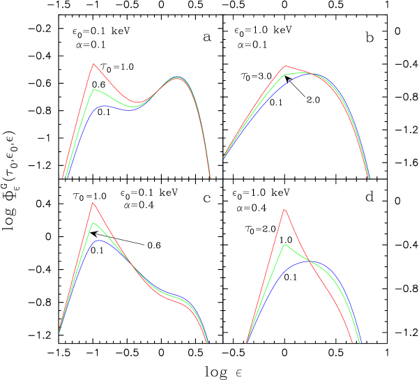
Figure 4: Column-integrated Green’s function $\Phi_{\epsilon}^{\rm G}$ ($\rm s^{-1}\,keV^{-1}$) describing the photon number spectrum escaping from an accretion column as a function of the radiation energy $\epsilon$ (keV) and the source optical depth $\tau_{0}$, evaluated using eq. (73). The curves were computed by setting $\sigma_{\|}=10^{-3}\,\sigma_{{}_{\rm T}}$, $\sigma_{\perp}=\sigma_{{}_{\rm T}}$, $\overline{\sigma}=0.1\,\sigma_{{}_{\rm T}}$, $\dot{N}_{0}=1$, $\xi=2/\sqrt{3}$, $r_{0}=10^{4}\,$cm, and $T_{e}=10^{7}\,$K. The values of $\tau_{0}$, $\epsilon_{0}$, and $\alpha$ are indicated for each plot.

In Figure 4 we use equation (73) to plot the dependence of the column-integrated Green’s function $\Phi_{\epsilon}^{\rm G}$ on the radiation energy $\epsilon$ using the same parameter values employed in Figure 3, along with several values for the source optical depth $\tau_{0}$, where the monochromatic seed photons are injected. In each case, we set $\sigma_{\|}=10^{-3}\,\sigma_{{}_{\rm T}}$, $\sigma_{\perp}=\sigma_{{}_{\rm T}}$, $\overline{\sigma}=0.1\,\sigma_{{}_{\rm T}}$, $\dot{N}_{0}=1$, $\xi=2/\sqrt{3}$, $r_{0}=10^{4}\,$cm, and $T_{e}=10^{7}\,$K. For the cases with $\epsilon_{0}=0.1\,$keV, thermal Comptonization produces a Wien hump at $\epsilon\sim 1\,$keV, which is the same behavior noted in Figure 3. When $\alpha=0.4$, the Wien hump is less prominent due to the effect of bulk Comptonization. In general, smaller values of the source optical depth $\tau_{0}$ result in more thermal Comptonization because the scattering plasma is more dense. Conversely, for large values of $\tau_{0}$, bulk Comptonization tends to produce a power-law spectral shape around the photon injection energy. In each case, numerical integration of $\Phi_{\epsilon}^{\rm G}$ with respect to the radiation energy $\epsilon$ confirms that the total number of photons escaping from the column per unit time is equal to unity, which is correct since we have set $\dot{N}_{0}=1$.

5.4 Column-Integrated Spectrum for an Arbitrary Source

The vertically-integrated photon spectrum emitted through the walls of the accretion column due to an arbitrary source $Q$ is given by (cf. eq. [71])

$$\Phi_{\epsilon}(\epsilon)\equiv\int_{0}^{\infty}\dot{N}_{\epsilon}(z,\epsilon)\,dz\ ,$$ (76)

where $\dot{N}_{\epsilon}$ is the altitude-dependent particular solution for the escaping photon spectrum computed using equation (70). By substituting for $\dot{N}_{\epsilon}$ using equation (70), interchanging the order of integration, and applying equation (71), we find that the particular solution for the column-integrated spectrum can be written as

$$\Phi_{\epsilon}(\epsilon)=\int_{0}^{\infty}\int_{0}^{\infty}{\Phi_{\epsilon}^{\rm G}(z_{0},\epsilon_{0},\epsilon)\over\dot{N}_{0}}\ \epsilon_{0}^{2}\,Q(z_{0},\epsilon_{0})\,d\epsilon_{0}\,dz_{0}\ ,$$ (77)

where $\Phi_{\epsilon}^{\rm G}$ is evaluated using equation (73), with $\tau_{0}$ computed in terms of $z_{0}$ using equation (28). Equation (77) facilitates the calculation of the total photon spectrum emitted by the entire column as a function of the photon energy $\epsilon$, for any source $Q$. In § 7 we examine the nature of the source term for the various emission processes important in X-ray pulsar accretion columns, and we derive associated results for the column-integrated escaping photon spectrum, $\Phi_{\epsilon}$. Astrophysical applications of these results and comparisons with the X-ray data for specific pulsars are presented in § 8.

6 MODEL PARAMETERS AND CONSTRAINTS

Our model includes a number of free parameters, such as the column radius, $r_{0}$, the temperature of the gas in the thermal mound, $T_{\rm th}$, the temperature of the electrons in the optically thin region above the mound, $T_{e}$, the magnetic field strength, $B$, and the accretion rate, $\dot{M}$. There are also several additional theory parameters that are related to the above mentioned physical parameters, including $\alpha$, $\delta$, $\xi$, and the scattering cross sections $\sigma_{\perp}$, $\sigma_{\|}$, and $\overline{\sigma}$. In this section we investigate the relationships between these various quantities, and we also introduce several new constraints that are used to reduce the number of free parameters. Based on these results, we show that for given values of the stellar mass $M_{*}$ and radius $R_{*}$, the only quantities that need to be varied when fitting the spectral data for a particular source are the six parameters $T_{e}$, $\dot{M}$, $r_{0}$, $B$, $\delta$, and $\xi$.

6.1 Dynamical Constraints

At large distances from the star, where radiation pressure effects become negligible, we require that the approximate velocity given by equation (29) equal the local free-fall velocity. We use this condition to calculate the altitude, $z_{\rm max}$, at the upper surface of the radiating region within the accretion column by writing

$$\left(2\,GM_{*}\over R_{*}+z_{\rm max}\right)^{1/2}=c\,\alpha\,\tau_{\rm max}\ ,$$ (78)

where the left-hand side represents the free-fall velocity from infinity to the top of the radiative zone. The corresponding optical depth, $\tau_{\rm max}$, is related to $z_{\rm max}$ via (see eq. [28])

$$\tau_{\rm max}=\left(\sigma_{\|}\over\sigma_{\perp}\right)^{1/4}\left(2\,z_{\rm max}\over\alpha\,\xi\,r_{0}\right)^{1/2}\ .$$ (79)

By using equation (79) to substitute for $\tau_{\rm max}$ in equation (78), we are able to derive a quadratic equation for $z_{\rm max}$ with solution

$$z_{\rm max}={R_{*}\over 2}\,\left[\left(1+C_{1}\right)^{1/2}-1\right]\ ,$$ (80)

where

$$C_{1}\equiv{4\,GM_{*}\,r_{0}\,\xi\over\alpha\,c^{2}R_{*}^{2}}\left(\sigma_{\perp}\over\sigma_{\|}\right)^{1/2}\ .$$ (81)

We will use this result to set the upper limit for the spatial integrations performed in § 7 when we calculate the emergent spectra resulting from the Comptonization of bremsstrahlung and cyclotron seed photons.

6.2 Scattering Cross Sections

Several electron scattering cross sections are incorporated into the model, based on the direction of propagation of the photon. The cross sections for photons propagating parallel and perpendicular to the magnetic field direction are denoted by $\sigma_{\|}$ and $\sigma_{\perp}$, respectively, and the angle-averaged cross section is $\overline{\sigma}$. Following Wang & Frank (1981), we set the perpendicular cross section equal to the Thomson value, so that (see eq. [7])

$$\sigma_{\perp}=\sigma_{{}_{\rm T}}\ .$$ (82)

For given values of the parameters $\dot{M}$, $r_{0}$, and $\xi$, we can compute the parallel cross section $\sigma_{\|}$ by using equation (26) to write

$$\sigma_{\|}=\left(\pi r_{0}\,m_{p}\,c\over\dot{M}\,\xi\right)^{2}{1\over\sigma_{\perp}}\ .$$ (83)

Once values are specified for the electron temperature $T_{e}$ and the parameters $\alpha$ and $\delta$, we can compute the angle-averaged cross section $\overline{\sigma}$ by using equation (38), which yields

$$\overline{\sigma}={\alpha\over 3}\,{m_{e}c^{2}\over kT_{e}}\,{\sigma_{\|}\over\delta}\ ,$$ (84)

where $\sigma_{\|}$ is evaluated using equation (83). We shall use equations (82), (83), and (84) to set the values of the three scattering cross sections appearing in our model. In general, we expect that $\sigma_{\|}\ll\overline{\sigma}\ll\sigma_{\perp}$ (e.g., Canuto et al. 1971), and this result will be verified when specific numerical models are developed. We will also confirm that the values obtained for $\sigma_{\|}$ are reasonably consistent with the dependence on the mean photon energy expressed by equation (6).

6.3 Thermal Mound Properties

The blackbody surface of the thermal mound represents the effective photosphere for photon creation and destruction in the accretion column, which occurs mainly via free-free emission and absorption. The altitude at the top of the mound can therefore be estimated by setting the free-free optical thickness across the column equal to unity,

$$\tau^{\rm ff}\equiv r_{0}\,\alpha_{\rm R}^{\rm ff}=1\ ,$$ (85)

where $\alpha_{\rm R}^{\rm ff}$ denotes the Rosseland mean of the free-free absorption coefficient. In principle, we should use an expression for $\alpha_{\rm R}^{\rm ff}$ that accounts for the effect of the strong magnetic field (e.g., Lauer et al. 1983). However, the modifications introduced by the presence of the field are relatively minor for photons with energies $\epsilon\ll kT_{e}$, which are the most strongly absorbed. We can therefore estimate the value of $\alpha_{\rm R}^{\rm ff}$ at the mound surface in the case of pure, fully-ionized hydrogen by using equation (5.20) from Rybicki & Lightman (1979) to write

$$\alpha_{\rm R}^{\rm ff}=6.10\times 10^{22}\ T_{\rm th}^{-7/2}\ \rho_{\rm th}^{2}$$ (86)

in cgs units, where $T_{\rm th}$ and $\rho_{\rm th}$ represent the temperature and density at the top of the mound, respectively, and we have set the Gaunt factor equal to unity.

By combining equations (85) and (86), we find that the density at the thermal mound surface is given by

$$\rho_{\rm th}=4.05\times 10^{-12}\ T_{\rm th}^{7/4}\ r_{0}^{-1/2}\ .$$ (87)

The inflow speed at the mound surface, $v_{\rm th}\equiv-v(z_{\rm th})$, is related to $\rho_{\rm th}$ via the continuity equation (19), which yields

$$v_{\rm th}=7.86\times 10^{10}\ \dot{M}\,r_{0}^{-3/2}\,T_{\rm th}^{-7/4}\ .$$ (88)

We can now compute the optical depth at the top of the thermal mound by combining equations (29), (32), and (88), which yields

$$\tau_{\rm th}=2.64\times 10^{28}\,{\dot{M}\,R_{*}\over M_{*}\,r_{0}^{3/2}\,T_{\rm th}^{7/4}\,\xi}\ .$$ (89)

The corresponding altitude, $z_{\rm th}$, is obtained by combining equations (28), (32), and (89), which yields in cgs units

$$z_{\rm th}=5.44\times 10^{15}\,{\dot{M}\,R_{*}\over M_{*}\,r_{0}\,T_{\rm th}^{7/2}\,\xi\,\sigma_{\|}}\ .$$ (90)

We will use $z_{\rm th}$ as the lower limit for the spatial integrations performed in § 7 when we calculate the emergent spectra resulting from the Comptonization of bremsstrahlung and cyclotron seed photons.

The temperature of the gas in the thermal mound, $T_{\rm th}$, is computed separately from the temperature of the electrons, $T_{e}$, in the optically thin region above the mound, although the two temperatures are expected to be comparable. We calculate $T_{\rm th}$ by setting the downward flux of kinetic energy at the mound surface equal to the upward flux of blackbody radiation, i.e.,

$$\sigma_{{}_{\rm SB}}\,T_{\rm th}^{4}={1\over 2}\,J\,v_{\rm th}^{2}\ ,$$ (91)

where

$$J\equiv\rho_{\rm th}\,v_{\rm th}={\dot{M}\over\pi r_{0}^{2}}$$ (92)

denotes the (constant) mass accretion flux and $\sigma_{{}_{\rm SB}}$ is the Stephan-Boltzmann constant. The right-hand side of equation (91) represents the flux of kinetic energy that must be thermalized and radiated by the mound before the gas can merge onto the star. By combining equations (19), (88), and (91), we find that the mound temperature is given in cgs units by

$$T_{\rm th}=2.32\times 10^{3}\,\dot{M}^{2/5}\,r_{0}^{-2/3}\ .$$ (93)

Once values for the fundamental free parameters $M_{*}$, $R_{*}$, $\dot{M}$, $r_{0}$, and $\xi$ have been selected, the mound temperature $T_{\rm th}$ is evaluated using equation (93), after which the velocity $v_{\rm th}$, optical depth $\tau_{\rm th}$, and altitude $z_{\rm th}$ at the mound surface are calculated using equations (88), (89), and (90), respectively.

6.4 Bulk vs. Thermal Comptonization

The dimensionless parameter $\delta$ defined by equation (38) plays a central role in determining the overall shape of the reprocessed radiation spectrum resulting from the bulk and thermal Comptonization of the seed photons. We demonstrate here that $\delta$ is essentially the ratio of the “$y$-parameters” for these two processes. In the one-dimensional flow configuration under consideration here, the mean energization rate for a photon with energy $\epsilon$ due to the bulk compression of the decelerating electrons is given by (e.g., Becker 1992)

$$\left\langle{d\epsilon\over dt}\right\rangle\bigg{|}_{\rm bulk}=-\,{\epsilon\over 3}\,{dv\over dz}={\alpha\,c\,n_{e}\sigma_{\|}\,\epsilon\over 3}\ ,$$ (94)

where the final result is obtained by utilizing equation (24), along with the approximate velocity profile given by equation (27). The associated $y$-parameter, describing the average fractional energy change experienced by a photon before it escapes through the column walls, is defined by

$$y_{\rm bulk}\equiv{t_{\rm esc}\over\epsilon}\,\left\langle{d\epsilon\over dt}\right\rangle\bigg{|}_{\rm bulk}={\alpha\,c\,n_{e}\sigma_{\|}\,t_{\rm esc}\over 3}\ ,$$ (95)

where $t_{\rm esc}$ is the mean escape timescale, expressed as a function of $z$ by equation (65).

Next we recall that the mean stochastic energization rate for the thermal Comptonization of photons is given by (Rybicki & Lightman 1979)

$$\left\langle{d\epsilon\over dt}\right\rangle\Bigg{|}_{\rm therm}=n_{e}\,\overline{\sigma}\,c\ \epsilon\ {4kT_{e}\over m_{e}c^{2}}\ ,$$ (96)

with associated $y$-parameter defined by

$$y_{\rm therm}\equiv{t_{\rm esc}\over\epsilon}\,\left\langle{d\epsilon\over dt}\right\rangle\bigg{|}_{\rm therm}=n_{e}\,\overline{\sigma}\,c\ t_{\rm esc}\ {4kT_{e}\over m_{e}c^{2}}\ .$$ (97)

We note that $n_{e}\propto v^{-1}\propto z^{-1/2}$ and $t_{\rm esc}\propto z^{-1/2}$ according to equations (29) and (65), respectively. Hence, $y_{\rm bulk}$ and $y_{\rm therm}$ each vary in proportion to $z^{-1}$, and therefore both quantities diverge at the base of the column. It is therefore difficult to assign global values for the two parameters that characterize the entire accretion column.

We can gain insight into the relative importance of bulk and thermal Comptonization by relating the ratio of the respective $y$-parameters to the value of $\delta$ by combining equations (38), (95), and (96), which yields

$${\delta\over 4}={y_{\rm bulk}\over y_{\rm therm}}\ .$$ (98)

According to this relation, bulk Comptonization dominates the photon energization if $\delta\gg 1$, and thermal Comptonization dominates if $\delta\ll 1$. In the intermediate regime, with $\delta\sim 1$, both processes contribute about equally to the energy transfer between the electrons and the photons. However, it is important to realize that even for large values of $\delta$, the thermal process may still have a profound effect on the overall shape of the spectrum by transferring energy from high to low frequency photons, which produces a quasi-exponential cutoff at high energies and a concomitant flattening of the spectrum at lower energies.

By combining equations (94) and (96) with equation (7.36) from Rybicki & Lightman (1979), we find that the total (mean) photon energization rate for the thermal+bulk Comptonization model considered here is given by

$$\left\langle{d\epsilon\over dt}\right\rangle\Bigg{|}_{\rm total}=n_{e}\,\overline{\sigma}\,c\,\epsilon\left({4kT_{e}\over m_{e}c^{2}}-{\epsilon\over m_{e}c^{2}}+{\alpha\,\sigma_{\|}\over 3\,\overline{\sigma}}\right)\ ,$$ (99)

where the terms on the right-hand side describe the effects of stochastic energization, electron recoil losses, and bulk Comptonization, respectively. The total energization rate vanishes at the critical energy

$$\epsilon_{\rm crit}=4kT_{e}+{\alpha\,\sigma_{\|}\over 3\,\overline{\sigma}}\ m_{e}\,c^{2}\ .$$ (100)

In the low-temperature limit, we find that bulk Comptonization balances recoil losses at the energy

$$\epsilon_{\rm bulk}={\alpha\,\sigma_{\|}\over 3\,\overline{\sigma}}\ m_{e}\,c^{2}\ ,\ \ \ \ T_{e}\to 0\ ,$$ (101)

which is the maximum photon energy achieved in the thermal+bulk model as $T_{e}\to 0$. Note that in the pure bulk Comptonization model of Becker & Wolff (2005a,b), recoil losses are not included, and therefore the power-law shape extends to infinite photon energy. This makes it necessary to restrict the index of the photon spectrum to $\alpha_{\rm X}>2$ in order to avoid an infinite photon energy density in the Becker & Wolff model. However, no such restriction exists in the thermal+bulk model considered here because recoil losses always attenuate the spectrum at high photon energies.

6.5 Photon Advection, Diffusion, and Escape

The seed photons injected into the accretion column experience a variety of physical effects as they propagate within the plasma, eventually escaping through the column walls. In this section we will show that in a radiation-dominated accretion column, the timescale for the escape of radiation through the column walls is comparable to the dynamical timescale for the accretion of the gas onto the star. In particular, we will demonstrate that the dimensionless parameter $\xi$ defined in equation (26) is proportional to the ratio of these two timescales.

We define the dynamical timescale, $t_{\rm shock}$, for the accretion of material from the sonic point down to the surface of the star by writing

$$t_{\rm shock}\equiv{z_{\rm sp}\over v(z_{\rm sp})}\ ,$$ (102)

where $z_{\rm sp}$ is the distance between the sonic point and the stellar surface given by equation (31). We can form the ratio of the dynamical timescale $t_{\rm shock}$ to the mean escape timescale $t_{\rm esc}$ for photons to diffuse through the walls of the accretion column by employing equations (18) and (102), which yields

$${t_{\rm shock}\over t_{\rm esc}}={\pi\,m_{p}\,c\,z_{\rm sp}\over\dot{M}\,\sigma_{\perp}}\ .$$ (103)

We can substitute for $\dot{M}$ and $z_{\rm sp}$ using equations (26) and (31), respectively, to obtain the alternative result

$${t_{\rm shock}\over t_{\rm esc}}={\ln(7/3)\over 2\sqrt{3}}\ \xi\sim 0.24\ \xi\ .$$ (104)

Becker (1998) found that $\xi=2/\sqrt{3}$ in a radiation-dominated pulsar accretion flow, and therefore we conclude that

$$t_{\rm shock}\sim 0.28\ t_{\rm esc}\ .$$ (105)

This result is expected, since the timescale for the photons to escape from the column must be comparable to the dynamical timescale because the radiation must be able to remove the kinetic energy from the flow. This is a general property of radiative accretion flows (see, e.g., Imamura et al. (1987).

We can gain additional insight into the processes affecting the transport of photons through the accretion column by analyzing the relative importance of the upward diffusion of photons along the column axis, compared with the downward advection of photons caused by the “trapping” of radiation in the rapidly falling gas. The parameter $\xi$ defined in equation (26) also provides a direct measurement of the influence of these two competing effects. The mean diffusion velocity for photons propagating parallel to the axis of the accretion column, $w_{||}$, can be approximated by writing

$$w_{||}={c\over\tau}\ .$$ (106)

Photon “trapping” occurs when the downward advective flux dominates over the upward diffusive flux, so that the photons are essentially confined in the lower region of the flow (Becker & Begelman 1986). In the model considered here, we find that the radiation is trapped if $|v|>w_{||}$, which can be rewritten using equations (27) and (106) as the condition $\tau>\tau_{\rm trap}$, where

$$\tau_{\rm trap}={1\over\sqrt{\alpha}}\ .$$ (107)

In the lower region of the column, where $\tau<\tau_{\rm trap}$, diffusion is able to transport radiation effectively in the vertical direction. We can calculate the associated “trapping altitude” for photons diffusing vertically in the column by combining equations (28) and (107), which yields

$$z_{\rm trap}={\pi r_{0}^{2}\,c\,m_{p}\over 2\dot{M}\sigma_{\|}}={r_{0}\,\xi\over 2}\left(\sigma_{\perp}\over\sigma_{\|}\right)^{1/2}\ ,$$ (108)

where the final result is obtained by substituting for $\dot{M}$ using equation (26). It is interesting to compare the value of $z_{\rm trap}$ with the distance from the stellar surface to the sonic point, $z_{\rm sp}$, given by equation (31). We find that the ratio of these two quantities is given by

$${z_{\rm trap}\over z_{\rm sp}}={\xi\,\sqrt{3}\over\ln(7/3)}\ \sim\ 2.0\ \xi\ .$$ (109)

Since $\xi\sim 1$ in a radiation-dominated pulsar accretion flow, equation (109) indicates that $z_{\rm sp}$ and $z_{\rm trap}$ are comparable, and therefore the photons are not able to penetrate very far into the region above the sonic point. Hence most of the photons escape through the walls of the column below the sonic point, with a mean residence time equal to the dynamical time for the gas to settle onto the stellar surface (see eq. [105]).

6.6 Radius of the Accretion Column

In our model, the radius $r_{0}$ of the accretion column (which is also the radius of the “hot spot” on the stellar surface) is treated as a free parameter. However, it is possible to constrain the value of this radius based on dynamical considerations related to the magnetically-channeled accretion of the gas onto the neutron star. For example, by taking into account the effects of both the stellar rotation and the strong magnetic field, Lamb et al. (1973) find that the radius of the hot spot satisfies the constraint (see also Harding et al. 1984)

$$r_{0}\lower 1.72218pt\hbox{$\;\buildrel<\over{\scriptstyle\sim}\;$}R_{*}\left(R_{*}\over r_{\rm A}\right)^{1/2}\ ,$$ (110)

where $R_{*}$ is the stellar radius and $r_{\rm A}$ is the Alfvén radius, given in cgs units by

$$r_{\rm A}=2.6\times 10^{8}\left(B\over 10^{12}\,{\rm G}\right)^{4/7}\left(R_{*}\over 10\,{\rm km}\right)^{10/7}\left(M_{*}\over M_{\odot}\right)^{1/7}\left(L_{\rm X}\over 10^{37}\,{\rm ergs\ s}^{-1}\right)^{-2/7}\ .$$ (111)

By combining equations (9), (110), and (111), we find that column radius $r_{0}$ is bounded by the upper limit

$$r_{0}\lower 1.72218pt\hbox{$\;\buildrel<\over{\scriptstyle\sim}\;$}6.5\times 10^{4}\left(B\over 10^{12}\,{\rm G}\right)^{-2/7}\left(R_{*}\over 10\,{\rm km}\right)^{9/14}\left(M_{*}\over M_{\odot}\right)^{1/14}\left(\dot{M}\over 10^{17}\,{\rm g\ s}^{-1}\right)^{1/7}\ ,$$ (112)

which represents an interesting constraint for our model. We will compare our results for $r_{0}$ with this upper bound when specific numerical models are developed in § 8.

6.7 Comparison of Exact and Approximate Velocity Profiles

Following Lyubarskii & Sunyaev (1982), we have adopted the approximate velocity profile given by equation (29), which faciliates the separation of the transport equation. The approximate velocity profile was compared with the exact solution (eq. [30]) in Figure 2, from which we conclude that the two functions agree fairly well in the radiative portion of the accretion column. We can further explore the validity of equation (29) by comparing the results obtained for the emergent spectra using the exact and approximate velocity profiles. This can be accomplished by contrasting the spectra computed using the thermal+bulk Comptonization model developed here (based on the approximate velocity distribution) with tho corresponding results obtained using the “pure” bulk Comptonization model discussed by Becker & Wolff (2005b), which is based on the exact velocity profile.

In Figure 5 we display the results obtained for the column-integrated Green’s function, $\Phi_{\epsilon}^{\rm G}$, calculated using either the thermal+bulk Comptonization model (eq. [73]) or the pure bulk Comptonization model (eq. [81] from Becker & Wolff 2005b). The parameters values employed are the same ones adopted in Figure 3, with $\epsilon_{0}=0.01\,$keV, $\alpha=0.4$, $\sigma_{\|}=10^{-3}\,\sigma_{{}_{\rm T}}$, $\sigma_{\perp}=\sigma_{{}_{\rm T}}$, $\overline{\sigma}=0.1\,\sigma_{{}_{\rm T}}$, $\dot{N}_{0}=1$, $\xi=2/\sqrt{3}$, $\tau_{0}=0.1$, and $r_{0}=10^{4}\,$cm. The electron temperature $T_{e}$ is set equal to $10^{7}\,$K, $10^{6.3}\,$K, $10^{5.3}\,$K, or 0, and the corresponding values for $\delta$ are 0.79, 3.95, 39.54, and $\infty$, respectively (see eq. [38]). Note that a Wien hump forms at energy $\epsilon\sim\epsilon_{\rm crit}$ (eq. [100]) for large values of $T_{e}$ due to photon energy redistribution, and as $T_{e}\to 0$ the spectrum approaches the power-law shape characteristic of bulk Comptonization. The high-energy cutoffs displayed by the spectra in Figure 5 are the result of electron recoil only; in actual X-ray pulsar spectra, the quasi-exponential cutoffs are produced by a combination of electron recoil and cyclotron absorption, as discussed in § 8.

The Becker & Wolff (2005b) spectrum is based on the exact velocity solution (eq. [30]), and therefore it provides an interesting test for the model considered here, which is based on the approximate velocity profile (eq. [29]). In the limit $T_{e}\to 0$, bulk Comptonization dominates the spectral formation process, and the column-integrated Green’s function computed using equation (73) agrees perfectly with the Becker & Wolff result up to photon energy $\epsilon=\epsilon_{\rm bulk}$, defined as the energy at which bulk Comptonization is balanced by losses due to electron recoil (see eq. [101]). Since recoil losses were not included in the Becker & Wolff (2005b) model, the resulting spectrum extends to infinite photon energy. Similar agreement between the two models in the low-temerature limit has been confirmed using several other sets of parameters. These comparisons confirm that the approximate velocity profile utilized here provides a good representation of the effect of bulk Comptonization in the pulsar accretion column.

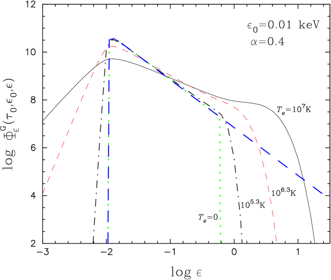
Figure 5: Column-integrated Green’s function $\Phi_{\epsilon}^{\rm G}$ ($\rm s^{-1}\,keV^{-1}$) describing the photon number spectrum escaping from an accretion column as a function of the radiation energy $\epsilon$ (keV) and the electron temperature $T_{e}$, evaluated using eq. (73). The results were computed by setting $\epsilon_{0}=0.01\,$keV, $\alpha=0.4$, $\sigma_{\|}=10^{-3}\,\sigma_{{}_{\rm T}}$, $\sigma_{\perp}=\sigma_{{}_{\rm T}}$, $\overline{\sigma}=0.1\,\sigma_{{}_{\rm T}}$, $\dot{N}_{0}=1$, $\xi=2/\sqrt{3}$, $\tau_{0}=0.1$, and $r_{0}=10^{4}\,$cm. The corresponding value of $T_{e}$ is indicated for each curve, and the heavy dashed line denotes the spectrum obtained using the exact velocity profile; see the discussion in the text.

7 PHOTON SOURCES AND ASSOCIATED SPECTRA

The high-energy radiation spectrum emerging from an X-ray pulsar accretion column is produced via the bulk and thermal Comptonization of seed photons injected into the plasma by a variety of emission mechanisms. Based on the linearity of the transport equation (15), we can compute the radiation spectrum emerging from the accretion column for any source term $Q$ by employing the integral convolutions given by equations (70) and (77) for the altitude-dependent and column-integrated spectra $\dot{N}_{\epsilon}(z,\epsilon)$ and $\Phi_{\epsilon}(\epsilon)$, respectively. The calculation of the two spectra is straightforward due to the availability of the analytical solutions for the altitude-dependent Green’s function $\dot{N}_{\epsilon}^{\rm G}$ (eq. [68]) and for the column-integrated Green’s function $\Phi_{\epsilon}^{\rm G}$ (eq. [73]). In the context of accretion-powered X-ray pulsars, the primary sources of seed photons are bremsstrahlung, cyclotron, and blackbody radiation (Arons et al. 1987). The first two mechanisms inject photons throughout the column, although the emission tends to be concentrated towards the base of the column because of the strong density dependence of these processes. Conversely, blackbody radiation is injected primarily at the surface of the thermal mound (i.e., the “photosphere”), where the gas achieves thermodynamic equilibrium. The energy dependences of the three emission mechanisms are also quite different, with the bremsstrahlung and blackbody processes producing broadband continuum radiation, and the cyclotron producing nearly monochromatic radiation.

The nature of the source term $Q$ appearing in the transport equation (15) is examined in detail below for each of the emission mechanisms of interest here. In general, $Q$ can be related to the photon emissivity, $\dot{n}_{\epsilon}$, by writing

$$\epsilon^{2}\,Q(z,\epsilon)\,d\epsilon\,dz=\pi r_{0}^{2}\,\dot{n}_{\epsilon}\,d\epsilon\,dz\ ,$$ (113)

where $\dot{n}_{\epsilon}\,d\epsilon$ expresses the number of photons created per unit time per unit volume in the energy range between $\epsilon$ and $\epsilon+d\epsilon$. We will use equation (113) to determine $Q$ by specifying the emissivity $\dot{n}_{\epsilon}$ for bremsstrahlung, cyclotron, and blackbody emission. In our approach, we treat the cyclotron and bremsstrahlung sources as separate emission mechanisms, although they can also be viewed as components of a single, generalized magneto-bremsstrahlung process, as discussed by Riffert et al. (1999).

7.1 Cyclotron Radiation

In an accretion-powered X-ray pulsar, cyclotron photons are produced mainly as a result of the collisional excitation of electrons to the $n=1$ Landau level, followed by radiative decay to the ground state ($n=0$). The electrons are excited via collisions with protons, and therefore the production of the cyclotron radiation is a two-body process. Estimates suggest that in the luminous sources, collisional deexcitation is completely negligible compared with radiative deexcitation, and therefore the production of the cyclotron radiation acts as a cooling mechanism for the gas (e.g., Nagel 1980). The subsequent Comptonization of these photons results in further cooling. The cyclotron line will be broadened by thermal effects, as well as the possible spatial variation of the magnetic field, but these effects are likely to be masked by the strong diffusion in energy space caused by thermal Comptonization. We can therefore approximate the distribution of the cyclotron seed photons using a monochromatic source term. Based on equations (7) and (11) from Arons et al. (1987), we find that in the case of pure, fully-ionized hydrogen, the rate of production of cyclotron photons per unit volume per unit energy is given in cgs units by

$$\dot{n}_{\epsilon}^{\rm cyc}=2.10\times 10^{36}\,\rho^{2}\,B_{12}^{-3/2}\,H\left(\epsilon_{c}\over kT_{e}\right)\,e^{-\epsilon_{c}/kT_{e}}\,\delta(\epsilon-\epsilon_{c})\ ,$$ (114)

where the cyclotron energy $\epsilon_{c}$ is defined by equation (1), and

$$H\left(\epsilon_{c}\over kT_{e}\right)\equiv\cases{0.41\ ,&$\epsilon_{c}/kT_{e}>7.5$ \ ,\cr 0.15\,\sqrt{\epsilon_{c}/kT_{e}}\ ,&$\epsilon_{c}/kT_{e}<7.5$ \ .\cr}$$ (115)

The cyclotron line will be broadened by thermal effects, as well as the possible spatial variation of the magnetic field, but these effects are likely to be masked by the strong diffusion in energy space caused by thermal Comptonization. We can therefore approximate the cyclotron source term, $Q^{\rm cyc}$, using the monochromatic expression

$$Q^{\rm cyc}(z,\epsilon)\equiv 1.92\times 10^{52}\,r_{0}^{2}\,\rho^{2}\,B_{12}^{-7/2}\,H\left(\epsilon_{c}\over kT_{e}\right)\,e^{-\epsilon_{c}/kT_{e}}\,\delta(\epsilon-\epsilon_{c})\ ,$$ (116)

obtained by combining equations (113) and (114).

The cyclotron source term described by equation (116) is localized in energy and distributed in space. Following Lyubarskii & Sunyaev (1982), we assume that the electrons in the optically thin plasma above the thermal mound are isothermal, and we also assume that the magnetic field $B$ has a cylindrical geometry with a constant value throughout the column. The neglect of the dipole variation of the field geometry and strength is expected to have a small effect on the emergent spectrum because most of the radiation is created, reprocessed, and emitted through the column walls within one or two scattering optical depths above the stellar surface. Compared with the cylindrical geometry employed in our model, the inclusion of the actual dipole geometry of the magnetic field will tend to increase the plasma density at the bottom of the accretion column, due to the funnel-like shape of the column walls. This is likely to further increase the concentration of the radiative processes near the bottom of the column. However, a small fraction of the photons may nonetheless diffuse to a significant altitude (perhaps several kilometers) above the star before escaping, because the scattering cross section $\sigma_{\|}$ for photons propagating parallel to the magnetic field is generally much less than Thomson (see § 6.2). This issue requires further exploration using a numerical model that includes the exact dipole dependence of the magnetic field.

For a constant value of $B$, the spatial variation of the cyclotron source term reduces to $Q^{\rm cyc}\propto\rho^{2}$, which reflects the two-body nature of the collisional excitation process. We can obtain the particular solution for the column-integrated spectrum of the escaping radiation resulting from the reprocessing of the cyclotron photons by using equation (116) to substitute for $Q$ in equation (77). The energy integration is trivial, and we find after substituting for $B_{12}$ using equation (1) and integrating over $z_{0}$ that the particular solution for the column-integrated escaping photon spectrum is given in cgs units by

$$\Phi^{\rm cyc}_{\epsilon}(\epsilon) = {3.43\times 10^{-16}\dot{M}\,H(\chi_{c})\,\xi^{2}\sqrt{\alpha^{3}w}\ \epsilon^{\kappa-2}\over\overline{\sigma}\,\epsilon_{c}^{\kappa+3/2}e^{(\epsilon_{c}+\epsilon)/(2kT_{e})}}\ \sum_{n=0}^{\infty}\ {\Gamma(\mu-\kappa+1/2)\,n!\over\Gamma(1+2\mu)\,\Gamma(n+1/2)}$$

$$\times X_{n}\,A_{n}\,M_{\kappa,\mu}[\min(\chi,\chi_{c})]\,W_{\kappa,\mu}[\max(\chi,\chi_{c})]\ ,$$ (117)

where $X_{n}$ is computed using equation (75) and we have made the definitions $\chi\equiv\epsilon/kT_{e}$ and $\chi_{c}\equiv\epsilon_{c}/kT_{e}$. The quantity $A_{n}$ represents the spatial integration

$$A_{n}\equiv\int_{\tau_{\rm th}}^{\tau_{\rm max}}e^{3\alpha\tau_{0}^{2}/2}\,g_{n}(\tau_{0})\,\tau_{0}^{-1}\,d\tau_{0}\ ,$$ (118)

where $\tau_{\rm max}$ and $\tau_{\rm th}$ denote the optical depths at the top of the accretion column and the surface of the thermal mound, respectively (see eqs. [79] and [89]). By substituting for $g_{n}$ using equation (44), we find that $A_{n}$ can be evaluated analytically, yielding

$$A_{n}=\sum_{m=0}^{n}{\Gamma(n+1/2)\,(2w)^{m}\,(3-w)^{-m}\over\Gamma(m+1/2)\,2\,m!\,(n-m)!}\left\{\Gamma\left[m,{\alpha(w-3)\tau_{\rm th}^{2}\over 4}\right]-\Gamma\left[m,{\alpha(w-3)\tau_{\rm max}^{2}\over 4}\right]\right\}\ ,$$ (119)

where $\Gamma(a,z)$ denotes the incomplete gamma function.

7.2 Blackbody Radiation

Photons are produced at the surface of the thermal mound with a blackbody distribution, and therefore the surface flux is equal to $\pi$ times the intensity (Rybicki & Lightman 1979). Following Becker & Wolff (2005b), we define the function $S(\epsilon)$ so that $\epsilon^{2}S(\epsilon)\,d\epsilon$ represents the number of photons emitted from the surface per second in the energy range between $\epsilon$ and $\epsilon+d\epsilon$. We can relate $S(\epsilon)$ to the Planck distribution by expressing the amount of energy emitted per second from the surface of the thermal mound (with area $\pi r_{0}^{2}$) in the energy range between $\epsilon$ and $\epsilon+d\epsilon$ as

$$\epsilon^{3}S(\epsilon)\,d\epsilon=\pi\,r_{0}^{2}\cdot\pi\,B_{\epsilon}(\epsilon)\,d\epsilon\ ,$$ (120)

where

$$B_{\epsilon}(\epsilon)={2\,\epsilon^{3}\over c^{2}h^{3}}\,{1\over e^{\epsilon/kT_{\rm th}}-1}$$ (121)

denotes the blackbody intensity and $T_{\rm th}$ is the temperature of the gas in the thermal mound. Note that the units for $B_{\epsilon}$ are ${\rm ergs\ s^{-1}\,ster^{-1}\,cm^{-2}\,erg^{-1}}$.

The function $S$ is related to the source term $Q$ appearing in the transport equation (15) via

$$Q^{\rm bb}(z,\epsilon)\equiv S(\epsilon)\,\delta(z-z_{\rm th})\ ,$$ (122)

which can be combined with equations (120) and (121) to conclude that

$$Q^{\rm bb}(z,\epsilon)={2\,\pi^{2}r_{0}^{2}\over c^{2}h^{3}}\,{\delta(z-z_{\rm th})\over e^{\epsilon/kT_{\rm th}}-1}\ .$$ (123)

This result for the blackbody source term is localized in physical space, but it possesses a distributed (continuum) energy dependence, which is the exact opposite of the cyclotron source given by equation (116).

We can obtain the particular solution for the column-integrated spectrum of the escaping radiation resulting from the reprocessing of the blackbody photons by using equation (123) to substitute for $Q$ in equation (77). In this case the spatial integration is trivial, and we find after some algebra that

$$\Phi^{\rm bb}_{\epsilon}(\epsilon)={2\,\pi^{2}r_{0}^{2}\over c^{2}h^{3}}\int_{0}^{\infty}{\Phi_{\epsilon}^{\rm G}(z_{\rm th},\epsilon_{0},\epsilon)\over\dot{N}_{0}}\ {\epsilon_{0}^{2}\,d\epsilon_{0}\over e^{\epsilon_{0}/kT_{\rm th}}-1}\ ,$$ (124)

where $\Phi_{\epsilon}^{\rm G}$ is computed using equation (73).

7.3 Bremsstrahlung Radiation

The bremsstrahlung emission spectrum produced by electrons streaming along a strong magnetic field is modified from the standard thermal result due to the appearance of the resonance at the cyclotron energy $\epsilon_{c}$ (Lauer et al. 1983). However, it can be shown that the angle-averaged emission spectrum obtained by integrating over the one-dimensional Maxwellian electron distribution in the accretion column agrees fairly well with the field-free thermal expression for photon energies $\epsilon<\epsilon_{c}$. We can therefore describe the bremsstrahlung photon source using the standard thermal formula in combination with a separate (resonant) cyclotron term described by equation (114). Based on equation (5.14b) from Rybicki & Lightman (1979), we find that the thermal component of the bremsstrahlung (free-free) photon production rate per unit volume per unit energy is given in cgs units by

$$\dot{n}_{\epsilon}^{\rm ff}=3.68\times 10^{36}\,\rho^{2}\,T_{e}^{-1/2}\,\epsilon^{-1}\,e^{-\epsilon/kT_{e}}\ ,$$ (125)

for a plasma composed of pure, fully-ionized hydrogen. Equation (125) can be combined with equation (113) to define the free-free source term

$$Q^{\rm ff}(z,\epsilon)\equiv 1.16\times 10^{37}\,r_{0}^{2}\,\rho^{2}\,T_{e}^{-1/2}\,\epsilon^{-3}\,e^{-\epsilon/kT_{e}}\ ,\ \ \ \ \ z_{\rm th}<z<z_{\rm max}\ ,$$ (126)

where $z_{\rm max}$ and $z_{\rm th}$ denote the altitudes at the top of the accretion column and the surface of the thermal mound, respectively (see § 6.1). Equation (126) describes the spectrum of the injected, optically-thin bremsstrahlung emission for photons with energy $\epsilon_{\rm abs}<\epsilon<\epsilon_{c}$, where $\epsilon_{\rm abs}$ represents the thermal self-absorption cutoff, below which the spectrum becomes optically thick. The calculation of $\epsilon_{\rm abs}$ is complicated by the fact that the soft photons created via bremsstrahlung emission may be upscattered due to collisions with fast electrons before they are reabsorbed. The energy amplification associated with electron scattering tends to enhance the survival probability of the photons because the absorption length is a rapidly increasing function of the photon energy. The effective value of $\epsilon_{\rm abs}$ can therefore be estimated by setting $\ell_{\rm sc}=1/\alpha^{\rm ff}_{\nu}$, where $\ell_{\rm sc}=(\sigma_{{}_{\rm T}}\,n_{e})^{-1}$ is the electron scattering mean free path and $\alpha^{\rm ff}_{\nu}$ is the free-free absorption coefficient given by equation (5.18b) from Rybicki & Lightman (1979). This yields

$${\epsilon_{\rm abs}\over kT_{e}}=6.08\times 10^{12}\,T_{e}^{-7/4}\,\rho^{1/2}\ .$$ (127)

The utilization of the Thomson cross section is justified because most of the bremsstrahlung photons are emitted roughly perpendicular to the magnetic field due to the dipole nature of the radiation pattern (e.g., Lauer et al. 1983). In our applications, the value adopted for $\epsilon_{\rm abs}$ is obtained by averaging equation (127) over the vertical structure of the column. We typically find that $0.01\lower 1.72218pt\hbox{$\;\buildrel<\over{\scriptstyle\sim}\;$}\epsilon_{\rm abs}/kT_{e}\lower 1.72218pt\hbox{$\;\buildrel<\over{\scriptstyle\sim}\;$}0.1$.

The bremsstrahlung source term given by equation (126) possesses distributed spatial and energy dependences, and therefore it is more challenging to implement than the cyclotron and blackbody sources given by equations (116) and (123), respectively. By using equation (126) to substitute for $Q$ in equation (77), we find after several steps that the particular solution for the column-integrated spectrum of the escaping radiation resulting from the reprocessing of the bremsstrahlung photons can be written in cgs units as

$$\Phi^{\rm ff}_{\epsilon}(\epsilon) = {2.80\times 10^{-12}\,\dot{M}\,\xi^{2}\sqrt{\alpha^{3}w}\ \epsilon^{\kappa-2}\,e^{-\epsilon/(2kT_{e})}\over\overline{\sigma}\,(kT_{e})^{\kappa+1/2}}$$ (128)

$$\quad\times\ \sum_{n=0}^{\infty}\ {\Gamma(\mu-\kappa+1/2)\,n!\over\Gamma(1+2\mu)\,\Gamma(n+1/2)}\ X_{n}\,A_{n}\,B_{n}\ ,$$

where $X_{n}$ and $A_{n}$ are computed using equations (75) and (119), respectively. The quantity $B_{n}$ represents the energy integral

$$B_{n}\equiv\int_{\chi_{\rm abs}}^{\infty}\chi_{0}^{-1-\kappa}\,e^{-\chi_{0}/2}\,M_{\kappa,\mu}[\min(\chi,\chi_{0})]\,W_{\kappa,\mu}[\max(\chi,\chi_{0})]\,d\chi_{0}\ ,$$ (129)

where $\chi\equiv\epsilon/kT_{e}$, $\chi_{0}\equiv\epsilon_{0}/kT_{e}$, and $\chi_{\rm abs}\equiv\epsilon_{\rm abs}/kT_{e}$. This integral can be evaluated analytically, but the result is very complex and therefore we do not state it here.

8 ASTROPHYSICAL APPLICATIONS

By combining results from the previous sections in the paper, we can now compute the spectrum emitted from an X-ray pulsar accretion column due to the bulk and thermal Comptonization of bremsstrahlung, cyclotron, and blackbody seed photons. The theoretical prediction for the phase-averaged photon count rate spectrum measured at Earth is computed using

$$F_{\epsilon}(\epsilon)\equiv{\Phi_{\epsilon}^{\rm tot}(\epsilon)\over 4\pi D^{2}}\ ,$$ (130)

where

$$\Phi_{\epsilon}^{\rm tot}(\epsilon)\equiv\left[\Phi^{\rm cyc}_{\epsilon}(\epsilon)+\Phi^{\rm bb}_{\epsilon}(\epsilon)+\Phi^{\rm ff}_{\epsilon}(\epsilon)\right]A_{c}(\epsilon)$$ (131)

denotes the total spectrum of the Comptonized radiation escaping from the column, $D$ is the distance to the source, and the function $A_{c}$ represents a Gaussian cyclotron absorption feature given by the form (e.g., Heindl & Chakrabarty 1999; Orlandini et al. 1998; Soong et al. 1990)

$$A_{c}(\epsilon)\equiv 1-{d_{c}\over\sigma_{c}\sqrt{2\pi}}\,e^{-(\epsilon-\epsilon_{c})^{2}/(2\sigma^{2}_{c})}\ .$$ (132)

The quantities on the right-hand side in equation (131) express the contributions to the escaping spectrum due to the reprocessing of cyclotron radiation ($\Phi^{\rm cyc}_{\epsilon}$; eq. [117]), blackbody radiation ($\Phi^{\rm bb}_{\epsilon}$; eq. [124]), and bremsstrahlung emission ($\Phi^{\rm ff}_{\epsilon}$; eq. [128]), respectively. In this section we will use equation (130) to compute observed spectra based on parameters corresponding to three specific X-ray pulsars. The theoretical spectra will be compared with the observational data for each source in order to gain insight into the effects of bulk and thermal Comptonization in the accretion shock on the formation of the X-ray continuum. The spectral results presented here are example calculations, rather than detailed quantitative fits, which will be reported in subsequent papers.

The sources treated here are Her X-1, LMC X-4, and Cen X-3, which represent several of the brightest known X-ray pulsars. In each case the values adopted for the stellar mass and radius are $M_{*}=1.4\,M_{\odot}$ and $R_{*}=10\,$km, respectively. The accretion dynamics in these high-luminosity sources is expected to be dominated by radiation pressure, and therefore we expect that $\xi\approx 2/\sqrt{3}$ (see Becker 1998). The scattering cross section for photons propagating perpendicular to the magnetic field in our calculations is given by $\sigma_{\perp}=\sigma_{{}_{\rm T}}$ (see eq. [82]), the accretion rate $\dot{M}$ is constrained by the observed X-ray luminosity, and the source distance $D$ is determined using published estimates. The remaining fundamental input parameters that must be set in order to calculate the theoretical spectrum are $\delta$, $B$, $r_{0}$, and $T_{e}$, which are listed in Table 1 for each of the models considered here. Once these quantities are specified, the additional parameters $\alpha$, $\tau_{\rm max}$, $\sigma_{\|}$, $\overline{\sigma}$, $\tau_{\rm th}$, $T_{\rm th}$, $\tau_{\rm trap}$, and $\epsilon_{\rm abs}$ can be computed using equations (33), (79), (83), (84), (89), (93), (107), and (127), respectively, with the results reported in Table 2. Note that in each case, we find that $\tau_{\rm max}\lower 1.72218pt\hbox{$\;\buildrel<\over{\scriptstyle\sim}\;$}\tau_{\rm trap}$, which indicates that the observed emission is produced in the “trapped” region of the accretion column, as expected (see § 6.5). Table 2 also includes results for the inflow speed at the thermal mound surface, $v_{\rm th}$ (eq. [88]), and the accretion mass flux, $J$ (eq. [92]). In general, we find in our applications that $v_{\rm th}\sim 0.03\,c$, which represents an enormous deceleration from the free-fall velocity $v_{\rm ff}\sim 0.6\,c$ at the top of the column. Since there is not much variation in the value of $v_{\rm th}$, we expect that the mound temperature $T_{\rm th}$ will increase with increasing $J$ (see eq. [91]).

Once all of the parameters are specified, the corresponding count-rate spectrum is evaluated using equation (130). The spectral results presented here were computed using the first five terms in the expansions (eqs. [117], [124], and [128]), which generally provide at least three decimal digits of accuracy. As a check on the numerical results for the spectral components, we confirm that the number of photons escaping from the column per unit time is exactly equal to the number injected, as required in the steady-state scenario considered here. In addition to the Comptonized spectrum evaluated using equation (130), the results for the total spectra displayed in Figures 6, 7, and 8 also include an Fe K$\alpha$ emission line modeled using the Gaussian function

$$F^{\rm K}_{\epsilon}(\epsilon)\equiv{d_{\rm K}\over\sigma_{\rm K}\sqrt{2\pi}}\,e^{-(\epsilon-\epsilon_{\rm K})^{2}/(2\sigma^{2}_{\rm K})}\ ,$$ (133)

where $d_{\rm K}$ is the associated total photon flux measured at Earth. Note that in the approach taken here, this spectral feature is treated in an ad hoc manner by simply adding it to the final spectrum rather than by subjecting the iron line photons to subsequent Comptonization. Unfortunately, a more sophisticated approach is beyond the scope of the present paper due to the complexity of the spectral formation process for the iron emission line photons. The associated auxiliary parameters $\epsilon_{\rm K}$, $d_{\rm K}$, and $\sigma_{\rm K}$ are listed in Table 3, along with $\epsilon_{c}$, $d_{c}$, and $\sigma_{c}$ (see eq. [132]).

8.1 Her X-1

In Figure 6 we display the theoretical count-rate spectrum computed using equation (130) along with the deconvolved (incident), phase-averaged BeppoSAX data reported by Dal Fiume et al. (1998) for Her X-1, which has the instrumental response removed. The values used for the fundamental theory parameters correspond to model 1, with $\xi=1.45$, $\sigma_{\perp}=\sigma_{{}_{\rm T}}$, $\delta=1.80$, $B=3.80\times 10^{12}\,$G, $r_{0}=44\,$m, $T_{e}=6.25\times 10^{7}\,$K, $\dot{M}=1.11\times 10^{17}\,\rm g\,s^{-1}$, and $D=5\,$kpc, as indicated in Table 1. The associated values for the computed parameters $\alpha$, $\tau_{\rm max}$, $\sigma_{\|}$, $\overline{\sigma}$, $\tau_{\rm th}$, and $T_{\rm th}$ are reported in Table 2, and the additional auxiliary parameters are listed in Table 3. Results are presented for the total spectrum, as well as for the individual contributions to the observed flux due to the Comptonization of cyclotron, blackbody, and bremsstrahlung seed photons. The lack of a strong Wien peak in the spectrum, along with the moderate value of $\delta$, indicate that thermal Comptonization is unsaturated in this source. It is interesting to note that the value we obtain for $r_{0}$ is about an order of magnitude below the upper limit for the column radius computed using equation (112), which yields $r_{0}\lower 1.72218pt\hbox{$\;\buildrel<\over{\scriptstyle\sim}\;$}462\,$m.

Although the results presented here are not fits to the data, it is interesting to note that the general shape of the pulsar spectrum predicted by the theory agrees very well with the observations for Her X-1, including both the quasi-exponential cutoff at high energies and the power law shape at lower energies. In the case of Her X-1, we find that reprocessed (Comptonized) blackbody emission from the thermal mound makes a relatively small contribution to the spectrum due to the small radius of the accretion column. We also find that reprocessed cyclotron emission is swamped by reprocessed bremsstrahlung due to the high temperature of the infalling plasma. Hence we conclude that the X-ray spectrum emitted by Her X-1 is completely dominated by Comptonized bremsstrahlung emission.

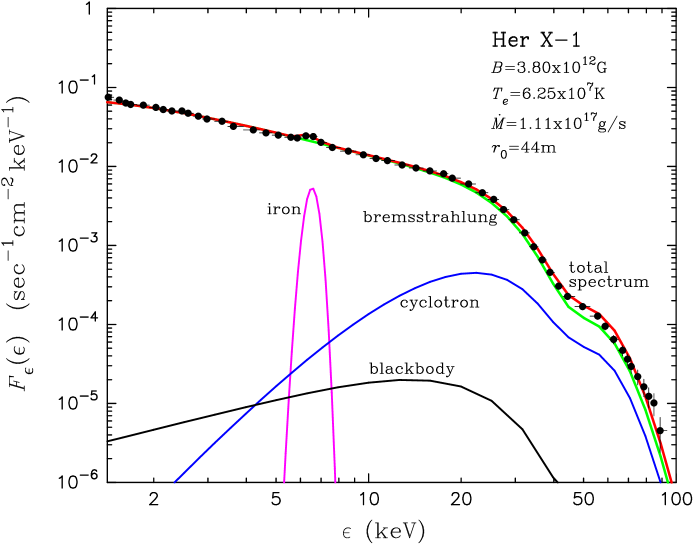
Figure 6: Theoretical column-integrated count rate spectrum $F_{\epsilon}(\epsilon)$ evaluated using eq. (130) based on the model 1 parameters listed in Table 1, compared with the deconvolved (incident) X-ray spectrum for Her X-1 reported by Dal Fiume et al. (1998; circles and crosses). The plots include the total spectrum as well as the individual components due to Comptonized bremsstrahlung radiation, Comptonized cyclotron emission, Comptonized blackbody radiation, and the iron emission line feature, as indicated. Note that the total spectrum is strongly dominated by the bremsstrahlung component.

8.2 LMC X-4

In Figure 7 we compare the theoretical count-rate spectrum computed using equation (130) with the deconvolved, phase-averaged BeppoSAX data reported by La Barbera et al. (2001) for LMC X-4. The values used for the fundamental theory parameters correspond to model 2, with $\xi=1.15$, $\sigma_{\perp}=\sigma_{{}_{\rm T}}$, $\delta=1.30$, $B=3.28\times 10^{12}\,$G, $r_{0}=680\,$m, $T_{e}=5.90\times 10^{7}\,$K, $\dot{M}=2.00\times 10^{18}\,\rm g\,s^{-1}$, and $D=55\,$kpc (see Table 1). The associated values for the computed and auxiliary parameters are listed in Tables 2 and 3, respectively. Note that the results for the accretion rate $\dot{M}$ and the column radius $r_{0}$ are much larger than those for Her X-1, although the electron temperatures are nearly the same. In this case, reprocessed cyclotron emission makes a slightly stronger contribution to the high-energy spectrum than in model 1, although the X-ray spectrum is clearly dominated by Comptonized bremsstrahlung emission. In model 2, the effect of thermal Comptonization (relative to bulk) is somewhat stronger than in model 1, as indicated by the smaller value of $\delta$ (see eq. [97]). This effect tends to flatten the LMC X-4 spectrum in the 2-22 keV energy range as compared with the Her X-1 spectrum, although the thermal Comptonization is clearly unsaturated, as demonstrated by the absence of a Wien peak in the spectrum. We also note that the reprocessed blackbody emission makes a much smaller contribution to the observed spectrum in model 2 than in model 1 because the thermal mound temperature $T_{\rm th}$ has dropped substantially, due to the marked decrease in the mass flux, $J$, as indicated in Table 2. In contrast to the Her X-1 case, for LMC X-4 we find that the value obtained for $r_{0}$ is comparable to the upper limit for the column radius computed using equation (112), which gives $r_{0}\lower 1.72218pt\hbox{$\;\buildrel<\over{\scriptstyle\sim}\;$}727\,$m. This suggests a possible connection between the column radius and the luminosity in accretion-powered X-ray pulsars that can be further explored using parameter studies based on a large number of sources.

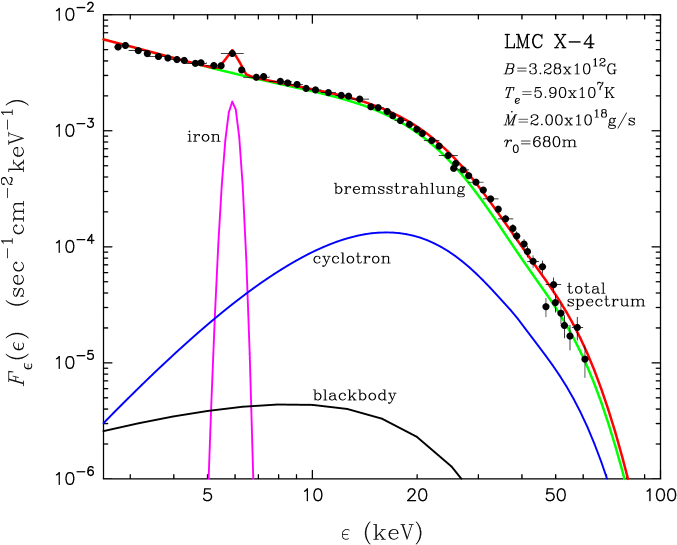
Figure 7: Same as Fig. 6, except the data correspond to LMC X-4 and the theoretical spectra were computed based on the model 2 parameters reported in Table 1. The data were reported by La Barbera et al. (2001; circles and crosses).

8.3 Cen X-3

In Figure 8 we plot the deconvolved, phase-averaged BeppoSAX data reported by Burderi et al. (2000) for Cen X-3 along with the theoretical count-rate spectrum computed using equation (130). The values adopted here for the fundamental theory parameters correspond to model 3, with $\xi=1.25$, $\sigma_{\perp}=\sigma_{{}_{\rm T}}$, $\delta=3.71$, $B=2.63\times 10^{12}\,$G, $r_{0}=730\,$m, $T_{e}=3.40\times 10^{7}\,$K, $\dot{M}=1.51\times 10^{18}\,\rm g\,s^{-1}$, and $D=8\,$kpc (see Table 1), and the additional parameters are listed in Tables 2 and 3. In this case only, interstellar absorption has been included based on a hydrogen column density of $N_{\rm H}=2.0\times 10^{22}\,{\rm cm}^{-2}$ in order to reproduce the observed low-energy turnover (cf. Burderi et al. 2000). We note that the values obtained for the accretion rate $\dot{M}$ and the column radius $r_{0}$ are once again much larger than those for Her X-1. It is apparent that the contributions due to Comptonized cyclotron and blackbody emission are completely negligible, and the observed spectrum is dominated by Comptonized bremsstrahlung photons.

The effect of bulk Comptonization is more pronounced in this case than in the spectra of Her X-1, as indicated by the larger value obtained for $\delta$. We also note that the values obtained for the accretion flux $J$ and the thermal mound temperature $T_{\rm th}$ in model 3 are lower than those associated with models 1 and 2. However, despite the decrease in the mound temperature, the Comptonized blackbody emission has increased in strength to become roughly comparable to the reprocessed cyclotron emission, which reflects the decrease in the magnetic field strength $B$. As in the case of LMC X-4, we find that the value for $r_{0}$ associated with Cen X-3 is comparable to the upper limit for the column radius computed using equation (112), which yields $r_{0}\lower 1.72218pt\hbox{$\;\buildrel<\over{\scriptstyle\sim}\;$}744\,$m. This supports the possibility of a connection between the column radius and the X-ray luminosity, as suggested in § 8.2.

9 CONCLUSIONS

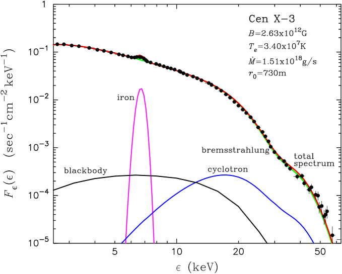
Figure 8: Same as Fig. 6, except the data correspond to Cen X-3 and the theoretical spectra were computed based on the model 3 parameters reported in Table 1. The data were reported by Burderi et al. (2000; circles and crosses). This case also includes interstellar absorption with hydrogen column density $N_{\rm H}=2.0\times 10^{22}\,{\rm cm}^{-2}$.

The new theoretical model developed here represents the first complete calculation of the X-ray spectrum associated with the physical accretion scenario first suggested by Davidson (1973), including bulk and thermal Comptonization. For given values of the stellar mass $M_{*}$ and the stellar radius $R_{*}$, our model has six fundamental free parameters, namely the accretion rate $\dot{M}$, column radius $r_{0}$, the electron temperature $T_{e}$, the magnetic field strength $B$, the photon diffusion parameter $\xi$ (eq. [26]), and the Comptonization parameter $\delta$ (eq. [38]). The accretion rate is constrained by the observed luminosity, which effectively removes this parameter from the set. A unique solution for the remaining free parameters can be found by comparing the model spectrum with the observations for a particular source. The analytical nature of the new model makes it amenable to incorporation into standard analysis packages such as XSPEC.

We have shown that the combination of bulk and thermal Comptonization naturally leads to the development of emergent spectra in accretion-powered X-ray pulsars that are in good agreement with the observational data for three bright sources. The main result of the derivation is the analytical solution for the column-integrated Green’s function describing the escaping radiation spectrum, given by equation (73). Based on this closed-form solution, we have developed expressions for the emergent spectra resulting from the reprocessing of seed photons injected as a result of cyclotron, blackbody, and bremsstrahlung emission, given by equations (117), (124), and (128), respectively (we note that additional seed photons may also be supplied via external illumination of the column, which is not considered here). In each case, we confirm that the number of photons escaping from the column per unit time is exactly equal to the number injected, as expected in the steady-state scenario considered here. Our main results, summarized in Figures 6, 7, and 8, indicate that the spectra observed from the bright sources Her X-1, LMC X-4, and Cen X-3 are dominated by Comptonized bremsstrahlung.

The treatment of the full energy and angle dependence of the scattering cross sections for the two polarization modes computed using equations (2) and (4) is not possible using an analytical approach. As an alternative, in this paper we have adopted a two-dimensional approximation by modeling the scattering of photons propagating either parallel or perpendicular to the magnetic field using the energy- and mode-averaged expressions given by equations (6) and (7), respectively. The results we have obtained for the directional components of the cross section listed in Table 2 are not unreasonable, given the uncertainties in the detailed physical properties of the accretion column. In particular, we find that the cross section for photons propagating parallel to the field direction, $\sigma_{\|}$, is substantially reduced relative to the Thomson value. This result is consistent with equation (6), since $\epsilon\ll\epsilon_{c}$ for most of the photons in typical X-ray pulsar spectra. Furthermore, the cross section values reported in Table 2 confirm that $\sigma_{\|}\ll\overline{\sigma}\ll\sigma_{\perp}$, as expected (see § 6.2 and Canuto et al. 1971). Compared to the behavior obtained in our model, we expect that utilization of the exact cross sections given by equations (2) and (4) would tend to increase the efficiency of thermal Comptonization, relative to the bulk process, for photons with energy $\epsilon$ close to the cyclotron energy $\epsilon_{c}$. This effect is therefore expected to cause some modification of the parameter values required to fit the observed X-ray pulsar spectra. Since the radiative transfer problem including the exact cross sections is not tractable analytically, further study of this issue awaits the development of a complete numerical model, which we intend to pursue in future work.

The validity of the approximate velocity profile employed here (eq. [29]) was established in Figure 5 by demonstrating excellent agreement between the bulk Comptonization spectrum computed using our new model in the limit $T_{e}\to 0$ and the corresponding spectrum obtained using the pure bulk Comptonization model of Becker & Wolff (2005b), which is based on the exact velocity profile (eq. [30]). The values obtained for the accretion column radius $r_{0}$ (reported in Table 1) comply with the corresponding upper limits computed using equation (112), which was derived based on the detailed dynamics of neutron star accretion flows (Lamb et al. 1973; Harding et al. 1984). We find that $r_{0}$ is essentially equal to the upper limit for the two brightest sources considered here (Cen X-3 and LMC X-4), while it is about an order of magnitude smaller than this limit for Her X-1. Since the luminosity of Her X-1 is roughly an order of magnitude lower then the other two sources, this suggests a possible connection between the luminosity and the column size that should be further investigated by developing numerical models that simultaneously treat the dynamics and the spectral formation in X-ray pulsars.

The transfer of energy from the gas to the photons is generally dominated by bulk Comptonization in accretion-powered X-ray pulsars. However, our results confirm that unsaturated thermal Comptonization nonetheless plays a significant role in the spectral formation process. Specifically, we find that the thermal process effectively transfers energy from high to low frequency radiation, which contributes to the observed quasi-exponential cutoffs at high energies and at the same time causes flattening of the spectrum at lower energies. While it has been known for some time that pulsars generally have spectra that are well fitted using a combination of a power-law plus a quasi-exponential cutoff, until now this form has been adopted in a purely ad hoc manner. The new model described here finally provides a firm theoretical foundation for this empirical result, based on model parameters that are directly tied to the physical properties of the source. It therefore represents a significant step in the development of a comprehensive theory for the spectral formation process in accretion-powered X-ray pulsars.

The predictions of our analytical model can be tested both observationally and also by developing numerical models that allow the relaxation of several of the key assumptions made here. For example, within the context of a numerical model one can include the exact spatial variation of the shape and strength of the dipole magnetic field, as well as the full energy and angle dependence of the electron scattering cross section. Although these effects are beyond the scope of the present paper, we nonetheless believe that our main conclusions regarding the spectral shape will be verified by more detailed models.

The authors would like to thank Ken Wolfram, Paul Ray, Lev Titarchuk, and Kent Wood for a number of stimulating conversations. The authors are also grateful to the anonymous referee who provided a number of insightful comments that led to significant improvements in the manuscript. PAB would also like to acknowledge generous support provided by the Office of Naval Research.

Table 1: Input Model Parameters

Model	Object	$\xi$	$\delta$	$B$ (G)	$\dot{M}$ (g s-1)	$T_{e}$ (K)	$r_{0}$ (m)	$D$ (kpc)
1	Her X-1	1.45	1.80	$3.80\times 10^{12}$	$1.11\times 10^{17}$	$6.25\times 10^{7}$	44.0	5.0
2	LMC X-4	1.15	1.30	$3.28\times 10^{12}$	$2.00\times 10^{18}$	$5.90\times 10^{7}$	680.0	55.0
3	Cen X-3	1.25	3.71	$2.63\times 10^{12}$	$1.51\times 10^{18}$	$3.40\times 10^{7}$	730.0	8.0

Table 2: Computed Model Parameters

Model	$\alpha$	$\sigma_{\|}/\sigma_{{}_{\rm T}}$	$\overline{\sigma}/\sigma_{{}_{\rm T}}$	$J$ (g s-1 cm-2)	$T_{\rm th}$ (K)	$v_{\rm th}/c$	$\epsilon_{\rm abs}/kT_{e}$	$\tau_{\rm th}$	$\tau_{\rm max}$	$\tau_{\rm trap}$
1	0.401	$4.15\times 10^{-5}$	$2.93\times 10^{-4}$	$1.83\times 10^{9}$	$5.68\times 10^{7}$	0.027	0.098	0.067	1.37	1.58
2	0.319	$4.85\times 10^{-5}$	$3.98\times 10^{-4}$	$1.38\times 10^{8}$	$2.91\times 10^{7}$	0.026	0.034	0.080	1.12	1.77
3	0.346	$8.30\times 10^{-5}$	$4.51\times 10^{-4}$	$9.02\times 10^{7}$	$2.48\times 10^{7}$	0.023	0.072	0.066	1.07	1.70

Table 3: Auxiliary Parameters

Model	$\epsilon_{c}$ (keV)	$\sigma_{c}$ (keV)	$d_{c}$ (keV)	$\epsilon_{\rm K}$ (keV)	$\sigma_{\rm K}$ (keV)	$d_{\rm K}$ (s-1 cm-2)
1	44.0	13.0	25.20	6.55	0.30	$4.00\times 10^{-3}$
2	38.0	21.2	38.29	5.90	0.22	$1.00\times 10^{-3}$
3	30.5	11.0	21.50	6.70	0.27	$1.20\times 10^{-2}$

References

- (1) Abramowitz, M., & Stegun, I. A. 1970, Handbook of Mathematical Functions (NY, Dover)
- (2) Arons, J., Klein, R. I., & Lea, S. 1987, ApJ, 312, 666
- (3) Basko, M. M., & Sunyaev, R. A. 1975, A&A, 42, 311
- (4) Basko, M. M., & Sunyaev, R. A. 1976, MNRAS, 175, 395
- (5) Becker, P. A., 1992, ApJ, 397, 88
- (6) Becker, P. A., 1998, ApJ, 498, 790
- (7) Becker, P. A., 2003, MNRAS, 343, 215
- (8) Becker, P. A., & Begelman, M. C. 1986, ApJ, 310, 534
- (9) Becker, P. A., & Wolff, M. T. 2005a, ApJ, 621, L45
- (10) Becker, P. A., & Wolff, M. T. 2005b, ApJ, 630, 465
- (11) Blandford, R. D., & Payne, D. G. 1981a, MNRAS, 194, 1033
- (12) Blandford, R. D., & Payne, D. G. 1981b, MNRAS, 194, 1041
- (13) Burderi, L., et al. 2000, ApJ, 530, 429
- (14) Canuto, V., Lodenquai, J., & Ruderman, M. 1971, Phys. Rev. D, 3, 2303
- (15) Chanan, G. A., Novick, R., & Silver, E. H. 1979, ApJ, 228, L71
- (16) Coburn, W., et al. 2002, ApJ, 580, 394
- (17) Colpi, M. 1988, ApJ, 326, 223
- (18) Dal Fiume, D., et al., 1998, A&A, 329, L41
- (19) Davidson, K. 1973, Nature Phys. Sci., 246, 1
- (20) di Salvo, T., Burderi, L., Robba, N. R., & Guainazzi, M. 1998, ApJ, 509, 897
- (21) Giacconi, R., et al. 1971, ApJ, 167, L67
- (22) Gradshteyn, I. S., & Ryzhik, I. M. 1980, Table of Integrals, Series, and Products (London, Academic Press)
- (23) Harding, A. K. 1994, AIP Conference Proceedings 308, ed. S. S. Holt & C. S. Day (New York: AIP), p. 429
- (24) Harding, A. K. 2003, in Pulsars, AXPs and SGRs observed with BeppoSAX and Other Observatories, ed. G. Cusumano, E. Massaro, & T. Mineo (Rome: Aracne Editrice), p. 127
- (25) Harding, A. K., et al. 1984, ApJ, 278, 369
- (26) Heindl, W. A., & Chakrabarty, D. 1999, in Highlights in X-Ray Astronomy, ed. B. Aschenbach & M. J. Freyberg, MPE Report 272 (Garching: Max-Planck-Institut f r extraterrestrische Physik), p. 25
- (27) Imamura, J. N., et al. 1987, ApJ, 313, 298
- (28) Klein, J., et al. 1996, ApJ, 457, L85
- (29) Kompaneets, A. S. 1957, Sov. Phys.–JETP, 4, 730
- (30) La Barbera, A., et al. 2001, ApJ, 553, 375
- (31) Lamb, F. K., Pethick, C. J., & Pines, D. 1973, ApJ, 184, 271
- (32) Lauer, J. et al. 1983, J. Phys. B, 16, 3673
- (33) Laurent, P., & Titarchuk, L. 1999, ApJ, 511, 289
- (34) Lyubarskii, Yu. E., & Sunyaev, R. A. 1982, Soviet Astr. Lett., 8, 330
- (35) Mészáros, P., & Nagel, W. 1985a, ApJ, 298, 147
- (36) Mészáros, P., & Nagel, W. 1985b, ApJ, 299, 138
- (37) Nagel, W. 1980, ApJ, 236, 904
- (38) Nagel, W. 1981, ApJ, 251, 288
- (39) Payne, D. G., & Blandford, R. D. 1981, MNRAS, 196, 781
- (40) Orlandini, M., et al. 1998, A&A, 332, 121
- (41) Pottschmidt, K., et al. 2005, ApJ, 634, L97
- (42) Poutanen, J., & Gierliński, M. 2003, MNRAS, 343, 1301
- (43) Riffert, H., Klingler, M., & Ruder, H. 1999, Phys. Rev. Lett., 82, 3432
- (44) Rybicki, G. B., & Lightman, A. P. 1979, Radiative Processes in Astrophysics (NY, Wiley)
- (45) Schneider, P., & Kirk, J. G. 1987, ApJ, 323, L87
- (46) Soong, Y., et al. 1990, ApJ, 348, 641
- (47) Sunyaev, R. A., & Titarchuk, L. G., 1980, A&A, 86, 121
- (48) Tananbaum, H., et al. 1972, ApJ, 174, L143
- (49) Titarchuk, L., Mastichiadis, A., & Kylafis, N. D. 1996, A&AS, 120, 171
- (50) Titarchuk, L., & Zannias, T. 1998, ApJ, 493, 863
- (51) Turolla, R., Zane, S., & Titarchuk, L. 2002, ApJ, 576, 349
- (52) Ventura, J. 1979, Phys. Rev. D, 19, 1684
- (53) Wang, Y.-M., & Frank, J. 1981, A&A, 93, 255
- (54) White, N. E., Nagase, F., & Parmar, A. N. 1995, in X-Ray Binaries, ed. W. H. G. Lewin, J. Van Paradijs, & E. P. J. Van den Heuvel (New York: Cambridge), 1
- (55) White, N. E., Swank, J. H., & Holt, S. S. 1983, ApJ, 270, 711
- (56) Yahel, R. Z. 1980, ApJ, 236, 911