Heating and Non-thermal Particle Acceleration in Relativistic, Transverse Magnetosonic Shock Waves in Proton-Electron-Positron Plasmas

Abstract

We report the results of 1D particle-in-cell simulations of ultrarelativistic shock waves in proton-electron-positron plasmas. We consider magnetized shock waves, in which the upstream medium carries a large scale magnetic field, directed transverse to the flow. Relativistic cyclotron instability of each species as the incoming particles encounter the increasing magnetic field within the shock front provides the basic plasma heating mechanism. The most significant new results come from simulations with mass ratio $m_{p}/m_{\pm}=100$. We show that if the protons provide a sufficiently large fraction of the upstream flow energy density (including particle kinetic energy and Poynting flux), a substantial fraction of the shock heating goes into the formation of suprathermal power-law spectra of $e^{-}-e^{+}$. Cyclotron absorption by the pairs of the high harmonic ion cyclotron waves, emitted by the protons, provides the non-thermal acceleration mechanism. As the proton fraction increases, the non-thermal efficiency increases and the $e^{-}-e^{+}$ power-law spectra harden.

When the proton fraction is small (pair plasma almost charge symmetric), the $e^{-}$ and $e^{+}$ have approximately equal amounts of non-thermal heating. At the lower range of our simulations with mass ratio 100, when the ions contribute 56% of the upstream flow energy flux, the pairs’ non-thermal acceleration efficiency by energy is about 1%, increasing to 5% as the ions’ fraction of upstream flow energy increases to 72%. When the fraction of upstream flow energy in the ions rises to 84%, the efficiency of non-thermal acceleration of the pairs reaches 30%, with the $e^{+}$ receiving most of the non-thermal power.

We suggest that the varying power law spectra observed in synchrotron sources that may be powered by magnetized winds and jets might reflect the correlation of the proton to pair content enforced by the underlying electrodynamics of these sources’ outflows, and that the observed correlation between the X-ray spectra of rotation powered pulsars with the X-ray spectra of their nebulae might reflect the same correlation.

1 Introduction

Collisionless shock waves in relativistic astrophysical flows have been implicated as the energizing mechanism for emission in a variety of non-thermal sources - termination shocks of pulsar winds (Slane (2005); Kaspi et al. (2004)), hot-spot shocks terminating jets from radio galaxies (Heavens & Meisenheimer (1987); Wilson, Young & Shopbell (2000); Balucińnska-Church et al. (2005)) and internal shocks in AGN and microquasar jets (Marscher & Gear (1985); Türler et al. (2000, 2004)), internal and external shocks in GRBs (Piran (2004)) and outflows from other high energy transients (e.g., Gaensler et al. (2005)). While shock jump conditions applied to models of magnetohydrodynamic flow set the constraints on what fraction of flow energy goes into heat of all sorts, the partition of that energy between ions and electrons (and positrons, when these are present), and the distributions of particle momenta (thermal or non-thermal), are kinetic questions not addressed by the macroscopic conservation laws. The kinetic questions are those of collisionless plasma physics - two body encounters cannot generate the entropy implied by the jump conditions on the observed scales of transition from non-radiative flow (upstream, in the shock excitation model) to the observed regions of synchrotron emission (downstream, in the shock model), nor can collisional processes lead to non-thermal particle spectra.

A fundamental approach in which the flow and kinetic structure of relativistic shocks are resolved on all scales offers the opportunity to evaluate the nature of the electromagnetic turbulence generated, as a function of the upstream parameters of the flow, simultaneously with a determination of the heated (possibly non-thermally accelerated) particle spectra both up and downstream. For this purpose, fully kinetic particle-in-cell (PIC) simulations (Birdsall & Langdon (1991); Dawson (1995)) provide a powerful investigatory tool, since these model the plasma from first principles, with the only approximations being those that go into the method - primarily the “cloud-in-cell” algorithm, which in effect softens the interactions to the grid scale.

PIC simulations of relativistic transverse magnetosonic shocks in a symmetric pair plasma were first reported by Langdon et al. (1988) and by Gallant et al. (1992), using spatially 1D models. Magnetized shocks are characterized by coherent gyration (Alsop & Arons (1988)) and cyclotron instability (Hoshino & Arons (1991)) of the plasma species as they encounter the shock front - magnetic reflection mediates the density and velocity transition, while the instabilty of the induced gyration mediates the entropy generation. Simulations of the Weibel instability when $B_{0}=0$ with applications to unmagnetized relativistic shocks have been reported recently by a number of authors (Silva et al. (2003); Frederiksen et al. (2004); Hededahl et al. (2004); Jaroschek (2005); Hededahl & Nishikawa (2005)). Spitkovsky and Arons (in preparation) have found comparable results, and show how the shock structures in pair plasmas depend on the magnetic field strength and orientation with respect to the flow. All these results indicate that non-thermal particle acceleration is either weak or absent in shocks in pair plasmas.

Hoshino et al. (1992) found that when the upstream flow includes heavy ions which carry a significant fraction of the upstream flow energy, non-thermal acceleration does occur, as a consequence of the absorption of ion waves emitted at harmonics of the ion cyclotron frequency reabsorbed by the pairs, even though the shock structure is one dimensional and no cross field diffusion occurred. The interaction is resonant, in contrast to the non-resonant scattering underlying Diffusive Shock Acceleration (DSA). Computational limitations required the use of a low rest mass ratio, $m_{i}/m_{\pm}=10,20$.

Those inhomogeneous shock calculations showed no electron acceleration. While most of the characteristics of the instability scale with just the energy density ratio between the protons and the pairs, the efficacy of the waves as accelerators of electrons and positrons also depends on the polarization properties of the proton cyclotron waves. The lack of electron acceleration at low mass ratio stems from the polarization of the waves excited. In a quasi-neutral pair plasma the waves are linearly polarized. If the heavy ions are a small fraction by number, the waves excited by the ion maser remain almost linearly polarized. Since linearly polarized waves are an equal mixture of left and right circularly polarized modes, equal electron and positron acceleration might have been expected. However, the simulations also revealed that the mechanism is a significant accelerator only if the energy density in the ions $U_{1i}=m_{i}N_{i1}(\gamma_{1}-1)c^{2}$, where $N_{i1}$ is the upstream ion density and $\gamma_{1}$ is the upstream flow Lorentz factor, is comparable to the upstream energy density in the pairs, $U_{1\pm}=m_{\pm}(\gamma_{1}-1)c^{2}(N_{1+}+N_{1-})$. Then $N_{1i}/(N_{1+}+N_{1-})=(m_{\pm}/m_{i})(U_{1i}/U_{1\pm})\sim m_{\pm}/m_{i}$. For the small mass ratios employed, the dispersion relations for small amplitude waves show that at comparable energy densities in the species, the waves are still strongly left handed, with consequent preference for positron acceleration.

The earlier work also entirely neglected upstream thermal spread in the momenta of the species. The acceleration mechanism relies upon cyclotron absorption of waves in the pairs at high harmonics of the ion cyclotron frequency. Since the shock in the pairs alone heats the pairs to a temperature $T_{2\pm}\approx m_{\pm}c^{2}\gamma_{1}$ (if $\sigma_{1}\equiv B_{1}^{2}/4\pi\rho_{1}\gamma_{1}c^{2}\ll 1$, with $B_{1}$ the upstream magnetic field strength and $\rho_{1}$ the upstream rest mass density, both measured in the downstream frame), efficient non-thermal acceleration of the pairs requires cyclotron absorption of ion waves at frequency $\omega\approx\Omega_{c\pm}=eB/m_{\pm}c\gamma_{1}=(m_{i}/m_{\pm})eB/m_{i}c\gamma_{1}=(m_{i}/m_{\pm})\Omega_{ci}$; that is, the relativistic cyclotron instability of the ion ring in the shock front’s leading edge must generate significant power at harmonic numbers $n\sim m_{i}/m_{\pm}\gg 1$. When the upstream plasma is completely cold, this is not a problem - the growth rate of the instability in a homogeneous medium scales as $\Omega_{ci}n^{-1/9}$ (Hoshino & Arons (1991)). We shall see that if there is thermal dispersion in the upstream ion momenta $\Delta p$, growth is inhibited, with no substantial wave power at harmonic numbers above $m_{i}c\gamma_{1}/\Delta p$.

In this paper we reinvestigate the one dimensional shock structure of a transverse magnetosonic shock, with particular attention to the effect of more realistic mass ratios and the incorporation of thermal dispersion in the upstream medium.

In §2 we undertake the study of the structure and acceleration properties of transverse relativistic shocks. §2.1 contains a study of shocks in pure pair plasma. Consistent with previous results, we find no signs of non-thermal particle acceleration. We introduce a proton component in §2.2 and find, for the first time in the literature, evidence of non-thermal acceleration not only of positrons but also of electrons. In §2.3 we show that at high mass ratio the waves become close to linearly polarized when the ion and pair energy densities are comparable. This leads to comparable heating and acceleration rates for positrons and electrons. In §2.4 we include in the shock simulations a thermal spread of the ions’ upstream distribution and study how this affects the results. Finally, we present a summary of our results and our conclusions in §3. Aspects of the linear stability of relativistic protons gyrating in a relativstically hot pair plasma are described in the Appendix, §A.1.

2 Structure and Non-thermal Particle Acceleration Properties of Relativistic, Transverse Magnetosonic Shocks

We study relativistic transverse magnetosonic shock waves. Our analysis was carried out through numerical simulations performed with XOOPIC (Verbonocoeur, Langdon & Gladd (1995)). The simulations were 1D and were performed in the geometry shown in Fig. 1 below.

When the simulation starts, the simulation box is permeated with a static uniform magnetic field directed along the $z$-axis and a uniform electric field along the $y$-axis. New plasma is constantly injected in the simulation box from the left boundary. The plasma moves along the $x$-axis with velocity ${\bf v}_{x1}$ (four-velocity ${\bf u}_{x1}$). The drift motion is initialized and maintained in the upstream medium by ${\bf E}_{y}$, which is set equal to ${\bf E}=-{\bf v}_{x1}/c\times{\bf B}$.

The right boundary of the simulation box is a conductor which behaves as a perfectly reflecting wall, both for particles and electromagnetic radiation. When the plasma first impacts on the wall, a reverse shock propagates towards the left. What we are interested in is the behaviour of the fluid at, and right after, the crossing of this reverse shock.

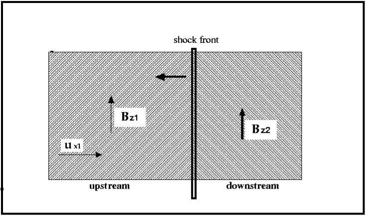
Figure 1: The simulation geometry.

The upstream and downstream conditions are related by the ideal MHD jump conditions for a relativistic, transverse, magnetosonic shock. These were derived by Kennel & Coroniti (1984), as expressed in the shock frame, and by Gallant et al. (1992) as expressed in the downstream frame. Quantities expressed in this latter frame are more convenient for purposes of direct comparison of the results of our numerical simulations with the theoretical expectations. Since the wall on the right of the simulation box is at rest, the $x$-component of the fluid velocity must vanish downstream of the shock. The downstream frame is therefore coincident with the computational observer’s frame and it is the frame in which all quantities that will enter the following discussion are measured. In this frame, the shock moves toward the left, with velocity $-c\beta_{shock}$. We assume the fluid upstream to be cold, $p_{1}\ll n_{1}mc^{2}$, where $p_{1}$ and $n_{1}$ are the proper pressure and density upstream, and to move at ultrarelativistic speed, with Lorentz factor $\gamma_{1}\gg 1$ and 4-velocity $cu_{1}\approx c\gamma_{1}$. For the fluid downstream, we assume the ideal ultrarelativistic equation of state to hold, with proper enthalpy $w_{2}\approx\Gamma p_{2}/(\Gamma-1)$. The adiabatic index $\Gamma$ would be equal to $4/3$ for an isotropic relativistic fluid. But in our analysis the particles’ momenta are restricted to the plane perpendicular to ${\bf B}$ therefore the appropriate value of $\Gamma$ is $3/2$, describing a 2-dimensional ultrarelativistic fluid.

After expressing the densities in terms of the simulation frame values $N=n\gamma$, the jump conditions reduce to:

$${N_{2}\over N_{1}} = {1+\beta_{\rm shock}\over\beta_{\rm shock}}\ ,$$ (1)

$$\left(1+\beta_{\rm shock}\right)N_{1}m\gamma_{1}c^{2}(1+\sigma) = \beta_{\rm shock}\left({p_{2}\over\Gamma-1}+{B_{2}^{2}\over 8\pi}\right)\ ,$$ (2)

$$\left(1+\beta_{\rm shock}\right)N_{1}m\gamma_{1}c^{2}(1+\sigma) = p_{2}+{B_{2}^{2}\over 8\pi}\ ,$$ (3)

$${B_{2}\over B_{1}} = {1+\beta_{\rm shock}\over\beta_{\rm shock}}\ ,$$ (4)

where we have used the definition of the magnetization parameter

$$\sigma={B_{1}^{2}\over 4\pi N_{1}mc^{2}\gamma_{1}}.$$

Using Eq. 3 and Eq. 4 to eliminate $p_{2}$ and $B_{2}$ from Eq. 2, one finds

$$\beta_{\rm shock}={1\over 2(1+1/\sigma)}\left\{\left({\Gamma\over 2}+{\Gamma-1\over\sigma}\right)+\left[\left({\Gamma\over 2}+{\Gamma-1\over\sigma}\right)^{2}+4\left(1-{\Gamma\over 2}\right)\left(1+{1\over\sigma}\right)\right]^{1/2}\right\}\ .$$ (5)

The jump in all quantities at the crossing of the shock front is then determined as a function of $\sigma$ and $\Gamma$. The density and magnetic field compression are determined through Eqs. 1 and 4, while the ratio between the thermal pressure downstream and the ram pressure upstream can be similarly expressed in terms of $\sigma$ and $\beta_{\rm shock}$ after manipulation of Eq. 2. One obtains:

$${kT_{2}\over m\gamma_{1}c^{2}}=\beta_{\rm shock}\left[1+\sigma\left(1-{1+\beta_{\rm shock}\over 2\beta_{\rm shock}}\right)\right]$$ (6)

The low and high $\sigma$ limits ($\sigma\ll 1$ and $\sigma\gg 1$, respectively) of Eqs. 1, 4, 5 and 6 are discussed extensively by Gallant et al. (1992), and the main result is that with increasing magnetization the fraction of upstream energy that goes into an increase of the magnetic pressure downstream becomes larger, at the expense of the particle thermal energy. In the following, we shall deal with the case of a plasma with $\sigma\approx 1$.

2.1 Numerical simulations of relativistic transverse shocks in a pure pair plasma

The results we show and discuss in the following refer to a simulation performed on a plasma with $\sigma_{-}=\sigma_{+}=2$, corresponding to $\sigma_{tot}=1$, and Lorentz factor upstream $\gamma_{1}=40$. The simulation grid was made of 1024 cells, each of size $\Delta x=r_{L}/10$, with $r_{L}$ being the particle Larmor radius based on the upstream $B$ field and flow Lorentz factor. The initial number of particles per cell was 32 for each species. The results are basically unchanged when $\Delta x$ is varied from $r_{L}/10$ to $r_{L}/5$, the number of cells between 512 and 2048, and the number of particles of each species per cell from 8 to 64. The time-step is $\Delta t=0.9\Delta x/c$ in all cases, in order to satisfy the Courant condition.

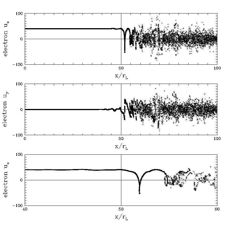
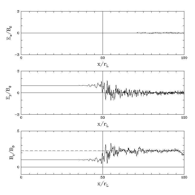
Figure 2: Plots on the left: The electron four-velocity as a function of position in the box. The x-coordinate is in units of $r_{L}$, the pair Larmor radius upstream. The shock front is located at $x_{s}/r_{L}\approx 50$. Top panel: x-component of the four velocity. Middle panel: y-component of the four-velocity. Bottom panel: a zoom of the top panel onto the region around the shock front. Plots on the right: The electromagnetic field as a function of position in the box. The x-coordinate is again in units of the pair Larmor radius upstream. Top panel: longitudinal component of the electric field. Middle panel: transverse component of the electric field. Bottom panel: the magnetic field.

As it was the case for the simulations performed by Gallant et al. (1992), we find in our simulation the presence of an electromagnetic precursor wave, propagating ahead of the shock, into the upstream medium, at essentially the speed of light. The results in the following figures refer to a time when the reverse shock has propagated far enough from the right wall of the simulation, so that edge effects (spurious oscillations due to the vicinity of the conducting boundary) do not affect the dynamics around the shock front, while the precursor has not reached the left boundary of the box yet.

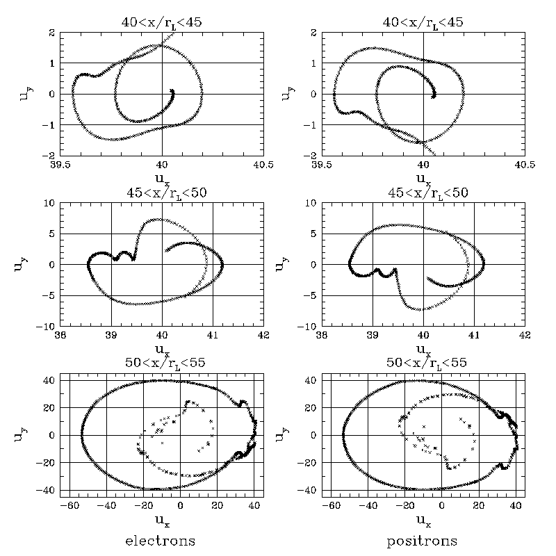
Figure 3: The electron (panels on the left) and positron (panels on the right) distribution in $u_{x}-u_{y}$ space in different regions around the shock front, as specified on top of each panel.

In Fig. 2 we show, on the left, the ($u_{x}-x$) and ($u_{y}-x$) sections of the electrons’ phasespace. The behavior of the positrons is completely analogous. The main thing to notice is the loop that develops at the crossing of the shock in the ($u_{x}-x$) plane, especially evident in the bottom panel. This is the initial reflection loop described by the soliton solution of Alsop & Arons (1988).

The particles’ four-velocities in the reflection region form distorted cold rings in momentum space, as shown in Fig. 3, so that one can expect cyclotron instability to develop, as expected from the uniform medium instability theory outlined in the Appendix with the ions omitted (see also Hoshino & Arons (1991)).

In Fig. 2 we also plot the different electromagnetic field components as a function of position. The longitudinal electric field always stays around zero with negligibly small oscillations. This is just what one expects due to the charge and mass symmetry, together with overall neutrality, leading to decoupling of the transverse from longitudinal extraordinary mode.

The transverse component of the electric field vanishes on average behind the shock, as predicted by ideal MHD, but of course there are oscillations due to the development of cyclotron instability in the pairs. The same behavior is seen in the magnetic field. The latter, after the first two main peaks, corresponding to the turning points of the first reflection loop, oscillates around the value computed from the jump conditions (Eqs. 4 and 5) for a plasma with $\sigma=1$ and $\Gamma=3/2$ (dashed curve in the plot).

Finally, in Fig. 4 we show the evolution of the pair distribution function at the crossing of the shock. It is apparent that no signs of non-thermal acceleration are observed. The distribution function progressively evolves towards a maxwellian for both species. The temperature of the maxwellian is in perfect agreement with the prediction of ideal MHD (Eq. 6): $T_{eff}=kT_{2}/m_{\pm}c^{2}\approx 0.4\ \gamma_{1}$.

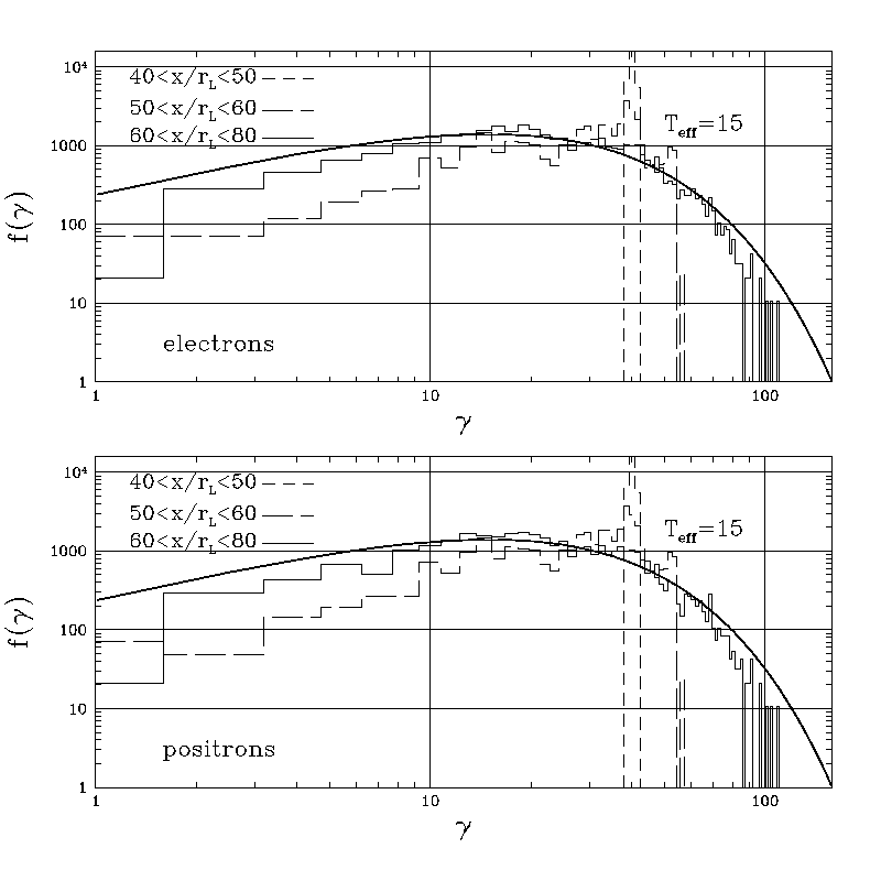
Figure 4: The evolution of the particle distribution after the crossing of the shock. The different line-types refer to particles extracted from different slices of the simulation domain as specified in the figure: short-dashed for particles at positions $40<x/r_{L}<50$, long-dashed for positions $50<x/r_{L}<60$ and solid for positions $60<x/r_{L}<80$. The top panel refers to electrons and the bottom one to positrons. In both cases $f(\gamma)$ is normalized to the particle number denisty upstream. The thick solid curve represents a 2-D relativistic maxwellian of temperature $T_{\rm eff}$ (see text).

2.2 Numerical Simulations of relativistic transverse shocks in $e^{-}-e^{+}-p$ plasmas: acceleration of electrons

We show that with protons present in the upstream flow, the downstream $e^{\pm}$ exhibit non-thermal heating, a.k.a. shock acceleration. We first tackle the problem of how the particle acceleration process is affected by the waves’ polarization.

In the following we discuss the results of two simulations in which a plasma with $\sigma_{-}=2$ and $\sigma_{i}=0.25$ is considered. The latter condition is realized in two different ways, first adopting a mass and number ratio between ions and electrons equal to 20 and 0.4 respectively (case A), and then using $m_{i}/m_{\pm}=40$ and $N_{i}/N_{-}=0.2$ (case B).

The simulation geometry is that in Fig. 1. In case A the simulation grid contains 2048 cells, each of size $r_{L1\pm}/10$, where $r_{L1\pm}=m_{\pm}c^{2}\gamma_{1}/eB_{1}$, while in case B the cell size is the same but the number of cells is doubled. In both cases the box contains more than 10 ion Larmor orbits and the number of particles per cell is 16. The initial plasma Lorentz factor is $\gamma_{1}=40$, but no dependence of the results on this parameter is expected as long as the condition $\gamma_{1}\gg 1$ is satisfied. As to the time-step, finally, this is taken to be $\Delta t=0.9\Delta x/c$, so that the Courant condition is ensured.

In Figs. 5-6 we show, on the left, the section ($u_{x}-x$) of the phase-space of the different species in the two different cases. The reverse shock is at around $x_{s}\approx 100r_{L}$ in Fig. 5 and $x_{s}\approx 200r_{L}$ in Fig. 6.

Comparing the left panels of the two figures, the first ion reflection loop is well defined in both cases, and the overall velocity profiles look very similar. At a closer look, however, one notices that in case B (Fig. 6) the spread in the electron four-velocity post-shock is larger than in case A, while the opposite happens for the positron velocities. This is a first signature of what we will find to be the most important difference between the two simulations.

Before discussing this point, however, let us briefly comment on the plots showing the electromagnetic field components in the two cases. First of all, in both cases, the presence of the electromagnetic precursor propagating ahead of the shock in the upstream medium is well evident. This wave is a purely transverse electromagnetic wave, as one can readily deduce from the absence of fluctuations in the longitudinal component of the electric field upstream of the shock. It is the same precursor as appears in magnetized shocks in pure pair plasmas (see previous section and also Gallant et al. (1992)), and is emitted by the quasi-coherent rings of $e^{\pm}$ reflected at the leading edge of the whole shock structure.

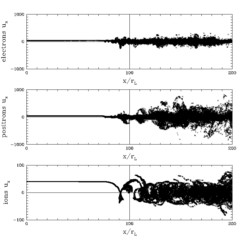
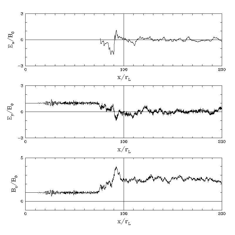
Figure 5: Left panel: The ($u_{x}-x$) section of the phase space of the different species for case A: electrons in the top panel, positrons in the middle panel and ions in the bottom panel. Right panel: The electromagnetic field components in the simulation labeled A: the fields are normalized to the upstream magnetic field intensity. In all plots the $x$-coordinate is in units of the pair gyration radius upstream.

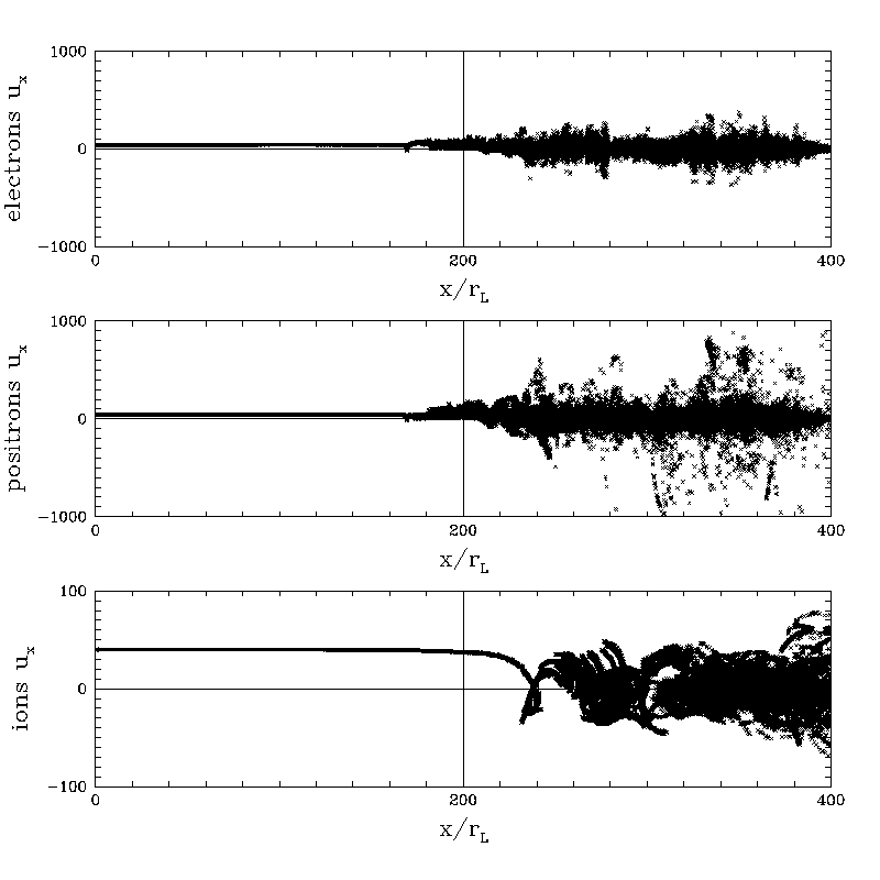
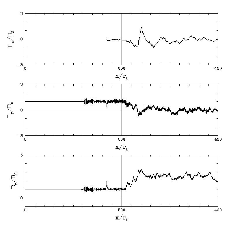
Figure 6: Same as Fig. 5 but for case B.

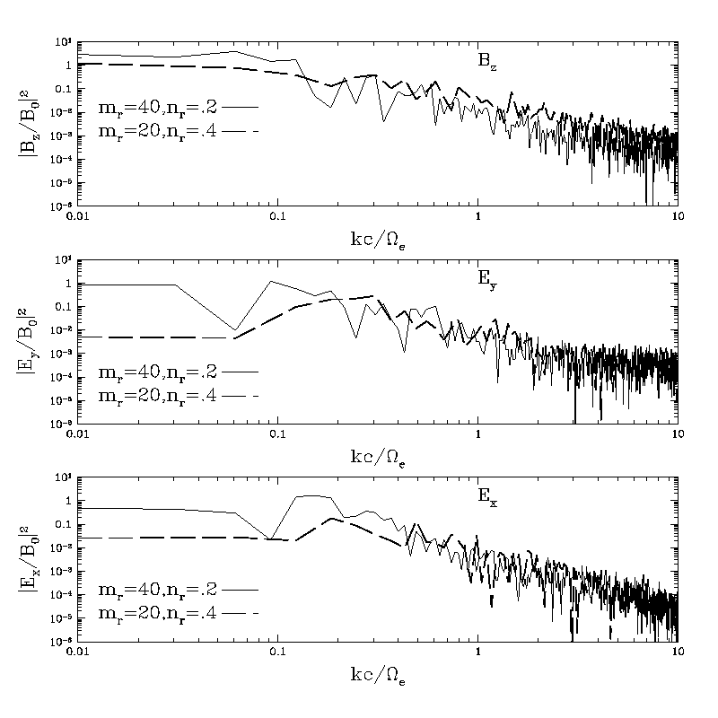
Figure 7: The downstream power spectra of the different electromagnetic field components, for case A (dashed curves) and case B (solid curves). The power spectrum is normalized to the value of the magnetic field upstream, while the wavenumbers are in units of $\Omega_{ce}/c$, with $\Omega_{ce}$ being the pairs’ Larmor frequency upstream.

As to the fields downstream, now the oscillations observed in the longitudinal component of the electric field are larger than in Fig. 2: due to the fact that the charge and mass symmetry of the pure pair plasma is broken by the presence of the ions, the transverse mode is partly longitudinal. The magnetic field oscillates around the enhanced post-shock value predicted by ideal MHD. The properties of the fields downstream are similar in the two cases we are now considering as it is clear from Fig. 7, where we compare the downstream power spectra extracted from the two simulations.

In both cases one finds that the power as a function of frequency can be approximated around the pair cyclotron frequency as a power law with index -2.

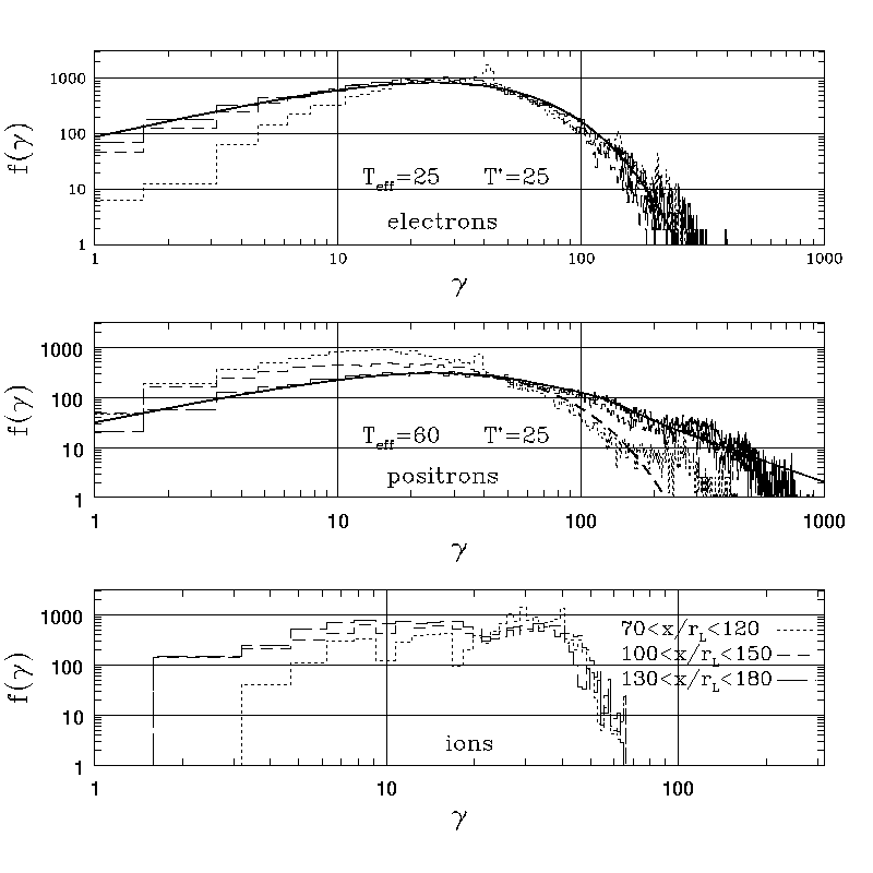
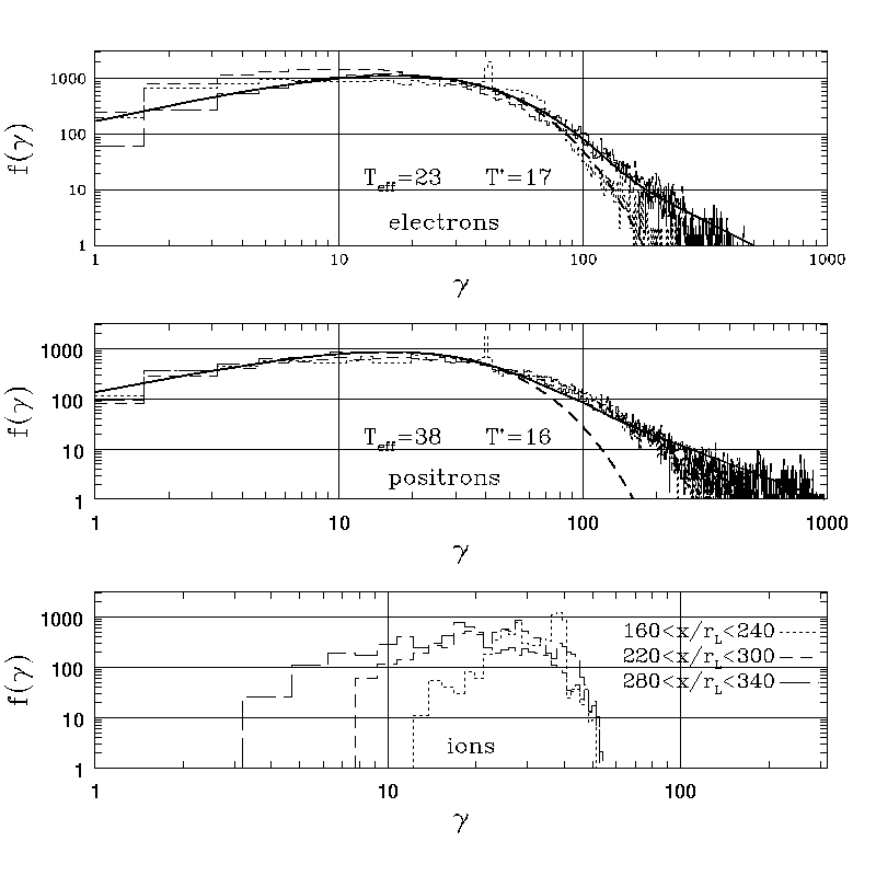
Figure 8: The postshock evolution of the distribution function of the different species, each normalized to the corresponding upstream density. The left panels refer to case A and the right panels to case B. The different line-types refer to different ranges of particle positions, as speciefied in the lower panel of each column. For electrons and positrons (upper and middle panels of each column) two fits of the distribution functions are presented together with the data. The thick dashed curve is a 2-D relativistic maxwellian with temperature $T^{\prime}$, while the thick solid curve is a maxwellian plus power-law fit (see text).

Finally we discuss the postshock evolution of the particle distribution functions. In Fig. 8 we plot for both cases (case A on the left and case B on the right) the distribution function of the different species within different regions behind the shock.

We observe, for all species, and in all cases, a progressive broadening of the distribution function with increasing distance from the shock front. However the details of the process are different between the different species and between the two simulations.

In case A, the energy release of the ions is quicker than in case B. One also sees, in the plots on the left, that a preferential heating of positrons occurs, as shown by the effective temperatures of the different species (value of $T_{\rm eff}$ reported in the plots). Moreover, positrons are not only heated but also non-thermally accelerated, since the energy excess is found in the form of a well developed high energy suprathermal tail.

In case B, one still observes hotter positrons than electrons, but the difference between the effective temperatures of the two species is smaller. The final value of $T_{\rm eff}$ is, for both species, smaller than in case A, and the suprathermal positron tail is reduced, despite being still evident, while signs of electron acceleration are found for the first time.

We fit the final distribution functions of the pairs (thick solid curves in the top and middle panels of Fig. 8) with a function $N(\gamma)$ given by the superposition of a 2-D relativistic maxwellian plus a power-law tail, with the latter exponentially cut-off at low energies:

$$\frac{N_{\pm}(\gamma)}{N_{1\pm}}={f\over T^{\prime}(T^{\prime}+1)}\gamma\exp{\left[-{\gamma-1\over T^{\prime}}\right]}+N_{t}\left({\gamma\over\gamma_{m}}\right)^{-\alpha}\left\{1-\exp{\left[-\left({\gamma-1\over\gamma_{m}}\right)^{r}\right]}\right\}\ .$$ (7)

In Eq. 7, $N_{1}$ is the upstream density of the species considered and $T^{\prime}=T/m_{\pm}c^{2}$, $\alpha$ and $r$ are the power-law indices of the suprathermal tail and of the cut-off, respectively, and, finally, $\gamma_{m}$ is the Lorentz factor at which the power-law tail is cut-off.

The best fit function is plotted in each of the relevant panels of Fig. 8 as a thick solid curve, while the thick dashed curve represents a maxwellian of temperature $T^{\prime}\equiv T/m_{\pm}c^{2}$. The curves we plot are defined by using for the parameters appearing in Eq. 7 the values listed in Table 1. In the last row of the same table we report the acceleration efficiency in terms of energy, $\eta$. This is computed as the ratio between the energy density of $e^{-}$ and $e^{+}$ in the suprathermal tail of the distribution, $U_{nt\pm}$ and the total upstream flow energy density $U_{tot}$:

$$\eta_{\pm}=U_{nt\pm}/U_{tot}\ ,$$ (8)

with

$$U_{tot} = (\gamma_{1}-1)c^{2}\left[N_{1i}m_{i}+m_{\pm}(N_{1-}+N_{1+})\right]+\frac{B_{1}^{2}}{8\pi}(1+\beta_{1}^{2})$$ (9)

$$= (\gamma_{1}-1)m_{\pm}c^{2}N_{1-}\left[2+\left(\frac{m_{i}}{m_{\pm}}-1\right)\frac{N_{1i}}{N_{1-}}+\sigma_{-}\right]\ ,$$

and $U_{nt\pm}$ computed as the integral of the second term in Eq. 7 multiplied by $m_{\pm}\gamma c^{2}$:

$$U_{nt\pm}=N_{1\pm}m_{\pm}c^{2}\gamma_{m}^{2}N_{t}\int_{1}^{\gamma_{max}/\gamma_{m}}dx\ x^{1-\alpha}\ \left\{1-\exp\left[-\left(x-\frac{1}{\gamma_{m}}\right)^{r}\right]\right\}\ .$$ (10)

In the latter equation we see that a parameter $\gamma_{max}$ appears, that refers to the maximum Lorentz factor up to which particles are accelerated. The theoretical upper limit for $\gamma_{max}$ within the framework of the proposed acceleration mechanism is $\gamma_{max}^{th}=m_{i}/m_{\pm}\gamma_{1}$, i.e. the pairs cannot be accelerated up to energies exceeding the ions’ energy upstream.

Simulation parameters
	case A		case B
$m_{i}/m_{\pm}$	$20$		$40$
$N_{i}/N_{-}$	$0.4$		$0.2$
$U_{i}/U_{tot}$	$0.69$		$0.68$
$U_{i}/U_{-}$	$8$		$8$
Downstream $e^{\pm}$ distribution parameters
	electrons	positrons	electrons	positrons
f	1	0.6	0.92	0.8
T’	25	25	17	16
$\gamma_{m}$	-	100	80	80
$N_{t}$	0	$3\times 10^{-3}$	$1\times 10^{-3}$	$2\times 10^{-3}$
$\alpha$	-	1.7	2.2	1.8
$r$	-	4	4	4
$\gamma_{max}/\gamma_{max}^{th}$	-	1	0.3	0.75
$\eta$ [%]	$<2$	20	3	11

Table 1: In the upper part of the table we report the values of the paramaters with which the simulation was performed: mass ratio between the species; number ratio between ions and electrons; fraction of the total upstream energy density carried by the ions; ratio between the ions’ and electrons’ energy density upstream. In the lower part of the table, we report the best fit values of the parameters in Eq. 7, describing the electrons’ and positrons’ distribution downstream. In the bottom line we report the energy acceleration efficiency for the pairs, estimated (Eq. 8) as the percentage of the total upstream energy density $U_{tot}$ converted into non-thermal $e^{\pm}$ in each case.

The results presented in this section are summarized as follows. When the ions are only 20 times more massive than the pairs and 40% of the total number of positive charges, only positron acceleration is observed. When a different simulation plasma is considered, with the same amount of energy in baryons as before, but given to a smaller fraction by number of more massive ions, the fraction of energy that is converted into accelerated positrons is found to be smaller; their spectrum is steeper and also the maximum Lorentz factor reached is lower. At the same time, however, signs of electron acceleration start appearing, although the efficiency of this latter process is lower compared to that of positron acceleration; the $e^{-}$ spectrum is softer and their maximum Lorentz factor smaller than that of $e^{+}$. It is important to notice that while the results concerning simulation A are in agreement with those of Hoshino et al. (1992), the simulation B is the first of this kind in the literature to show traces of electron acceleration, thanks to the larger mass ratio and correspondingly lower number ratio between the ions and the pairs employed. This confirms the role of the wave polarization in the acceleration process.

2.3 Relativistic transverse shocks in $e^{-}-e^{+}-p$ plasmas: $m_{i}/m_{\pm}=100$

We now analyze how the situation changes increasing the mass-ratio between the ions and the pairs to $m_{i}/m_{\pm}=100$.

In Fig. 10 we show the energy distribution of the particles at different positions behind the shock, for three simulations with $m_{i}/m_{\pm}=100$ and $N_{i}/N_{-}$ varying between 0.05 and 0.2. In all simulations we employed a box of 10240 cells and the number of particles of each species per cell was 12. The size of each cell was $\Delta x=r_{Le}/10$, with $r_{Le}$ being the pair Larmor radius upstream. The time-step was $\Delta t=0.9\Delta x/c$.

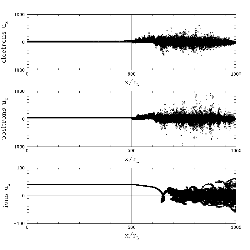
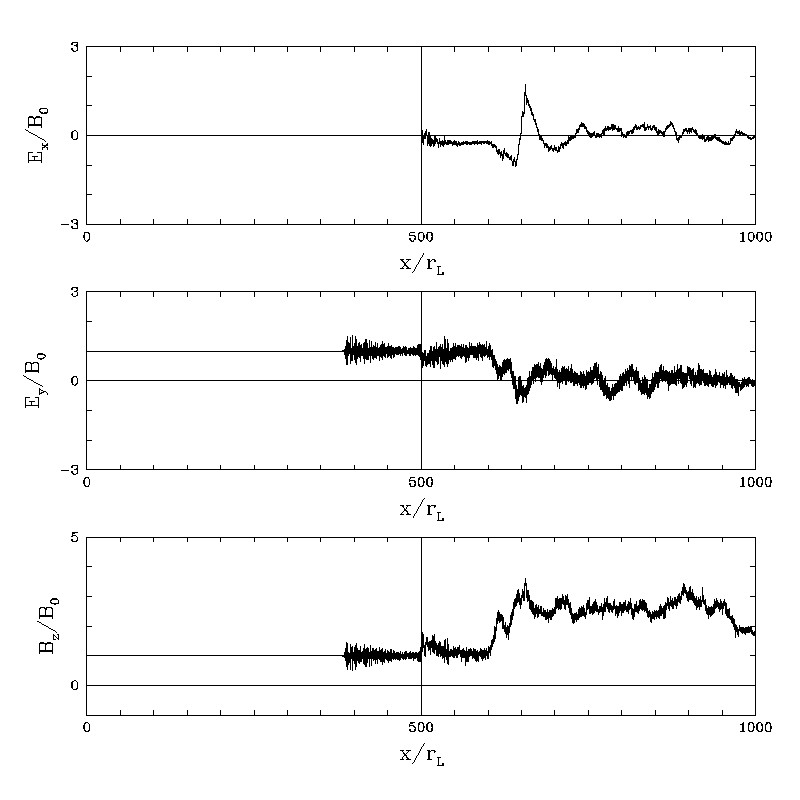
Figure 9: Left panel: The ($u_{x}-x$) section of the phase space of the different species for the simulation with $m_{i}/m_{\pm}=100$ and $N_{i}/N_{-}=0.1$. Right panel: The electromagnetic field components, normalized to the upstream magnetic field intensity, for the same simulation. In all plots the $x$-coordinate is in units of the pair gyration radius upstream.

The snapshot of the simulation to which the plots in Fig. 10 refer was taken when the shock position was around $x_{s}/r_{Le}=500$. The particle distribution in velocity space and the electromagnetic field components are shown in Fig. 9 for the case $N_{i}/N_{-}=0.1$. From comparison of the left panel of this figure, with the left panels of Figs. 5 and 6 one sees that the electrons show an increasingly large spread in their velocity distribution with decreasing $N_{i}/N_{-}$. This feature is made more quantitative by Fig. 10 and Table 2, where simulations performed with the same value of the mass ratio ($m_{i}/m_{\pm}=100$) but different fractions of ions are compared.

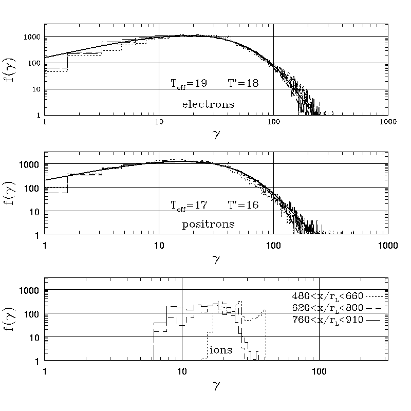
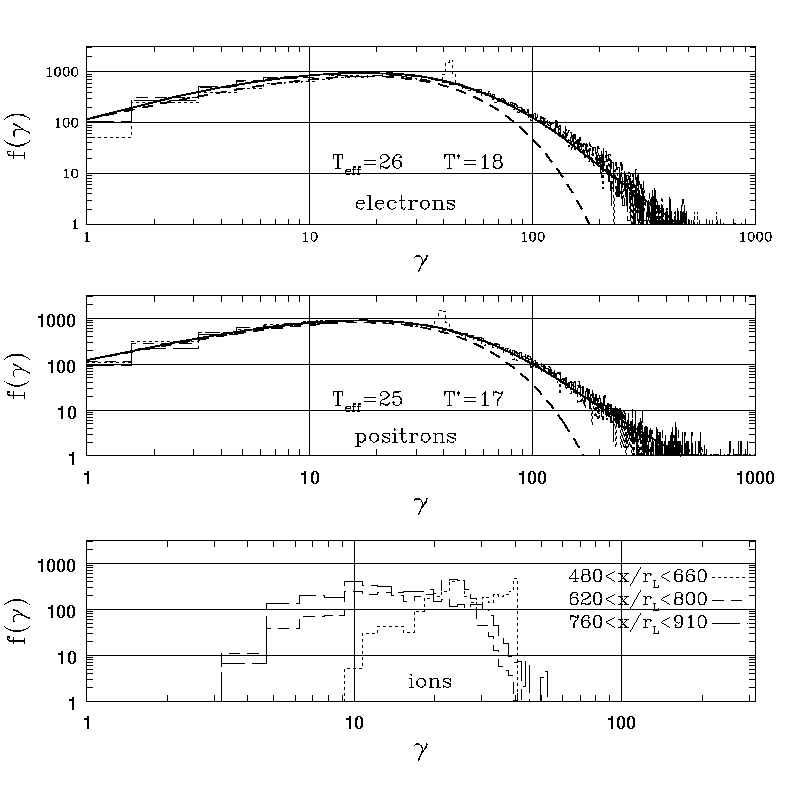
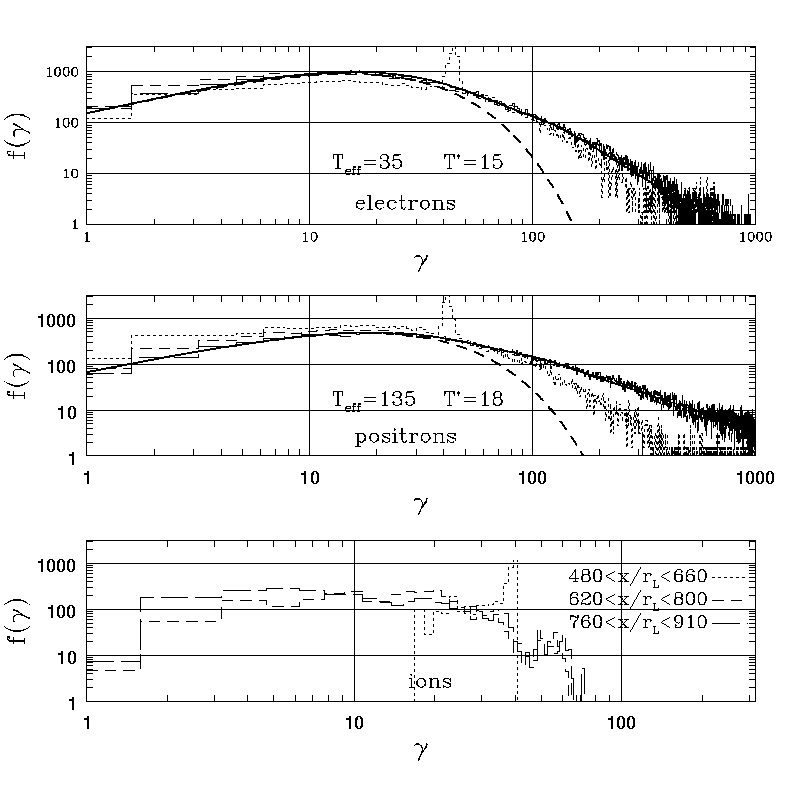
Figure 10: The postshock evolution of the distribution function of the different species, each normalized to the relative upstream density. Left column : $N_{i}/N_{-}=0.05$. Middle column: $N_{i}/N_{-}=0.1$. Right column: $N_{i}/N_{-}=0.2$. The notation is the same as for Fig. 8, with the thick solid curve representing a fit of the distribution with the function described by Eq. 7. The best fit values of the parameters are those in Table 2.

Simulation parameters
$m_{i}/m_{\pm}=100$
$N_{i}/N_{-}$	$0.05$		$0.1$		$0.2$
$U_{i}/U_{tot}$	$0.56$		$0.72$		$0.84$
$U_{i}/U_{-}$	$5$		$10$		$20$
Downstream $e^{\pm}$ distribution parameters
	electrons	positrons	electrons	positrons	electrons	positrons
f	0.97	0.97	0.7	0.7	0.65	0.5
T’	18	16	18	17	15	18
$\gamma_{m}$	100	100	100	90	100	85
$N_{t}$	$3.5\times 10^{-4}$	$3.7\times 10^{-4}$	$2.2\times 10^{-3}$	$2.3\times 10^{-3}$	$3.2\times 10^{-3}$	$4.2\times 10^{-3}$
$\alpha$	3.5	3.5	3.2	2.9	2.7	1.6
$r$	4	4	3	3	3	3
$\gamma_{max}/\gamma_{max}^{th}$	0.15	0.3	0.2	0.4	0.3	0.8
$\eta$ [%]	$0.9$	$1$	$5$	$5$	$5$	$27$

Table 2: The table refers to simulations employing a mass-ratio of 100 between the ions and the pairs and number ratios $N_{p1}/N_{e1}$ varying between 0.05 and 0.2. In the upper part of the table we report the values of the paramaters with which each simulation was performed: number ratio between ions and electrons; fraction of the total upstream energy density carried by the ions; ratio between the ions’ and electrons’ energy density upstream. In the lower part of the table, we report the best fit values of the parameters in Eq. 7, describing the electrons’ and positrons’ distribution downstream. In the bottom line we report the energy acceleration efficiency for the pairs, estimated (Eq. 8) as the percentage of the total upstream energy density $U_{tot}$ converted into non-thermal $e^{\pm}$ in each case.

It is apparent from Fig. 10 that efficient acceleration of both electrons and positrons is found for $N_{i}/N_{-}\geq 0.1$. A very large acceleration efficiency is observed in the case when $N_{i}/N_{-}=0.2$, for both species of particles: 50% of the positrons and 35% of the electrons are found in the suprathermal tail of the distribution in this case, with an energy acceleration efficiency that almost reaches 30% for positrons. The ratio between the efficiencies of electron and positron acceleration is found to be similar to that in simulation B ($m_{i}/m_{\pm}=40$, $N_{i}/N_{-}=0.2$) of the previous section, so that the conclusion we derive is that this is strictly related to the degree of neutrality of the pair plasma, which affects the polarization of the waves.

The percentage of energy in suprathermal particles is drastically reduced when the number of ions is reduced from $N_{i}=0.2N_{-}$ to $N_{i}=0.1\ N_{-}$ and as a consequence the energy ratio is halved. At the same time, the pair plasma becomes closer to neutral and the behavior of the different species of light particles becomes increasingly similar. For $N_{i}=0.1\ N_{-}$ the energy content of the high energy tails of the distributions of the two species is the same, and the slopes of the suprathermal power laws become similar, though steeper than when the ions are twice as many.

If $N_{i}/N_{-}$ is decreased further by a factor of two the acceleration efficiency is reduced by a factor of 5 for both species and the power law indices increase further, becoming exactly the same.

2.4 Relativistic transverse shocks in $e^{-}-e^{+}-p$ plasmas: Effect of Finite Upstream Temperature

The results described in §2.2 and §2.3 assumed the upstream flow to be completely cold, i.e., to have zero momentum dispersion. The linear theory outlined in §A.1 suggests that if the upstream flow is warm enough, magnetosonic waves at high harmonics of the ion cyclotron frequency will be absent in the medium behind the shock in the pairs, thus reducing the efficiency of injection of pairs into the acceleration mechanism. The lack of the harmonics above $n=u_{1}/\Delta u$, where $\Delta u$ is the momentum dispersion of the upstream ion flow, means that the minimum energy that can be accelerated by cyclotron resonance is $m_{\pm}c^{2}\gamma_{min}=(m_{i}c^{2}/M_{s})\gamma_{1}$, if $M_{s}=u_{1}/\Delta u<m_{i}/m_{\pm}$. Thus the suprathermal tail starts farther and farther out on the Maxwellian tail of the pairs, for smaller and smaller $M_{s}$, thus reducing the acceleration efficiency (and steepening the power law part of the spectrum). The maximum energy possible is still set by resonance with the fundamental, but now there are many fewer such particles.

The simulations whose results are shown in the following were performed assuming gaussian functions to describe the particles’ distribution upstream of the shock:

$$f(u_{x},u_{y})=\frac{1}{\pi\Delta u^{2}}\exp\left[-\frac{(u_{x}-u_{1})^{2}}{\Delta u^{2}}\right]\ \exp\left[-\left(\frac{u_{y}}{\Delta u}\right)^{2}\right].$$ (11)

$M_{s}\equiv u_{1}/\Delta u$ is the relativistic flow sonic Mach number as defined in the linear instability theory.

All three species of particles were injected in the box according to the distribution function in Eq. 11, with $u_{1}$ corresponding to a Lorentz factor $\gamma_{1}=40$ and $\Delta u=0.1\ u_{1}$. The mass ratio between the ions and the pairs was taken to be $m_{i}/m_{\pm}=100$ and two different simulations were performed, corresponding to $N_{i}/N_{-}=0.1$ and $N_{i}/N_{-}=0.2$. Except for the substitution of a Dirac $\delta$ with a gaussian as the function describing the particles distribution, the simulation set-up is exactly the same as that described in §§2.3, i.e. same number of cells and of particles per cell, same cell-size (in units of the mean pair Larmor radius upstream) and time-step.

Fig. 11 is a snap-shot of the simulation with $N_{i}/N_{-}=0.1$, taken when the shock front is at $x/r_{L}\simeq 500$. In this figure we plot the particles’ phase-space and the electromagnetic fields in the simulation for a direct comparison with those in Fig. 11, which referred to the same incoming plasma taken to be completely cold.

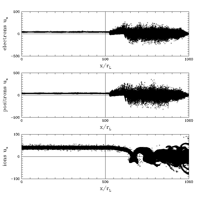
Figure 11: Left panel: The ($u_{x}-x$) section of the phase space of the different species for a simulation with $m_{i}/m_{\pm}=100$ and $N_{i}/N_{-}=0.1$. The particle distribution function upstream of the shock is described by Eq. 11 with $u_{1}\simeq 40$ and $\Delta u=0.1\ u_{1}\;(M_{s}=u_{1}/\Delta u=10)$. The shock front is at $x/r_{L}\simeq 500$. Right panel: The electromagnetic field components, normalized to the upstream magnetic field intensity, for the same simulation. In all plots the $x$-coordinate is in units of the mean (corresponding to $\gamma_{1}$) pair gyration radius upstream.

From the comparison of Fig. 11 with Fig. 9 it is immediately apparent that the maximum pair energy downstream is reduced when a spread in the particle velocities upstream is introduced.

The differences are even more evident from the comparison between Fig. 10 and Fig. 12. In the latter we plot the particle distribution functions as extracted from slices of the simulation at different distances from the shock front. The left and right panels refer to the case when $N_{i}/N_{-}=0.1$ and $N_{i}/N_{-}=0.2$ respectively, and hence should be compared to the middle and right panel in Fig. 10. The notation is the same as for that figure.

Simulation parameters
	$m_{i}/m_{\pm}=100$		$\Delta u/u_{0}=0.1$
$N_{i}/N_{-}$	$0.1$		$0.2$
$U_{i}/U_{tot}$	$0.72$		$0.84$
$U_{i}/U_{-}$	$10$		$20$
Downstream $e^{\pm}$ distribution parameters
	electrons	positrons	electrons	positrons
f	0.85	0.8	0.6	0.6
T’	20	20	19	19
$\gamma_{m}$	120	110	120	100
$N_{t}$	$10^{-3}$	$2\times 10^{-3}$	$3\times 10^{-3}$	$4\times 10^{-3}$
$\alpha$	4.5	4.	4.	3.3
$r$	4	4	4	4
$\gamma_{max}/\gamma_{max}^{th}$	0.09	0.1	0.15	0.65
$\eta$ [%]	2.5	4	4	4

Table 3: The table refers to simulations employing a mass-ratio of 100 between the ions and the pairs and a finite temperature upstream: $\Delta u/u_{0}=0.1$ (plots in Fig. 12). In the upper part of the table we report the values of the paramaters with which each simulation was performed: number ratio between ions and electrons; fraction of the total upstream energy density carried by the ions; ratio between the ions’ and electrons’ energy density upstream. In the lower part of the table, we report the best fit values of the parameters in Eq. 7, describing the electrons’ and positrons’ distribution downstream. In the bottom line we report the energy acceleration efficiency for the pairs, estimated (Eq. 8) as the percentage of the total upstream energy density $U_{tot}$ converted into non-thermal $e^{\pm}$ in each case.

The particle acceleration efficiency is reduced with respect to the case when the upstream plasma was taken to be completely cold. As one can see by comparing the values of the parameters in Table 3 with those in Table 2, for both values of $N_{i}/N_{-}$, the fraction of energy carried by suprathermal particles is smaller and the power-law index of the suprathermal tail is steeper.

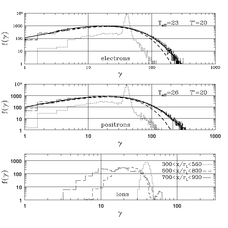
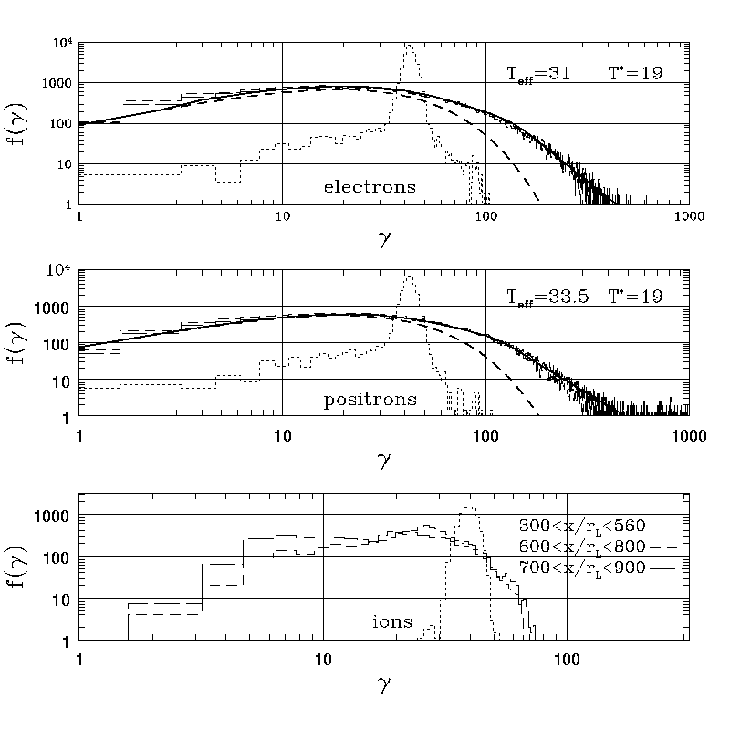
Figure 12: The postshock evolution of the distribution function of the different species, each normalized to the relative upstream density. Left column : $N_{i}/N_{-}=0.1$. Right column: $N_{i}/N_{-}=0.2$. The notation is the same as for Fig. 10, with the thick solid curve representing a fit of the distribution with the function described by Eq. 7. The best fit values of the parameters are those in Table 3.

The resonance condition for absorption of an ion cyclotron wave by an electron or positron requires that $n\Omega_{ci}=\Omega_{c\pm}$. Thermal dispersion $\Delta u/u_{1}>m_{\pm}/m_{p}$ in the upstream ions prevents growth for harmonic number $n>M_{s}=u_{1}/\Delta u$, which cuts the efficiency of generation of a non-thermal tail to the pairs’ momentum distributions.

3 Discussion and Conclusions

In accord with previous results (Langdon et al. (1988); Gallant et al. (1992)), we find full thermalization in pure $e^{-}-e^{+}$ shocks. The reason is the rapid reabsorption of waves at and above the upper hybrid frequency $\Omega_{UH\pm}$, which causes the shock to behave as if it were collisional - rapid emission of the EM waves by the relativistic cyclotron instability at the particle reflection front, with rapid reabsorption of the waves, and exchange of real photons, is a mechanism just as capable as the exchange of virtual photons in Coulomb collisions in producing local thermodynamic equilibrium. The conclusion, that pure pair shocks yield relativistic Maxwellians in the downstream medium, is not limited to the one-dimensionality of our model, as is shown elsewhere in 3D simulations by Spitkovsky and Arons (in preparation). Those simulations show that at sufficiently low $\sigma$ ($\sigma<10^{-3}$ is low enough), the relativistic Weibel instability (e.g., Yoon and Davidson (1987)) takes over from cyclotron instability in the pairs as the deceleration and thermalization mechanism of the shock wave, even when the background magnetic field is fully transverse to the flow. The physical reasons for this result are discussed in detail elsewhere, in the context of the 3D results. However, the essence is that the magnetic fields generated by the Weibel instability in an unmagnetized shock saturate in a tangled network of tangled magnetic filaments (Milosavljevic & Nakar (2006)), taking a distance $l_{therm}\sim 25c/\omega_{p1}$. These filaments scatter and thermalize the incoming particles. Since $l_{therm}/r_{L1\pm}\sim 25\sqrt{\sigma_{1\pm}}$, Weibel based thermalization (a multi-diemensional effect) controls the shock structure for $\sigma_{1\pm}<0.002$. For larger magnetizations, the cyclotron effects studied here dominate, somewhat modified by mild crinkling of the shock front.

In the shock wave, the incoming flow continuously injects cold ($M_{s}\gg 1$) ions into the pair plasma, the latter being already heated by the leading shock in the pairs alone. These freshly injected cold ions efficiently produce high harmonic waves which are cyclotron resonant with the pairs, even though the heated ions that are found further downstream from the pair shock do not efficiently radiate high harmonic waves. Magnetic reflection at the shock front produces a continuous supply of cold gyrating ions, thus ensuring energy transfer from the ions to the non-thermal pairs in the downstream medium, different from what is the case in the analogous initial value problem in a uniform medium.

When the ion density is a small fraction of the pair density, non-thermal acceleration becomes symmetric between electrons and positrons. It also becomes less efficient, leading to steeper power-law slopes in the non-thermal part of the spectrum. As shown in Fig. 10, the spectra take a Maxwellian form up to energies around $E_{\pm}\approx\gamma_{1}m_{\pm}c^{2}$, then have a power law form at higher energies. The energy above which the power law distribution sets in, and the slope, depend on $N_{i}/N_{\pm}$. Thus, apparent universality (if it exists) of power law spectra in synchrotron sources where relativistic shocks are inferred to play a role in non-thermal accleration would be a consequence of universality in the composition of the upstream flow, expressed as the ratio $N_{1i}/N_{1\pm}$, if the cyclotron resonance mechanism described here really is the dominant non-thermal heating process and if all relativistic shocks are sufficiently close to the transverse geometry studied here.

At present, nothing has been published on the full 3D structure of these shocks. Our expectation is that the 3D structure of electron-positron-ion transverse shocks will show a transition to unmagnetized physics at a low value of $\sigma_{1,total}$. The value of this transition magnetization is quite uncertain, since current neutralization of the ion filaments formed by the Weibel instability by electron return currents (Lyubarsky & Eichler (2006)) may greatly increase the thermalization length, thus giving more room in $\sigma$ space for cyclotron dynamics to ultimately mediate the shock structure. These issues are under investigation.

Relativistic flows that get their energization from Poynting losses from compact objects (possibly all in our list of pulsar winds, microquasar, AGN and GRB jets) may well be in this category, since the pair and ion content may both be set by the underlying electrodynamics of the compact objects (rotating neutron star, magnetized disk.) Quantification of how close shocks have to be to transverse requires consideration of a wider range of shock geometries. Investigation of other non-thermal heating mechanisms, such as Diffusive Shock Acceleration and magnetic pumping, require higher dimensional simulations. Spitkovsky and Arons (in preparation) address both of these issues.

In the shocks, the relative proportion of electron versus positron acceleration follows the ion to pair density, as expected from the changes in wave polarization inferred from the linear theory.

Our study of the shock acceleration process confirms, therefore, the results found by Hoshino et al. (1992), extending them to a higher mass ratio. Also confirmed is the expectation that signs of electron acceleration would be found if one could consider a plasma that contained the same amount of upstream flow energy given to a smaller fraction of ions. The overall evolution of the particles is consistent with resonant cyclotron absorption of magnetosonic waves by the pairs, whose frequencies are harmonics of the ion cyclotron frequency, being the main process providing non-thermal acceleration. Magnetic reflection of the upstream ions in the shock front sets up the unstable ion cyclotron motion which causes the wave emission. The non-thermal acceleration efficiencies and power law indices of the particle spectra are shown, as a function of the basic governing parameter $N_{i}/N_{-}$, in Table 2, when the upstream flow is cold. The reduction of the acceleration efficiency for a single value of the Mach number $M_{s}=10\ll m_{i}/m_{\pm}=100$, with results summarized in Table 3, shows the strong effect of large upstream momentum dispersion in the upstream flow. Equivalently, the absorption of ion cyclotron waves in the shock structure by the pairs is a strong non-thermal acceleration mechanism when the upstream flow is quite cold ($M_{s}>m_{i}/m_{\pm}$), as results from adiabatic expansion in relativistic outflows from compact objects.

We conclude by pointing out an interesting feature of this acceleration mechanism. The acceleration efficiency and the spectral form of the accelerated particles depend on the composition of the flow upstream of the shock. That composition depends on the source of the relativistic flow within which the shock wave occurs. Relativistic flows of the type considered here are thought to be the consequence of magnetized wind and jet acceleration by compact objects, and pair creation within and near such objects. These properties are the result of the compact objects’ electrodynamics, which constrains some aspects of the outflowing plasma composition to particular values - for example, in pulsars and magnetars, the ion flux is constrained to be the Goldreich-Julian value. Thus, one might expect a correlation between the radiative emission properties of the shocked flow and the emission properties of the underlying compact object, as appears to be the case in the X-ray emission from pulsar wind nebulae and the spectra of the pulsed X-ray emission from the pulsars driving those nebulae (Gotthelf (2003)).

Appendix A Relativistic Cyclotron Instability of Ring Distributions in a Uniform Magnetized $e^{+}-e^{-}-p\,$ plasma

We consider an overall neutral $e^{+}-e^{-}-p\,$ plasma uniformly distributed in space and permeated by a uniform magnetic field. The initial distribution of the plasma in momentum space is described as rings, with all species gyrating in the background magnetic field with the same Lorentz factor, $\gamma_{+}=\gamma_{-}=\gamma_{p}$. For most of the work in this section, we assume that all the species are cold, that is, have no dispersion around their gyration momenta. In preparation for the shock studies described in §2, we also briefly describe some results of the linear instability theory when the ions gyrate with a small momentum dispersion in a relativistically hot pair plasma.

Cold ring distributions are known to be unstable to cyclotron emission and the growth-rate of the instability scales proportionally to the particles’ cyclotron frequency. Hence, in the situation we are presently considering the process of relaxation of the particles’ distribution functions will show two different stages.

Initially, the pairs, whose gyration frequencies are much larger than those of the ions, will undergo cyclotron instability and tend to thermalize through emission and absorption of relativistic cyclotron waves. During this stage, the ions form a static uniform neutralizing background: they cannot interact efficiently with the waves produced by the pairs, which are too high frequency, and therefore their distribution is expected to be left nearly unchanged while the pairs relax. Only at later times the ions will develop the same instability, with the delay determined by the difference in the Larmor frequencies of the lighter and heavier particles.

In the case of a plasma with about equal amount of energy carried by light particles and magnetic fields ($\sigma_{-}\simeq\sigma_{+}\simeq 1$), the time-scale for the cyclotron instability in the pairs to reach saturation turns out to be of order a few tens of gyration periods, while it is shorter for lower magnetization (see Hoshino & Arons (1991)). Hence, if one considers, as we shall do in the following, a plasma with magnetization $\sigma\lower 3.44444pt\hbox{$\;\buildrel<\over{\sim}\;$}1$, for high enough mass ratios, the expectation is that the instability of the pairs will have reached saturation, and they will have already almost completely thermalized, before the ion cyclotron instability sets in.

A.1 Linear theory of the ion cyclotron instability

The ion distribution function is described by:

$$f_{i}(u_{\perp},u_{\parallel})={1\over 2\pi u_{0}}\delta(u_{\perp}-u_{0})\delta(u_{\parallel}),$$ (A1)

where $u$ is the particle four-velocity ($u=\gamma\beta$, with $\gamma=1/\sqrt{1-\beta^{2}}$ being the particle Lorentz factor), $u_{0}$ is the initial value of $u$ and the symbols $\parallel$ and $\perp$ are with respect to the magnetic field direction. We assume the magnetic field aligned with the z-axis of a cartesian system of coordinates ${\bf B}=B{\bf e}_{z}$. Since we are interested in the particles’ cyclotron emission the waves we are going to consider will have both the electric field and wave vector perpendicular to the magnetic field direction (extraordinary mode). If we assume ${\bf k}=k{\bf e}_{x}$ the dispersion relation can be written as:

$${c^{2}k^{2}\over\omega^{2}}=\varepsilon_{yy}-{\varepsilon_{xy}\varepsilon_{yx}\over\varepsilon_{xx}}\ .$$ (A2)

The general expression for the dielectric tensor in a uniform magnetized plasma can be found, for example, following the theory in the book by Krall & Trivelpiece (1973) (see also Hoshino & Arons (1991)). We mentioned above that when the ion instability is still in its early phases, the pairs will have already exhausted their free energy. This fact leads us to expect the fluid approximation to appropriately describe the pairs’ contribution to the propagation characteristics of the waves whose growth is stimulated by the ions. We will therefore describe the pairs’ response as that of a relativistically hot fluid with effective temperature $T_{\pm}$ ($k_{B}T_{\pm}=P_{\pm}/N_{\pm}$ where $P_{\pm}$ is the pressure and $N_{\pm}$ the number density) and adiabatic index $\Gamma$. The latter would be $\Gamma=4/3$ for a 3D relativistic plasma and $\Gamma=3/2$ for a 2D relativistic plasma: we confine our attention to the 2D case, since our spatially 1D simulations do not heat the plasma in the magnetic field direction.

The relevant components of the dielectric tensor will then be given by:

$$\varepsilon_{xx}=1+2\pi\sum_{n=-\infty}^{\infty}{n^{2}\over\nu_{i}^{2}}{\gamma_{0}^{2}\over\sigma_{i}\alpha_{i}^{2}}\int du_{\parallel}du_{\perp}{\partial f_{i}\over\partial u_{\perp}}\ {(J_{n}(\alpha_{i}u_{\perp}/\gamma_{0}))^{2}\over(\sqrt{1+u_{\perp}^{2}}/\gamma_{0}-n/\nu_{i})}+$$

$$+\left({1\over\sigma_{-}}+{1\over\sigma_{+}}\right){1\over(1-\nu_{e}^{2}+(\Gamma-1)\alpha_{e}^{2})}\ ,$$ (A3)

$$\varepsilon_{xy}=-\varepsilon_{yx}=2\pi{\it i}\sum_{n=-\infty}^{\infty}{n\over\nu_{i}^{2}}{\gamma_{0}\over\sigma_{i}\alpha_{i}}\int du_{\parallel}du_{\perp}u_{\perp}{\partial f_{i}\over\partial u_{\perp}}\ {J_{n}(\alpha_{i}u_{\perp}/\gamma_{0})\ J_{n}^{\prime}(\alpha_{i}u_{\perp}/\gamma_{0})\over(\sqrt{1+u_{\perp}^{2}}/\gamma_{0}-n/\nu_{i})}+$$

$$+{{\it i}\over\nu_{e}}\left({1\over\sigma_{+}}-{1\over\sigma_{-}}\right){1\over(1-\nu_{e}^{2}+(\Gamma-1)\alpha_{e}^{2})}\ ,$$ (A4)

$$\varepsilon_{yy}=1+2\pi\sum_{n=-\infty}^{\infty}{1\over\nu_{i}^{2}}{1\over\sigma_{i}}\int du_{\parallel}du_{\perp}u_{\perp}^{2}{\partial f_{i}\over\partial u_{\perp}}\ {(J_{n}^{\prime}(\alpha_{i}u_{\perp}/\gamma_{0}))^{2}\over(\sqrt{1+u_{\perp}^{2}}/\gamma_{0}-n/\nu_{i})}+$$

$$+\left({1\over\sigma_{-}}+{1\over\sigma_{+}}\right){1-(\Gamma-1)\alpha_{e}^{2}/\nu_{e}^{2}\over(1-\nu_{e}^{2}+(\Gamma-1)\alpha_{e}^{2})}\ ,$$ (A5)

where we have used the following definitions:

$$\sigma_{s}={\Omega_{c0s}^{2}\over\Omega_{p0s}^{2}}={B_{0}^{2}\over 4\pi m_{s}N_{s}\gamma_{0s}c^{2}}\ ,\,\,\,\,\alpha_{s}={kc\over\Omega_{c0s}}\ ,\,\,\,\,\nu_{s}={\omega\over\Omega_{c0s}}\ ,$$ (A6)

with

$$\Omega_{p0s}=\sqrt{\frac{4\pi N_{s}e_{s}^{2}}{m_{s}\gamma_{0s}}}={\omega_{ps}\over\sqrt{\gamma_{0s}}} {\rm and} \Omega_{c0s}=\frac{e_{s}B_{0}}{m_{s}\gamma_{0s}c}={\omega_{cs}\over\gamma_{0s}},$$ (A7)

the plasma and cyclotron frequencies of particles of species $s$ respectively. The functions $J_{n}$ that appear in the Eqs. A3-A5 are the ordinary Bessel functions of the first kind of index $n$ and argument $z=c\beta_{i}k/\Omega_{ci}$.

Moreover, here, $\gamma_{0i}$ is equal to the initial Lorentz factor of the plasma $\gamma_{0}$, whereas $\gamma_{0\pm}$, entering the quantities that refer to the pairs, is defined by the temperature of the pairs after the saturation of their instability: $\gamma_{0\pm}=k_{B}T_{\pm}/m_{\pm}c^{2}$. The relation $\gamma_{0\pm}<\gamma_{0}$ is going to hold, since, even if the fraction of energy the pairs lost to waves during the instability were negligible, the pressure of a Dirac $\delta$ distribution function centered on $\bar{\gamma}$ corresponds to that of a maxwellian with $\gamma=(\bar{\gamma}-1)/2\simeq\bar{\gamma}/2$.

If the ions can be treated as a cold fluid when the instability sets in for them, one can perform the integrations in Eqs. A3-A5 by parts (see Hoshino & Arons (1991)).

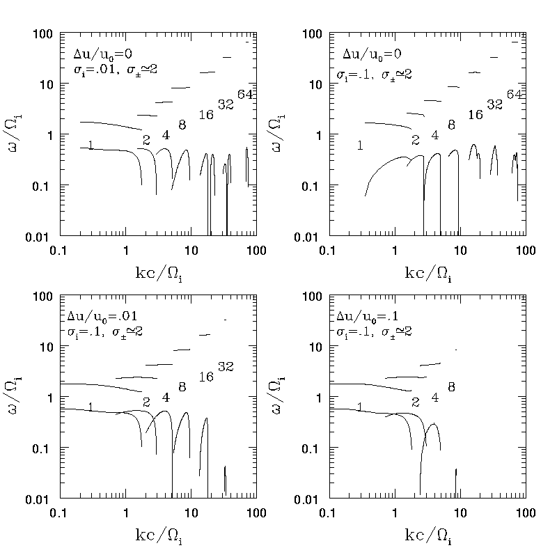
Figure 13: The dispersion relation for waves produced by the ion cyclotron instability. A mass ratio of $2000$ between the ions and the pairs is used, and the energy balance between the different components corresponds to $\sigma_{i}=0.1$ and $\sigma_{-}=2\simeq\sigma_{+}$. Upper left panel: the dispersion equation is solved in the approximation that the ions are completely cold and that mode coupling is negligible ($\varepsilon_{xy}=0$). Upper right panel: ions treated as cold but mode coupling included. Lower left panel: a thermal spread of the ions corresponding to $\Delta u/u_{0}=0.01$ (see text) is assumed. Lower right panel: a thermal spread of the ions corresponding to $\Delta u/u_{0}=0.1$ (see text) is assumed. While in the upper panels both the electromagnetic and magnetosonic wave branches have non-negligible maximum growth-rates, only magnetosonic waves are found to grow in the presence of a finite spread in the temperature of the ions.

In general, solutions of the dispersion relation are found numerically and in Fig. 13 we plot the results in a few cases relevant for the present study. In all plots we consider a plasma with $m_{i}/m_{\pm}=2000$ and with a baryon fraction $N_{i}/N_{-}=0.01$. The two upper panels refer to the case when the ions can be treated as completely cold (analogous to Hoshino & Arons (1991)). In the upper left panel the pair plasma is approximated as neutral and the coupling between the longitudinal and transverse components of the extraordinary mode is neglected $\varepsilon_{xy}=0$. In the upper right panel roots of the complete dispersion equation are shown.

When the coupling is neglected, at high harmonic numbers, the dispersion relation shows two separate unstable branches, corresponding to electromagnetic ($\omega\approx kc$) and magnetosonic waves ($\omega\approx kc\sqrt{(1/2+\sigma_{\pm})/(1+\sigma_{\pm})}$). The growth-rate of magnetosonic waves is more or less constant with increasing $n$ while the growth of electromagnetic waves is soon depressed at high harmonics. The main effect of the coupling is to further depress the growth of electromagnetic waves, whereas the growth-rate of magnetosonic waves stays about the same.

In the lower panels of Fig.13, we show the solution of the dispersion equation in cases when the ion component is not treated as perfectly cold at the onset of the instability. The plasma composition is the same as above but now a thermal spread of the ion distribution is included, with the distribution function in Eq.A1 replaced by:

$$f_{i}(u_{\perp},u_{\parallel})={\delta(u_{\parallel})\over 2\pi}\ {\exp[-(u_{\perp}-u_{0})^{2}/\Delta u^{2}]\over\sqrt{\pi}\ \Delta u\ u_{0}}\ .$$ (A8)

The effect of the thermal dispersion of the momenta depends on the effective Mach number $M_{s}\equiv u_{0i}/\Delta u$; we use this terminology, anticipating the occurrence of the ion cyclotron instability in the magnetosonic shock structures studied in §2, where $u_{0i}$ becomes the upstream 4-velocity and $\Delta u$ the upstream dispersion in the ion 4-velocity. We assume $M_{s}=0.01$ in the left panel, while the case $M_{s}=0.1$ is on the right. It is apparent that the growth of the waves is suppressed at high harmonic numbers, with the suppression affecting increasingly low harmonics the larger the distribution in perpendicular momentum space.

References

- Alsop & Arons (1988) Alsop D. & Arons J., 1988, Phys. Fluids, 31, 839
- Balucińnska-Church et al. (2005) Balucińnska-Church M., Ostrowski M., Stawarz Ł., & Church M.J., 2005, MNRAS, 357, L6
- Birdsall & Langdon (1991) Birdsall C.K. & Langdon A.B., 1991, “Plasma Physics Via Computer Simulation” (Adam Hilger, Bristol)
- Dawson (1995) Dawson J.M. 1995, Phys. Plasmas, 2, 2189
- Frederiksen et al. (2004) Frederiksen J.T. et al., 2004, Ap.J., 608, L13
- Gaensler et al. (2005) Gaensler B.M. et al., 2005, Nature, 434, 1104
- Gallant et al. (1992) Gallant Y..A. et al., 1992, ApJ, 391, 73
- Gotthelf (2003) Gotthelf, E.V., 2003, Ap.J., 591, 361
- Heavens & Meisenheimer (1987) Heavens A.F. & Meisenheimer K., 1987, MNRAS, 225, 335
- Hededahl et al. (2004) Hededahl C.B. et al., 2004, Ap.J., 617, L107
- Hededahl & Nishikawa (2005) Hededahl C.B. & Nishikawa K.I., 2005, 623, L89
- Hoshino & Arons (1991) Hoshino M. & Arons J., 1991, Phys. Fluids B, 3, 818
- Hoshino et al. (1992) Hoshino M. et al., 1992, ApJ, 390, 454
- Jaroschek (2005) Jaroschek C.H. et al., 2005, Ap.J., 618, 822
- Kaspi et al. (2004) Kaspi V., Roberts M.S.E., Harding A.K., 2004, to appear in ”Compact Stellar X-ray Sources”, eds. W.H.G. Lewin and M. van der Klis. (astro-ph/0402136)
- Kennel & Coroniti (1984) Kennel C.F. & Coroniti F.V., 1984a, ApJ, 283, 694
- Krall & Trivelpiece (1973) Krall N.A. & Trivelpiece A.W., “Principles of Plasma Physics” (McGraw-Hill, NY, 1973)
- Langdon et al. (1988) Langdon A.B. & Arons, J. & Max, C.E., 1988, Phys. Rev. Lett., 61, 779
- Lyubarsky & Eichler (2006) Lyubarsky Y. & Eichler D., 2006, Ap.J. preprint doi:10.1086/“505523” (astro-ph/0512579)
- Marscher & Gear (1985) Marscher A.P. & Gear W.K., 1985, Ap.J., 298, 114
- Milosavljevic & Nakar (2006) Milosavljevic M. & Nakar E., 2006, Ap.J., 641, 978
- Piran (2004) Piran T., 2004, Rev. Mod. Phys., 76, 1143
- Silva et al. (2003) Silva L.O. et al., 2003, Ap.J. 596, L121
- Slane (2005) Slane P., 2005, to appear in the NATO-ASI proceedings ”The Electromagnetic Spectrum of Neutron Stars”, eds. A. Baykal, S.K. Yerli, M. Gilfanov, S. Grebenev (astro-ph/0505500)
- Türler et al. (2000) Türler M., Courvoisier T. J.-L., & Paltani S., 2000, A.&A., 361, 850
- Türler et al. (2004) Türler M., Courvoisier T. J.-L., Chaty S., & Fuchs Y., 2004, A.&A., 415, L35
- Verbonocoeur, Langdon & Gladd (1995) Verbonocoeur J.P., Langdon A.B. & Gladd N.T., 1995, Computer Physics Communications, 87, 199
- Wilson, Young & Shopbell (2000) Wilson A.S., Young A.J. & Shopbell P.L., 2000, Ap.J. 544, L27
- Yoon and Davidson (1987) Yoon, P.H., and Davidson, R., 1987, Phys. Rev. A, 35, 2718