astro-ph/0608562

CERN–PH–TH/2006-168, UMN–TH–2516/06, FTPI–MINN–06/29

Bound-State Effects on Light-Element Abundances in Gravitino Dark Matter Scenarios

Richard H. Cyburt¹, John Ellis², Brian D. Fields³,

Keith A. Olive⁴, and Vassilis C. Spanos^{4 1}TRIUMF, Vancouver, BC V6T 2A3 Canada
²TH Division, PH Department, CERN, 1211 Geneva 23, Switzerland
³Departments of Astronomy and of Physics, University of Illinois, Urbana, IL 61801, USA
⁴William I. Fine Theoretical Physics Institute,
University of Minnesota, Minneapolis, MN 55455, USA
Abstract

If the gravitino is the lightest supersymmetric particle and the long-lived next-to-lightest sparticle (NSP) is the stau, the charged partner of the tau lepton, it may be metastable and form bound states with several nuclei. These bound states may affect the cosmological abundances of ⁶Li and ⁷Li by enhancing nuclear rates that would otherwise be strongly suppressed. We consider the effects of these enhanced rates on the final abundances produced in Big-Bang nucleosynthesis (BBN), including injections of both electromagnetic and hadronic energy during and after BBN. We calculate the dominant two- and three-body decays of both neutralino and stau NSPs, and model the electromagnetic and hadronic decay products using the PYTHIA event generator and a cascade equation. Generically, the introduction of bound states drives light element abundances further from their observed values; however, for small regions of parameter space bound state effects can bring lithium abundances in particular in better accord with observations. We show that in regions where the stau is the NSP with a lifetime longer than $10^{3}-10^{4}$ s, the abundances of ⁶Li and ⁷Li are far in excess of those allowed by observations. For shorter lifetimes of order $1000$ s, we comment on the possibility in minimal supersymmetric and supergravity models that stau decays could reduce the ⁷Li abundance from standard BBN values while at the same time enhancing the ⁶Li abundance.

CERN–PH–TH/2006-168

August 2006

1 Introduction

The abundances of the light nuclei produced by primordial Big-Bang nucleosynthesis (BBN) provide some of the most stringent constraints on the decays of unstable massive particles during the early Universe [1, 2, 3, 4, 5, 6, 7, 8, 9]. This is because the astrophysical determinations of the abundances of deuterium (D) and ⁴He agree well with those predicted by homogeneous BBN calculations, and also the baryon-to-photon ratio $\eta\equiv n_{b}/n_{\gamma}\propto\Omega_{b}h^{2}$ needed for the success of these calculations [10, 11] agrees very well with that inferred [12] from observations of the power spectrum of fluctuations in the cosmic microwave background (CMB). The value of $\eta=(6.11\pm 0.25)\times 10^{-10}$ that they indicate [13] is now quite precise, reducing one of the principal uncertainties in the previous BBN calculations.

However, it is still difficult to reconcile the BBN predictions for the lithium isotope abundances with observational indications on the primordial abundances. The discovery of the “Spite” plateau [14], which demonstrates a near-independence of the ⁷Li abundance from the metallicity in Population-II stars, suggests a primordial abundance in the range ${\rm\mbox{${}^{7}${\rm Li}}/H}\sim(1-2)\times 10^{-10}$  [15], whereas standard BBN with the CMB value of $\eta$ would predict ${\rm\mbox{${}^{7}${\rm Li}}/H}\sim 4\times 10^{-10}$ [10, 11]. In the case of ⁶Li, the data [16] lie a factor $\sim 1000$ above the BBN predictions [17], and fail to exhibit the dependence on metallicity expected in models based on nucleosynthesis by Galactic cosmic rays [18]. On the other hand, the ⁶Li abundance may be explained by pre-Galactic Population-III stars, without additional over-production of ⁷Li [19].

The concordance between BBN predictions and the observed abundances of D and ⁴He is relatively fragile and could have been upset by decays of massive unstable particles. Electromagnetic and hadronic showers produced in decays occurring during or shortly after BBN induce new reactions which may either create or destroy light nuclides. Concrete examples of unstable but long-lived particles are found in supersymmetric theories. In particular, models based on the constrained version of the minimal $R$-parity conserving supersymmetric standard model (CMSSM) with a gravitino as the lightest supersymmetric particle (LSP) have been considered in this context [20, 21, 22, 23, 24, 25]. In these models with a gravitino LSP, the next-to-lightest supersymmetric particle (NSP) may be either the lightest neutralino $\chi$ or the lighter stau ${\tilde{\tau}_{1}}$, and the decay lifetime of the NSP can range from seconds to years depending on the specific model and gravitino mass. Our previous results concentrated on relatively long lifetimes ($\tau>10^{4}$ s), and the effects of the electromagnetic showers on the light-element abundances [4, 21, 22, 23].

The effects of hadronic injections due to late decays of the NSP during BBN have also been studied extensively by other authors [3, 6, 7, 26, 27, 28]. In particular, it has been shown for relatively short lifetimes of order $10^{3}$ s that decays may simultaneously increase the ⁶Li abundance and decrease the ⁷Li abundance [26, 27]. On the other hand, it has been shown [23] that purely electromagnetic showers cannot reduce the ⁷Li abundance sufficiently without also overproducing D relative to ³He [29]. In [20] the authors have calculated the principal three-body decays of a stau NSP and, using the results of the analysis [6] have explored regions where the ⁷Li puzzle can be solved in an unconstrained supersymmetric model. The authors of [6] used the PYTHIA [30] model for $e^{+}e^{-}$ annihilation to hadrons in order to simulate the hadronic decays of the unstable particle. An analogous simulation was used in [24], both to locate regions in the parameter space of the CMSSM which are compatible with the BBN constraints, and to solve the lithium problem [25].

It has recently been pointed out that, if it has electric charge, the NSP forms bound states with several nuclei [31]. Due to the large NSP mass ($m_{\rm nsp}\gg m_{\rm nucleon}$), the Bohr radii of these bound states $\sim\alpha^{-1}m_{\rm nucleon}^{-1}\sim 1\ {\rm fm}$ are of order the nuclear size. Consequently, nuclear reactions with nuclei in bound states are catalyzed, due to partial screening of the Coulomb barrier, and due to the opening of virtual photon channels in radiative capture reactions. Ref. [31] used analytic approximations to argue that the $d(\alpha,\gamma)\mbox{${}^{6}${\rm Li}}$ reaction is enhanced by an enormous factor $\sim 10^{6}$, leading to ⁶Li production far beyond tolerable levels over large regions of parameter space. Other effects of bound states were considered in [32, 33].

Here, we present results from a new BBN code that includes the nuclear reactions induced by hadronic and electromagnetic showers generated by late gravitational decays of the NSP, together with the familiar network of nuclear reactions used to calculate the primordial abundances of the light elements Deuterium (D), ³He, ⁴He and ⁷Li. In addition, we include the effects of the bound states when the decaying particle is charged. As claimed in [31], these bound states lead to large enhancements in otherwise heavily suppressed rates. We calculate the abundances of the various bound states and include both the Coulomb enhancement as well as virtual photon effects in radiative capture reactions.

We use as frameworks for this study both the CMSSM and mSUGRA models [22], where the NSP could be either the lighter stau or the lightest neutralino. We have calculated the dominant two- and three-body gravitational decays of these sparticles and use the PYTHIA Monte Carlo event generator and a cascade equation to model the resulting electromagnetic (EM) and hadronic (HD) spectra for each point of the parameter space of the supersymmetric model. The resulting accurate determinations of the abundances of the light elements, as altered by these late injections and the bound-state effects, enable us to delineate regions of the parameter space of the supersymmetric models which are compatible with the BBN constraints. In addition, we look for regions where the ⁶Li and ⁷Li puzzles can be solved in the context of these supersymmetric models. We find that for lifetimes $\tau<10^{3}-10^{4}$ s, the enhanced rates of ⁶Li and ⁷Li production, exclude gravitino dark matter (GDM) with a stau NSP. At smaller lifetimes, we see that it is the ⁷Li destruction rates which are enhanced, facilitating a solution to the Li problems.

2 Electromagnetic and Hadronic NSP Decays

The CMSSM is determined by four real parameters, namely the soft supersymmetry-breaking scalar mass $m_{0}$, the gaugino mass $m_{1/2}$, the trilinear coupling $A_{0}$ (each taken to be universal at the Grand Unification scale), the ratio of Higgs vevs $\tan\beta$, and the sign of the $\mu$ parameter. Here, for simplicity, we restrict our attention to $A_{0}=0$ and $\mu>0$. The mass of the gravitino is also a free parameter in the CMSSM, and if is chosen to be less than $\min(m_{\chi},m_{\tilde{\tau}})$ the resultant model has GDM. In mSUGRA models [22], $\tan\beta$ is no longer a free parameter, nor is the gravitino mass which is now equal to $m_{0}$ at the Grand Unification scale. GDM is a inevitable consequence in mSUGRA models when $m_{0}$ is relatively small. In this case, the NSP is typically the stau, but it may also be the neutralino if $A_{0}/m_{0}\mathrel{\raise 1.29167pt\hbox{$<$\kern-7.5pt\lower 4.30554pt\hbox{$\sim$}}}1.7$. The abundances of light elements provide some of the most important constraints on this gravitino LSP scenario [20, 21, 22, 23, 24, 25]. They also impose important constraints on the neutralino LSP scenario, since a gravitino NSP would also decay slowly. Here, however, we restrict our attention to GDM scenarios with either a stau or neutralino NSP.

In order to estimate the lifetime of the NSP, as well as the various branching ratios and the resulting EM and HD spectra, one must calculate the partial widths of the dominant relevant decay channels of the NSP . The decay products that yield EM energy obviously include directly-produced photons, and also indirectly-produced photons, charged leptons (electrons and muons) which are produced via the secondary decays of gauge and Higgs bosons, as well as neutral pions ($\pi^{0}$). Hadrons (nucleons and mesons such as the $K_{L}^{0}$, $K^{\pm}$ and $\pi^{\pm}$) are usually produced through the secondary decays of gauge and Higgs bosons, as well (for the mesons) as via the decays of the heavy $\tau$ lepton. It is important to note that mesons decay before interacting with the hadronic background [3, 20]. Hence they are irrelevant to the BBN processes and to our analysis, except via their decays into photons and charged leptons. Therefore, the HD injections on which we focus our attention are those that produce nucleons, namely the decays via gauge and Higgs bosons and quark-antiquark pairs.

For the neutralino NSP $\chi$, we include the two-body decay channels $\chi\to\widetilde{G}\,H_{i}$ and $\chi\to\widetilde{G}\,V$, where $H_{i}=h,H,A$ and $V=\gamma,Z$. These are the dominant gravitational decays of $\chi$, whose analytical expressions have been presented in [21]. In addition, we include here the dominant three-body decays $\chi\to\widetilde{G}\,\gamma^{*}\to\widetilde{G}\,q\overline{q}$, $\chi\to\widetilde{G}\,\gamma^{*}\to\widetilde{G}\,W^{+}W^{-}$, $\chi\to\widetilde{G}\,W^{+}W^{-}$ and the corresponding interference terms. In general, the two-body channel $\chi\to\widetilde{G}\,\gamma$ dominates the $\chi$ NSP decays and yields the bulk of the injected EM energy. When the $\chi$ is heavy enough to produce a real $Z$ boson, the next most important channel is $\chi\to\widetilde{G}\,Z$, which is also the dominant channel for producing HD injections in this case. The Higgs boson channels are smaller by a few orders of magnitude, and those to heavy Higgs bosons ($H,A$) in particular become kinematically accessible only for heavy $\chi$ in the large-$m_{1/2}$ region. Turning to the three-body channels, the decay through the virtual photon to a $q\overline{q}$ pair can become comparable to the subdominant channel $\chi\to\widetilde{G}\,Z$, injecting nucleons even in the kinematical region $m_{\chi}<m_{3/2}+M_{Z}$, where direct on-shell $Z$-boson production is not possible . Finally, we note that the three-body decays to $W^{+}W^{-}$ pairs and a gravitino are usually at least five orders of magnitude smaller.

For general orientation, we present in Fig. 1 contours (in seconds) for the supersymmetric models discussed later and presented in Figs. 2 and 3. We display the $m_{1/2},m_{0}$ planes for variants of the CMSSM with different gravitino masses for $\tan\beta=10,A_{0}=0$ (panels a and b), and $\tan\beta=57,A_{0}=0$ (panel c). Panel d displays an analogous plane for a mSUGRA model with $A_{0}/m_{0}=3-\sqrt{3}$ at the GUT scale, in which $\tan\beta$ is determined at each point by the electroweak vacuum conditions. In addition to the NSP lifetime contours (labelled by the lifetime in seconds), we show the boundaries between regions with neutralino and stau NSPs (dotted red lines) and the upper limit on the gravitino mass density (solid brown lines). These curves are also found in Figs. 2 and 3.

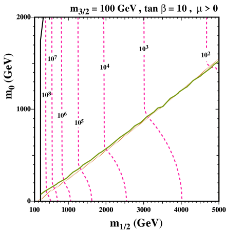
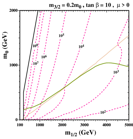
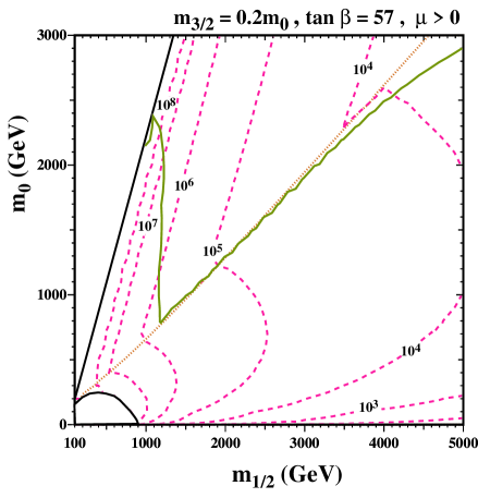
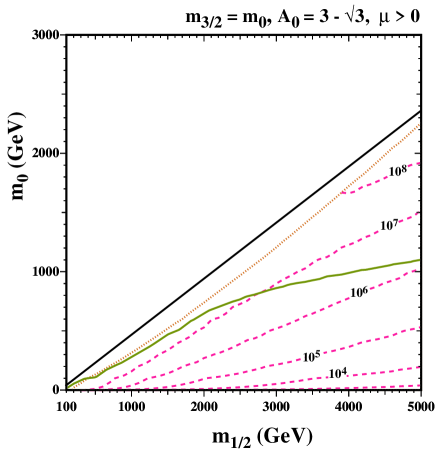
Figure 1: The NSP lifetime contours (in seconds) for the supersymmetric models discussed in Figs. 2 and 3.

Having calculated the partial decay widths and branching ratios, we employ the PYTHIA event generator [30] to model both the EM and the HD decays of the direct products of the $\chi$ decays. We first generate a sufficient number of spectra for the secondary decays of the gauge and Higgs bosons and the quark pairs. Then, we perform fits to obtain the relation between the energy of the decaying particle and the quantity that characterizes the hadronic spectrum, namely $dN_{h}/dE_{h}$, the number of produced nucleons as a function of the nucleon energy. These spectra and the fraction of the energy of the decaying particle that is injected as EM energy are then used to calculate the light-element abundances.

An analogous procedure is followed for the $\tilde{\tau}$ NSP case. As the lighter stau is predominantly right-handed, its interactions with $W$ bosons are very weak (suppressed by powers of $m_{\tau}$) and can be ignored. The decay rate for the dominant two-body decay channel, namely $\tilde{\tau}\to\widetilde{G}\,\tau$, has been given in [21]. However, this decay channel does not yield any nucleons. Therefore, one must calculate some three-body decays of the $\tilde{\tau}$ to obtain any protons or neutrons. The most relevant channels are $\tilde{\tau}\to\widetilde{G}\,\tau^{*}\to\widetilde{G}\,Z\,\tau$, $\tilde{\tau}\to Z\,\tilde{\tau}^{*}\to\widetilde{G}\,Z\,\tau$, $\tilde{\tau}\to\tau\chi^{*}\to\widetilde{G}\,Z\,\tau$ and $\tilde{\tau}\to\widetilde{G}\,Z\,\tau$ [20]. We calculate these partial widths, and then use PYTHIA to obtain the hadronic spectra and the EM energy injected by the secondary $Z$-boson and $\tau$-lepton decays. As in the case of the $\chi$ NSP, this information is then used for the BBN calculation.

We stress that this procedure is repeated separately for each point in the supersymmetric parameter space sampled. That is, given a set of parameters $m_{0},m_{1/2},A_{0},\tan\beta$, sgn$(\mu)$, and $m_{3/2}$, once the sparticle spectrum is determined, all of the relevant branching fractions are computed, and the hadronic spectra and the injected EM energy determined case by case. For this reason, we do not use a global parameter such as the hadronic branching fraction, $B_{h}$, often used in the literature. In our analysis, $B_{h}$ is computed and differs at each point in the parameter space.

3 Electromagnetic and Hadronic Showers During Primordial Nucleosynthesis

The dominant effect of hadronic decays of the NSP during BBN is the addition of new interactions between hadronic shower particles and background nuclides . These alter the evolution and final values of the light-element abundances, as follows. For each background species $i$, let the rate of interactions of decay hadrons per background particle be $\Gamma_{i}$. Then the $i$ abundance per background baryon, $Y_{i}=n_{i}/n_{B}$, changes according to

$$\partial_{t}Y_{i}=\left(\partial_{t}Y_{i}\right)_{\rm SBBN}+\left(\partial_{t}Y_{i}\right)_{\rm HAD}+\left(\partial_{t}Y_{i}\right)_{\rm EM},$$ (1)

where $\dot{Y}_{\rm SBBN}$ gives the rate of change of the $i$ abundance in standard BBN. We have also included in (1) the effects of electromagnetic interactions due to NSP decays, either from the decays directly to photons or leptons, or through electromagnetic secondaries in the hadronic showers. These are treated as in [4], but are not dominant when hadronic branchings are significant. All we need to know is the total EM energy released per decay in any given channel, which may become more complicated in the three-body case, but can easily be calculated.

Including hadronic decays in BBN thus amounts to an evaluation of the interaction rates

$$\left(\partial_{t}Y_{i}\right)_{\rm HAD}=-\Gamma_{\rm i\rightarrow{\rm inel}}Y_{i}+\sum_{hb}\Gamma_{hb\rightarrow i}Y_{b}.$$ (2)

The first term accounts for $i$ destruction by hadro-dissociation, where $\Gamma_{\rm i\rightarrow{\rm inel}}$ is the total rate (for a given species $i$) of all inelastic interactions of shower particles with $i$. The second term accounts for production via the hadro-dissociation of heavier background species, e.g., $p_{\rm shower}\alpha_{\rm bg}\rightarrow d$. The sum runs over shower species $h$ and background targets $b$. In the case of the lithium isotopes, production also occurs via the interactions of energetic (i.e., nonthermal) mass-3 dissociation products with background ⁴He, e.g., $\mbox{${}^{3}${\rm He}}\alpha\rightarrow\mbox{${}^{6,7}${\rm Li}}+\cdots$.

Consider a nonthermal hadronic projectile species $h$, with energy spectrum $N_{h}(\epsilon,t)=dN_{h}/dVd\epsilon$ and total number density $n_{h}=\int N_{h}d\epsilon$. The rate for $i$ production due to $hb\rightarrow i$ is

$$\Gamma_{hb\rightarrow i}=\int N_{h}(\epsilon,t)\sigma_{hb\rightarrow i}(\epsilon)d\epsilon.$$ (3)

The rates $\Gamma_{i}$ thus depend on the decay particle, on the background abundances, and most importantly from the point of view of implementation, on the shower development and evolution of $N_{h,\epsilon}$ in the background environment.

We wish to follow the evolution of $N_{h}$ over the multiple shower generations produced by the initial hadronic NSP decay products. In the context of BBN, this problem of shower development has been approached via direct computation of the multiple generations of shower particles [3, 2, 26]. In this approach, the final particle spectrum is obtained by iterating an initial decay spectrum, accounting for both the energy losses and the energy distributions of collision products.

We introduce here an equivalent alternative approach, based on a cascade equation, emulating the well-studied treatment of hadronic shower development due to cosmic-ray interactions in the atmosphere. The spectrum of $h$ evolves according to

$$\partial_{t}N_{h}(\epsilon)=J_{h}(\epsilon)-\Lambda_{h}(\epsilon)N_{h}(\epsilon)-\partial_{\epsilon}\left[b_{h}(\epsilon)N_{h}(\epsilon)\right],$$ (4)

where $J_{h}$ is the sum of all source terms, $\Lambda_{h}$ is the sum of all sink terms, and $b_{h}$ is the energy-loss rate of particle-conserving processes. The energy-loss term is assumed to be the dominant process of energy transfer, in which case tertiary processes are limited to down-scattering. The sink term has two contributions, due to elastic and inelastic scattering; the source term has three contributions, due to direct injection, elastic down-scattering and inelastic down-scattering.

Each nonthermal species $i$ evolves according to a cascade equation of the form (4), and together these constitute a coupled set of equations. Because the source term includes the elastic term with $N_{i}$ inside the integral, these equations are of integro-differential form. The integration is therefore not immediate. Previous work on hadronic decays has adopted a Monte Carlo approach to the solution; our method is to solve the differential equation.

We note that because this is an integral equation, we can adopt an iterative approach to the solution. To make our initial guess, we ignore the downscattering and solve for $N_{h}$ with decays being the only source. The solution can then be written in terms of the following quadrature

$$N_{h}^{(i)}(\epsilon,t)=\frac{1}{b(\epsilon)}\int_{\epsilon}^{\infty}d\epsilon^{\prime}\ J_{h}^{(i)}(\epsilon^{\prime},t)\ e^{-R(\epsilon^{\prime},t)},$$ (5)

where our initial guess takes $J_{h}^{(0)}=q_{X}(\epsilon)$ only. Here the exponential “optical depth” factor

$$R(\epsilon^{\prime},t)=\int_{\epsilon}^{\epsilon^{\prime}}d\epsilon^{\prime\prime}\ \frac{\Gamma(\epsilon^{\prime\prime},t)}{b(\epsilon^{\prime\prime})}$$ (6)

is a measure of the average number of inelastic interactions over the time taken to lose energy electromagnetically from $\epsilon^{\prime}$ to $\epsilon$.

The full cascades can then be treated iteratively, correcting the approximation to include the redistribution and production of nucleons in scattering events. We do this by using the previous solution $N_{h}^{(i)}$ to update the source term $J_{h}^{(i+1)}$ by including the downscattering terms. These distributions converge after a few iterations. We then insert them into (2) and solve for the hadro-dissociation rate. This iterative procedure is similar to what previous studies have done. However, rather than including the exponent in the integral, they treat the exponential $R$ term as a delta function, evaluated at $\epsilon_{*}$ ($R(\epsilon_{*},\epsilon,t)=1$).

Full details of our method will be given in [9].

4 Bound-State Effects

It has recently been pointed out [31] that the presence of a charged particle, such as the stau, during BBN can alter the light-element abundances in a significant way due to the formation negatively-charged staus of bound states (BS) with charged nuclei. The binding energies of these states are $\alpha^{2}Z_{i}^{2}m_{i}/2\approx 30Z_{i}^{2}A_{i}\ {\rm keV}$, and the Bohr radii $\sim(\alpha Z_{i}m_{i})\sim 1\ Z_{i}^{-1}A_{i}^{-1}\ {\rm fm}$. For species such as ⁴He, ⁷Li and ⁷Be, these energy and length scales are close to those of nuclear interactions, and it thus turns out that bound state formation results in catalysis of nuclear rates via two mechanisms.

One immediate consequence of the bound states is a reduction of the Coulomb barrier for nuclear reactions, due to partial screening by the stau. Since Coulomb repulsion dominates the charged-particle rates, all such rates are enhanced. Specifically, for the case of an initial state $A_{1}+A_{2}$, Coulomb effects lead to a exponential suppression via a penetration factor which scales as $Z_{1}^{2/3}Z_{2}^{2/3}A^{1/3}$, with $A=A_{1}A_{2}/(A_{1}+A_{2})$. Introduction of a bound state $(\tilde{\tau},A_{2})$ decreases the target charge to $Z_{2}-1$ and the system’s reduced mass number to $A=A_{1}$; both effects lower the Coulomb suppression. We include these effects for all reactions with bound states.

Table 1: Bound-state virtual photon enhancements to radiative capture cross sections for various reactions. The third (fourth) column is the threshold energy for the standard (catalyzed) BBN. The last column is the virtual photon enhancement factor of the catalyzed cross section relative to standard BBN.

	EM	$A(B,\gamma)$	$[X^{-}A](B,C)X^{-}$	Enhancement
Reaction	Transition	$Q_{\rm SBBN}$ (MeV)	$Q_{\rm CBBN}$ (MeV)	$\sigma_{\rm CBBN}/\sigma_{\rm SBBN}$
$d(\alpha,\gamma$)6Li	E2	1.474	1.124	7.0$\times 10^{7}$
3H($\alpha,\gamma$)7Li	E1	2.467	2.117	1.0$\times 10^{5}$
3He($\alpha,\gamma$)7Be	E1	1.587	1.237	2.9$\times 10^{5}$
6Li($p,\gamma$)7Be	E1	5.606	4.716	2.9$\times 10^{4}$
7Li($p,\gamma$)8Be	E1	17.255	16.325	2.6$\times 10^{3}$
7Be($p,\gamma$)8B	E1	0.137	-1.323	N/A

An additional effect enhances radiative capture channels $A_{2}(A_{1},\gamma)X$ by introducing photonless final states in which the stau carries off the reaction energy transmitted via virtual photon processes. In particular, the $\mbox{${}^{4}${\rm He}}(d,\gamma)\mbox{${}^{6}${\rm Li}}$ reaction, which is suppressed in standard BBN, is enhanced by many orders of magnitude by the presence of the bound states, as described in [31]. Large enhancements of this type affect other radiative capture reactions, notably mass-7 production reactions such as $\mbox{${}^{3}${\rm He}}(\alpha,\gamma)\mbox{${}^{7}${\rm Be}}$ and destruction reactions such as $\mbox{${}^{7}${\rm Li}}(\alpha,\gamma)\mbox{${}^{11}${\rm B}}$. We have included these as well: the corresponding enhancement factors appear in Table 1.

Bound-state formation and reaction catalysis occurs late in BBN. The binding energy $E_{\textrm{bin}}$ for the [$\tilde{\tau},\mbox{${}^{4}${\rm He}}$] bound states is 311 keV, for [$\tilde{\tau},\mbox{${}^{7}${\rm Li}}$] 952 keV, and for the [$\tilde{\tau},\mbox{${}^{7}${\rm Be}}$] 1490 keV. The latter are quite high, of order nuclear binding energies, and indeed the large ⁷Be binding plays an important role in forbidding ⁷Be destruction channels that otherwise would be energetically allowed. The capture processes that form these bound states typically become effective for temperatures $T_{c}\approx E_{\textrm{bin}}/30$; this means that ⁷Be states form prior to ⁷Li states, with ⁴He states forming last. At these low temperatures one can ignore the standard BBN fusion processes that involve these elements.

To account for bound state effects, an accurate calculation of their abundance is necessary. To do this we solve numerically the Boltzmann equations (13) and (14) from [32], that control these abundances. If $X$ denotes the light element, and ignoring the fusion contribution as described before, the system of the two differential equations for the light-element and bound state abundances can be cast into the form

$$\dot{Y}_{X} = \frac{\left\langle\sigma_{c}v\right\rangle}{H\,T}\,(Y_{X}\,n_{\tilde{\tau}}-Y_{BS}\,n^{\prime}_{\gamma})$$

$$\dot{Y}_{BS} = -\dot{Y}_{X}\,,$$ (7)

where $Y_{BS,X}=n_{BS,X}/s$ and $n_{\tilde{\tau}}$ is the stau number density. The thermally-averaged capture cross section $\left\langle\sigma_{c}v\right\rangle$ and the photon density $n^{\prime}_{\gamma}$ for $E>E_{\textrm{bin}}$, are given in Eqs (9) and (15) in [32], respectively. $H$ is the Hubble expansion and dot denotes derivatives with respect to the temperature. As initial condition, we assume that the bound state abundance is negligible for a temperature of a few times $T_{c}$. In our numerical analysis we solve the system (7) for $X=\mbox{${}^{4}${\rm He}},\mbox{${}^{7}${\rm Li}},\mbox{${}^{7}${\rm Be}}$ to obtain the corresponding $Y_{BS}$ at temperatures below $T_{c}$. We assume that the bound state is destroyed in the reaction. That is, we do not include additional bound-state effects on the final-state nuclei such as ⁶Li.

As we see in the following section, bound state effects indeed greatly enhance ⁶Li production as found in the analysis of $d(\alpha,\gamma)\mbox{${}^{6}${\rm Li}}$ by [31]. Our systematic inclusion of bound state effects finds that ⁷Li is also significantly altered. The most important rates are for radiative capture reactions, which enjoy large boosts due to virtual photon effects. In particular, bound state ⁷Li production is dominated by the $\mbox{${}^{3}${\rm H}}(\alpha,\gamma)\mbox{${}^{7}${\rm Li}}$ and $\mbox{${}^{3}${\rm He}}(\alpha,\gamma)\mbox{${}^{7}${\rm Be}}$ rates. Destruction is dominated by the channel with the lowest Coulomb barrier, namely $\mbox{${}^{7}${\rm Li}}(p,\gamma)2\mbox{${}^{4}${\rm He}}$. Note that ⁷Be destruction channels are less important, since mass-7 is largely in ⁷Li at $T\mathrel{\raise 1.29167pt\hbox{$>$\kern-7.5pt\lower 4.30554pt\hbox{$\sim$}}}60$ keV, and because the high binding energy of [$\tilde{\tau},\mbox{${}^{7}${\rm Be}}$] makes $[\tilde{\tau},\mbox{${}^{7}${\rm Be}}]+p\rightarrow\mbox{${}^{8}${\rm B}}+\tilde{\tau}$ energetically forbidden with $Q=-1.3$ MeV (see Table 1).

Interestingly, the bound state perturbations lead to net ⁷Li production in some parts of the parameter space of the models we study, and net destruction in others. Net production occurs when the stau is sufficiently long-lived ($\tau_{\tilde{\tau}}\mathrel{\raise 1.29167pt\hbox{$>$\kern-7.5pt\lower 4.30554pt\hbox{$\sim$}}}10^{4}$ sec) that ⁴He bound states are abundant enough to drive bound state enhanced production stronger than bound state enhanced ⁷Li destruction. On the other hand, within a window of slightly shorter lifetimes, staus persist long enough to form ⁷Li bound states, but then decay before forming ⁴He bound states. This leads to net ⁷Li destruction. Thus we see that ⁷Li is quite sensitive to the $\tilde{\tau}$ properties, and potentially offers a strong probe of the existence and nature of bound states.

5 Results and Discussion

As described earlier, we work in the context of the CMSSM or mSUGRA. Our primary goal is to examine the effect of bound-state interactions on the final abundances of the light elements. To this end, we display a selection of results for specific supersymmetric planes both with and without the effect of bound state interactions. All results shown fully incorporate the effects of electromagnetic and hadronic showers. A more complete selection of results as well as constraints which go beyond the MSSM will be presented in [9].

We begin with results based on CMSSM models with $A_{0}=0$, $\mu>0$ and $\tan\beta=10$. We display our results in the $(m_{1/2},m_{0})$ plane, showing explicit element abundance contours. In Fig. 2a, we show the element abundances that result when the gravitino mass is held fixed at $m_{3/2}=100$ GeV in the absence of stau bound state effects. To the left of the near-vertical solid black line at $m_{1/2}\simeq 250$ GeV, the gravitino is the not the LSP, and we do not consider this region here. Immediately to the right of this line is a red dot-dashed line. To the left of this, the Higgs mass is below the current experimental bound $114{\rm\,Ge\kern-1.25ptV}$. The diagonal red dotted line corresponds to the boundary between a neutralino and stau NSP. Above the line, the neutralino is the NSP, and below it, the NSP is the stau. Very close to this boundary, there is a diagonal brown solid line. Above this line, the relic density of gravitinos from NSP decay is too high, i.e.,

$$\frac{m_{3/2}}{m_{NSP}}\Omega_{NSP}h^{2}>0.12.$$ (8)

Thus we should restrict our attention to the area below this line. Note that we display the extensions of contours which originate below the line into the overdense region, but we do not display contours that reside solely in the upper plane.

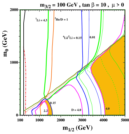
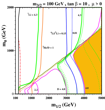
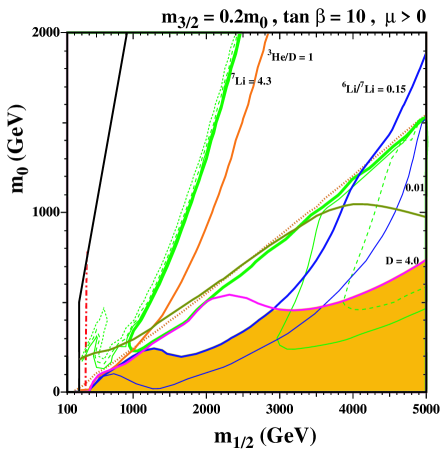
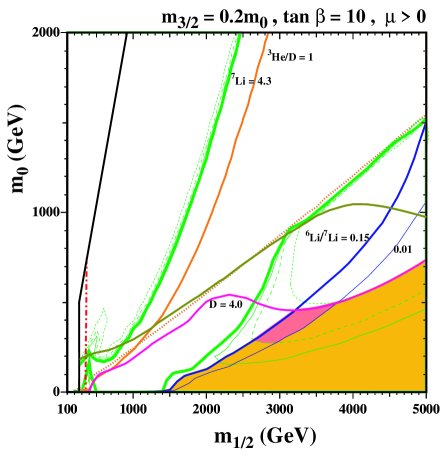
Figure 2: Some $(m_{1/2},m_{0})$ planes for $A_{0}=0$, $\mu>0$ and $\tan\beta=10$. In the upper (lower) panels we use $m_{3/2}=100$ GeV $(m_{3/2}=0.2\,m_{0})$. In the right panels the effects of the stau bound states have been included, while in those on the left we include only the effect of the NSP decays. The regions to the left of the solid black lines are not considered, since there the gravitino is not the LSP. In the orange (light) shaded regions, the differences between the calculated and observed light-element abundances are no greater than in standard BBN without late particle decays. In the pink (dark) shaded region in panel d, the abundances lie within the ranges favoured by observation, as described in the text. The significances of the other lines and contours are explained in the text.

We start with the solid orange line labelled ³He/D = 1. To the left of this curve, the ³He/D ratio is greater than 1, which is excluded [29]. For small $m_{0}$, this excludes gaugino masses less than about 1100 GeV, which is similar to the result found in [23]. To the right of this curve, the ratio of ³He to D is acceptable. The very thick green line labelled ⁷Li = 4.3 corresponds to the contour where ⁷Li/H = $4.3\times 10^{-10}$, a value very close to the standard BBN result for ⁷Li/H. It forms a ‘V’ shape, whose right edge runs along the neutralino-stau NSP border before shooting up at $m_{1/2}\sim 3900$ GeV. Below the V, the abundance of ⁷Li is smaller than the standard BBN result. However, for relatively small values of $m_{1/2}$, the ⁷Li abundance does not differ very much from this standard BBN result: it is only when $m_{1/2}\mathrel{\raise 1.29167pt\hbox{$>$\kern-7.5pt\lower 4.30554pt\hbox{$\sim$}}}3000$ GeV that ⁷Li begins to drop significantly. This is seen by the additional (unlabeled) thin green contours showing ⁷Li/H = $3\times 10^{-10}$ (solid), and $2\times 10^{-10}$ (dashed). As can be seen in Fig. 1a, the the stau lifetime drops with increasing $m_{1/2}$, and when $\tau\sim 1000$ s, at $m_{1/2}\sim 4000$ GeV, the ⁷Li abundance has been reduced to an observation-friendly value close to $2\times 10^{-10}$ as claimed in [27].

However, for this case with $m_{3/2}=100$ GeV the ⁶Li abundance is never sufficiently high to match the observed ⁶Li plateau for the same parameter values where ⁷Li is reduced. The ⁶Li/⁷Li ratio is shown by the solid blue contour labeled ⁶Li/⁷Li = 0.15. Note that there is also a small contour loop at this value at small $m_{0}$ centred around $m_{1/2}\sim 1000$ GeV. Inside the loop, the lithium isotope ratio is acceptable, which is also the case to the right of the nearly vertical contour at large $m_{1/2}$. At large $m_{1/2}$, the contour for ⁶Li/⁷Li = 0.01 is shown by the thin blue line. To the right of this contour, including the region where ⁷Li $\sim 2\times 10^{-10}$, the ⁶Li abundance is too small.

Finally, we show the contours for D/H = 2.2 and 4.0 $\times 10^{-5}$ by the solid purple contours as labeled. The D/H = 2.2 $\times 10^{-5}$ contour is a small loop within the ⁶Li/⁷Li loop. Inside this loop D/H is too small. Between the two curves labeled 4.0, the D/H ratio is high, but not necessarily excessively so.

In summary, the acceptable regions found in Fig. 2a break down into 2 areas: one between the two loops labeled 2.2 and 0.15 and to the right of the ³He/D = 1 line, where D/H is larger than 2.2 $\times 10^{-5}$ and $\mbox{${}^{6}${\rm Li}}/\mbox{${}^{7}${\rm Li}}<0.15$. However, in this region, the ⁷Li abundance is very similar to the standard BBN result, which may be considered too high. Alternatively, one could consider very large $m_{1/2}$ where once again D/H $<4.0\times 10^{-5}$. Here, ⁷Li is in fact acceptably low, but the ⁶Li abundance is far below the plateau value. As a better illustration of our results, we have shaded these two regions. The orange (lighter) shaded region is where $\mbox{${}^{3}${\rm He}}/D<1$, $\mbox{${}^{6}${\rm Li}}/\mbox{${}^{7}${\rm Li}}<0.15$, $2.2\times 10^{-5}<D/\textrm{H}<4.0\times 10^{-5}$ and $\mbox{${}^{7}${\rm Li}}/\textrm{H}<4.3\times 10^{-10}$.

Turning now to Fig. 2b, we show the analogous results when the bound-state effects are included in the calculation. The abundance contours are identical to those in Fig. 2a above the diagonal dotted line, where the NSP is a neutralino and bound states do not form. We also note that the bound state effects on D and ³He are quite minimal, so that these element abundances are very similar to those in Fig. 2a. However, comparing panels a and b, one sees dramatic bound-state effects on the lithium abundances. The loop of ⁶Li/⁷Li = 0.15 centred about $m_{1/2}=1000$ GeV has now gone due to the large abundance of ⁶Li produced by bound-state catalysis. Indeed, everywhere to the left of the solid blue line labeled 0.15 is excluded. In the stau NSP region, this means that $m_{1/2}\mathrel{\raise 1.29167pt\hbox{$>$\kern-7.5pt\lower 4.30554pt\hbox{$\sim$}}}3000-3500$ GeV. Moreover, in the stau region to the right of the ⁶Li/⁷Li = 0.15 contour, the ⁷Li abundance drops below $9\times 10^{-11}$ (as shown by the thin green dotted curve) and D/H $>4\times 10^{-5}$ for $m_{1/2}\mathrel{\raise 1.29167pt\hbox{$<$\kern-7.5pt\lower 4.30554pt\hbox{$\sim$}}}3500-4000$ GeV. Only when $m_{1/2}\mathrel{\raise 1.29167pt\hbox{$>$\kern-7.5pt\lower 4.30554pt\hbox{$\sim$}}}3500-4000$ GeV does the D/H abundance drop back to acceptable levels with good abundances for ⁷Li, but ⁶Li is now too small to account for the plateau. Thus, for a constant value of $m_{3/2}=100$ GeV, the bound-state effects force one to extremely large values of $m_{1/2}$ primarily due to the enhanced production of ⁶Li, as shown by the orange shaded region. For this value of the gravitino mass, there are no regions where both lithium abundances match their plateau values.

We do not display the results for $m_{3/2}=10$ GeV, but the bound-state effects (and the results) are less dramatic. Without the bound-state effects included, the ⁶Li abundance is generally too small, while the ⁷Li abundance is very similar to standard BBN in the stau NSP region. The gravitino relic density is a factor of 10 smaller in this case and some of the neutralino NSP region is allowable. In the neutralino NSP region, D/H is too high unless $m_{1/2}\mathrel{\raise 1.29167pt\hbox{$>$\kern-7.5pt\lower 4.30554pt\hbox{$\sim$}}}2000$ GeV. At $(m_{1/2},m_{0})\simeq(2100,1000)$, there is a region where D/H and ⁷Li are acceptably small, though ⁶Li/⁷Li is very small. The bound-state effects again set a lower limit on $m_{1/2}$ in the stau NSP region in this case. When $m_{1/2}\mathrel{\raise 1.29167pt\hbox{$>$\kern-7.5pt\lower 4.30554pt\hbox{$\sim$}}}1300$ GeV, both Li abundances drop and approach their standard BBN values. Once again, in no region are both lithium isotopes at their plateau values.

It is also interesting to consider cases in which the gravitino mass is proportional to $m_{0}$. In Fig. 2c, we fix $m_{3/2}=0.2\,m_{0}$ and neglect the bound-state effects. The choices of contours are similar to those in panels a and b. The gravitino relic density constraint now cuts out some of the stau NSP region at large $m_{1/2}$ and large $m_{0}$, but allows a small neutralino NSP region at low $m_{1/2}$. As before, we are constrained to the right of the curve labeled ³He/D = 1, though in this case the constraint is not very strong in the stau NSP region. The ⁷Li/H = $4.3\times 10^{-10}$ contour again forms a ‘V’ shape and one is restricted to lie below the ‘V’. In most of the stau NSP region, ⁷Li remains relatively high but begins to drop at large $m_{1/2}\sim 3000$ GeV as $\tau$ approaches $O(1000)$ s (see Fig. 1). The region where the ⁶Li/⁷Li ratio lies between 0.01 and 0.15 now forms a band which moves from lower left to upper right. Thus, as one can see in the orange shading, there is a large region where the lithium isotopic ratio can be made acceptable. However, if we restrict to D/H $<4.0\times 10^{-5}$, we see that this ratio is interesting only when ⁷Li is at or slightly below the standard BBN result. However, we do note that as one approaches the gravitino density limit at $(m_{1/2},m_{0})\simeq(4100,1000)$, it is possible to have ⁶Li/⁷Li $\simeq 0.06$ and ⁷Li/H $\simeq 2.3\times 10^{-10}$ at the expense of D/H $\simeq 6.2\times 10^{-10}$.

The bound-state effects when $m_{3/2}=0.2\,m_{0}$ are shown in Fig. 2d. Once again, we see that the increased production of both ⁶Li and ⁷Li excludes a portion of the stau NSP region where $m_{1/2}\mathrel{\raise 1.29167pt\hbox{$<$\kern-7.5pt\lower 4.30554pt\hbox{$\sim$}}}1500$ GeV for small $m_{0}$. The lower bound on $m_{1/2}$ increases with $m_{0}$. In this case, not only do the bound-state effects increase the ⁷Li abundance when $m_{1/2}$ is small (i.e., at relatively long stau lifetimes), but they also decrease the ⁷Li abundance when the lifetime of the stau is about 1500 s. Thus, at $(m_{1/2},m_{0})\simeq(3200,400)$, we find that ⁶Li/⁷Li $\simeq 0.04$, ⁷Li/H $\simeq 1.2\times 10^{-10}$, and D/H $\simeq 3.8\times 10^{5}$. Indeed, when $m_{1/2}$ is between 3000-4000 GeV, the bound state effects cut the ⁷Li abundance roughly in half. In the darker (pink) region (which has no analogue in the other panels), the lithium abundances match the observational plateau values, with the properties $\mbox{${}^{6}${\rm Li}}/\mbox{${}^{7}${\rm Li}}>0.01$ and $0.9\times 10^{-10}<\mbox{${}^{7}${\rm Li}}/\textrm{H}<2.0\times 10^{-10}$.

For a larger ratio of $m_{3/2}=m_{0}$, the gravitino relic density forces us to relatively low values of $m_{0}\mathrel{\raise 1.29167pt\hbox{$<$\kern-7.5pt\lower 4.30554pt\hbox{$\sim$}}}500$ GeV. As in the case described above, the viable region at low $m_{1/2}$ is excluded by the bound-state effects, and we find increased ⁷Li production due to bound states at high $m_{1/2}$. Qualitatively, this case is similar to that when $m_{3/2}=0.2\,m_{0}$, though most features are compressed to lower values of $m_{0}$.

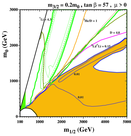
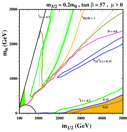
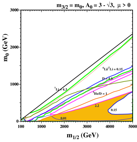
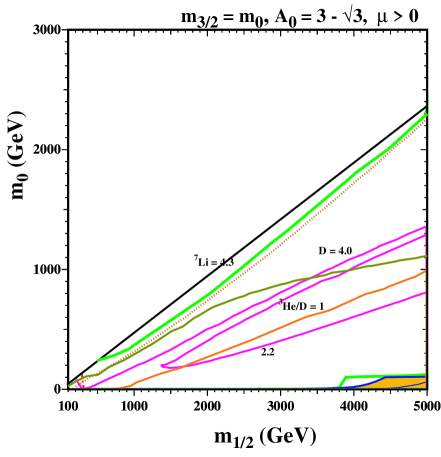
Figure 3: Some more $(m_{1/2},m_{0})$ planes for $\mu>0$. In the upper panels we use $m_{3/2}=0.2\,m_{0}$ and $\tan\beta=57$, whilst in the lower panels we assume mSUGRA with $m_{3/2}=m_{0}$ and $A_{0}/m_{0}=3-\sqrt{3}$ as in the simplest Polonyi superpotential. In the right panels the effects of the stau bound states have been included, while in those on the left we include only the effects of the NSP decays. As in Fig. 2, the region above the solid black line is excluded, since there the gravitino is not the LSP. In the orange shaded regions, the differences between the calculated and observed light-element abundances are no greater than in standard BBN without late particle decays. The meanings of the other lines and contours are explained in the text.

In Fig. 3, we show some examples of results from CMSSM models with $\tan\beta=57$, and mSUGRA models. The dominant effect of increasing $\tan\beta$ is on the neutralino and stau relic densities. At low $\tan\beta$, the relic density of the neutralino is generally high except along a narrow strip where neutralino-stau co-annihilations are important and yield a density with in the WMAP range. At large $\tan\beta$, new annihilation channels are available. Most predominant is the the s-channel annihilation of neutralinos through the heavy Higgs scalar and pseudoscalar, causing large variations in the relic density across the plane, particularly at large $m_{1/2}$ and $m_{0}$. These variations have an impact in GDM scenarios, as the abundance of decaying particles varies.

In Fig. 3a, we show the $(m_{1/2},m_{0})$ plane for $\tan\beta=57$ (which is near the maximal value for which the electroweak symmetry breaking conditions can be satisfied), and $m_{3/2}=0.2\,m_{0}$. The dark green shaded region at very low $m_{1/2}$ is excluded by $b\to s\gamma$ decays. Notice that the constraint on the gravitino relic density (shown by the solid brown line) no longer tracks the neutralino-stau NSP border. At $m_{1/2}\sim 1200$ GeV, it shoots upwards towards large $m_{0}$. This is due to the s-channel annihilation pole (where $2m_{\chi}=m_{A}$) which decreases the relic density. Consider now the behavior of the ⁷Li abundance as $m_{1/2}$ is increased at a fixed value of $m_{0}=2000$ GeV. At small $m_{1/2}\mathrel{\raise 1.29167pt\hbox{$<$\kern-7.5pt\lower 4.30554pt\hbox{$\sim$}}}1000$ GeV, the neutralino is the LSP and results are not shown. When $\tan\beta=10$, the relic neutralino density is very large, and when $m_{1/2}\mathrel{\raise 1.29167pt\hbox{$<$\kern-7.5pt\lower 4.30554pt\hbox{$\sim$}}}2400$ GeV the lifetime is greater than $5\times 10^{4}$ s, and ⁷Li destruction process are very efficient. At larger $m_{1/2}$, the lifetime decreases and hadronic production effects begin to dominate, and the ⁷Li abundance becomes very large. When $\tan\beta=57$, the relic density of neutralinos is 2-3 orders of magnitude smaller when $m_{1/2}\mathrel{\raise 1.29167pt\hbox{$<$\kern-7.5pt\lower 4.30554pt\hbox{$\sim$}}}1500$ GeV, for the same value of $m_{0}$. As a result, ⁷Li destruction is suppressed. As $m_{1/2}$ is increased, and we move away from the pole, the neutralino density increases, dropping the ⁷Li abundance for long lifetimes. As for lower $\tan\beta$, as $m_{1/2}$ is further increased and the $\tau_{\chi}$ decreases, the ⁷Li abundance becomes large again, until one hits the neutralino-stau NSP border. The ‘V’-shaped ⁷Li contour at large $m_{1/2}$ is visible here as well, though it appears squeezed as the NSP border is moved up at large $\tan\beta$.

Just below the NSP border, we see another distinctive feature in Fig. 3a. The ⁶Li/⁷Li ratio, which is generally too large when the neutralino is the NSP, drops dramatically inside a narrow diagonal strip. This occurs because the annihilations of staus are here dominated by a similar s-channel pole. Inside this strip, the density of staus is very small, and element abundances approach their standard BBN values. At lower $m_{0}$, over much of the plane with a stau NSP, the ⁷Li and D abundances are close to their standard BBN values, while ⁶Li is enhanced. In this case, there is a substantial orange shaded region where the light-element abundances are no less acceptable than in standard BBN.

Our results for $\tan\beta=57$ and $m_{3/2}=0.2\,m_{0}$ when the bound-state effects are included are shown in Fig. 3b. For $\tan\beta=57$, the stau lifetimes are somewhat longer than the corresponding lifetimes when $\tan\beta=10$. This means that the bound-state effects are apparent over a larger portion of the plane with a stau NSP. Both lithium isotope abundances are significantly higher. Without the bound states, the ⁷Li abundance varies little from its standard BBN value, but with their inclusion the ⁷Li abundance is somewhat higher, generally about $5\times 10^{-10}$. The effect on ⁶Li is larger. Without the bound-state effects, the ⁶Li/⁷Li ratio remains small unless either $m_{1/2}$ and/or $m_{0}$ are relatively large. Even then, the ratio only increases to a few percent unless $m_{1/2}\sim 3500-5000$ GeV and $m_{0}\sim 1200-1900$ GeV, where it exceeds 0.15. With the inclusion of the bound states, in much of the stau NSP region the ⁶Li abundance is too high, exceptions being the area where s-channel annihilation occurs or in the lower right corner of the displayed plane. There is no region where the light-element abundances lie in the favoured plateau ranges.

Finally, we come to an example of a mSUGRA model. Here, because of a relation between the bilinear and trilinear supersymmetry breaking terms: $B_{0}=A_{0}-m_{0}$, $\tan\beta$ is no longer a free parameter of the theory, but instead must be calculated at each point of the parameter space. Here, we choose an example based on the Polonyi model for which $A_{0}/m_{0}=3-\sqrt{3}$. In addition, we have the condition that $m_{3/2}=m_{0}$. In Fig. 3c, we show the mSUGRA model without the bound states. In the upper part of the plane, we do not have GDM. We see that ³He/D eliminates all but a triangular area which extends up to $m_{0}=1000$ GeV, when $m_{1/2}=5000$ GeV. Below the ³He/D = 1 contour, D and ⁷Li are close to their standard BBN values, and there is a substantial orange shaded region. We note that ⁶Li is interestingly high, between 0.01 and 0.15 in much of this region.

As seen in Fig. 3d, when bound-state effects are included in this mSUGRA model, both lithium isotope abundances are too large except in the extreme lower right corner, where there is a small region shaded orange. However, there is no region where the lithium abundances fall within the favoured plateau ranges.

6 Conclusions

We have calculated in this paper the cosmological light-element abundances in the presence of the electromagnetic and hadronic showers due to late decays of the NSP in the context of the CMSSM and mSUGRA models, incorporating the effects of the bound states that would form between a metastable stau NSP and the light nuclei. Late decays of the neutralino NSP constrain significantly the neutralino region, since in general they yield large light-element abundances. The bound-state effects are significant in the stau NSP region, where excessive ⁶Li and ⁷Li abundances exclude regions where the stau lifetime is longer than $10^{3}-10^{4}$ s. For lifetimes shorter than $1000$ s, there is a possibility that the stau decays can reduce the ⁷Li abundance from the standard BBN value, while at the same time enhancing the ⁶Li abundance. A more complete account of our calculations will be given in [9], where more examples of CMSSM and mSUGRA parameter planes will be presented, and the possibility of matching the favoured lithium abundances will be discussed in more detail.

References

- [1] E. Holtmann, M. Kawasaki, K. Kohri and T. Moroi, Phys. Rev. D 60, 023506 (1999) [arXiv:hep-ph/9805405].
- [2] M. Kawasaki, K. Kohri and T. Moroi, Phys. Rev. D 63 (2001) 103502 [arXiv:hep-ph/0012279].
- [3] K. Kohri, Phys. Rev. D 64 (2001) 043515 [arXiv:astro-ph/0103411].
- [4] R. H. Cyburt, J. R. Ellis, B. D. Fields and K. A. Olive, Phys. Rev. D 67 (2003) 103521 [arXiv:astro-ph/0211258].
- [5] M. Kusakabe, T. Kajino and G. J. Mathews, Phys. Rev. D 74, 023526 (2006) [arXiv:astro-ph/0605255].
- [6] M. Kawasaki, K. Kohri and T. Moroi, Phys. Lett. B 625 (2005) 7 [arXiv:astro-ph/0402490]; Phys. Rev. D 71 (2005) 083502 [arXiv:astro-ph/0408426].
- [7] K. Kohri, T. Moroi and A. Yotsuyanagi, Phys. Rev. D 73, 123511 (2006) [arXiv:hep-ph/0507245].
- [8] K. Jedamzik, arXiv:hep-ph/0604251.
- [9] R. H. Cyburt, J. R. Ellis, B. D. Fields, K. A. Olive and V. C. Spanos, in preparation.
- [10] R. H. Cyburt, B. D. Fields and K. A. Olive, New Astron. 6 (2001) 215 [arXiv:astro-ph/0102179].
- [11] R. H. Cyburt, B. D. Fields and K. A. Olive, Phys. Lett. B567, 227 (2003); A. Coc, E. Vangioni-Flam, P. Descouvemont, A. Adahchour and C. Angulo, Astrophys. J. 600 (2004) 544 [arXiv:astro-ph/0309480]; A. Cuoco, F. Iocco, G. Mangano, G. Miele, O. Pisanti and P. D. Serpico, Int. J. Mod. Phys. A 19 (2004) 4431 [arXiv:astro-ph/0307213]; B.D. Fields and S. Sarkar in: S. Eidelman et al. [Particle Data Group], Phys. Lett. B 592, 1 (2004); P. Descouvemont, A. Adahchour, C. Angulo, A. Coc and E. Vangioni-Flam, ADNDT 88 (2004) 203 [arXiv:astro-ph/0407101]; R. H. Cyburt, Phys. Rev. D 70 (2004) 023505 [arXiv:astro-ph/0401091].
- [12] R. H. Cyburt, B. D. Fields and K. A. Olive, Astropart. Phys. 17 (2002) 87 [arXiv:astro-ph/0105397].
- [13] D. N. Spergel et al., [arXiv:astro-ph/0603449].
- [14] F. Spite, M. Spite, Astronomy & Astrophysics, 115 (1992) 357.
- [15] S. G. Ryan, T. C. Beers, K. A. Olive, B. D. Fields, and J. E. Norris Astrophys. J. Lett. 530 (2000) L57 [ arXiv:astro-ph/9905211].
- [16] V.V. Smith, D.L. Lambert, and P.E. Nissen, Astrophys. J. 408, 262 (1993); Astrophys. J. 506, 405 (1998); L.M. Hobbs and J.A. Thorburn, Astrophys. J. Lett., 428, L25 (1994); Astrophys. J. 491, 772 (1997); R. Cayrel, M. Spite, F. Spite, E. Vangioni-Flam, M. Cassé, and J. Audouze, Astron. Astrophys. 343, 923 (1999); M. Asplund, D. L. Lambert, P. E. Nissen, F. Primas and V. V. Smith, Astrophys. J. 644, 229 (2006) [arXiv:astro-ph/0510636].
- [17] D. Thomas, D. N. Schramm, K. A. Olive and B. D. Fields, Astrophys. J. 406, 569 (1993) [arXiv:astro-ph/9206002].
- [18] G. Steigman, B. D. Fields, K. A. Olive, D. N. Schramm and T. P. Walker, Astrophys. J. 415, L35 (1993); B. D. Fields and K. A. Olive, New Astronomy, 4, 255 (1999); E. Vangioni-Flam, M. Casse, R. Cayrel, J. Audouze, M. Spite, F. Spite, New Astronomy, 4, 245 (1999).
- [19] E. Rollinde, E. Vangioni-Flam and K. A. Olive, Astrophys. J. 627, 666 (2005) [arXiv:astro-ph/0412426]; E. Rollinde, E. Vangioni and K. A. Olive, arXiv:astro-ph/0605633.
- [20] J. L. Feng, A. Rajaraman and F. Takayama, Phys. Rev. D 68 (2003) 063504 [arXiv:hep-ph/0306024]; J. L. Feng, S. f. Su and F. Takayama, Phys. Rev. D 70 (2004) 063514 [arXiv:hep-ph/0404198]; J. L. Feng, S. Su and F. Takayama, Phys. Rev. D 70 (2004) 075019 [arXiv:hep-ph/0404231].
- [21] J. R. Ellis, K. A. Olive, Y. Santoso and V. C. Spanos, Phys. Lett. B 588 (2004) 7 [arXiv:hep-ph/0312262].
- [22] J. R. Ellis, K. A. Olive, Y. Santoso and V. C. Spanos, Phys. Lett. B 573 (2003) 162 [arXiv:hep-ph/0305212]; J. R. Ellis, K. A. Olive, Y. Santoso and V. C. Spanos, Phys. Rev. D 70 (2004) 055005 [arXiv:hep-ph/0405110].
- [23] J. R. Ellis, K. A. Olive and E. Vangioni, Phys. Lett. B 619, 30 (2005) [arXiv:astro-ph/0503023].
- [24] D. G. Cerdeno, K. Y. Choi, K. Jedamzik, L. Roszkowski and R. Ruiz de Austri, arXiv:hep-ph/0509275.
- [25] K. Jedamzik, K. Y. Choi, L. Roszkowski and R. Ruiz de Austri, arXiv:hep-ph/0512044;
- [26] K. Jedamzik, Phys. Rev. Lett. 84, 3248 (2000).
- [27] K. Jedamzik, Phys. Rev. D 70 (2004) 063524 [arXiv:astro-ph/0402344]; K. Jedamzik, Phys. Rev. D 70 (2004) 083510 [arXiv:astro-ph/0405583].
- [28] F. D. Steffen, arXiv:hep-ph/0605306.
- [29] G. Sigl, K. Jedamzik, D. N. Schramm and V. S. Berezinsky, Phys. Rev. D 52 (1995) 6682 [arXiv:astro-ph/9503094].
- [30] T. Sjostrand, P. Eden, C. Friberg, L. Lonnblad, G. Miu, S. Mrenna and E. Norrbin, Comput. Phys. Commun. 135 (2001) 238 [arXiv:hep-ph/0010017].
- [31] M. Pospelov, arXiv:hep-ph/0605215.
- [32] K. Kohri and F. Takayama, arXiv:hep-ph/0605243.
- [33] M. Kaplinghat and A. Rajaraman, arXiv:astro-ph/0606209.