Accurate fundamental parameters for Lower Main Sequence Stars.

Abstract

We derive an empirical effective temperature and bolometric luminosity calibration for G and K dwarfs, by applying our own implementation of the InfraRed Flux Method to multi–band photometry. Our study is based on 104 stars for which we have excellent $BV(RI)_{C}JHK_{S}$ photometry, excellent parallaxes and good metallicities.

Colours computed from the most recent synthetic libraries (ATLAS9 and MARCS) are found to be in good agreement with the empirical colours in the optical bands, but some discrepancies still remain in the infrared. Synthetic and empirical bolometric corrections also show fair agreement.

A careful comparison to temperatures, luminosities and angular diameters obtained with other methods in literature shows that systematic effects still exist in the calibrations at the level of a few percent. Our InfraRed Flux Method temperature scale is 100 K hotter than recent analogous determinations in the literature, but is in agreement with spectroscopically calibrated temperature scales and fits well the colours of the Sun. Our angular diameters are typically 3% smaller when compared to other (indirect) determinations of angular diameter for such stars, but are consistent with the limb-darkening corrected predictions of the latest 3D model atmospheres and also with the results of asteroseismology.

Very tight empirical relations are derived for bolometric luminosity, effective temperature and angular diameter from photometric indices.

We find that much of the discrepancy with other temperature scales and the uncertainties in the infrared synthetic colours arise from the uncertainties in the use of Vega as the flux calibrator. Angular diameter measurements for a well chosen set of G and K dwarfs would go a long way to addressing this problem.

1 Introduction

Temperatures, luminosities and radii are amongst the basic physical data against which models of stellar structure and evolution are tested. In this paper, we address one particular area of the Hertzsprung-Russell (HR) diagram, that of the G and K dwarfs — focusing particularly on stars for which the effects of stellar evolution have been negligible or nearly negligible during their lifetimes. Somewhat higher mass stars than those considered here have been extensively studied historically because their luminosities may be used to infer stellar ages. Lower mass stars of late-G to K spectral types, have been neglected to some extent, probably because there have been few secondary benefits in getting stellar models right for these stars, and the lack of good parallax, diameter and other data. This situation is rapidly changing: firstly, Hipparcos has provided the requisite parallax data; secondly, interferometric techniques are making the measurement of diameters for such small stars likely to be routine within a few years; thirdly, we have our own motivation in the form of an ongoing project to follow the chemical history of the Milky Way from lower mass stars, for which we can infer indirectly the amount of their constituent helium via stellar luminosity (Jimenez et al 2003). In order to achieve our goals, we need accurate and homogeneous effective temperatures and luminosities for our G+K dwarfs.

The effective temperature of a stellar surface is a measure of the total energy, integrated over all wavelengths, radiated from a unit of surface area. Since its value is fixed by the luminosity and radius, it is readily calculated for theoretical stellar models, and as one of the coordinates of the physical HR diagram, it plays a central role in discussions of stellar evolution. Most observations, however, provide spectroscopic or photometric indicators of temperature that are only indirectly related to the effective temperature.

The effective temperature of lower main sequence stars is not easy to determine and different measurement techniques are still far from satisfactory concordance (e.g. Mishenina & Kovtyukh 2001, Kovtyukh et al. 2003). At present, spectroscopic temperature determinations return values that are some 100 K hotter that most of the other techniques. Even in a restricted and thoroughly studied region like that of the Solar Analogs, effective temperature determinations for the same star still differ significantly, by as much as 150 K (Soubiran & Triaud, 2004). Models predict values that are some 100 K hotter than those measured (Lebreton et al. 1999 and references therein).

In this work, we apply the Infrared Flux Method to multi-band $BV(RI)_{C}JHK_{S}$ photometry of a carefully selected sample of G and K dwarf stars. We compare observed with synthetic broad-band colours computed from up-to-date (1D) model atmospheres. Such models are then used to estimate the missing flux needed to recover bolometric luminosities from our photometry. Other than the high quality of the observational data, the strength of this work relies on using very few basic assumptions: these are the adopted Vega absolute calibration and zero-points. This also makes clearer the evaluation of possible errors and/or biases in the results. Both the absolute calibration and the zero-points are expected to be well known and the latest generations of model atmospheres produce realistic fluxes for a wide range of temperatures, gravities and abundances (Bessell 2005) so that the adopted model and calibration are at the best level currently available.

The paper is organized as follows: in Section 2 we describe our sample; we compare different libraries of model atmospheres with observational data in Section 3 and in Section 4 we present our implementation of the Infrared Flux Method along with the resulting temperature scale. In Section 5 we test our scale with empirical data for the Sun and solar analogs and with recent interferometric measurements of dwarf stars. The comparison with other temperature determinations is done in Section 6 and in Section 7 and 8 we give bolometric calibrations and useful tight relations between angular diameters and photometric indices. We conclude in Section 9.

2 Sample selection and observations

The bulk of the targets has been selected from the sample of nearby stars in the northern hemisphere provided by Gray et al. (2003). Our initial sample consisted of 186 G and K dwarfs with Hipparcos parallaxes for which the relative error is less than 14%. Accurate $BV(RI)_{C}$ broadband photometry has been obtained for the bulk of the stars at La Palma, with additional photometry adopted from Bessell (1990a), Reid et al. (2001) and Percival, Salaris & Kilkenny (2003). All our stars have accurate spectroscopic metallicities and for most of them also $\alpha$–element abundances. Our sample is neither volume nor magnitude limited, but it gives a good coverage of the properties of local G and K dwarfs from low to high metallicity (Figure 1). The sample has been cleaned of a number of contaminants, reducing it to a final sample of 104 stars, as described in the following sections.

Figure 1: Distribution of $\log(g)$ and [Fe/H] for the 104 dwarf stars in the basic sample, collected from the literature. As noted in Section 3.1 and 4.4.2, adoption of an average $\log(g)$ of 4.5 for all the stars is sufficiently accurate for our purposes. All stars but one (HD 108564) with $\textrm{[Fe/H]}<-1$ have direct $\alpha$–element measurements.

2.1 Removing double/multiple and variable stars

Particular attention has been paid to removing unresolved double/multiple stars. These stars primarily affect spectroscopic and photometric measurements, making the system appear brighter and redder. The Hipparcos catalogue was used to make a prior exclusion of ’certain’, ’possible’ and ’suspected’ (i.e. good, fair, poor, uncertain and suspected) multiple systems, on the basis of the quality of the MultFlag field in the Hipparcos catalogue.

Some unrecognized double/multiple stars almost certainly remain in the sample, since a few stars are found in a ’binary main sequence’ above the bulk of the main sequence, as Kotoneva, Flynn & Jimenez (2002) suspected in such data but were unable to prove. A new technique for identifying binaries/multiples has been introduced by Wielen et al. (1999), termed the $\Delta\mu$ method, which indicates the presence of multiple unresolved systems by using the difference between the near-instantaneous direction of the proper motion of the star(s) as measured by the Hipparcos satellite, and the direction of the ground based proper motion measured over much longer time scales. Most of the suspect stars in the Kotoneva, Flynn & Jimenez (2002) sample turned out to be $\Delta\mu$ multiples, and we have excluded those stars which are likely $\Delta\mu$ multiples also from the present sample ($\Delta\mu$ classifications were kindly made for our sample stars by Christian Dettbarn in Heidelberg). This reduced the sample to 134 stars.

We have retained widely separated binary systems in the sample where components could be studied separately. These were retained by making a prior cross-checking of our sample with the catalogue of wide-binary and multiple systems of Poveda et al. (1994) and then verifying the separation of such systems by inspecting our own or SIMBAD images. 13 such stars have been retained.

Even if dwarfs stars are not expected to show signs of strong variability, the existence of $\sim 100$ or more Hipparcos measurements per star spread over several years, together with the excellent temporal stability of the magnitude scales, allows the detection of variability at the level of few hundredths of a magnitude (Brown et al. 1997) in Hipparcos targets. We use the Hipparcos classification to remove so-called ’duplicity induced variables’, ’periodic variables’, ’unsolved variables’ and ’possible micro-variables’. This removed a total of 26 stars (however 8 of these were already removed as non-single stars).

The final number of stars satisfying the above requirements was 129.

2.2 Broad-Band Photometric Observations

To recover accurate bolometric fluxes and temperatures for the stars, we have obtained accurate and homogeneous Johnson-Cousins $BV(RI)_{C}$ and $JHK_{S}$ photometry for all the 186 stars in our initial sample.

2.2.1 Johnson-Cousins photometry

For most of the stars in our sample with declination north of $\delta=-25^{\circ}$, we have made our own photometric observations from April to December 2004. Observations were done from Finland in full remote mode, using the 35-cm telescope piggybacked on the Swedish 60-cm telescope located at La Palma in the Canary Islands. An SBIG charge-coupled device was used through all the observations. Johnson-Cousins $BV(RI)_{C}$ colours were obtained for all stars.

Standard stars were selected from Landolt (1992) and among E-regions from Cousins (1980). Although E-regions provide an extremely accurate set of stars, there are some systematic differences between the Landolt and the SAAO system (Bessell, 1995). Therefore, we have used the Landolt (1992) standards placed onto the SAAO system by Bessell (1995).

Ten to twenty standard stars were observed each night, bracketing our program stars in colour and airmass. Whenever possible program stars were observed when passing the meridian, in order to minimize extrapolation to zero-airmass. Only if the standard deviation between our calibrated and the tabulated values for the standards was smaller than 0.015 mag in each band was the night was considered photometric and observations useful. In addition, only program stars for which the final $B-V$ scatter (obtained averaging five frames) was smaller than 0.015 mag were considered usefully accurate. Scatter in the other bands was usually smaller. We expect our photometry to have accuracies of 0.010-0.015 mag on average.

In addition to our observations, we have gathered $BV(RI)_{C}$ photometry of equivalent or better precision from the literature : Bessell (1990a) (who also include measurements from Cousins (1980)), Reid et al. (2001) and Percival, Salaris & Kilkenny (2003). For stars in common with these authors, we have found excellent agreement between the photometry, with a scatter of the order of 0.01 mag in all bands, and zero-point shifts between authors of less than 0.01 mag. This is more than adequately accurate for our study.

2.2.2 2MASS photometry

Infrared $JHK_{S}$ photometry for the sample has been taken from the 2MASS catalogue. The uncertainty for each observed 2MASS magnitude is denoted in the catalogue by the flags : flags “j_”, “h_” and “k_msigcom”, and is the complete error that incorporates the results of processing photometry, internal errors and calibration errors. Some of our stars are very bright and have very high errors in 2MASS. We use 2MASS photometry only if the sum of the photometric errors is less than 0.10 mag (i.e. “j_”$+$“h_”$+$ “k_msigcom”$<0.10$). The final number of stars is thus reduced from 129 to 104. For our final sample the errors in $J$ and $K_{S}$ bands are similar, with a mean value of 0.02 mag, whereas a slightly higher mean error is found in $H$ band (0.03 mag).

Landscape table to go here.

Table 1:

2.3 Abundances

We have gathered detailed chemical abundances for our sample stars from the wealth of on-going surveys, dedicated to investigate the chemical composition of our local environment as well as to the host stars of extra-solar planets (see references in Table 1). The internal accuracy of such data is usually excellent, with uncertainties in the order of 0.10 dex or less. However, abundance analysis for late-type dwarfs can still be troublesome in some cases (e.g. Allende Prieto et al. 2004). We are aware that, in gathering spectroscopy from different authors, the underlying temperature scale used to derive abundances can differ by as much as 50-150 K, which would translate into a [Fe/H] error of $\sim 0.1$ dex (e.g. Asplund 2003; Kovtyukh et al. 2003). Therefore, a more conservative error estimate for our abundances would be $\sim 0.15$ dex. However, as we show in Section 4.4.2 the InfraRed Flux Method, which we employ to recover the fundamental stellar parameters, is only weakly sensitive to the adopted metallicity and uncertainties of $\pm 0.15$ dex do not bear heavily on our main results.

The best measured elemental abundance in our dwarf stars is usually iron (i.e. [Fe/H]) whereas for theoretical models the main metallicity parameter is the total heavy-element mass fraction, [M/H]. For most of the stars in our sample, the spectra provide measurement not only for [Fe/H], but also for the $\alpha$-elements, which dominate the global metallicity budget. For stars with $\alpha$-element estimates, we compute [M/H] (Yi et al., 2001):

$$\textrm{[M/H]}=\textrm{[Fe/H]}+\log(0.694f_{\alpha}+0.306)$$ (1)

where

$$f_{\alpha}=10^{[\alpha/{\mathrm{F}e}]}$$ (2)

is the enhancement factor and [$\alpha$/Fe] has been computed by averaging the $\alpha$-elements. The older formula by Salaris et al. (1993) give similar results with a difference smaller than 0.02 dex in [M/H] even for the most $\alpha$-enhanced stars ([$\alpha$/Fe] $\sim 0.4$).

For stars for which the $\alpha$ elements were not available we have estimated their contribution from the mean locus of the [$\alpha$/Fe] vs. [Fe/H] relation from the analytical model of Pagel & Tautvaišienė (1995). There were 34 such stars in our final sample compared to 70 for which $\alpha$ estimates were directly available.

Figure 2: Optical and infrared colours for the ATLAS9-ODFNEW from Castelli & Kurucz (2003) compared to empirical colours for G and K dwarfs. The colours are shown as a function of ($V-K_{S}$) for [M/H] equal to +0.5 (black line), +0.0 (red line), $-$0.5 (cyan line), $-$1.0 (green line), $-$1.5 (blue line), $-$2.0 (yellow line). Points correspond to observed colours for the sample stars in the range [M/H] $>0.25$ (black), $-0.25<$ [M/H] $\leq$ 0.25 (red), $-0.75<$ [M/H] $\leq-0.25$ (cyan), $-1.25<$ [M/H] $\leq-0.75$ (green), $-1.75<$ [M/H] $\leq-1.25$ (blue). The metallicities given for the model are solar-scaled, whereas [M/H] for the stars has been computed using eq. (1). A typical error bar for the points is shown in the upper left of each plot. The model and empirical colours are generally in very good agreement.

Figure 3: As Figure 2 but for MARCS models, although the metallicity range is different, since MARCS model are ‘$\alpha$-enhanced’. Lines of constant [M/H] correspond to +0.5 (black line), +0.0 (red line), $-$0.35 (cyan line), $-$0.69 (green line), $-$1.19 (blue line), $-$1.69 (yellow line). Points correspond to observed colours for the sample stars in the range [M/H] $>0.25$ (black), $-0.175<$ [M/H] $\leq$ 0.25 (red), $-0.52<$ [M/H] $\leq-0.175$ (cyan), $-0.94<$ [M/H] $\leq-0.52$ (green), $-1.44<$ [M/H] $\leq-0.94$ (blue) and [M/H] $\leq-1.44$ (yellow). Notice that MARCS model are $\alpha$–enhanced for metallicities below the solar and [M/H] for stars and models have been computed using eq. (1).

Figure 4: Comparison of empirical and theoretical colours for G+K dwarfs. Same schema as Figure 2 but for the BaSel 3.1 models. The BaSel 2.1 models compare similarly to the empirical data, but are not shown for the sake of brevity (contact the author if interested).

Figure 5: Effective temperatures recovered by means of the Ramírez & Meléndez empirical calibration are compared with the effective temperature of the corresponding BaSel 3.1 (first row) and ATLAS9 (second row) models used to generate synthetic photometry. $\zeta-\xi$ indicate the colours $B-V$, $V-H$ and $V-K_{S}$. The notation $\Delta\textrm{T}(\zeta-\xi)$ means temperature found by means of the $(\zeta-\xi)$ calibration minus the effective temperature of the model atmosphere used to generate the synthetic $\zeta$ and $\xi$ colours. The following metallicities are plotted: +0.0 (red), $-$0.5 (cyan), $-$1.0 (green), $-$1.5 (blue) and $-$2.0 (yellow). The dashed area is the standard deviation of the empirical calibration in the corresponding colours. The third row shows the shift in colours required to set the ATLAS9 models on the empirical relation.

2.4 Reddening corrections

Interstellar absorption and reddening must be taken into account for a correct derivation of stellar parameters, but these effects are negligible for our sample stars, as we discuss in this section.

The distance distribution of the sample peaks around $\sim 30$ pc, the most distant object being located at a distance of $\sim 70$ pc. For distances closer than $50$ pc the polarimetric approach is extremely sensitive and can be used as a lower limit even to the expectedly small amounts of dust (at least for anisotropic particles). Tinbergen (1982) and Leroy (1993b) have confirmed the complete depletion of dust within $\sim 40$ pc from the Sun. Using the catalogue of Leroy (1993a) we have found polarimetric measurements for 21 stars out of the 129 single and non-variable stars selected in Section 2.1. The mean percentage polarization is $31\times 10^{-5}$ which using the Serkowski, Mathewson & Ford (1975) conversion factor corresponds to a $E(B-V)$ of 0.0034 mag.

The Strömgen H$\beta$ index offers an alternative method for assessing the reddening of individual stars in our sample, especially for the most distant ones; 59 stars in our bona fide single and non-variable sample have H$\beta$ measurements (Hauck & Mermilliod 1998) from which $E(b-y)$ was derived using the intrinsic-colour calibration of Schuster & Nissen (1989) plus a small offset correction as noted by Nissen (1994). The reddening distribution for these 59 stars peaks around $E(b-y)$ = 0.004, retaining the same mean value (and never exceeding 0.015 for a single star) when we restrict the sample to distances further than $50$ pc. $E(B-V)$ can then be calculated using the standard extinction law or the relation $E(B-V)=1.35E(b-y)$ derived by Crawford (1975). Once the reddening $E(B-V)$ is known, the extinction at any given wavelength can be determined using the standard extinction law. Given that the standard error in the Schuster & Nissen calibration is on the order of 0.01 in $E(b-y)$ and observational errors in $uvby$ measurements are possible, the implied reddening corrections are below the noise level. In addition to this there are indications (Knude 1979; Vergely et al. 1998) that interstellar reddening is primarily caused by small dust clouds causing it to vary in steps of 0.01–0.03 mag which confirm that the small corrections found are consistent with the assumption of zero reddening for the sample as a whole.

3 Empirical colours versus model colours

Theoretical stellar models predict relations between physical quantities such as effective temperature, luminosity and stellar radius. From the observational point of view these quantities are, in general, not directly measurable and must be deduced from observed broad-band colours and magnitudes. In this context, empirical colour-temperature relations (Bessell 1979; Ridgway et al. 1980; Saxner & Hammarback 1985; Di Benedetto & Rabbia 1987; Blackwell & Lynas-Gray 1994, 1998; Alonso et al. 1996a; Ramírez & Meléndez 2005a) and colour-bolometric correction relations (Bessell & Wood 1984; Malagnini et al. 1986; Bell & Gustafsson 1989; Blackwell & Petford 1991a; Alonso et al. 1995) are normally used. Such calibrations were usually restricted to a specific type and/or population of stars, the only exception being Alonso et al. (1995, 1996a) who give empirical relations for F0-K5 dwarfs with both solar and sub-solar metallicity. Recently Ramírez & Meléndez (2005a) have improved and extended the Alonso et al. (1996a) colour-temperature-metallicity relations.

In any case, even empirical calibrations make use of model atmospheres to some extent, though the model dependence is expected to be small (see Section 4.3). For example, the work of Alonso et al. (1996b) was based on Kurucz’ (1993) spectra, whereas the recent Ramírez & Meléndez (2005b) calibration is based on the original Kurucz spectra (i.e. without empirical modifications) taken from Lejeune et al. (1997).

In this section we compare a number of stellar models (ATLAS9, MARCS, BaSel 3.1 and BaSel 2.1.) to our empirical data, mainly in two colour planes. In general, colour-colour plots of the stars against all the model sets look quite satisfactory.

3.1 ATLAS9, MARCS and BaSeL spectral libraries

We have tested synthetic spectra from the ATLAS9-ODFNEW (Castelli & Kurucz 2003), MARCS (Gustafsson et al. 2002), BaSel 2.1 and 3.1 (Lejeune et al. 1997 and Westera et al. 2002, respectively) libraries. All grids are given in steps of $250$ K. Notice that, since we are working with dwarf stars, we assume $\log(g)=4.5$ throughout. This assumption is reasonable given that determinations of $\log(g)$ have a typical uncertainty of 0.2 dex or more either by requiring FeI and FeII lines to give the same iron abundance or by using Hipparcos parallaxes (eg. Bai et al. 2004). This uncertainty covers the expected range in $\log(g)$ on the main sequence (see Figure 1). In any case, a change of $\pm 0.5$ dex in the surface gravity implies differences that never exceed a few degrees in derived effective temperature, as will be seen (Section 4.4.2).

3.1.1 ATLAS9-ODFNEW models

The ATLAS9-ODFNEW models calculated by Castelli & Kurucz include improvements in the input physics, the update of the solar abundances from Anders & Grevesse (1989) to Grevesse & Sauval (1998) and the inclusion of new molecular line lists for TiO and $\mathrm{H}_{2}$O. The metallicities cover $-2.5\leq$ [M/H] $\leq+0.5$ with solar-scaled abundance ratios. A microturbulent velocity $\xi=2\;\mathrm{km}\;\mathrm{s}^{-1}$ and a mixing length parameter of 1.25 are adopted. The extension of these models to include also $\alpha$-enhanced chemical mixtures is ongoing. However, we do not expect large differences among different models as a result of $\alpha$-enhancement, as explained in Section 4.3. In the remainder of the paper we refer to the ATLAS9-ODFNEW model simply as ATLAS9.

3.1.2 MARCS models

The new generation of MARCS models (Gustafsson et al. 1975; Plez et al. 1992) now includes a much-improved treatment of molecular opacity (Plez 2003; Gustafsson et al. 2002), chemical equilibrium for all neutral and singly ionised species as well as some doubly ionised species, along with about 600 molecular species. The atomic lines are based on VALD (Kupka et al. 1999). The models span the metallicity range $-5.0\leq\textrm{[Fe/H]}\leq+1.0$. We have used models with solar relative abundances for [Fe/H] $\geq 0$ and enhanced $\alpha$-elements abundances for [Fe/H] $<0$. The fraction of $\alpha$–elements is given by the model and [M/H] has been computed using eq. (1).

3.1.3 The BaSel libraries

The BaSel libraries are based on a posteriori empirical corrections to hybrid libraries of spectra, so as to reduce the errors of the derived synthetic photometry. BaSel 2.1 (Lejeune et al. 1997) is calibrated using solar metallicity data only and it is known to be less accurate at low metallicities ([Fe/H] $<1$) especially in the ultraviolet and infrared (Westera et al. 2002). The colour calibration has recently been extended to non-solar metallicities by Westera et al. (2002). Surprisingly, they found that a library that matches empirical colour-temperature relations does not reproduce Galactic globular-cluster colour–magnitude diagrams, as a result of which they propose two different versions of the library. In what follows we have used the library built to match the empirical colour-temperature relations. For both BaSel libraries, it is obvious that the transformations used do not correct the physical cause of the discrepancies. However, it is worthwhile to check whether they do give better agreement with the empirical relations.

All libraries have been tested in the range $4250\leq T_{\mathrm{e}ff}\leq 6500$ K and $-2.0\leq$ [M/H] $\leq+0.5$, the intervals covered by our sample of stars.

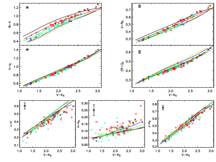
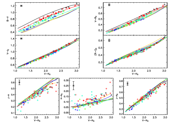
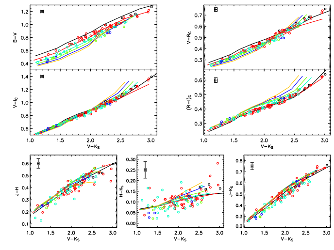
3.2 Comparison of model and empirical colours

Figure 6: Lines represent the colour-colour relations derived from the empirical colour-temperature calibrations of Ramírez & Meléndez (2005a). Points correspond to our sample of stars. Colours and metallicity ranges for lines and points are same as in Figure 2 except that metallicities of +0.5 have been excluded since the empirical relations do not hold in that range. In the optical the empirical relations fit the observed colours with an accuracy comparable to the theoretical ones (compare with Figure 2). However in the infrared, for metallicities around the solar, empirical relations oscillate in reproducing the observed trend. This is especially interesting in light of the puzzling infrared colours of the Sun and the shifts required to cool down the temperature scale as discussed in Section 5.

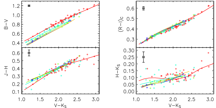
All our colour-colour comparisons are as a function of $(V-K_{S})$. This approach highlights the behaviour of colours as function of temperature and also make more straightforward the comparison with the empirical colour-temperature relations in the Section 3.3. $(V-K_{S})$ has a large range compared to its observational uncertainty and it is known to be metallicity insensitive (e.g. Bell & Gustafsson 1989 and Figure 13).

All models are found to be in good overall agreement with the observations. In particular, the improvement in the input physics of the latest ATLAS9 and MARCS models show excellent agreement with the optical data (Figures 2 and 3) and as good as the semi-empirical libraries in the other bands, so that we do not find any specific reason to prefer the use of semi-empirical libraries.

We expect the IR colours to be very important both in observational terms and in theoretical modelling. Recently, Frémaux et al. (2006) have presented a detailed comparison of theoretical spectra (from the NeMo library) in $H$ band with observed stellar spectra at resolution around 3000. They show that in the infrared range, although the overall shape of the observed flux distribution is matched reasonably well, individual features are reproduced by the theoretical spectra only for stars earlier than mid F type. For later spectral types the differences increase and theoretical spectra of K type stars have systematically weaker line features than those found in observations. They conclude that these discrepancies stem from incomplete data on neutral atomic (and to a minor extent to molecular) lines.

The synthetic optical colours agree well with observed ones and models also predict the correct metallicity dependence. In the infrared, models fit satisfactorily the overall trend given by the observed colours, however the scatter in the data prevent firm conclusions. In $J-H$ and $J-K_{S}$ the model colours seem to be slightly offset by $\sim 0.05$ mag, whereas in $H-K_{S}$ the disagreement is somewhat smaller though it depends on the models considered and it seems to increase going to cooler temperatures.

3.3 Empirical colour-temperature relations compared to observed and synthetic photometry

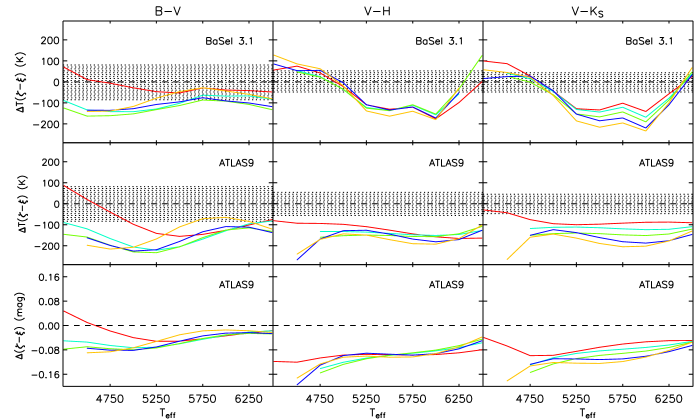
We now compare empirical colour-temperature calibrations with synthetic and observed photometry. To this purpose, we use the calibration recently proposed by Ramírez & Meléndez (2005a).

In Fig. 5 we plot the difference between the temperature of the model atmospheres (BaSel 3.1 and ATLAS9) and the temperature expected for their colours according to the empirical Ramírez & Meléndez relations. Interestingly, all models fail to set onto the empirical temperature scale being at least 100 K hotter in optical and infrared colours. The disagreement is particularly strong at low metallicity as noticed by Ramírez & Meléndez. The semi-empirical libraries of Lejeune et al. (1997) and Westera et al. (2002), though in principle optimized to reproduce colour-temperature relations, provide only a marginal improvement with respect to the latest purely theoretical ATLAS9 and MARCS libraries. The temperature offset can be translated into a shift in colours needed to set the models onto the empirical scale. This is done for the ATLAS9 model in the last row of Figure 5; in terms of colours, the mismatch corresponds to $\sim 0.1$ mag.

Empirical calibrations depend on metallicities and colour indices only. The adopted absolute calibration can not be the main cause of the disagreement since all colours (in the optical) scale accordingly. In the optical the adopted Vega model that sets the absolute calibration has been accurately tested by Bohlin & Gilliland (2004) (see Appendix A). Although we adopt a different absolute calibration in the optical and in the infrared (see Appendix A), this could at most affect the colour-metallicity-temperature relations in $V-J$, $V-H$ and $V-K_{S}$. Even using in the infrared the same absolutely calibrated Vega model adopted in the optical does not eliminate the disagreement and offsets of 100 K still persist.

We have also verified that the choice of zero-points plays a negligible role: differences in the optical zero-points based on Vega or on the average of Vega and Sirius (see Appendix A) lead to mean temperature differences of 10 to 30 K. Besides being much smaller than the uncertainty in the colour-temperature relations, such differences go in the direction of worsening the disagreement.

As to the IR zero-points, we checked their effects by generating IR synthetic magnitudes in the TCS and Johnson system (where the Vega zero-points are different from those deduced from 2MASS photometry) and compared the model predictions to the Alonso et al. (1996a) empirical calibration in these bands; typical discrepancies of more than 100 K still persist.

The causes for the discrepancy must therefore be model deficiencies and/or inaccuracies in the adopted empirical relations.

In fact we caution that also empirical relations may hide some inadequacies. For instance, the Ramírez & Meléndez calibration predicts slightly bluer colours for the Sun than the recent completely empirical determination of Holmberg, Flynn & Portinari (2006). We can also combine and invert the Ramírez & Meléndez’ colour-temperature calibrations, to derive the corresponding empirical colour-colour relations and compare them to the observed colours for our sample of stars. Interestingly the agreement is not always good: the solar metallicity is slightly offset with respect to the data in $(R-I)_{C}$ band and in the infrared tends to oscillate (see Figure 6). This underlines that there is still room for improvement also in the empirical relations.

4 An implementation of the IRFM

In this section we have used $BV(RI)_{C}JHK_{S}$ photometry as the basic observational information to derive bolometric fluxes and effective temperatures of our 104 G and K dwarfs. Our approach follows the InfraRed Flux Method (IRFM) used in the extensive work of Alonso, Arribas & Martínez-Roger (1995, 1996b). Ours is a new independent implementation of the IRFM, applied to our 104 G and K type dwarfs.

Our implementation differs from Alonso et al (1995, 1996), as we base its absolute calibration on a synthetic spectrum of Vega (as described in detail in Appendix A) rather than on semi-empirical measurements (Alonso, Arribas & Martínez-Roger, 1994). The use of absolutely calibrated synthetic spectra rather than ground-based measurements traces back to Blackwell et al. (1990, 1991a), who concluded that atmospheric models of Vega offered higher precision than observationally determined absolute calibrations. This approach has been adopted in the extensive work of Cohen and collaborators and also Bessell, Castelli & Plez (1998), who concluded that model atmospheres are more reliable than the near-infrared absolute calibration measurements. Models are nowadays sophisticated enough to warrant detailed comparisons between observation and theory and the latest space based measurements confirm the validity of the adopted absolute calibration (see Appendix A). We also differ from the recent work of Ramírez & Meléndez (2005b) in using the most recent model atmospheres and absolute calibration available. Furthermore we use only direct observational data, explicitly avoiding the use of colour calibrations from previous studies to infer the bolometric luminosity.

Following Alonso et al. (1995), the flux outside the wavelength range covered by our photometry has been estimated using model atmospheres. Since the percentage of $F_{bol}$ measured in the directly observed bands range from $\sim 70$% to $\sim 85$% depending on the star, the dependence of the estimated bolometric flux on the model is small.

In Section 4.1 and 4.2 we give a detailed description of our implementation of the IRFM, mainly following the formulation and terminology adopted by Alonso et al. (1995, 1996b).

Our procedure can be summarized as follows. Given the metallicity, the surface gravity (assuming $\log(g)=4.5$ for all our dwarfs, see Section 3.1) and an initial estimate for the temperature of a star, we have interpolated over the grid of model atmospheres to find the spectrum that best matches these parameters. This spectrum is used to estimate that fraction of the bolometric flux outside our filters $(BV(RI)_{C}JHK_{S})$, i.e. the ‘bolometric correction’. The bolometric flux is determined from the observations, including the bolometric correction. A new effective temperature $T_{\mathrm{e}ff}$ can be computed by means of the IRFM. This temperature is used for a second interpolation over the grid, and the procedure is iterated until the temperature converges to within 1 K (typically within 10 iterations).

We have tested the results using ATLAS9, MARCS, BaSel 2.1 and 3.1 libraries. A detailed discussion on the the dependence on the adopted model is given in Section 4.3.

In the following sections we describe our implementation of the IRFM effective temperature scale.

4.1 Bolometric fluxes

As mentioned above, we use grids of synthetic spectra to bootstrap our IRFM. The grids of synthetic spectra all have a resolution of 250 K in temperature whereas the resolution in metallicity depends on the library, but with typical steps of 0.25 or 0.50 dex.

For any given star of overall metallicity [M/H] (c.f. Eq. (1), we interpolate over the grid of synthetic spectra in the following way. First, we use the $T_{\mathrm{e}ff}:(V-K)$ calibration of Alonso et al. (1996a) to obtain an initial estimate of the effective temperature $T_{\mathrm{e}ff,0}$ of the star. Then we linearly interpolate in $\log(T_{\mathrm{e}ff})$ bracketing our temperature estimate $T_{\mathrm{e}ff,0}$ at two fixed values of metallicity, which bracket the measured [M/H] of the star. A third linear interpolation is finally done in metallicity in order to obtain the desired synthetic spectrum.

Having obtained the spectrum $F(\lambda)$ that better matches the physical parameters of the star, for any given band $\zeta$ (running from $B$ to $K_{S}$), we convolve it through the transmission curve $T_{\zeta}(\lambda)$ of the filter and associate the resulting $\mathcal{F}_{\zeta}(\textrm{model})$ with its effective wavelength $\lambda_{\mathrm{e}ff}$ (see Appendix B).

We then compute the flux covered by the passbands $B$ to $K_{S}$ for the model star ($\mathcal{F}_{B-K_{S}}(\textrm{model})$). When the latter is compared with the bolometric flux for the same model star ($\mathcal{F}_{Bol}(\textrm{model})$) we can obtain an estimate of the fraction of the flux $\mathcal{C}$ encompassed by our filters:

$$\mathcal{C}=\frac{\mathcal{F}_{B-K_{S}}(\textrm{model})}{\mathcal{F}_{Bol}(\textrm{model})}.$$ (3)

We now have the correction factor $1/\mathcal{C}$ for the missing flux of a given star, we use its observed $BV(RI)_{C}JHK_{S}$ magnitudes ($m_{\zeta}$) to calculate the flux as it arrives on the Earth:

$$\mathcal{F}_{\zeta}(\textrm{Earth})=\mathcal{F}_{\zeta}^{std}(\textrm{Earth})10^{-0.4(m_{\zeta}-m_{\zeta}^{std})},$$ (4)

where $\mathcal{F}_{\zeta}^{std}(\textrm{Earth})$ is the absolute calibrated flux on the Earth of the standard star and $m_{\zeta}^{std}$ is its observed magnitude. The observed magnitudes and the absolute calibration of the standard star are those given in Table 13 and 14 respectively and play a key role in determining both bolometric flux and effective temperature as we discuss in Section 4.4.3.

The flux at the Earth for each band is once again associated with the corresponding effective wavelength of the star, and a simple integration leads to $\mathcal{F}_{B-K_{S}}(\textrm{Earth})$. The latter is then divided by the $\mathcal{C}$ factor as defined in eq. (3) in order to obtain the bolometric flux measured on the Earth $\mathcal{F}_{Bol}(\textrm{Earth})$.

4.2 Effective Temperatures

The effective temperature $T_{\mathrm{e}ff}$ of a star satisfies the Stefan-Boltzman law $\mathcal{F}_{Bol}=\sigma T_{\mathrm{e}ff}^{4}$, where $\mathcal{F}_{Bol}$ is the bolometric flux on the surface of the star. Only the bolometric flux on the Earth is measurable, and we must take into account the angular diameter ($\theta$) of the star. Thus:

$$\mathcal{F}_{Bol}(\textrm{Earth})=\left(\frac{\theta}{2}\right)^{2}\sigma T_{\mathrm{e}ff}^{4}.$$ (5)

The way to break the degeneracy between effective temperature and angular diameter in the previous equation is provided by the InfraRed Flux Method (Blackwell & Shallis 1977; Blackwell, Shallis & Selby 1979; Blackwell, Petford & Shallis 1980). The underlying idea relies on the fact that whereas the bolometric flux depends on both angular diameter and effective temperature (to the fourth power), the monochromatic flux in the infrared at Earth – $\mathcal{F}_{\lambda_{\textrm{\tiny{IR}}}}(\textrm{Earth})$ – depends on the angular diameter but only weakly (roughly to the first power) on the effective temperature:

$$\mathcal{F}_{\lambda_{\textrm{\tiny{IR}}}}(\textrm{Earth})=\left(\frac{\theta}{2}\right)^{2}\phi(T_{\mathrm{e}ff},g,\lambda_{\textrm{\tiny{IR}}}),$$ (6)

where $\phi(T_{\mathrm{e}ff},g,\lambda_{\textrm{\tiny{IR}}})$ is the monochromatic surface flux of the star. The ratio $\mathcal{F}_{Bol}(\textrm{Earth})/\mathcal{F}_{\lambda_{\textrm{\tiny{IR}}}}(\textrm{Earth})$ defines what is known as the observational $R$-factor ($R_{obs}$), where the dependence on $\theta$ is eliminated. In this sense the IRFM can be regarded as an extreme example of a colour method for determining the temperature. By means of synthetic spectra it is possible to define a theoretical counterpart ($R_{theo}$) on the surface of the star, obtained as the quotient between the integrated flux ($\sigma T_{\mathrm{e}ff}^{4}$) and the monochromatic flux in the infrared $\mathcal{F}_{\lambda_{\textrm{\tiny{IR}}}}(\textrm{model})$.

The basic equation of the IRFM thus reads:

$$\frac{\mathcal{F}_{Bol}(\textrm{Earth})}{\mathcal{F}_{\lambda_{\textrm{\tiny{IR}}}}(\textrm{Earth})}=\frac{\sigma T_{\mathrm{e}ff}^{4}}{\mathcal{F}_{\lambda_{\textrm{\tiny{IR}}}}(\textrm{model})}$$ (7)

and can be immediately rearranged to give the effective temperature, eliminating the dependence on $\theta$.

The monochromatic flux $\mathcal{F}_{\lambda_{\textrm{\tiny{IR}}}}(\textrm{Earth})$ is obtained from the infrared photometry using the following relation:

$$\mathcal{F}_{\lambda_{\textrm{\tiny{IR}}}}(\textrm{Earth})=q(\lambda_{\textrm{\tiny{IR}}})\;\mathcal{F}_{\lambda_{\textrm{\tiny{IR}}}}^{std}(\textrm{Earth})\;10^{-0.4(m_{\textrm{\tiny{IR}}}-m_{\textrm{\tiny{IR}}}^{std})},$$ (8)

where $q(\lambda_{\textrm{\tiny{IR}}})$ is a correction factor to determine monochromatic flux from broad-band photometry, $m_{\textrm{\tiny{IR}}}$ is the infrared magnitude of the target star, $m_{\textrm{\tiny{IR}}}^{std}$ and $\mathcal{F}_{\lambda_{\textrm{\tiny{IR}}}}^{std}(\textrm{Earth})$ are the magnitude and the absolute monochromatic flux of the standard star in the same infrared band (see Table 13 and 14). For the standard and the target star $\lambda_{IR}$ refers to their respective effective wavelength in the given infrared band, as we discuss in more detail, together with the definition of the $q$–factor, in Appendix B.

The IRFM is often applied using more than one infrared wavelength and different $T_{\mathrm{e}ff}$ are obtained for each wavelength. Ideally, the derived temperatures should of course be independent of the monochromatic wavelength used. In our case we have used $J,H,K_{S}$ photometry and the corresponding effective wavelengths.

We have tested the systematic differences in temperatures, luminosities and diameters obtained when only one infrared band at a time is used for the convergence of the IRFM. The results are shown in Figure 7.

Figure 7: Comparison of effective temperatures, angular diameters and bolometric luminosities obtained in the three infrared bands used. Angular diameters have been scaled using the stellar parallaxes from Hipparcos, although the parallaxes do not affect the comparison since all bands scale accordingly. The luminosities of the stars are in good agreement across all the IR bands (because luminosity is also tied down by the optical data as discussed in the text). Offsets of this size are likely to stem from the difficulties in setting the zero points of the absolute calibration. Horizontal and diagonal lines with slope 1 are intended to guide the eye.

The $J$ band returns temperatures that are systematically cooler than those found from $K_{S}$, which translates into greater angular diameters. The $H$ band, returns temperatures that are systematically hotter and therefore smaller angular diameters than in $K_{S}$. These systematic differences do not appear to depend on the temperature range, at least between 4500–6500 K.

The systematic offsets could be traced back to the absolute calibration in different bands. We further point out that for the sake of this test, the convergence on $T_{\mathrm{e}ff}$ in the IRFM is required in one band only and in Figure 7 the differences are thus exaggerated. The discrepancy can reach a few percent in temperatures and diameters, whereas for bolometric luminosities is usually within 2% though it increases with increasing temperature (Figure 7). This is due to the fact that the derived bolometric luminosity is constrained from the full optical and infrared photometry and absolute calibration, whereas for temperature and angular diameter, when relying on one IR band only, the absolute calibration in that band strongly affects the results.

Alonso et al. (1996b) concluded that the consistency of the three infrared bands they used ($J,H,K$) was good over 4000 K, but decided to use only $H$ and $K$ below 5000 K and only $K$ below 4000 K and basically the same is done by Ramírez & Meléndez (2005b). We have decided to use the temperature returned in all three bands also below 5000 K, since systematic differences are not too large even below 5000 K, the cooler temperatures in $J$ band being compensated by the hotter ones in $H$ band.

At each iteration the temperature used for the convergence is the average of the three IR values weighted with the inverse of their errors “j_,” “h_,” and “k_msigcom”. This temperature is then used to select a new model interpolating over the grid of synthetic spectra as described in Section 4.1 and a new bolometric flux and temperature are then computed. The procedure is iterated until the average temperature converges within 1 K. As can be appreciated from Figure 8 the systematic differences between the three bands are much reduced. Ideally the ratio of the temperatures determined in the three bands should be unity. The three mean ratios $T(K_{S})/T(J)$, $T(K_{S})/T(H)$ and $T(H)/T(J)$ together with their standard deviations, are 1.0069 ($\sigma=0.77$%), 0.9943 ($\sigma=0.82$%) and 1.0126 ($\sigma=0.89$%) and this also confirms the quality of the adopted absolute calibration. The mean standard deviation for the three infrared temperatures is 39 K, reflecting the different band sensitivity to the temperature, the effect of the absolute calibration in different bands as well as the observational errors in the infrared photometry.

Figure 8: Differences as a function of temperature between the final adopted values and those obtained in each $\zeta=J,H,K_{S}$ band when the convergence is done averaging the three IR values.

4.3 Internal accuracy and dependence on the adopted library

We have probed the accuracy and the internal consistency of the procedure described in Sections 4.1 and 4.2 generating synthetic magnitudes in the range $4250\leq T_{\mathrm{e}ff}\leq 6500$ and $-2.0\leq\textrm{[Fe/H]}\leq 0.5$ and testing how the adopted method recovers the temperatures and luminosities of the underlying synthetic spectra. The accuracy is excellent given that in all three infrared bands the IRFM recovers the right temperature within 1 K and the bolometric luminosity (i.e. the theoretical value $\sigma T_{\mathrm{e}ff}^{4}$) within 0.1% and 0.04% for the ATLAS and MARCS models respectively, i.e. at the level of the numerical accuracy of direct integration of the bolometric flux from the spectra. This confirms that the interpolation over the grid introduces no systematics and even a poor initial estimate of the temperature does not affect the method.

We expect the dependence of the results on the adopted synthetic library to be small, since most of the luminosity is actually observed photometrically and the model dependence for the $q$-factor and $R_{theo}$ (see Section 4.2) is weak because we are working in a region of the spectrum largely dominated by the continuum. The method is in fact more sensitive to the adopted absolute calibration that governs $R_{obs}$.

The principal contributor to continuous opacity in cool stars is due to $\textrm{H}^{-}$. Blackwell, Lynas-Gray & Petford (1991b) have shown that by using more accurate opacities with respect to previous work, temperatures increased by 1.3% and angular diameters decreased up to 2.7%, the effect being greatest for cool stars. Even though the dependence of the results on the adopted synthetic library is small, the use of absolute calibrations derived using the most up-to-date model atmospheres (see Appendix A) is of primary importance. Though we use a great deal of observational information, the new opacity distribution function (ODF) in the adopted grid of model atmospheres is particularly important. With respect to the more accurate but computationally time consuming opacity sampling (OS), older ODF models can underestimate the IR flux by few percent, translating into cooler effective temperatures (Grupp, 2004a). Likewise, the better opacities in the UV lead to an increased flux in the visual and infrared region. This directly affects the ratio between the bolometric and monochromatic flux used for the Infrared Flux Method (see Section 4.2), so that the latest model atmosphere have to be preferred (Megessier 1994; 1998).

For all our 104 G–K dwarfs we have tested how the recovered parameters change by using ATLAS9, MARCS, BaSel 2.1 and 3.1 libraries. The comparison in temperatures, luminosities and angular diameters is shown in Figure 9.

Figure 9: Comparison between final effective temperatures, bolometric luminosities and angular diameters for our sample stars, when different synthetic libraries (with respect to ATLAS9) are used.

The ATLAS9 and MARCS models show a remarkably good agreement through all the temperature range, with differences in the temperature that never exceed a few degrees (or 0.2%) and those in the bolometric luminosities and the angular diameters being always within 1%. Though not a proof of the validity of the models, it is very encouraging that the sophisticated physics implemented in independent spectral synthesis codes shows such a high degree of consistency.

The BaSel models show bigger differences with respect to ATLAS9. The BaSel 2.1 model tends to give slightly hotter temperatures, higher luminosities and smaller angular diameters when compared to ATLAS9, though the systematic is oscillating (reflecting the underlying continuum adjustments of the semi-empirical BaSel libraries).

We conclude by noting that in the range of temperatures and luminosities studied the dependence of our results on the adopted model never exceeds a few percent and for the latest models (MARCS and ATLAS9) the agreement is well within 1%. Hence we will only present and discuss results based on ATLAS9 in the following.

4.4 Evaluation of the errors: rounding up the usual suspects

Though the IRFM is known to be one of the most accurate ways of determining stellar temperatures without direct angular diameter measurements, its dependence on the observed photometry and metallicities, on the absolute calibration adopted and on the library of synthetic spectra make the evaluation of the errors not straightforward. In this work we have proceeded from first principles and made use of high accuracy observations only, thus facilitating the estimation of errors and possible biases. Since we made use of photometric measurements in many bands, we expect the dependence on photometric errors to be rather small, small random errors in different bands being likely to compensate each other. We have also shown in the previous section that when the latest model atmospheres are adopted, the model dependence is below the one percent level. The effect of the absolute calibration can be regarded as a systematic bias; once the absolute calibration in different bands is chosen, all temperatures scale accordingly. As we show in Appendix A the adopted absolute calibration has been thoroughly tested.

4.4.1 Photometric observational error

The photometric errors in different bands as well as errors in metallicity are likely to compensate each other. In order to check this, for each star we have run 1000 MonteCarlo simulations, assigning each time random errors in $BV(RI)_{C}JHK_{S}$ and [Fe/H]. The errors have been assigned with a normal distribution around the observed value and a standard deviation of 0.01 mag in $BV(RI)_{C}$ and of “j_,” “h_,” “k_msigcom” in $JHK_{S}$. Errors in [Fe/H] are those given in the papers from which we have collected abundances.

The standard deviation of the resulting temperatures obtained from the MonteCarlo for each star is typically 11 K and never exceeds 19 K. Bolometric luminosities have a mean relative error of only 0.5% and never exceeding 0.8%; for angular diameters the mean error sets to 0.4% and never exceeds 0.5%.

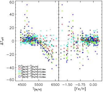
4.4.2 Metallicity and surface gravity dependence

The interpolation within the grid of synthetic spectra is as a function of [M/H]. We have checked the effect of $\alpha$–elements by making the interpolation as a function of [Fe/H] instead, finding very little differences in the derived fundamental parameters around the solar values. At lower metallicities the effect of the $\alpha$–elements start to be important as expected (Figure 10). The effect is in any case, always within 20 K in $T_{\mathrm{e}ff}$ and within 2% in bolometric luminosity and $\theta$.

Figure 10: Differences between temperatures, bolometric luminosities and angular diameters when the [M/H] or [Fe/H] are used.

Spectroscopic metallicities have typical errors well within 0.10 dex. As we show in Figure 11 a change of few dex in metallicity has almost no effect on the resulting temperatures around the solar values, but at lower metallicities systematic errors of 0.10–0.20 dex in [Fe/H] can introduce biases up to 40 K. This is an important point when using large surveys with photometric metallicities that have typical errors above 0.10 dex.

Figure 11: Effect of errors in metallicities on the resulting temperatures.

The dependence on the adopted surface gravity is very mild for dwarf stars. We have verified that a change of $\pm 0.5$ dex in $\log(g)$ implies differences that never exceed $\sim 30$ K in temperature and well within 1% for bolometric fluxes and angular diameters.

4.4.3 Systematic error in the absolute calibration

The errors in the adopted magnitudes and absolute calibrations of Vega in different bands can be regarded as a systematic bias, since once they are selected, the recovered temperatures, luminosities and angular diameters scale accordingly. Errors in the observed $BV(RI)_{C}$ magnitudes of Vega are around 0.01 mag whereas the uncertainties in $JHK_{S}$ magnitudes given by Cohen et al. (2003) are within a few millimag. As for the random errors on the photometric zero-points, it is very likely that uncertainties in Vega’s magnitudes compensate each other.

On the other hand, the uncertainties in the adopted absolute calibration mainly come from the uncertainty in the flux of Vega at 5556 Å. Since the absolute calibration in all bands scales accordingly (even though we have used slightly different approaches in optical and infrared, see Appendix A), we evaluate the systematic error in temperatures for the worst case scenario, i.e. when all errors correlate to give systematically higher or lower fluxes. The uncertainties adopted are those given in Table 14. The results are shown in Figure 12.

Figure 12: Effect of the absolute calibration being systematically brighter (circles) or fainter (squares) when uncertainties given in Table 14 correlate. Translated into magnitudes it corresponds to a mean shift of Vega’s zero-points of $\pm 0.01$ mag in the optical and $\pm 0.02$ mag in the infrared.

Finally, a detailed comparison with data from satellites validate within the errors the adopted calibration, though it seems to suggest that infrared fluxes should be brightened by 1% at most (see Appendix A). If so, the resulting temperatures would cool down by 10 to 30 K and luminosities and angular diameters would increase on average by 0.2% and 0.7%, respectively.

4.4.4 The final error budget

The primary estimate for errors in $T_{\mathrm{e}ff}$ is from the scatter in the temperature deduced from $J$, $H$ and $K_{S}$ bands that reflects photometric errors as well as differences in the corresponding absolute calibration (see Section 4.2). As regards the uncertainties discussed in Sections 4.4.2 and 4.4.1, they are of the same order and we quadratically sum them to the standard deviation in the resulting $J$, $H$ and $K_{S}$ for a fair estimate of the global errors on temperatures.

The uncertainties of the bolometric luminosities mostly depend on the photometry that accounts for $\sim$ 70–85% of the resulting luminosity. The errors from the observations have been estimated by summing in quadrature those from the MonteCarlo simulation (Section 4.4.1) to those due to a change of $\pm 0.5$ dex in $\log(g)$.

Finally, for the resulting angular diameters we propagate the errors in temperature and luminosity from equation 5. The mean internal accuracy of the resulting temperatures is of 0.8%, that of the luminosities of 0.5% and that of the angular diameters of 1.7%.

There are possible systematic errors coming from the adopted absolute calibration. As can be seen from Figure 12 such uncertainties give an additional mean error of 0.3% in temperature and 1.2% in luminosity that translate into an additional systematic error of 0.7% in angular diameters. A summary of the uncertainties is given in Table 2.

Table 2: Mean accuracy of the derived fundamental stellar parameters. Notice that either the systematics given here, either those shown in Figure 12 are determined according Table 14 and do not account for possible (and only indicative) shifts in Vega’s zero-points as a consequence of its rapidly rotating nature (see Appendix A).

	Internal accuracy	Systematics
$T_{\mathrm{e}ff}$	0.8%	0.3%
$\mathcal{F}_{Bol}$	0.5%	1.2%
$\theta$	1.7%	0.7%

Figure 13: Empirical colour-temperature relations. Circles are for stars with [Fe/H] $\leq-0.5$, crosses for stars with [Fe/H] $>-0.5$. Red (cyan) continuous lines are our (Ramírez & Meléndez 2005a) fitting formulae at solar metallicity. Dotted lines are for [Fe/H] $=-1$. In the infrared, for stars with $T_{\mathrm{e}ff}$ below 5000 K the Ramírez & Meléndez (2005a) calibration shows a larger metallicity dependence than indicated by our data.

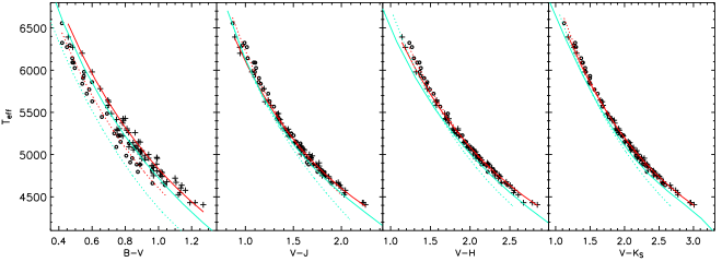
4.5 Colour-temperature-metallicity fitting formulae

To reproduce the observed relation $T_{\mathrm{e}ff}$ vs. colour and to take into account the effects of different chemical compositions, the following fitting formula has been adopted (e.g Alonso et al. 1996a, Ramírez & Meléndez 2005a, Masana et al. 2006):

$$\theta_{\mathrm{e}ff}=a_{0}+a_{1}X+a_{2}X^{2}+a_{3}X\textrm{[Fe/H]}$$

$$\phantom{\theta_{\mathrm{e}ff}=}+a_{4}\textrm{[Fe/H]}+a_{5}\textrm{[Fe/H]}^{2},$$ (9)

where $\theta_{\mathrm{e}ff}=5040/T_{\mathrm{e}ff}$, $X$ represents the colour and $a_{i}$ ($i=1,$…,$5$) the coefficients of the fit. In the iterative fitting, points departing more than $3\sigma$ from the mean fit were discarded (very few points ever needed to be removed). All our relations were adequately fit by simple polynomials, and we did not need to got to higher orders in $X$ to remove possible systematics as function of the metallicity (as in Ramírez & Meléndez, 2005a, who covered a much wider range in temperature than we do here).

Figure 13 shows the colour-temperature relations in different bands. The coefficients of the fits, together with the number of stars used, the range of applicability and the standard deviations are given in Table 3. Note that the very small scatter in the relations reflects the high-quality and homogeneity of the input data.

Table 3: Coefficients and range of applicability of the colour-temperature relations.

Colour	Metallicity range	Colour range	$a_{0}$	$a_{1}$	$a_{2}$	$a_{3}$	$a_{4}$	$a_{5}$	$N$	$\sigma(T_{\mathrm{e}ff})$
$B-V$	$\left[-1.87,0.34\right]$	$\left[0.419,1.270\right]$	0.5121	0.5934	$-$0.0618	$-$0.0319	$-$0.0294	$-$0.0102	103	54
$V-R_{C}$	$\left[-1.87,0.34\right]$	$\left[0.249,0.755\right]$	0.4313	1.5150	$-$0.7723	$-$0.0950	0.0179	$-$0.0033	101	55
$(R-I)_{C}$	$\left[-1.87,0.34\right]$	$\left[0.268,0.640\right]$	0.2603	2.3449	$-$1.4897	$-$0.1149	0.0641	0.0023	104	70
$V-I_{C}$	$\left[-1.87,0.34\right]$	$\left[0.517,1.395\right]$	0.3711	0.8994	$-$0.2467	$-$0.0545	0.0393	$-$0.0010	101	49
$V-J$	$\left[-1.87,0.34\right]$	$\left[0.867,2.251\right]$	0.4613	0.4118	$-$0.0473	$-$0.0356	0.0535	0.0012	104	30
$V-H$	$\left[-1.87,0.34\right]$	$\left[1.144,2.847\right]$	0.4797	0.3059	$-$0.0252	$-$0.0196	0.0426	0.0036	99	25
$V-K_{S}$	$\left[-1.87,0.34\right]$	$\left[1.124,3.010\right]$	0.4609	0.3069	$-$0.0263	$-$0.0145	0.0275	0.0006	103	21

$N$ is the number of stars employed for the fit after the $3\sigma$ clipping and $\sigma(T_{\mathrm{e}ff})$ the final standard deviation of the proposed calibrations.

5 The temperature scale: some like it hot

In this section we test our IRFM in a number of ways. Firstly, we compare its predictions to empirical data for the Sun and solar analogs. Secondly, we compare our predicted angular diameters to recent measurements with large telescope interferometers for a small sample of G and K dwarfs. Thirdly, we compare our system to other temperature scales for G and K dwarfs in the literature.

Overall, we find that our scale is in good agreement with other scales though some puzzles remain. We make some suggestions for further work.

5.1 The Sun and solar analogs

While the temperature, the luminosity and the radius of the Sun are known with great accuracy, its photometric colours can only be recovered indirectly. Recently, Holmberg et al. (2006) have provided colour estimates for the Sun based on those of solar analogs. Another way to obtain colours of the Sun levers synthetic photometry, convolving empirical or model spectra of the Sun with filter response functions (e.g. Bessell et al. 1998). Both methods lead to estimated colours that have typical uncertainties of a few 0.01 mag. Though this prevents the use of the Sun as a direct calibrator of the temperature scale, it is still useful to compare to its estimated colours.

5.1.1 The colours of the Sun

We have computed synthetic solar colours from the solar reference spectrum of Colina et al. (1996) which combines absolute flux measurements (from satellites and from the ground) with a model spectrum longward of 9600 Å. This spectrum, together with those of three solar analogs, is available from the CALSPEC library. According to Colina et al. (1996), the synthetic optical and near-infrared magnitudes of the absolutely calibrated solar reference spectrum agree with published values to within 0.01-0.03 mag.

Recently, two new composite solar spectra extending up to 24000 Å have been assembled by Thuillier et al. (2004) based on the most recent space-based data. The accuracy in the UV-visible and near IR is of order 3%. The two solar spectra correspond to moderately high and moderately low solar activity conditions, although the effect of activity on the resulting synthetic colours is at or below the millimag level, except for $U-B$ (0.003 mag). Such small differences could be due to the solar spectral variability (which increases toward shorter wavelengths), the accuracy of the measurements or both. In what follows we adopt therefore the pragmatic approach of averaging the colours returned by the two spectra and we generically refer to the results as the Thuillier et al. (2004) spectrum.

We have also computed the theoretical magnitudes and colours of the Sun predicted by the latest Kurucz and MARCS synthetic spectra. Magnitudes and colours computed from the aforementioned solar spectra are given in Table 4 together with the empirical colours of Holmberg et al. (2006).

Table 4: Magnitudes and colours of the Sun compared to theoretical colours and those deduced using our temperature scale.

$V$	$U-B$	$B-V$	$V-R_{C}$	$(R-I)_{C}$	$V-J$	$V-H$	$V-K_{S}$	Ref.
…	$0.173\pm 0.064$	$0.642\pm 0.016$	$0.354\pm 0.010$	$0.332\pm 0.008$	$1.151\pm 0.035$	$1.409\pm 0.035$	$1.505\pm 0.041$	(a)
$-$26.742	0.131	0.648	0.373	0.353	1.165	1.483	1.555	(b)
$-$26.743	0.146	0.635	0.374	0.358	1.189	1.528	1.613	(c)
$-$26.740	0.101	0.645	0.358	0.349	1.162	1.495	1.556	(d)
$-$26.746	0.120	0.658	0.370	0.350	1.166	1.483	1.555	(e)
$-$26.753	0.188	0.633	0.360	0.345	1.154	1.485	1.547	(f)
…	…	0.651	0.356	0.330	1.150	1.459	1.546	(g)

(a) Holmberg et al. (2006); (b) Colina et al. (1996); (c) Thuillier et al. (2004) (d) ATLAS9 ODFNEW with Grevesse & Sauval solar abundances; (e) Kurucz 2004 model with resolving power 100000; (f) MARCS; (g) our temperature scale.

Although we have not looked at stellar $U$ magnitudes in this study, for completeness with the work of Holmberg et al. (2006) we have generated synthetic magnitudes in this band too. However, in what follows we focus our discussion from $B$ to $K_{S}$ band (for a discussion of the theoretical solar $U-B$ colour see e.g. Grupp 2004b and references therein). We have used only Vega to set the zero points. The differences in the resulting colours when also Sirius is used for the optical bands are given in Appendix A and tend to make the solar $B-V$ even redder. Assuming no deficiencies in the synthetic spectra, the uncertainties in the derived colours are entirely due to the uncertainties in the adopted zero points, i.e. in the order of $\sim$ 0.01 mag.

The CALSPEC and Thuillier et al. (2004) spectra are already absolutely calibrated for a distance of 1 AU. For the absolute calibration of the Kurucz and MARCS solar spectra, we also adopt a distance of 1 AU. The synthetic spectra have a temperature $T_{\odot}=5777\;\textrm{K}$ and we adopt $L_{\odot}=3.842\times 10^{33}\,\textrm{erg s}^{-1}$ (Bahcall, Serenelli & Basu 2005) from which we deduce $R_{\odot}=\sqrt{L_{\odot}/4\pi\sigma T_{\odot}^{4}}$ to be used for the absolute calibration. Proceeding this way we can immediately compare the recovered temperatures and luminosities by means of the IRFM (see Table 5) with those given above. The effect of the absolute calibration of the solar spectra is immediately seen in the deduced value of $V$ and reflects in the recovered luminosity whereas the temperature depends on the colours only.

An influential direct $V$ measurement of the Sun is that of Stebbins & Kron (1957) to which Hayes (1985) claimed a further 0.02 mag correction for horizontal extinction. Using recent standard $V$ magnitudes for the Stebbins & Kron (1957) comparison G dwarfs returns for the Sun $V=-26.744\pm 0.015$, which becomes $V=-26.76\pm 0.02$ after accounting for the Hayes correction (Bessell, Castelli & Plez 1998). The values deduced using composite and synthetic spectra are closer to the measurements of Stebbins & Kron but fully within the error bars of the Hayes’ value. Note that through the year the variation of the solar distance due to the ellipticity of the Earth’s orbit corresponds to a $V$ difference of $\pm 0.035$ mag.

In the optical bands synthetic and composite colours show a remarkably good agreement with the recent empirical determination, differences being at most 0.01–0.02 mag and therefore within the error bars. Synthetic and composite spectra also confirm the redder $B-V$ colour with respect to the determination of Sekiguchi & Fukugita (2000) ($B-V=0.626$) and Ramírez & Meléndez (2005a) ($B-V=0.619$), though the Thuillier et al. (2004) spectrum is slightly bluer than the Neckel & Labs (1984) measurements used in the Colina et al. (1996) composite spectrum. Using the empirical value of $B-V=0.642$ in the Ramírez & Meléndez (2005a) colour-temperature relation implies a temperature of the Sun of 5699 K, therefore suggesting the need of a hotter temperature scale for this colour. Such an offset is of the same order of those found in Section 3.3 for optical and infrared bands.

In the infrared, the only directly measured spectrum is that of Thuillier et al. (2004). It is much redder than the empirical determination of Holmberg et al. (2006) and also the model spectra. As concerns the other models, $J$ band shows good agreement with the empirical determination. Though a systematic offset of $\sim$ 0.01 mag appears, it is fully within the error bars. The $H$ and $K_{S}$ bands show larger systematic differences in the order of 0.08 and 0.05 mag respectively as Figure 5 already suggests. Such large differences are not easily understood in terms of model failures. Interestingly, an offset of 0.075 mag in the $H$ band zero-point given by the 2MASS has also been claimed by Masana et al. (2006) to constrain a set of solar analogs to have just the same temperature of the Sun. The reason of such a difference remains unclear as the adopted temperature scale, the model and observational uncertainties all might play a role. Among other reasons we mention that historically the $H$ filter was not defined by Johnson and its values are not easily homogenized, so that further uncertainties might be introduced when comparing to various sources, though 2MASS now allows one to cope with this problem. According to Colina et al. (1996) the IR colours deduced from the composite spectrum agree within 0.01 mag with the solar analogs measurements of Wamsteker (1981) and within 0.03 mag with the solar analogs measurements of Campins et al. (1985). The synthetic colours obtained using the Colina et al. (1996) solar spectrum also agree very closely with those obtained when the latest model atmospheres are used.

Using the colours in Table 4 the temperature of the synthetic Kurucz and MARCS spectra are always recovered within 7-17 K (see Table 5), differences with the underlying values likely due to the fact that synthetic solar spectra are tailored to match the observed abundances, $\log(g)$ and turbulent velocity whereas the interpolation when applying the IRFM is done over a more generic grid. Also the temperature of 5802 K deduced when using the synthetic magnitudes from Colina et al. (1996) solar spectrum agrees very well with the known value of 5777 K whereas the cooler temperature returned by the Thuillier et al. (2004) colours is a direct consequence of the much redder IR colours. The temperature of the Sun obtained when using the empirical colours of Holmberg et al. (2006) is 87 K hotter. Changing the empirical $V-H$ from 1.409 to 1.480 lowers the recovered temperature to 5811 K; when also $V-K_{S}$ is reddened from 1.505 to 1.550 the recovered temperature then goes to 5774 K. Therefore – as expected – the temperature recovered critically depends on the IR magnitudes in $H$ and $K_{S}$ bands. The $H$ band is known to be troublesome in both spectral modelling and observations, but a discrepancy in the models $\sim 0.08$ mag is difficult to understand in light of the comparison with the observations in Section 3.

Table 5: Recovered temperature and luminosity of the Sun.

$T_{\mathrm{e}ff}$ (K)	Luminosity ($\frac{L}{L_{\odot}}$)	Ref.
5864	…	(a)
5802	1.004	(b)
5720	1.008	(c)
5770	0.992	(d)
5794	1.003	(e)
5791	1.005	(f)

Table Notes: (a) Holmberg et al. (2006); (b) Colina et al. (1996); (c) Thuillier et al. (2004); (d) ATLAS9 ODFNEW with Grevesse & Sauval solar abundances; (e) Kurucz 2004 model with resolving power 100000; (f) MARCS.

The empirical colours of the Sun of Holmberg et al. (2006) are deduced interpolating in temperature and metallicity a sample of Sun-like stars with temperatures from Ramírez & Meléndez (2005b). This scale is some 100 K cooler than our own and such a difference can easily account for the differences in the IR colours. In comparison, the optical colours are almost unaffected by the temperature used for the fit since they are primarily dependent on the adopted metallicity to fit the solar analogs.

5.1.2 The solar analogs

Absolutely calibrated composite spectra of three solar analogs, namely P041C, P177D and P330E (Colina & Bohlin 1997; Bohlin, Dickinson & Calzetti 2001) constitute a set of secondary flux standards in addition to the white dwarf stars with pure hydrogen atmospheres adopted for the HST UV and optical absolute calibration. The three solar analogs also determine the absolute flux distribution of the NICMOS filters.

The solar analogs’ flux distribution in the ultraviolet and optical regions is based on HST Faint Object Spectrograph (FOS) and Space Telescope Imaging Spectrograph (STIS) measurements, whereas longward of 10020 Å a scaled version of the Colina et al. (1996) absolute flux of the Sun is used.

The STIS solar analogs’ flux distribution in the optical and longer wavelengths is expected to have uncertainties within 2% (Bohlin et al. 2001). Even if the near-infrared fluxes of the solar analogs have been constructed from models, a thorough comparison with the high-accuracy $JHK$ infrared photometry of Persson et al. (1998) gives confidence in the reliability of the adopted spectra. The differences between the observed magnitudes and the synthetic ones obtained by using the spectra of the three solar analogs agree within 0.01 mag in $J$ band. The differences in $K$ band are less than 0.025 mag whereas in $H$ band the models are from 0.03 to 0.07 mag brighter. Such differences can partly reflect difficulties in modelling this spectral region; however since such a problem is also present when $H$ band synthetic magnitudes of the white dwarf calibrators are studied, an alternative or complementary explanation could simply arise from errors in the adopted zero point (Bohlin et al. 2001; Dickinson et al. 2002). For the three solar analogs infrared magnitudes are also available from 2MASS. The observed 2MASS and model magnitudes for each of the solar analog are given in Table 6. As done by Bohlin et al. (2001) for the Persson photometry, the $\Delta m$ values compare the relative observed and model magnitudes to the same difference for P330E (the primary NICMOS standard):

$$\Delta m=[m_{synth}(\textrm{star})-m_{obs}(\textrm{star})]$$

$$\phantom{\Delta m=}-[m_{synth}(\textrm{P330E})-m_{obs}(\textrm{P330E})].$$ (10)

The uncertainties in the $\Delta m$ values depend only on the repeatability of the photometry and not on uncertainties in the absolute calibration of the infrared photometric systems.

Table 6: Synthetic and observed 2MASS photometry of HST Solar Analogs.

$J$	$J$(synth)	$H$	$H$(synth)	$K_{S}$	$K_{S}$(synth)	$\Delta m_{J}$	$\Delta m_{H}$	$\Delta m_{K}$	Star
10.864	10.869	10.592	10.552	10.526	10.479	$-$0.010	$-$0.058	$-$0.005	P041C
12.245	12.253	11.932	11.925	11.861	11.843	$-$0.007	$-$0.025	0.024	P177D
11.781	11.796	11.453	11.471	11.432	11.390	…	…	…	P330E

P041C = GSC 4413-304; P177D = GSC 3493-432; P330E = GSC 2581-2323. $\Delta m$ values refer to Bohlin’s model$-$2MASS difference relative to P330E, as explained in the text.

Table 7: Magnitudes, colours and temperatures of the Solar Analogs. Temperatures have been deduced using the given colours into the IRFM.

$V$	$U-B$	$B-V$	$V-R_{C}$	$(R-I)_{C}$	$V-J$	$V-H$	$V-K_{S}$	$T_{\mathrm{e}ff}$ (K)	Star
12.005	0.135	0.611	0.346	0.346	1.137	1.454	1.526	5828	P041C
13.356	0.139	0.607	0.350	0.347	1.139	1.454	1.528	5831	P177D
12.917	0.055	0.604	0.353	0.352	1.148	1.463	1.538	5822	P330E

Magnitudes and colours of P177D and P330E have been dereddened with the value of $E(B-V)$ given in Bohlin et al. (2001) and using the standard extinction law of O’Donnell (1994) and Cardelli, Clayton & Mathis (1989) in the optical and infrared, respectively. The higher temperatures of these solar analogs are in agreement with the bluer colours and the recovered temperature of P041C agree very well with the estimated value of 5900 K given in Colina & Bohlin (1997). For the other two solar analogs the reddening is used to adjust the continuum in the infrared to match the UV-optical observations thus avoiding any need to estimate the temperature (Bohlin, priv. com.)

The IR region of the solar analogs’ spectra is a scaled version of that used for the Sun and the IR synthetic magnitudes of the solar analogs have been proved to be reliable. The colours of the solar analogs are bluer than those obtained from the solar spectra of Colina, Kurucz and MARCS and they are consistent with slightly higher temperatures for the solar analogs with respect to the Sun. Nonetheless, $V-H$ and $V-K_{S}$ are still redder by $\sim 0.05$ and $\sim 0.03$ mag respectively and the disagreement is even worse if we consider that we are actually comparing solar analogs with hotter temperatures (and bluer colours) than the Sun.

Finally, we test the temperature scale of Section 4.5 via 11 excellent solar analogs for which accurate $B,V,J,H,K_{S}$ colours are available. Seven are drawn from the top-ten solar analogs of Soubiran & Triaud (2004) and 4 from the candidate solar twins of King, Boesgaard & Schuler (2005). The results are shown in Table 8.

Table 8: Temperature scale applied to Solar Analogs.

	[Fe/H]	$V$	$B-V$	$J$	$H$	$K_{S}$	$T_{\mathrm{e}ff}^{\star}$ (K)	$T_{\mathrm{e}ff}$ (K)
HD 168009	$-0.04$	6.30	0.64(1)	5.12(0)	4.83(6)	4.75(6)	5801	5784
HD 89269	$-0.23$	6.66	0.65(3)	5.39(4)	5.07(4)	5.01(2)	5674	5619
HD 47309	$+0.11$	7.60	0.67(2)	6.40(3)	6.16(1)	6.08(6)	5791	5758
HD 42618	$-0.16$	6.85	0.64(2)	5.70(1)	5.38(5)	5.30(1)	5714	5773
HD 71148	$-0.02$	6.32	0.62(4)	5.15(8)	4.87(8)	4.83(0)	5756	5822
HD 186427	$+0.06$	6.25	0.66(1)	4.99(3)	4.69(5)	4.65(1)	5753	5697
HD 10145	$-0.01$	7.70	0.69(1)	6.45(0)	6.11(2)	6.06(3)	5673	5616
HD 129357	$-0.02$	7.81	0.64(2)	6.58(3)	6.25(7)	6.19(2)	5749	5686
HD 138573	$-0.03$	7.22	0.65(6)	6.02(7)	5.74(2)	5.66(2)	5710	5739
HD 142093	$-0.15$	7.31	0.61(1)	6.15(8)	5.91(0)	5.82(4)	5841	5850
HD 143436	$0.00$	8.05	0.64(3)	6.88(4)	6.64(9)	6.54(1)	5768	5813

Solar analogs drawn from Soubiran & Triad (2004) and King, Boesgaard & Schuler (2005). [Fe/H] and $T_{\mathrm{e}ff}^{\star}$ are those reported in the two papers. For the stars from Soubiran & Triaud (2004) we have adopted the mean metallicity and effective temperature as given in their table 4. $T_{\mathrm{e}ff}$ is the final effective temperature obtained by averaging the temperatures given by our $(B-V),\,(V-J),\,(V-H),\,(V-K_{S})$ calibration. For HD 168009 and HD 186427 $(V-J)$ has not been used because of the poor quality flag associated to $J$ magnitudes.

The agreement between our temperatures and those reported in the two papers is outstanding, the mean difference being only $\Delta T_{\mathrm{e}ff}=-7\pm 50$ K our temperatures being only slightly cooler. Also, the mean temperature of the 11 solar analogs set to 5742 K, thus suggesting that our scale is well calibrated at the solar value.

5.2 Angular diameters

There are several approaches to deriving effective temperatures of stars. Except when applied to the Sun, very few of them are genuinely direct methods which measure effective temperature empirically.

The direct methods rely on the measurement of the angular diameter and bolometric flux of the star. These fundamental methods are restricted to a very few dwarf stars, although interferometric (e.g. Kervella et al. 2004) and transit (Brown et al. 2001) observations have recently increased the sample. Nonetheless angular diameters obtained from both of the aforementioned methods have to be corrected for limb-darkening by using some model. Hence the procedure is still partly model-dependent. Observational uncertainties stem from systematic effects related to the atmosphere, the instrument and the calibrators used (e.g. Mozurkewich et al. 2003). As to giants and supergiants, where more measurements are available, the comparison of 41 stars observed on both NPOI and Mark III optical interferometers has shown an agreement within 0.6%, but with a rms scatter of 4.0% (Nordgren, Sudol & Mozurkewich, 2001).

The different limb-darkened values collected by Kervella et al. (2004) for the same stars give an idea of the uncertainties that might still hinder progress. For dwarf stars in particular there are still very few measurements, so that a large and statistically meaningful comparison can not yet be done. For example, the limb-darkened measurement of the dwarf stars HD10700 and HD88230 obtained by Pijpers et al. (2003) and Lane et. al (2001), respectively, are $\sim 5$% and $\sim 9$% smaller than those of Kervella et al. (2004) and that are ultimately used by Ramírez & Meléndez (2005b) to check their scale. Besides, most of the limb-darkening corrections are done using 1D atmospheric models that rely on the introduction of adjustable parameters like the mixing length. 3D models for the K dwarf $\alpha$ Cen B provide a radius smaller by roughly 1$\sigma_{stat}$ (or 0.3%) compared with what can be obtained by 1D models (Bigot et al. 2006). However for hotter stars the correction due to 3D analysis is expected to be larger as a consequence of more efficient convection. Interestingly, using parallax to convert the smaller angular diameter obtained from 3D models into linear radius returns 0.863 $R_{\odot}$, which is in better agreement with the asteroseismic value of 0.857 $R_{\odot}$ by Thévenin et al. (2002). For Procyon the difference between 1D and 3D models amounts to roughly 1.6%, implying a correction to $T_{\mathrm{e}ff}$ of order 50 K (Allende Prieto et al. 2002).

If temperatures are to be deduced from these diameters, further dependence on bolometric fluxes, often gathered from a variety of non-homogeneous determinations in literature, enters the game. All these complications eventually render ‘direct’ methods to be not as direct, or model-independent, in the end. In any case, direct angular diameter measurements are still limited to the nearest (and brightest) dwarfs with metallicity around solar.

In our case, the comparison with direct methods is hampered since the angular diameter measurements available so far are of nearby and bright dwarfs that have unreliable or saturated 2MASS photometry. Since we do not have any star in our sample with direct angular diameter measurements, we can only perform an indirect comparison by using the stars we have in common with Ramírez & Meléndez (2005b). For the common stars, our angular diameters are systematically slightly smaller ($\sim 3$%) than those found by Ramírez & Meléndez (2005b) which agree well with the direct determinations of Kervella et al. (2004). Nevertheless, for individual measurements all determinations agree within the errors.

Finally, we mention another indirect way to determine angular diameters. This is provided by spectrophotometric techniques, comparing absolutely calibrated spectra with model ones via equation (21) (Cohen et al. 1996, 1999). In the context of the absolutely calibrated spectra assembled by Cohen and collaborators (see Appendix A) such a procedure has shown good agreement with direct angular diameter measurements of giants, even though spectrophotometry leads to angular diameters systematically smaller by a few percent. Considered the aforementioned scatter for angular diameters of giants, the difference is not worrisome. However, since the absolute calibration we have used for the IRFM is ultimately based on the work of Cohen and collaborators (see Appendix A), such a difference is interesting in light of our results (see also Section 6.1).

6 Comparison with other temperature scales

Most ways to determine effective temperatures are indirect methods and to different extent all require the introduction of models. Other than via the IRFM, for the spectral types covered by this study, effective temperatures may be determined via (1) matching observed and synthetic colours (Masana et al. 2006), (2) the surface brightness technique (e.g. di Benedetto 1998), (3) fitting observed spectra with synthetic ones (Valenti & Fischer 2005), (4) fitting of the Balmer line profile (e.g. Mashonkina et al. 2003), (5) from spectroscopic conditions of excitation equilibrium of Fe lines (e.g. Santos et al. 2004, 2005) and (6) line depth ratios (e.g. Kovtyukh et al. 2003).

In what follows we compare our results with those obtained via these indirect methods. Only single and non-variable stars with accurate photometry according to the requirements of Section 2 and 2.2 have been used for the comparison.

6.1 Ramírez & Meléndez sample

The widest application of the IRFM to Pop I and II dwarf stars is that of Alonso et al. (1996b). Recently, Ramírez & Meléndez (2005b) have extended and improved the metallicities in the sample of Alonso et al. (1996b) recomputing the temperatures. As expected, the updated temperatures and bolometric luminosities do not significantly differ from the original ones, since the absolute infrared flux calibration (i.e. the basic ingredients of the IRFM) as well as the bolometric flux calibration used are the same as of Alonso et al. (1994, 1995). The difference between the old and new temperature scale is not significant, though in the new scale dwarf stars are some 40 K cooler.

For 18 stars in common between our study and that of Ramírez & Meléndez (2005b) we find an average difference $\Delta T_{\mathrm{e}ff}=105\pm 72$ K, our scale being hotter. This translates into a mean $T_{\mathrm{e}ff}$ difference of 2.0%, luminosities brighter by 1.4% and angular diameters smaller by 3.3% (Figure 14). Though not negligible, such differences are within the error bars of current temperature determinations.

Figure 14: Comparison between effective temperatures, bolometric luminosities and angular diameters obtained in this work (TW) and from Ramírez & Meléndez (RM). We have checked for dependencies in all the scales on [Fe/H], $T_{\mathrm{e}ff},\theta$ and bolometric luminosities and found no significant dependencies.

The strength of their temperature scale is that the absolute calibration adopted was derived demanding the IRFM angular diameters to be well scaled to the directly measured ones for giants (Alonso et al. 1994). The absolute calibration of Vega was tuned to return angular diameters that matched the observed ones; hence it depends on the input angular diameters and IR photometry that were expected to be very accurate. Interestingly, the method applied to hot ($T_{\mathrm{e}ff}>6000$ K) and cool ($T_{\mathrm{e}ff}<5000$ K) stars returned absolute calibrations that differed by about 8% in all IR photometric bands, thus suggesting that effective temperatures for cool and hot stars and those determined from the IRFM were not on the same scale. The cause was some sort of systematic error affecting direct angular diameters and/or model inaccuracies in predicting IR fluxes; the final adopted absolute calibration was then a weighted average of that returned for hot and cool stars.

The comparison of the angular diameters derived by Ramírez & Meléndez (2005b) for dwarf stars with the 13 recent interferometric measurement of subgiant and main sequence stars (Kervella et al. 2004) seems to imply that the adopted absolute calibration holds also in this range (Ramírez & Meléndez 2004, 2005b). They find good agreement with direct angular diameter measurements, but one should be reminded that a well defined angular diameter scale for dwarf stars is not yet available (see Section 5.2). Also, the stars we have in common with Ramírez & Meléndez (2005b) have all angular diameters $\theta<0.5$ mas and differences between our and their values lie all below 0.02 mas i.e. below the uncertainties of current measurements (see table 4 of Ramírez & Meléndez 2005b).

We strongly suspect that our hotter temperature scale is the result of the 2MASS vs. Alonso absolute calibration as the almost constant offset in Figure 14 suggests. When we apply our IRFM transforming first 2MASS photometry into the TCS system used by Alonso, by means of the relations given by Ramírez & Meléndez (2005b) and adopting the TCS filters with the absolute calibration and Vega’s zero-points in the IR given by Alonso, our temperature scale sets onto that of Ramírez & Meléndez within 20 K, with differences in temperatures, luminosities and angular diameters well below 1%. The confidence in our adopted absolute calibration and zero-points for Vega comes from the extensive comparison with ground and space based measurements (see Appendix A). Furthermore, we also prefer to avoid any transformation from the 2MASS to the TCS system since that would introduce further uncertainties of 0.03–0.04 mag in the photometry (Ramírez & Meléndez, 2005b).

Finally, we mention another extensive application of the IRFM, that of Blackwell & Lynas-Gray (1998). For 10 common stars our mean temperatures are hotter by $60\pm 67$ K (1.0%), our luminosities are brighter by 1.3% and our angular diameters smaller by 1.4%.

6.2 Masana et al. sample

Recently Masana et al. (2006) have derived stellar effective temperatures and bolometric corrections by fitting $V$ and 2MASS IR photometry. They calibrate their scale by requiring a set of 50 solar analogs drawn from Cayrel de Strobel (1996) to have on average the same temperature as the Sun. As a result, they find significant shifts in the 2MASS zero-points given by Cohen et al. (2003). Remarkably, the shift in $H$ band is found to be 0.075 mag, i.e. of the same order of the discrepancy between synthetic and empirical colour (once the Ramírez & Meléndez scale is adopted) found in this band for the Sun (see Section 5.1).

For 64 common stars our $T_{\mathrm{e}ff}$ scale is cooler by $50\pm 80$ K (1.0%), our luminosities are fainter by 6.9% and our angular diameters smaller by 1.5% (see Figure 15).

Masana et al. (2006) found agreement within 0.3% between their angular diameters and the uniform disk measurements collected in the CHARM2 catalogue of Richichi & Percheron (2005), with a standard deviation of 4.6%. Since the standard deviation is of the same order of the correction between uniform to limb darkened disk, for the comparison they adopt the questionable choice of using the uniform disk rather than the proper limb-darkened one.

Figure 15: Same as Figure 14 but between our work (TW) and the Masana, Jordi & Ribas scale (MJR).

From 385 stars in common with Ramírez & Meléndez (2005b), Masana et al. (2006) found that their temperature scale is on average 58 K hotter than Ramírez & Meléndez. From stars in common, we find our temperatures are on average 50 K cooler than that of Masana et al. (2006), leading us to expect we would be on the same scale as Ramírez & Meléndez (2005b), yet from stars in common (different stars) we find we are 105 K hotter than Ramírez & Meléndez, a very puzzling result! We worked very hard to impute this inconsistency to one or other of the scales, but were unable to resolve the problem. This section demonstrates that temperatures, luminosities and angular diameters calibrations for our stars, retain systematics of the order of a few percent, despite the high internal accuracy of the data.

6.3 Di Benedetto sample

Another way to determine effective temperatures and angular diameters of stars is via the surface brightness technique. We have 9 stars in common with the extensive work of Di Benedetto (1998). On average our stars are $50\pm 50$ K hotter, the luminosities are brighter by 0.9% and the angular diameters smaller by 1.4% (see Figure 16).

Figure 16: Same as Figure 14 but between our work (TW) and the Di Benedetto scale (diB).

Comparing to the angular diameters from the IRFM sample of Blackwell & Lynas Gray (1998), Di Benedetto (1998) found in the F-G-K spectral range an overall agreement well within 1% though with an intrinsic scatter as large as 2%.

6.4 Valenti & Fischer sample

Valenti & Fischer (2005) have presented a uniform catalogue of stellar properties for 1040 nearby F, G and K stars that have been observed by the Keck, Lick and AAT planet search programs. Fitting observed echelle spectra with synthetic ones, they have obtained effective temperatures, surface gravities and abundances for every star. We have 47 stars in common. Except for two of them (HD22879 and HD193901) which depart from the comparison by 242 K and 497 K respectively, we obtain an excellent average agreement $\Delta T_{\mathrm{e}ff}=6\pm 60$ K. We could not single out a reason of such a large discrepancy with the two outliers; however we are confident in our values since they agree within 80-150 K with the temperatures of Ramírez & Meléndez (2005b) and Masana et al. (2006).

6.5 Santos et al. sample

Santos et al. (2004, 2005) have carried out a detailed spectroscopic analysis for 119 planetary-host stars and 95 single stars. They obtained spectroscopic temperatures based on the analysis of several Fe I and Fe II lines. The comparison done by Ramírez & Meléndez (2004, 2005b) seems to imply that such temperatures are hotter by about $\sim 100$ K. However for stars with direct angular diameter measurements Santos (2005) found an agreement within 7 K with the direct measured temperatures reported in Ramírez & Meléndez (2004).

After removing a star that departs 280 K (HD142709), the difference between our and Santos $T_{\mathrm{e}ff}$ scale is to $15\pm 81$ K, our scale being cooler. The reason of the large departure for the one outlier is not clear, but our value agree better with Masana et al. (2006).

Another study with temperatures derived using strictly spectroscopic criteria (based on the excitation equilibrium of the iron lines) is that of Luck & Heiter (2005). We have only 5 stars in common, however the average agreement is good ($\Delta T_{\mathrm{e}ff}=11\pm 142$ K). Even though such a result is dominated by the scatter, it further suggests that our IRFM temperatures agree very well with spectroscopic determinations.

6.6 Mashonkina et al. sample

Balmer line profile fitting allows a very precise determination of stellar effective temperature for cool stars (Fuhrmann, Axer & Gehren 1993, 1994). Mashonkina et al. (2000, 2001, 2003) have extensively used such a technique to derive effective temperatures to be used for their detailed abundance analysis. We have 9 stars in common and the mean difference is $37\pm 64$ K, our temperatures being hotter.

6.7 Kovtyukh et al. sample

The line depth ratios technique (Gray 1989, 1994; Gray & Johanson 1991) applied to high $S/N$ echelle spectra is capable of achieving an internal precision as high as 5 to 10 K. Kovtyukh et al. (2003) has applied such a technique to a set of 181 F-K dwarfs and adjusted the zero-point of the scale on the solar reflected spectra taken with ELODIE, leading to the uncertainty in the zero-point of order 1 K. Unfortunately we only have three stars in common (in the range 5000 to 5500 K), too few to draw any meaningful conclusions. Nevertheless we find good agreement with a mean difference of $37\pm 43$ K, our stars being cooler. The scale of Kovtyukh is in fact hotter by about 90 K when compared with the stars in the same range from Ramírez & Meléndez (2005b). Since the zero-point of Kovtyukh et al. (2003) is calibrated on the Sun, one of their conclusion is that either the IRFM of Alonso et al. (1996b) and Blackwell & Lynas-Gray (1998) or the surface brightness technique of di Benedetto (1998) could actually predict a too low temperature for the Sun and the solar type stars. As we have seen in Section 5.1 a hotter temperature scale for the solar analogs could indeed solve the discrepancies between observed and computed colours in the infrared.

6.8 Summary : systematic error remains the problem

Our temperature scale is slightly hotter than other scales based on the IRFM, typically by 50 to 100 K. Our scale agrees closely to the temperature scale established via spectroscopic methods. The strength of our work is that our IRFM was done completely from first principles (from the multiband photometry and an adopted absolute flux calibration) with the best quality data available. The bolometric fluxes of the stars are close to completely observationally constrained (only 15 to 30 % of the stellar flux lies outside our $BV(RI)_{C}JHK_{S}$ filters). Despite this effort, comparison with many other temperature scales forces us to conclude that external uncertainties in the temperature scale of lower main sequence stars remains of of order $\pm 100$ K. The external uncertainty dominates our high internal error, which is of order only 40 K.

A summary of the comparisons of our scale with the others mentioned above is given in Table 9.

Table 9: Comparison with other works.

	Ramírez &	Blackwell &	Masana	Di Benedetto	Valenti &	Santos	Luck &	Mashonkina	Kovtyukh
	Meléndez	Lynas-Gray	et al.		Fischer	et al.	Heiter	et al.	at al.
Method	(a)	(a)	(b)	(c)	(d)	(e)	(e)	(f)	(g)
Stars in common	18	10	64	9	45 (2)	14 (1)	5	9	3
$\Delta T_{\mathrm{e}ff}$ (K)	105	60	$-$50	50	6	$-$15	$-$11	37	$-$37
$\sigma$ (K)	72	67	80	50	60	81	142	64	43
$\Delta L$ (%)	1.4	1.3	$-$6.9%	0.9%	…	…	…	…	…
$\Delta\theta$ (%)	$-$3.3	$-$1.4	$-$1.5	$-$1.4	…	…	…	…	…

(a) = IRFM; (b) = Spectral Energy Distribution fit; (c) = Surface Brightness technique; (d) = fitting observed spectra with synthetic ones; (e) = excitation equilibrium of Fe lines; (f) = fitting of the Balmer line profile; (g) = line depth ratios. The number of stars in the bracket refers to those not counted because of large departures in temperature. Differences are computed our work$-$others.

7 Empirical bolometric corrections

In this section we derive bolometric corrections for our stars. The definition of apparent bolometric magnitude is:

$$m_{Bol}=-2.5\log(\mathcal{F}_{Bol})+\textrm{constant}$$ (11)

where $\mathcal{F}_{Bol}$ is the bolometric flux received on the Earth as defined in eq. (5). The usual definition of bolometric correction in a given band

$$\textrm{BC}_{\zeta}=m_{Bol}-m_{\zeta}=M_{Bol}-M_{\zeta}$$ (12)

where BC is to be added to the magnitude in a given band $\zeta$ to yield the bolometric magnitude.

Although the definition of bolometric magnitude is straightforward, there can be some confusion resulting from the choice of zero-point. Originally bolometric corrections where defined for the $V$ band only and it had been accepted that $BC_{V}$ should be negative for all stars. From the spectral energy distribution we expect the bolometric correction in the $V$ band to be largest for very hot and for very cool stars. The minimum of $BC_{V}$ then occurs around spectral type F, which then set the zero-point of the bolometric magnitudes. This implied a value $BC_{V}$ for the Sun of between $-$0.11 mag (Aller, 1963) and $-$0.07 (Morton & Adams, 1968). However with the publication of a larger grid of model atmospheres, the smallest bolometric correction in Kurucz’s grid (1979) implied $BC_{V}=-0.194$. The original choice of the zero-point for the bolometric corrections has thus proved troublesome. A better method is to adopt a fixed zero point.

We define the absolute bolometric magnitude of the Sun to be $M_{Bol,\odot}=4.74$ in accordance with Bessell et al. (1998). By adopting its measured apparent magnitude $V_{\odot}=-26.76$ (see Section 5.1), the absolute $M_{V}$ magnitude is thus 4.81 and the $V$ bolometric correction is then $BC_{V}=4.74-4.81=-0.07$.

The absolute bolometric magnitude for a star with luminosity $L$, radius $R$ and effective temperature $T_{\mathrm{e}ff}$ is

$$M_{Bol}=-2.5\log\left(L/L_{\odot}\right)+M_{Bol,\odot}$$

$$\phantom{M_{Bol}}=-2.5\log\left(R^{2}T_{\mathrm{e}ff}^{4}/R_{\odot}^{2}T_{\mathrm{e}ff,\odot}^{4}\right)+M_{Bol,\odot}$$ (13)

where $L=4\pi R^{2}\sigma T_{\mathrm{e}ff}^{4}$ and $L_{\odot}=3.842\times 10^{33}$ erg $\textrm{s}^{-1}$ (Bahcall et al. 2005).

Using eq. (13) and the definition of absolute magnitude $M_{\zeta}=m_{\zeta}+5\log(\pi)-10$, where $\pi$ is the parallax (in mas), the bolometric correction (12) is

$$BC_{\zeta}=-5\log\frac{R\pi}{R_{\odot}}-10\log\frac{T_{\mathrm{e}ff}}{T_{\mathrm{e}ff,\odot}}+M_{Bol,\odot}-m_{\zeta}+10$$

$$\phantom{BC_{\zeta}}=-5\log\mathcal{K}\frac{\theta/2}{R_{\odot}}-10\log\frac{T_{\mathrm{e}ff}}{T_{\mathrm{e}ff,\odot}}+M_{Bol,\odot}-m_{\zeta}+10$$ (14)

where $\mathcal{K}$ is the conversion factor for the proper unit transformation, $\theta=2R\pi/\mathcal{K}$ is the angular diameter (in mas) determined via IRFM and $R_{\odot}$ is the solar radius in cm as given in Section 5.1. From grids of model atmospheres bolometric corrections can be calculated in a similar manner, where the dependence on the radius of the star eliminates in the difference between the absolute bolometric and in-band magnitudes (e.g. Girardi et al. 2002).

The comparison between the empirical bolometric corrections in different bands computed via equation (14) and those predicted by model atmospheres (ATLAS9) is shown in Figure 17.

Figure 17: Bolometric corrections calculated from Castelli & Kurucz (2003) ATLAS9 are represented as function of $T_{\mathrm{e}ff}$. [M/H] equal to +0.5 (black line), +0.0 (red line), $-$0.5 (cyan line), $-$1.0 (green line), $-$1.5 (blue line), $-$2.0 (yellow line). Points correspond to our IRFM bolometric corrections for the sample stars in the range [M/H] $>0.25$ (black), $-0.25<$ [M/H] $\leq$ 0.25 (red), $-0.75<$ [M/H] $\leq-0.25$ (cyan), $-1.25<$ [M/H] $\leq-0.75$ (green), $-1.75<$ [M/H] $\leq-1.25$ (blue). The metallicities given for the model are solar-scaled, whereas [M/H] for the stars has been computed using eq. (1).

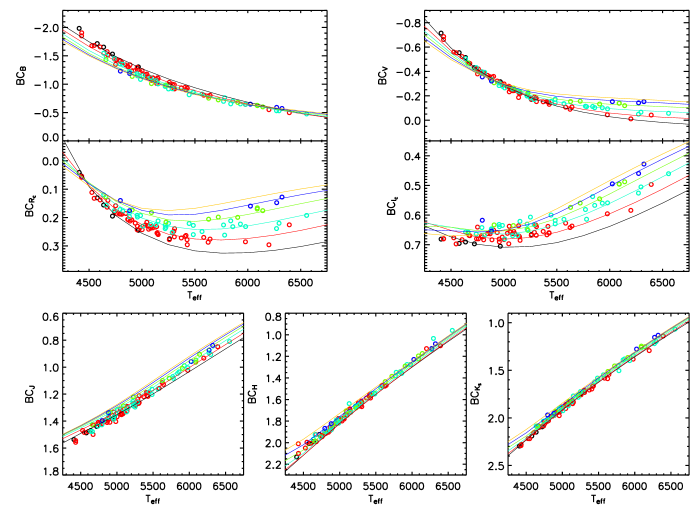
This plot can be regarded as the theoretical counterpart of Figure 2. Again, the agreement between model atmospheres and empirical data is very good and it should be remembered that the model dependence in deducing empirical bolometric correction from our implementation of the IRFM is small (only few 10 %, see Section 4).

A complementary way of deriving stellar integrated fluxes is via photometric indices. The integrated flux of a star, $\mathcal{F}_{Bol}\textrm{(Earth)}$, depends primarily on its apparent brightness (especially in $R_{C}$ and $I_{C}$ bands, see later), which may be measured by its magnitude in different bands. Of lesser importance is its temperature, which is a function of a colour index and metallicity, $\phi(X,\textrm{[Fe/H]})$. Following Blackwell & Petford (1991a), we expect a relation of the form

$$\mathcal{F}_{Bol}\textrm{(Earth)}=10^{-0.4m_{\zeta}}\phi(X,\textrm{[Fe/H]}).$$ (15)

The function $\phi(X,\textrm{[Fe/H]})$ is illustrated in Figure 18, in which the reduced flux in $\zeta$-band, $\mathcal{F}_{Bol}\textrm{(Earth)}\,10^{0.4\,m_{\zeta}}$, is plotted against different colour indices. For the integrated stellar flux we have fitted expressions of the form:

$$\mathcal{F}_{Bol}\textrm{(Earth)}=10^{-0.4m_{\zeta}}\Big{[}b_{0}+b_{1}X+b_{2}X^{2}+b_{3}X^{3}$$

$$\phantom{\mathcal{F}_{Bol}\textrm{(Earth)}=\Big{[}}+b_{4}X\textrm{[Fe/H]}+b_{5}\textrm{[Fe/H]}+b_{6}\textrm{[Fe/H]}^{2}\Big{]}.$$ (16)

We tried different fitting formulae but this form proved the most satisfactory. There are a few fits of this type in the literature (Blackwell & Petford 1991a for a subset of the colours used here, and Alonso et al. 1995 for the infrared). Blackwell et al’s fit has no metallicity dependence because metallicities were not available. Alonso et al’s formula gives fits which are good in the IR but do not reproduce the observed trend in the optical bands. Our fitting formulae work well from optical to IR. As for the temperature-colour fitting, at every iteration points departing more than $3\sigma$ from the mean fit were discarded. The coefficients of the fits, together with the number of stars used, the range of applicability and the standard deviation of the differences between the measured fluxes and the fluxes calculated from the fitting formula are given in Table 10.

Figure 18: Reduced flux in different $\zeta$-bands ($\mathcal{F}_{Bol}\textrm{(Earth)}\,10^{0.4\,m_{\zeta}}$) plotted as function of different colour indices. Squares are for stars with [Fe/H] $\leq-0.5$, crosses for stars with [Fe/H] $>-0.5$.

Table 10: Coefficients and range of applicability of the absolute flux calibrations. All calibrations are valid for the metallicity range $-1.87\leq\textrm{[Fe/H]}\leq 0.34$.

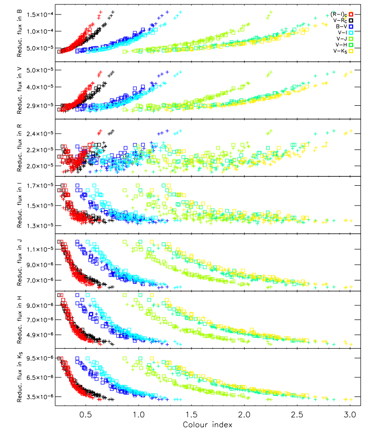
Reduced	Colour	Colour	$b_{0}$	$b_{1}$	$b_{2}$	$b_{3}$	$b_{4}$	$b_{5}$	$b_{6}$	$N$	$\sigma(\%)$
flux		range
$B$	$B-V$	$\left[0.419,1.270\right]$	1.6521	8.6205	$-$13.7586	12.5042	$-$0.7734	$-$0.0644	$-$0.0882	100	1.7
	$V-R_{C}$	$\left[0.249,0.755\right]$	0.4475	19.0419	$-$32.6586	44.0700	$-$0.8436	0.4652	0.1417	98	2.3
	$(R-I)_{C}$	$\left[0.268,0.640\right]$	11.3466	$-$69.2615	184.7907	$-$105.3337	4.8308	$-$1.1543	0.1516	101	3.5
	$V-I_{C}$	$\left[0.517,1.395\right]$	3.9334	$-$4.2082	7.7254	0.7865	0.5466	$-$0.1401	0.1045	99	1.8
	$V-J$	$\left[0.867,2.251\right]$	-0.5405	9.0544	$-$6.6975	2.5713	0.5042	$-$0.2272	0.1393	99	2.5
	$V-H$	$\left[1.016,2.847\right]$	-1.3883	8.9784	$-$5.3419	1.4980	0.5184	$-$0.3228	0.1759	99	2.4
	$V-K_{S}$	$\left[1.124,3.010\right]$	-0.3850	6.4601	$-$3.5378	1.0324	0.4693	$-$0.4049	0.1425	102	2.0
$V$	$B-V$	$\left[0.419,1.270\right]$	2.9901	$-$1.9408	1.6146	0.9227	$-$0.0857	$-$0.3010	$-$0.0800	96	1.5
	$V-R_{C}$	$\left[0.249,0.755\right]$	2.4783	$-$0.6395	2.4817	3.3947	$-$0.0222	$-$0.1769	$-$0.0100	103	1.2
	$(R-I)_{C}$	$\left[0.268,0.640\right]$	6.0078	$-$28.2448	69.7676	$-$44.6415	1.2198	$-$0.5151	0.0052	99	1.7
	$V-I_{C}$	$\left[0.517,1.395\right]$	3.7933	$-$5.2461	6.3043	$-$1.4363	0.1987	$-$0.2959	$-$0.0118	100	0.9
	$V-J$	$\left[0.867,2.251\right]$	2.9726	$-$0.9034	0.3570	0.1879	0.1641	$-$0.3144	0.0062	96	0.9
	$V-H$	$\left[1.016,2.847\right]$	2.5911	$-$0.0458	$-$0.1431	0.1563	0.1532	$-$0.3338	0.0121	99	0.9
	$V-K_{S}$	$\left[1.124,3.010\right]$	3.0690	$-$0.8886	0.3413	0.0497	0.1410	$-$0.3528	0.0024	102	0.9
$R$	$B-V$	$\left[0.419,1.270\right]$	2.6213	$-$2.0936	1.6873	$-$0.1037	$-$0.0267	$-$0.1361	$-$0.0229	100	1.0
	$V-R_{C}$	$\left[0.249,0.755\right]$	2.4703	$-$2.9446	4.5916	$-$1.0001	0.0889	$-$0.1652	$-$0.0075	103	1.2
	$(R-I)_{C}$	$\left[0.268,0.640\right]$	3.7090	$-$12.3326	26.6386	$-$16.4346	0.5423	$-$0.3234	$-$0.0055	101	0.9
	$V-I_{C}$	$\left[0.517,1.395\right]$	2.9332	$-$3.1362	2.9790	$-$0.7098	0.1182	$-$0.2203	$-$0.0090	103	1.0
	$V-J$	$\left[0.867,2.251\right]$	2.9077	$-$1.7416	0.9045	$-$0.1007	0.0983	$-$0.2532	$-$0.0046	95	0.6
	$V-H$	$\left[1.016,2.847\right]$	2.6787	$-$0.9882	0.3538	$-$0.0127	0.0790	$-$0.2506	$-$0.0041	91	0.6
	$V-K_{S}$	$\left[1.124,3.010\right]$	2.8723	$-$1.2499	0.4812	$-$0.0383	0.0689	$-$0.2430	$-$0.0070	93	0.6
$I$	$B-V$	$\left[0.419,1.270\right]$	2.6225	$-$3.6174	3.4760	$-$1.1216	0.0101	$-$0.0438	$-$0.0060	98	1.0
	$V-R_{C}$	$\left[0.249,0.755\right]$	2.7401	$-$7.1587	12.3123	$-$7.0236	0.1591	$-$0.1251	$-$0.0077	100	1.0
	$(R-I)_{C}$	$\left[0.268,0.640\right]$	3.2531	$-$11.0246	21.2495	$-$13.5880	0.4144	$-$0.2412	$-$0.0038	102	1.0
	$V-I_{C}$	$\left[0.517,1.395\right]$	2.9439	$-$4.3412	3.9408	$-$1.1868	0.1287	$-$0.1717	$-$0.0061	103	1.0
	$V-J$	$\left[0.867,2.251\right]$	2.9412	$-$2.6212	1.4468	$-$0.2658	0.0881	$-$0.1967	$-$0.0077	97	1.1
	$V-H$	$\left[1.016,2.847\right]$	2.8196	$-$1.8941	0.8205	$-$0.1187	0.0645	$-$0.1866	$-$0.0077	96	1.1
	$V-K_{S}$	$\left[1.124,3.010\right]$	2.8475	$-$1.8308	0.7520	$-$0.1031	0.0540	$-$0.1688	$-$0.0078	100	1.0
$J$	$B-V$	$\left[0.419,1.270\right]$	2.4518	$-$4.0671	3.2357	$-$0.9315	$-$0.0658	0.1077	0.0185	93	2.2
	$V-R_{C}$	$\left[0.249,0.755\right]$	2.8867	$-$10.0254	15.7145	$-$8.5556	0.0763	$-$0.0217	0.0067	93	2.0
	$(R-I)_{C}$	$\left[0.268,0.640\right]$	3.7432	$-$15.8775	27.7771	$-$16.6189	0.3220	$-$0.1709	0.0065	94	2.5
	$V-I_{C}$	$\left[0.517,1.395\right]$	3.2376	$-$6.2189	5.1663	$-$1.4808	0.0931	$-$0.0901	0.0061	90	2.1
	$V-J$	$\left[0.867,2.251\right]$	2.7711	$-$2.8212	1.3163	$-$0.2179	0.0628	$-$0.1140	0.0022	96	0.9
	$V-H$	$\left[1.144,2.847\right]$	2.8830	$-$2.4146	0.9164	$-$0.1227	0.0382	$-$0.0962	0.0003	91	1.7
	$V-K_{S}$	$\left[1.124,3.010\right]$	2.7876	$-$2.1525	0.7601	$-$0.0949	0.0294	$-$0.0732	0.0039	90	1.5
$H$	$B-V$	$\left[0.419,1.270\right]$	2.3593	$-$4.3075	3.3103	$-$0.9179	$-$0.1030	0.1659	0.0263	97	2.9
	$V-R_{C}$	$\left[0.249,0.755\right]$	2.7616	$-$10.2963	15.6654	$-$8.2985	0.0264	0.0186	0.0097	95	2.8
	$(R-I)_{C}$	$\left[0.268,0.640\right]$	3.5683	$-$15.8279	26.9524	$-$15.7470	0.3107	$-$0.1504	0.0105	95	3.2
	$V-I_{C}$	$\left[0.517,1.395\right]$	3.0862	$-$6.2854	5.0826	$-$1.4230	0.0780	$-$0.0624	0.0083	95	2.8
	$V-J$	$\left[0.867,2.251\right]$	2.6182	$-$2.8623	1.2906	$-$0.2070	0.0518	$-$0.0823	0.0053	99	2.5
	$V-H$	$\left[1.016,2.847\right]$	2.4555	$-$2.0593	0.7245	$-$0.0916	0.0386	$-$0.0839	0.0028	100	1.0
	$V-K_{S}$	$\left[1.124,3.010\right]$	2.5220	$-$2.0243	0.6752	$-$0.0804	0.0246	$-$0.0505	0.0049	97	2.0
$K_{S}$	$B-V$	$\left[0.419,1.270\right]$	2.2158	$-$4.0992	3.1957	$-$0.9165	$-$0.0680	0.1228	0.0208	102	2.8
	$V-R_{C}$	$\left[0.249,0.755\right]$	2.6509	$-$10.0609	15.4526	$-$8.3102	0.0587	$-$0.0096	0.0049	97	2.9
	$(R-I)_{C}$	$\left[0.268,0.640\right]$	3.2130	$-$13.9314	23.1287	$-$13.2435	0.3450	$-$0.1801	0.0049	100	2.9
	$V-I_{C}$	$\left[0.517,1.395\right]$	2.8573	$-$5.7901	4.6467	$-$1.3010	0.0958	$-$0.0924	0.0028	103	2.7
	$V-J$	$\left[0.867,2.251\right]$	2.5152	$-$2.8220	1.2970	$-$0.2136	0.0645	$-$0.1172	$-$0.0001	100	2.6
	$V-H$	$\left[1.016,2.847\right]$	2.4184	$-$2.1148	0.7671	$-$0.1005	0.0453	$-$0.1096	$-$0.0014	95	2.2
	$V-K_{S}$	$\left[1.124,3.010\right]$	2.4209	$-$1.9857	0.6720	$-$0.0819	0.0323	$-$0.0795	0.0005	102	1.0

$N$ is the number of stars used for the fit after the $3\sigma$ clipping and $\sigma(\%)$ the standard deviation of the percentage differences between the measured fluxes and the fluxes calculated from the fitting formula. The coefficients of the calibrations $b_{i}$ are given in units of $10^{-5}$ erg cm^-2 s^-1.

The scatter in Figure 18 of the reduced flux in $R_{C}$ and $I_{C}$ bands is only apparently large, due to the small range (in vertical scale) covered by the reduced fluxes in these two colours (compare also with Figure 17). For the sake of the proposed calibration, the small range covered by the reduced flux in these two bands allows for a very accurate (at 1% level or below) calibration. Interestingly, for these two bands tight relations also exist between bolometric fluxes and magnitudes, as seen in Figure 19.

Figure 19: Left panel: relation between apparent magnitudes in $\zeta=R_{C}$ (circles) and $\zeta=I_{C}$ (crosses) band and bolometric fluxes on the Earth (in erg cm^-2 s^-1). Right panel: relation between absolute magnitudes in the same $R_{C}$ and $I_{C}$ bands and absolute bolometric magnitudes. The fit is in the form $\gamma=A+B\zeta$, $\sigma(\%)$ is the standard deviation of the percentage differences between the measured values and those calculated from the fit and $N$ is the number of stars employed for the fitting after the $3\sigma$ clipping.

8 The Angular-diameter-colour relation

Limb-darkened angular diameters can then be readily obtained via equation (5) from the temperature and bolometric flux calibrations given in Section 4 and 7. In particular, when using J magnitudes with various colour indices, we have found very tight and simple relations, as can be appreciated from Figure 20. Analogous relations in other bands are significantly less tight.

Figure 20: Empirical angular diameter-colour relations for our sample of stars.

We have fitted relations of the form

$$\theta=c_{0}+c_{1}\sqrt{\phi(m_{J},X)}$$ (17)

where

$$\phi(m_{J},X)=10^{-0.4m_{J}}X$$ (18)

for a given colour index $X$.

Table 11: Coefficients and range of applicability of the angular diameter calibrations.

Colour	Colour range	$c_{0}$	$c_{1}$	$N$	$\sigma(\%)$	$\sigma$(mas)
$B-V$	[0.419, 1.270]	0.00647	6.18657	102	3.4	0.008
$V-R_{C}$	[0.249, 0.755]	0.00340	8.26244	103	2.7	0.008
$(R-I)_{C}$	[0.268, 0.640]	$-$0.00385	8.97758	103	2.0	0.006
$V-I_{C}$	[0.517, 1.395]	$-$0.00045	6.09487	102	1.6	0.005
$V-J$	[0.867, 2.251]	0.00057	4.63147	103	1.6	0.005
$V-H$	[1.016, 2.847]	$-$0.00022	4.13607	102	1.3	0.004
$V-K_{S}$	[1.124, 3.010]	0.00098	4.01335	103	1.2	0.003
$J-K_{S}$	[0.257, 0.759]	0.00300	7.96076	100	2.8	0.007

$N$ is the number of stars used for the fit after the $3\sigma$ clipping. $\sigma(\%)$ is the standard deviation of the percentage differences between the angular diameters obtained via IRFM and those calculated from the fitting formula. $\sigma$(mas) is the standard deviation in terms of mas.

As can be appreciated from Table 11, these relations show remarkably small scatter (at the few percent level). In particular, the upper range covered in angular diameters can be used to build a network of small calibrators for future long-baseline interferometric measurements from readily available broadband photometry.

The calibration in $J-K_{S}$ colour is particularly appealing, since in this photometric index the effect of interstellar extinction is negligible.

The given angular diameter scale can be tested with the G dwarf HD 209458 A for which the linear radius has been calculated from planetary transit (Brown et al. 2001). We have taken $V$ magnitude from Hipparcos and $J$, $H$ and $K_{S}$ from 2MASS. Our predicted value of $\theta=0.227\pm 0.003$ mas is in excellent agreement with that of $\theta=0.228\pm 0.004$ mas obtained by Kervella et al. (2004) using surface brightness relations calibrated by interferometry. The difference between the two values is only 0.4% and therefore well below the possible $\sim 3\%$ offset previously discussed. Unfortunately, both this comparison and those in Section 5 and 6.1 have their own limitations since they are indirect, or sensitive to photometric uncertainties (for this star, Kervella has to convert the 2MASS $K_{S}$ magnitude into the Johnson system used to fit his relations). When our angular size is translated into linear radius via Hipparcos parallaxes we obtain $R=1.150\,\pm\,0.056\,R_{\odot}$ slightly smaller than that of Kervella et al. (2004) but in better agreement with the direct estimate of $R=1.146\,\pm\,0.050\,R_{\odot}$ obtained by Brown et al. (2001) via $HST$ time-series photometry (although all determinations agree well within the error budget). Unfortunately, in this case the uncertainty in parallax dominates the bulk of the $\sim 5\%$ uncertainty on the radius.

Table 12: Predicted angular diameter for HD 209458 A.

$V$	$J$	$H$	$K_{S}$	$\theta_{V-J}$	$\theta_{V-H}$	$\theta_{V-K_{S}}$	$\theta$
7.65	6.591	6.366	6.308	0.230	0.225	0.224	0.227
$\pm 0.01$	$\pm 0.020$	$\pm 0.038$	$\pm 0.026$				$\pm 0.003$

$\theta_{\xi-\zeta}$ are the angular diameters obtained when $(V-J)$, $(V-H)$ and $(V-K_{S})$ colour indices are used. Since the accuracy of the calibration in these bands is very similar (see Table 11), the final angular diameter is the average of the three values weighted by the photometric errors.

9 Conclusions

We have used the Infrared Flux Method to deduce fundamental stellar parameters of effective temperature, bolometric magnitude and angular diameter for a sample of 104 G and K dwarfs. This semi-direct method is mostly based on empirical data obtained from our own observations or carefully selected from the literature in order to achieve the highest accuracy feasible. Our stars all have excellent $BV(RI)_{C}JHK_{S}$ photometry, excellent parallaxes and good metallicities.

Most of the bolometric flux of our stars is seen in the optical and infrared bands covered $BV(RI)_{C}JHK_{S}$. For the remaining 15 to 30% of the flux lying outside these bands, model atmospheres have been used. Good to very good agreement is found for the colours of the stars and the synthetically derived colours of a number of sets of model atmospheres in the literature (ATLAS9, MARCS, BaSel 3.1).

The zero-points of our temperature, luminosity and angular diameter scales (Sections 4, 7 and 8) depend only on our adopted absolute calibration of Vega. The advantages and disadvantages of our use of Vega are discussed in Appendix A. The main advantage is that Vega’s absolute calibration has been extensively studied over a wide wavelength range via satellite measurements. This allows us to put firm constraints on the systematic uncertainties. A likely disadvantage is that Vega is known to be pole-on and a fast rotator which prevents the use of a unique Vega model atmosphere in fitting the observations.

Our calibration of effective temperature is found to be some 100 K hotter than similar determinations in the literature, while it is also found to be in close agreement with effective temperature scales based on spectroscopic methods. To reduce our temperature scale by 100 K, the required changes to Vega’s 2MASS zero-points and/or absolute calibration are significantly larger than the known uncertainties in these quantities. Neither can the model atmospheres be blamed, because we find such good agreement between the model atmosphere colours and the empirical data. We worked hard to impute inconsistency to one or other of the scales, but were unable to resolve the issue beyond any reasonable doubt. Our angular diameters are smaller by about 3% with respect to other indirect determinations, but they seem more in line with the predictions of asteroseismology and 3D model atmospheres. We conclude that temperatures, luminosities and angular diameters calibrations for lower main sequence G and K dwarfs retain systematics of the order of a few percent.

The high quality and homogeneity of the data produce very tight empirical colour–metallicity–temperature and angular diameter–colour calibrations. In particular, the relation between angular diameters and magnitudes in the $J$ band is remarkable and it indicates an high sensitivity of this band to angular diameters. Since many lower main sequence stars are known to host planets, our relations can be used to accurately determine the physical properties of the parent star thus allowing to effectively break the degeneracy between the properties of the stars and that of the planets when extremely high precision data are unavailable (e.g. Bakos et al. 2005, Sato et al. 2005).

Future interferometric measurements of angular diameters would go a long way to addressing the uncertainties we have shown as well as to test our findings. In particular, the shape of the visibility function in the second lobe would directly probe limb-darkening corrections (e.g. Bigot et al. 2006) for our stars. Likewise, tying the absolute calibration and the observed colours to a solar twin would probably reduce many of these uncertainties. At present good candidate solar twins are HD 146233 (Porto de Mello & da Silva) and HD 98618 (Meléndez et al. 2006). Accurate interferometric measurements together with high precision photometry for a set of nearby solar-like stars would permit to set the absolute calibration via solar analogs directly (e.g. Campins et al. 1985). Besides, extremely high precision multiple bandpass studies of transiting extra-solar planets would provide direct angular diameter estimates for our stars, and will further test our temperature scale.

Appendix A Broad-band synthetic photometry and absolute calibration

The choice of the zero-points is of critical importance to set synthetic and real photometry on the same scale. Historically, the zero-points of the $UBV$ system were defined “in terms of unreddened main-sequence stars of class A0 …with an accuracy sufficient to permit the placement of the zero-point to about 0.01 mag” (Johnson & Morgan, 1953). The pioneering work of Johnson was continued and extended to other bands by Johnson himself over the years; in the southern hemisphere Cousins (1976, 1978, 1980) and astronomers at the South African Astronomical Observatory (SAAO) refined its accuracy and colours range (Menzies et al. 1989; Kilkenny et al. 1998). Similar work was carried out in the northern hemisphere by Landolt (1992) at the CTIO. Subtle differences exist between different works (see Bessell 2005 for a review) and especially between the SAAO and the CTIO system (Bessell 1995). Nevertheless, the $BV(RI)_{C}$ system is nowadays a well defined one whose main characteristics and bandpasses are given in Bessell (1990b).

The basic equation of synthetic photometry in a given band $\zeta$ reads as follows (e.g. Girardi et al. 2002):

$$m_{\zeta}=-2.5\log\left[\left(\frac{R}{d}\right)^{2}\frac{\int_{\lambda_{\zeta_{i}}}^{\lambda_{\zeta_{f}}}F(\lambda)T_{\zeta}(\lambda)\textrm{d}\lambda}{\int_{\lambda_{\zeta_{i}}}^{\lambda_{\zeta_{f}}}T_{\zeta}(\lambda)\textrm{d}\lambda}\right]+\textrm{ZP}_{\zeta}$$ (19)

where $F(\lambda)$ is the flux of the synthetic spectrum (given in erg cm^-2 s^-1 Å^-1), $T_{\zeta}(\lambda)$ the transmission curve of the filter comprised in the interval $(\lambda_{\zeta_{i}},\lambda_{\zeta_{f}})$ and $\textrm{ZP}_{\zeta}$ the zero-point for the $\zeta$ band. The ratio between the radius $R$ of the star and its distance $d$ from us is known as the dilution factor and relates to the angular diameter $\theta$ (corrected for limb darkening) via:

$$\theta=2\,\frac{R}{d}$$ (20)

where $\theta$ is in radians. We also note that when all quantities in the logarithmic term of eq. (19) are known that gives the absolute calibration in $\zeta$-band (see Table 14) for a star with spectrum $F(\lambda)$.

While the zero-points of observational photometry are defined on an ensemble of well measured stars, for synthetic photometry a common choice is to set the zero-points using a reference star for which all the physical quantities in eq. (19), i.e. the spectrum $F(\lambda)$ (usually synthetic), the dilution factor and the observed apparent magnitudes or colour indices are known in detail.

This star is usually Vega, for which we have used the magnitudes and colours given in Table 13. The optical colours are from Bessell (1990a), whereas for the 2MASS system they come from Cohen et al. (2003). The latter were determined post-facto, comparing the observed 2MASS magnitudes of 33 stars with the values predicted from the absolutely calibrated templates built by Cohen et al. (2003) within the “Cohen-Walker-Witteborn” (1992a) framework.

Table 13: Observed magnitudes for Vega.

$B$	$V$	$R_{C}$	$I_{C}$	$J$	$H$	$K_{S}$	Ref.
0.02	0.03	0.039	0.035				Bessell 1990a
				$-$0.001	+0.019	$-$0.017	Cohen et al. 2003

In principle we could adopt a unique spectrum for Vega and use it to compute zero-points from $B$ to $K_{S}$; in this way the dependence on the absolute calibration would cancel out when computing colour indices, since all colours scale in the same way with the adopted absolute calibration. In practice we use a slightly different approach using two models, one for the absolute calibration in the optical and one in the infrared – each consistent with the corresponding data source.

The 2MASS magnitudes for Vega are deduced in the absolutely calibrated system that is ultimately defined on the Kurucz spectra for Vega and Sirius used by Cohen et al. (1992b). Therefore, for the $JHK_{S}$ bands we have adopted the zero-magnitude fluxes provided by Cohen et al. (2003). The zero-magnitude fluxes proposed by Cohen for Vega and eight of the primary and secondary stars in the calibration network of “Cohen-Walker-Witteborn” has been recently confirmed in the $4$–$24\,\mu m$ range by the Midcourse Space Experiment (MSX) flux calibration (Price et al. 2004) to be accurate around 1% and thus well within the global error of 1.46% quoted by Cohen, even though it seems that the fluxes of Cohen in the infrared should be brightened by 1%. Also, Tokunaga & Vacca (2005) have shown the Vega absolute calibration of Cohen et al. (1992b) and the model–independent measurements of Megessier (1995) to be identical within the uncertainties in the range $\sim$ 1–4 $\mu m$.

For the absolute calibration in the optical bands we have adopted a Kurucz (2003) synthetic spectrum for Vega with $T_{\mathrm{e}ff}=9550$ K, $\log(g)=3.95$, [M/H] = $-$0.5 and microturbulent velocity $\xi=2\,{\rm km}\;{\rm s}^{-1}$. The resolving power used has been 500. This model has recently shown excellent agreement with the Space Telescope Imaging Spectrograph (STIS) flux distribution over the range $0.17$–$1.01\,\mu m$ (Bohlin & Gilliland 2004). In particular, in the regions of the Balmer and Paschen lines the STIS equivalent widths differ from the pioneering work of Hayes (1985) (and used by Colina et al. 1996 to assemble a composite spectrum of Vega) but do agree with the predictions of the Kurucz model.

Once the synthetic spectrum of Vega in the optical bands is chosen, we need to scale it in order to match the absolute flux of Vega as measured on the Earth at a certain fixed wavelength ($\lambda$). The monochromatic flux given by the model $F_{\textrm{\scriptsize{model}}}(\lambda)$ is simply related to the same monochromatic flux as measured on the Earth $F_{\textrm{\scriptsize{Earth}}}(\lambda)$ by

$$F_{\textrm{\scriptsize{Earth}}}(\lambda)=\left(\frac{R}{d}\right)^{2}F_{\textrm{\scriptsize{model}}}(\lambda)$$ (21)

where the dilution factor $(R/d)^{2}$ is the ratio between the radius of Vega and its distance. In principle the dilution factor can be deduced from direct measures of Vega’s angular diameter. In practice, since such measures are more uncertain than direct measures of the flux, we proceed the other way around. Taking the flux value at 5556 Å from Megessier (1995) $F_{\textrm{\scriptsize{Earth}}}(5556\,\textrm{\AA})=3.46\times 10^{-9}$ erg cm^-2 s^-1 Å^-1 and at the same wavelength from the Kurucz (2003) Vega model $F_{\textrm{\scriptsize{model}}}(5556\,\textrm{\AA})=5.5015572\times 10^{7}$ erg cm^-2 s^-1 Å^-1 we obtain $(R/d)^{2}=6.2891286\times 10^{-17}$. This value implies and angular diameter of 3.272 mas for Vega, which compares very well with the interferometric angular diameter measurements of $3.24\pm 0.07$ mas (Code et al. 1976), $3.28\pm 0.06$ mas (Ciardi et al. 2001) and $3.225\pm 0.032$ (Mozurkewich et al. 2003).

We chose to use the Megessier flux in accordance with the absolute scale adopted for the STIS (Bohlin & Gilliland 2004) rather than the value of $3.44\times 10^{-9}$ erg cm^-2 s^-1 Å^-1 $\pm 1.45$% found in Hayes (1985) and used by Cohen to tie his absolute calibration in the infrared. A thorough discussion of the differences in the infrared is given by Bohlin & Gilliland (2004); here we just mention that this choice together with the Kurucz (2003) model in the infrared would give a flux density of Vega about 2% lower than in Cohen, thus worsening the agreement with MSX. On the other hand, the STIS absolute calibration in the optical is expected to be better than 2% (Bohlin 2000). In this range, the increase of $0.6$% relative to Hayes translates in absolute fluxes that are higher by the same factor and in differences for the $BV(RI)_{C}$ zero-points of 0.006 mag.

Table 14: Absolute calibration and effective wavelength of the ground-based optical-IR photometry of Vega used in this work. Quantities tabulated correspond to the definition of the zero magnitude in each filter.

Band	$\lambda_{\mathrm{e}ff}$	Monochromatic Absolute Flux	Uncertainty	Ref.
	Å	erg cm-2 s-1Å-1	erg cm-2 s-1Å-1
$B$	4362	6.310E-9	6.310E-11	This paper
$V$	5446	3.607E-9	3.607E-11	This paper
$R_{C}$	6413	2.153E-9	2.153E-11	This paper
$I_{C}$	7978	1.119E-9	1.119E-11	This paper
$J$	12285	3.129E-10	5.464E-12	Cohen et al. (2003)
$H$	16385	1.133E-10	2.212E-12	Cohen et al. (2003)
$K_{S}$	21521	4.283E-11	8.053E-13	Cohen et al. (2003)

The effective wavelengths associated to each filter are computed in accordance with Appendix B. The error in $BV(RI)_{C}$ bands are computed assuming an arbitrary uncertainty of 1% to the absolute flux. Lacking the actual uncertainties in the measurement of the filters’ transmission curve, the adopted uncertainty is consistent with a wavelength–independent filter uncertainty in addition to the 0.7% absolute uncertainty at 5556 Å from Megessier (1995).

Recent work by Gulliver et al. (1994), Peterson et al. (2004, 2006) and Aufdenberg et al. (2006) indicate that Vega is pole-on and fast rotator. Thus standard model atmospheres are not appropriate for Vega, as discussed by Bohlin & Gilliland (2004). Nonetheless STIS in the optical and MSX in the infrared have confirmed the adopted absolute calibrations to be accurate at the percent level. It is interesting to note that Peterson et al. (2006) give an estimate of the shift in Vega’s zero-points as a consequence of the higher infrared flux due to its rapidly rotating nature. Though only indicative, as the authors say, the shifts for their latest non-rotating synthetic spectrum in the infrared amount to $0.05-0.07$ mag. The net effect of such shifts would be to reduce the temperatures recovered via IRFM. Considering that in the infrared we are adopting the absolute calibration given by Cohen (already some $\sim 2\%$ brighter as compared to the latest Kurucz model) this reduces the size of the required shifts to about $0.02-0.04$ mag. The agreement within 1% with MSX would however require a shift of only $0.01$ mag. Since the proposed shifts are only indicative and the measurements confirm the adopted calibration within the errors, we adopt the pragmatic choice of using the model that at any given range better agrees with the data. It is evident from the above discussion that there is no consistent published atmospheric model for Vega at both visible and infrared wavelengths and this justifies our adoption of the Kurucz (2003) or Cohen models at different wavelengths. Likewise, the use of composite model atmospheres for Vega is also advocated from Peterson et al. (2006). For synthetic photometry the use of composite spectra is often avoided on the reason that fixing the zero-points, possible physical deficiencies in the synthetic spectrum of Vega are likely to be present in the synthetic library and therefore they would cancel out (e.g. Girardi et al. 2002). In our case the situation is not so clear, since synthetic spectra give now excellent comparison with the real ones and the deficiencies for Vega are likely to be due to the particular nature of this star.

Sirius is often used as an additional fundamental colour standard (e.g. Bessell, Castelli & Plez 1998), allowing one to control the possible problems of putative variability and an IR excess for Vega. First seen by Aumann (1984) beyond 12 $\mu m$, Vega’s variability at shorter wavelengths has long been a matter of discussion (see e.g. Bessell, Castelli & Plez 1998; Ciardi et al. 2001), though the rapidly rotating model could actually resolve the controversy (Peterson at al. 2006). The most recent data from MSX (Price et al. 2004) and SPITZER (Su et al. 2005) support models where Vega’s infrared excess and variability is due to a cold dust disk. The IR excess increase steadily longward of $12\,\mu m$ whereas at $4\,\mu m$ the differences between model atmosphere and measurements are entirely consistent within the uncertainties and therefore should not affect the optical and near-infrared region (0.36 – 2.4 $\mu m$) we are working with. For the sake of completeness we have tested the differences in the derived $BV(RI)_{C}$ zero-points when including Sirius in the calibration. Adopting the latest Kurucz model available for it and the colours from Bessell (1990a), the differences in the derived zero-points between the use of Vega only or Vega plus Sirius range from 0.008 mag in $B-V$ to 0.002 mag in $(R-I)_{C}$. Such differences are below the uncertainties in magnitude and colours. In addition, since absolute calibration and magnitudes for Sirius in the 2MASS system are not available, we have decided to adopt only Vega as our standard star. This also makes clearer the comparison between synthetic colours and the IRFM that strongly depends on the Vega absolute calibration.

The transmission curves used come from Bessell (1990b) for the Johnson-Cousins $BV(RI)_{C}$ system and from Cohen et al. (2003) for the 2MASS $JHK_{S}$ system.

The 2MASS transmission curves carefully incorporate the effect of the optical system, the detector quantum efficiency and the site-specific atmospheric transmissions. The effect of the telescope optics on the estimated $BV(RI)_{C}$ passband are not counted, but in the $V$ band this has been proved to cause uncertainty below few millimag (Colina & Bohlin, 1994), and thus smaller than any possible observational error we are going to compare with.

We note that all our photometry is reduced to zero airmass and when we refer to measurements on the Earth, we always mean at the top of the Earth’s atmosphere.

Appendix B Characteristic Parameters of a Photometric System

In the present work we have reduced broadband (heterochromatic) measurement in a band $\zeta$ to a monochromatic flux ($\mathcal{F_{\zeta}}$) by means of the following relation:

$$\mathcal{F_{\zeta}}=\frac{\int_{\lambda_{\zeta_{i}}}^{\lambda_{\zeta_{f}}}F(\lambda)T_{\zeta}(\lambda)\textrm{d}\lambda}{\int_{\lambda_{\zeta_{i}}}^{\lambda_{\zeta_{f}}}T_{\zeta}(\lambda)\textrm{d}\lambda},$$ (22)

where the integration is done in the interval $\lambda_{\zeta_{i}},\lambda_{\zeta_{f}}$ that comprise a given passband $T_{\zeta}(\lambda)$. We remark that the above formulation is suited for both energy integration in the optical and photo-counting in the IR, provided that we are dealing with the Bessell (1990b) and Cohen et al. (2003) transmission curves (see Appendix A).

Assuming that the function $F(\lambda)$ is continuous and that $T_{\zeta}(\lambda)$ does not change sign in the interval $\lambda_{\zeta_{i}},\lambda_{\zeta_{f}}$, the generalization of the mean value theorem states that there is at least one value of $\lambda$ in the interval $\lambda_{\zeta_{i}},\lambda_{\zeta_{f}}$ such that

$$F(\lambda_{i})\int_{\lambda_{\zeta_{i}}}^{\lambda_{\zeta_{f}}}T_{\zeta}(\lambda)\textrm{d}\lambda=\int_{\lambda_{\zeta_{i}}}^{\lambda_{\zeta_{f}}}F(\lambda)T_{\zeta}(\lambda)\textrm{d}\lambda.$$ (23)

Rearranging this, we obtain

$$\mathcal{F}_{\zeta}=F(\lambda_{i})=\frac{\int_{\lambda_{\zeta_{i}}}^{\lambda_{\zeta_{f}}}F(\lambda)T_{\zeta}(\lambda)\textrm{d}\lambda}{\int_{\lambda_{\zeta_{i}}}^{\lambda_{\zeta_{f}}}T_{\zeta}(\lambda)\textrm{d}\lambda},$$ (24)

where $\lambda_{i}$ is the isophotal wavelength. The isophotal wavelength is thus the wavelength which must be given to the monochromatic quantity $F(\lambda_{i})$ obtained from a heterochromatic measurement.

Stellar spectra do not necessarily satisfy the requirements of the mean value theorem for integration, as they exhibit discontinuities. Although the mean value of the intrinsic flux is well-defined (and we have extensively used it), the determination of the isophotal wavelength becomes problematic because spectra contain absorption lines and hence the definition can yield multiple solutions.

Several authors avoid using the isophotal wavelength and introduce the effective wavelength defined by the following expression

$$\lambda_{\mathrm{e}ff}=\frac{\int_{\lambda_{\zeta_{i}}}^{\lambda_{\zeta_{f}}}\lambda F(\lambda)T_{\zeta}(\lambda)\textrm{d}\lambda}{\int_{\lambda_{\zeta_{i}}}^{\lambda_{\zeta_{f}}}F(\lambda)T_{\zeta}(\lambda)\textrm{d}\lambda}.$$ (25)

This is the mean wavelength of the passband as weighted by the energy distribution of the source over the band. The effective wavelength is thus an approximation for $\lambda_{i}$, however since the monochromatic magnitude at the effective wavelength is almost identical to that at the isophotal wavelength (Golay 1974), we have used the effective wavelength through all our work.

We have verified that the detailed choice of the wavelength associated to a monochromatic flux is not crucial for the derived correction of the $\mathcal{C}$ factor (eq. 3).

When dealing with photometric data, a way to obtain monochromatic flux from heterochromatic measurements is provided by the $q$ factor. Ideally the $q$-factor (eq. 8) should be determined from spectroscopic data but in practice we rely on a grid of models. Since the absolute monochromatic flux for a given band is determined as described in Appendix A, the definition of the $q$-factor for a star with spectra $F(\lambda)$ is now:

$$q(\lambda_{\textrm{\tiny{IR}}})=\frac{\int_{\lambda_{i}}^{\lambda_{f}}T_{\textrm{\tiny{IR}}}(\lambda)\textrm{d}\lambda}{\frac{1}{F(\lambda_{\textrm{\tiny{IR}}})}\int_{\lambda_{i}}^{\lambda_{f}}F(\lambda)T_{\textrm{\tiny{IR}}}\textrm{d}\lambda}$$ (26)

This definition slightly differs from that given by Alonso et al. (1994, 1996b) to reflect the different absolute calibration we have adopted (i.e. argument of the logarithm in equation 19). However, the different definition of the $q$ factor has only minor effects on the recovered stellar parameters. Using the definition of Alonso et al. (1996b) would go in the direction of making temperatures hotter by 20 to 30 K on average, the difference increasing with increasing temperature. On average also luminosities would be brighter by 0.14% and angular diameters smaller by 0.9%.

References

- Allende-Prieto (2002) Allende Prieto C., Asplund M., López R.J.G., Lambert D.L., 2002, ApJ, 567, 544
- Allende-Prieto (2004) Allende Prieto C., Barklem P.S., Lambert D.L., Cunha K., 2004, A&A, 420, 183
- Aller (1963) Aller L.H., 1963, The Atmosphere of the Sun and Stars, N.Y. Ronald Press
- Alonso (1994) Alonso A., Arribas S., Martínez-Roger C., 1994, A&A, 282, 684
- Alonso (1995) Alonso A., Arribas S., Martínez-Roger C., 1995, A&A, 297, 197
- Alonso (1996a) Alonso A., Arribas S., Martínez-Roger C., 1996a, A&A, 313, 873
- Alonso (1996b) Alonso A., Arribas S., Martínez-Roger C., 1996b, A&A, 117, 227
- Anders (1989) Anders E., Grevesse N., 1989, Geochim. Cosmochim. Acta, 53, 197
- Asplund (2003) Asplund M., 2003, in IAU Joint Discussion, 15, Elemental Abundances in Old Stars and Damped Lyman- Systems, p.8 (astro-ph/0310445)
- Aufdenberg (2006) Aufdenberg J.P. et al., 2006, preprint(astro-ph/0603327)
- Aumann (1984) Aumann H.H. et al., 1984, ApJ, 278, 23
- Bahcall (2005) Bahcall J.N., Serenelli A.M., Basu S., 2005, preprint(astro-ph/0511337)
- Bai (2004) Bai G.S., Zhao G., Chen Y.Q., Shi J.R., Klochkova V.G., Panchuk V.E., Qiu H.M., Zhang H.W., 2004, A&A, 425, 671
- Bakos (2006) Bakos G.A., et al., 2006, preprint(astro-ph/0603291)
- Beirão (2005) Beirão P., Santos N.C., Israelian G., Mayor M., 2005, A&A, 438, 251
- Bessell (1979) Bessell M.S., 1979, PASP, 91, 589
- Bessell (1990a) Bessell M.S., 1990a, A&AS, 83, 357
- Bessell (1990b) Bessell M.S., 1990b, PASP, 102, 1181
- Bessell (1995) Bessell M.S., 1995, PASP, 107, 672
- Bessell (2005) Bessell M.S., 2005, ARA&A, 43, 293
- Bessell (1984) Bessell M.S., Wood P.R., 1984, PASP, 96, 247
- Bessell (1998) Bessell M.S., Castelli F., Plez B., 1998, A&A, 333, 231
- Bell (1989) Bell R.A., Gustafsson B., 1989, MNRAS, 236, 653
- Bigot (2006) Bigot L., Kervella P., Thévenin F., Ségransan D., 2006, A&A, 446, 635
- Blackwell (1977) Blackwell D.E., Shallis M.J., 1977, MNRAS, 180, 177
- Blackwell (1991a) Blackwell D.E., Petford A.D., 1991a, A&A, 250, 459
- Blackwell (1994) Blackwell D.E., Lynas-Gray A.E., 1994, A&A, 282, 899
- Blackwell (1998) Blackwell D.E., Lynas-Gray A.E., 1998, A&A, 129, 505
- Blackwell (1979) Blackwell D.E., Shallis M.J., Selby M.J., 1979, MNRAS, 188, 847
- Blackwell (1980) Blackwell D.E., Petford A.D., Shallis M.J., 1980, A&A, 82, 249
- Blackwell (1991b) Blackwell D.E., Lynas-Gray A.E., Petford A.D., 1991b, A&A, 245, 567
- Blackwell (1990) Blackwell D.E., Petford A.D., Arribas S., Haddock D.J., Selby M.J., 1990, A&A, 232, 396
- Bohlin (2000) Bohlin R.C., 2000, AJ, 120, 437
- Bohlin (2004) Bohlin R.C., Gilliland R.L., 2004, AJ, 127, 3508
- Bohlin (2001) Bohlin R.C., Dickinson M.E., Calzetti D., 2001, AJ, 122, 2118
- Brewer (2006) Brewer M-M., Carney B.W., 2006, AJ, 131, 431
- Brown (1997) Brown A.G.A., Arenou F., van Leeuwen F., Lindegren L., Luri X., 1997, Hipparcos - Venice 1997 Proc., ESA SP-402. ESA Publications Division, Noordwijk, p.63
- Brown (2001) Brown T.M., Charbonneau D., Gilliland R.L., Noyes R.W., Burrows A., 2001, ApJ, 552, 699
- Campins (1985) Campins H., Rieke G.H., Lebofsky M.J., 1985, AJ, 90, 896
- Cardelli (1989) Cardelli J.A., Clayton G.C., Mathis J.S., 1989, ApJ, 345, 245
- Castelli (2003) Castelli F., Kurucz R.L., 2003, in Piskunov N., Weiss W.W., Gray D.F., eds, Proc. IAU Symp. 210, Modelling of Stellar Atmospheres. Astron. Soc. Pac., p.A20 (astro-ph/0405087)
- Castro (1997) Castro S., Rich R.M., Grenon M., Barbuy B., McCarthy J.K., 1997, AJ, 114, 376
- Cayrel (1996) Cayrel de Strobel G., 1996, A&ARv, 7, 243
- Ciardi (2001) Ciardi D.R., van Belle G.T., Akeson R.L., Thompson R.R., Lada E.A., Howell S.B., 2001, ApJ, 559, 1147
- Clementini (1999) Clementini G., Gratton R.G., Carretta E., Sneden C., 1999, MNRAS, 302, 22
- Code (1976) Code A.D., Bless R.C., Davis J., Brown R.H., 1976, ApJ, 203, 417
- Cohen (1992a) Cohen M., Walker R.G., Witteborn F.C., 1992a, AJ, 104, 2030
- Cohen (1992b) Cohen M., Walker R.G., Barlow M.J., Deacon J.R., 1992b, AJ, 104, 1650
- Cohen (1996) Cohen M., Witteborn F.C., Carbon D.F., Davies J.K., Wooden D.H., Bregman J.D., 1996, AJ, 112, 2274
- Cohen (1999) Cohen M., Walker R.G., Carter B., Hammersley P., Kidger M., Noguchi K., 1999, AJ, 117, 1864
- Cohen (2003) Cohen M., Wheaton Wm. A., Megeath S.T., 2003, AJ, 126, 1090
- Colina (1994) Colina L., Bohlin R.C., 1994, AJ, 108, 1931
- Colina (1997) Colina L., Bohlin R., 1997, AJ, 113, 1138
- Colina (1996) Colina L., Bohlin R.C., Castelli F., 1996, AJ, 112, 307
- Cousins (1976) Cousins A.W.J., 1976, Mem. R. Astron. Soc., 81, 25
- Cousins (1978) Cousins A.W.J., 1978, Mon. Notes Astron. Soc. S. Afr., 37, 8
- Cousins (1980) Cousins A.W.J., 1980, SAAO Circ., 1, 166
- crawford (1975) Crawford, 1975, PASP, 87, 481
- diBenedetto (1998) Di Benedetto G.P., 1998, A&A, 339, 858
- diBenedetto (1987) Di Benedetto G.P., Rabbia Y., 1987, A&A, 188, 114
- Dickinson (2002) Dickinson M., Sosey M., Rieke M., Bohlin R.C., Calzetti D., 2002, in Arribas S., Koekemoer A., Whitmore B., eds., The 2002 HST Calibration Workshop, STScI Baltimore, p.231
- Favata (1997) Favata F., Micela G., Sciortino S., 1997, A&A, 323, 809
- Fremaux (2006) Frémaux J., Kupka F., Boisson C., Joly M., Tsymbal V., 2006, A&A, 449, 109
- Fuhrmann (1993) Fuhrmann K., Axer M., Gehren T., 1993, A&A, 271, 451
- Fuhrmann (1994) Fuhrmann K., Axer M., Gehren T., 1994, A&A, 285, 585
- Fulbright (2000) Fulbright J.P., 2000, AJ, 120, 1841
- Girardi (2002) Girardi L., Bertelli G., Bressan A., Chiosi C., Groenewegen M.A.T., Marigo P., Salasnich B., Weiss A., 2002, A&A, 391, 195
- Golay (1974) Golay M., 1974, Introduction to Astronomical Photometry, (Dordrecht: Reidel)
- Gratton (2003) Gratton R.G., Carretta E., Claudi R., Lucatello S., Barbieri M., 2003, A&A, 404, 187
- Gray (1989) Gray D.F., 1989, ApJ, 347, 1021
- Gray (1994) Gray D.F., 1994, PASP, 106, 1248
- Gray (1991) Gray D.F., Johanson H.L., 1991, PASP, 103, 439
- Gray (2003) Gray R.O., Corbally C.J., Garrison R.F., McFadden M.T., Robinson P.E., 2003, AJ, 126, 2048
- Grevesse (1998) Grevesse N., Sauval A.J., 1998, Space Sci. Rev., 85, 161
- Grupp (2004a) Grupp F., 2004a, A&A, 426, 309
- Grupp (2004b) Grupp F., 2004b, A&A, 420, 289
- Gulliver (1994) Gulliver A.F., Hill G., Adelman S.J., 1994, ApJ, 429, 81
- Gustafsson (1975) Gustafsson B., Bell R.A., Eriksson K., Nordlund A., 1975, A&A, 42, 407
- Gustafsson (2002) Gustafsson B., Edvardsson B., Eriksson K., Mizuno-Wiedner M., Jørgensen U.G., Plez B., 2002, in Hubeny I., Mihalas D., Werner K., eds., ASP Conf. Ser. Vol. 288, Stellar Atmosphere Modeling. Astron. Soc. Pac., San Francisco, p.331
- Hauck (1998) Hauck B., Mermilliod M., 1998, A&AS, 129, 431
- Hayes (1985) Hayes D.S., 1985, in Hayes D.S., eds., Proc. IAU Symp. 111, Calibration of fundamental stellar quantities, Reidel: Dordrecht, p.225
- Holmberg (2006) Holmberg J., Flynn C., Portinari L., 2006, MNRAS, 367, 449
- Jimenez (2003) Jimenez R., Flynn C., MacDonald J., Gibson B.K., 2003, Sci, 299, 1552
- Johnson (1953) Johnson H.L., Morgan W.W., 1953, ApJ, 117, 313
- Kervella (2004) Kervella P., Thévenin F., Di Folco E., Ségransan D., 2004, A&A, 426, 297
- Kilkenny (1998) Kilkenny D., van Wyk F., Roberts G., Marang F., Cooper D., 1998, MNRAS, 294, 93
- King (2005) King J.R,. Boesgaard A.M., Schuler S.C., 2005, AJ, 130, 2318
- Knude (1979) Knude J., 1979, A&A, 71, 344
- Kotoneva (2002) Kotoneva E., Flynn C., Jimenez R., 2002, MNRAS, 335, 1147
- Kovtyukh (2003) Kovtyukh V.V., Soubiran C., Belik S.I., Gorlova N.I., 2003, A&A, 411, 559
- Kupka (1999) Kupka F., Piskunov N., Ryabchikova T.A., Stempels H.C., Weiss W.W., 1999, A&AS, 138, 119
- Kurucz (1979) Kurucz R.L., 1979, ApJS, 40, 1
- Kurucz (1993) Kurucz R.L., ATLAS9 Stellar Atmosphere Programs and 2 km/s grid. Kurucz CD-ROM No. 13. Smithsonian Astrophysical Observatory, Cambridge, MA, 18
- Landolt (1992) Landolt A.U., 1992, AJ, 104, 340
- Landolt-Börnstein (1982) Landol-Börnstein, 1982, New Series, Gp VI, Vol 2, Astronomy and Astrophys., Subvolume C, Springer, Berlin-Heidelberg-New York
- Lane (2001) Lane B.F., Boden A.F., Kulkarni S.R., 2001, ApJ, 551, 81
- Lebreton (1999) Lebreton Y., Perrin M-N., Cayrel R., Baglin A., Fernandes J., 1999, A&A, 350, 587
- Lejeune (1997) Lejeune T., Cuisinier F., Buser R., 1997, A&AS, 125, 229
- Leroy (1993a) Leroy J.L., 1993a, A&AS, 101, 551
- Leroy (1993b) Leroy J.L., 1993b, A&A, 274, 203
- Luck (2005) Luck R.E., Heiter U., 2005, AJ, 129, 1063
- Malagnini (1986) Malagnini M.L., Morossi C., Rossi L., Kurucz R.L., 1986, A&A, 162, 140
- Masana (2006) Masana E., Jordi C., Ribas I., 2006, preprint(astro-ph/0601049)
- Mashonkina (2000) Mashonkina L., Gehren T., 2000, A&A, 364, 249
- Mashonkina (2001) Mashonkina L., Gehren T., 2001, A&A, 376, 232
- Mashonkina (2003) Mashonkina L., Gehren T., Travaglio C., Borkova T., 2003, A&A, 397, 275
- Megessier (1994) Megessier C., 1994, A&A, 289, 202
- Megessier (1995) Megessier C., 1995, A&A, 296, 771
- Megessier (1998) Megessier C., 1998, in Bedding T.R., Booth A.J., Davis J., eds, Proc. IAU Symp. 189, Fundamental Stellar Properties: The interaction between Observation and Theory, Kluwer Dordrecht, p.153
- Melendez (2006) Meléndez J., Dodds-Eden K., Robles J.A., 2006, ApJ, 641, 133
- Menzies (1989) Menzies J.W., Cousins A.W.J., Banfield R.M., Laing J.D., 1989, SAAO Circ., 13, 1
- Mishenina (2001) Mishenina T.V., Kovtyukh V.V., 2001, A&A, 370, 951
- Mishenina (2002) Mishenina T.V., Kovtyukh V.V., Soubiran C., Travaglio C., Busso M., 2002, A&A, 396, 189
- Mishenina (2004) Mishenina T.V., Soubiran C., Kovtyukh V.V., Korotin S.A., 2004, A&A, 418, 551
- Morton (1968) Morton D.C., Adams T.F., 1968, ApJ, 151, 611
- Mozurkewich (2003) Mozurkewich D. et al., 2003, AJ, 126, 2502
- Neckel (1984) Neckel H., Labs D., 1984, Sol. Phys., 90, 205
- Nissen (1994) Nissen P.E., 1994, Rev. Mex. A&A, 29, 129
- Nordgren (2001) Nordgren T.E., Sudol J.J., Mozurkewich D., 2001, AJ, 122, 2707
- O’Donnell (1994) O’Donnell J.E., 1994, ApJ, 422, 158
- Pagel (1995) Pagel B.E.J., Tautvaišienė, 1995, MNRAS, 276, 505
- Paulson (2003) Paulson D.B., Sneden C., Cochran W., 2003, AJ, 125, 3185
- Percival (2003) Percival S.M., Salaris M., Kilkenny D., 2003, A&A, 400, 541
- Persson (1998) Persson S.E., Murphy D.C., Krzeminski W., Roth M., Rieke M.J., 1998, AJ, 116, 2475
- Peterson (2004) Peterson D.M. et al., 2004, Proc. SPIE, 5491, 65
- Peterson (2006) Peterson D.M. et al., 2006, preprint(astro-ph/0603520)
- Pijpers (2003) Pijpers F.P., Teixeira T.C., Garcia P.J., Cunha M.S., Monteiro M.J.P.F.G., Christensen-Dalsgaard J., 2003, A&A, 406, 15
- Plez (2003) Plez B., 2003, in Munari U., eds., ASP Conf. Ser. Vol. 298, GAIA Spectroscopy, Science and Technology, p. 189
- Plez (1992) Plez B., Brett J.M., Nordlund A., 1992, A&A, 256, 551
- Pompeia (2002) Pompeia L., Barbuy B., Grenon M., 2002, ApJ, 566, 845
- Pompeia (2003) Pompeia L., Barbuy B., Grenon M., 2003, ApJ, 592, 1173
- Porto (1997) Porto de Mello G.F., da Silva L., 1997, ApJ, 482, 89
- Poveda (1994) Poveda A., Herrera M.A., Allen C., Cordero G., Lavalley C., 1994, Rev. Mex. A&A, 28, 43
- Price (2004) Price S.D., Paxson C., Engelke C., Murdock T.L., 2004, AJ, 128, 889
- Ramirez (2004) Ramírez I., Meléndez J., 2004, ApJ, 609, 417
- Ramirez (2005a) Ramírez I., Meléndez J., 2005a, ApJ, 626, 465
- Ramirez (2005b) Ramírez I., Meléndez J., 2005b, ApJ, 626, 446
- Reid (2001) Reid I.N., van Wyk F., Marang F., Roberts G., Kilkenny D., Mahoney S., 2001, MNRAS, 325, 931
- Richichi (2005) Richichi A., Percheron I., 2005, A&A, 431, 773
- Ridgway (1980) Ridgway S.T., Joyce R.R., White N.M., Wing R.F., 1980, ApJ, 235, 126
- Salaris (1993) Salaris M., Chieffi A., Straniero O., 1993, ApJ, 414, 580
- Santos (2004) Santos N.C., Israelian G., Mayor M., 2004, A&A, 415, 1153
- Santos (2005) Santos N.C., Israelian G., Mayor M., Bento J.P., Almeida P.C., Sousa S.G., Ecuvillon A., 2005, A&A, 437, 1127
- Sato (2005) Sato B., et al., 2005, ApJ, 633, 465
- Saxner (1985) Saxner M., Hammarback G., 1985, A&A, 151, 372
- Schuster (1989) Schuster W.J., Nissen P.E., 1989, A&A, 221, 65
- Sekiguchi (2000) Sekiguchi M., Fukugita M., 2000, AJ, 120, 1072
- Serkowski (1995) Serkowski K., Mathewson D.L., Ford V.L., 1975, ApJ, 196, 261
- Soubiran (2004) Soubiran C., Triaud A., 2004, A&A, 418, 1089
- Stebbins (1975) Stebbins J., Kron G.E., 1957, ApJ, 126, 266
- Su (2005) Su K.Y.L. et al., 2005, ApJ, 628, 487
- Thévenin (2002) Thévenin F., Provost J., Morel P., Berthomieu G., Bouchy F., Carrier F., 2002, A&A, 392, 9
- Thorén (2000) Thorén P., Feltzing S., 2000, A&A, 363, 692
- Thuillier (2004) Thuillier G., Floyd L., Woods T.N., Cebula R., Hilsenrath E., Hersé M., Labs D., Advances in Space Research, 34, 256
- Tinbergen (1982) Tinbergen J., 1982, A&A, 105, 53
- Tokunaga (2005) Tokunaga A.T., Vacca W.D., 2005, PASP, 117, 421
- Tomkin (1999) Tomkin J., Lambert D.L., 1999, ApJ, 523, 234
- Valenti (2005) Valenti J.A., Fischer D.A., 2005, ApJS, 159, 141
- Vergely (1998) Vergely J.L., Ferrero R.F., Egret D., Koeppen J., 1998, A&A, 340, 543
- Wamsteker (1981) Wamsteker W., 1981, A&A, 97, 329
- Westera (2002) Westera P., Lejeune T., Buser R., Cuisinier F., Bruzual G., 2002, A&A, 381, 524
- Wielen (1999) Wielen R., Dettbarn C., Jahreiß H., Lenhardt H., Schwan H., 1999, A&A, 346, 675
- Yi (2001) Yi S., Demarque P., Kim Y.C., Lee Y.W., Ree C.H., Lejeune T., Barnes S., 2001, ApJS, 136, 417
- Yong (2003) Yong D., Lambert D.L., Ivans I.L., 2003, ApJ, 599, 1357