Non-Circular beam correction to
the CMB power spectrum

Abstract

In the era of high precision CMB measurements, systematic effects are beginning to limit the ability to extract subtler cosmological information. The non-circularity of the experimental beam has become progressively important as CMB experiments strive to attain higher angular resolution and sensitivity. The effect of non-circular beam on the power spectrum is important at multipoles larger than the beam-width. For recent experiments with high angular resolution, optimal methods of power spectrum estimation are computationally prohibitive and sub-optimal approaches, such as the Pseudo-$C_{l}$ method, are used. We provide an analytic framework for correcting the power spectrum for the effect of beam non-circularity and non-uniform sky coverage (including incomplete/masked sky maps). The approach is perturbative in the distortion of the beam from non-circularity allowing for rapid computations when the beam is mildly non-circular. When non-circular beam effect is important, we advocate that it is computationally advantageous to employ ‘soft’ azimuthally apodized masks whose spherical harmonic transform die down fast with $m$.

1 Introduction

The fluctuations in the Cosmic Microwave background (CMB) radiation are theoretically very well understood, allowing precise and unambiguous predictions for a given cosmological model bonLH ; hu_dod02 . Consequently, measurement of CMB anisotropy has spearheaded the remarkable transition of cosmology into a precision science. The transition has also seen the emergence of data analysis of large complex data sets as an important and challenging component of research in cosmology. Increasingly sensitive, high resolution, measurements over large regions of the sky pose a stiff challenge for current analysis techniques to realize the full potential of precise determination of cosmological parameters. The analysis techniques must not only be computationally fast to contend with the huge size of the data, but, the higher sensitivity also limits the simplifying assumptions that can be then invoked to achieve the desired speed without compromising the final precision goals. There is a worldwide effort to push the boundary of this inherent compromise faced by the current CMB experiments that measure the anisotropy in the CMB temperature and its polarization.

Accurate estimation of the angular power spectrum, $C_{l}$, is arguably the foremost concern of most CMB experiments. The extensive literature on this topic has been summarized in literature hu_dod02 ; efs04 . For Gaussian, statistically isotropic CMB sky, the $C_{l}$ that corresponds to the covariance that maximizes the multivariate Gaussian PDF of the temperature map, $\Delta T(\mathbf{\hat{q}})$ is the Maximum Likelihood (ML) solution. Different ML estimators have been proposed and implemented on CMB data of small and modest sizes gor94 ; gor_hin94 ; gor96 ; gor97 ; max97 ; bjk98 . While it is desirable to use optimal estimators of $C_{l}$ that obtain (or iterate toward) the ML solution for the given data, these methods are usually limited by the computational expense of matrix inversion that scales as $N_{d}^{3}$ with data size $N_{d}$ bor99 ; bon99 . Various strategies for speeding up ML estimation have been proposed, such as, exploiting the symmetries of the scan strategy oh_sper99 , using hierarchical decomposition dor_knox01 , iterative multi-grid method pen03 , etc. Variants employing linear combinations of $\Delta T(\mathbf{\hat{q}})$ such as $a_{lm}$ on set of rings in the sky can alleviate the computational demands in special cases harm02 ; wan_han03 . Other promising ‘exact’ power estimation methods have been recently proposed knox01 ; wan04 ; jew04 .

However there also exist computationally rapid, sub-optimal estimators of $C_{l}$. Exploiting the fast spherical harmonic transform ($\sim N_{d}^{3/2}$), it is possible to estimate the angular power spectrum $C_{l}=\sum_{m}|a_{lm}|^{2}/(2l+1)$ rapidly yu_peeb69 ; peeb73 . This is commonly referred to as the Pseudo-$C_{l}$ method wan_hiv03 . It has been recently argued that the need for optimal estimators may have been over-emphasized since they are computationally prohibitive at large $l$ . Sub-optimal estimators are computationally tractable and tend to be nearly optimal in the relevant high $l$ regime. Moreover, already the data size of the current sensitive, high resolution, ‘full sky’ CMB experiments such as WMAP have been compelled to use sub-optimal Pseudo-$C_{l}$ related methods Bennett:2003 ; hin_wmap03 . On the other hand, optimal ML estimators can readily incorporate and account for various systematic effects, such as noise correlations, non-uniform sky coverage and beam asymmetries. The systematic correction to the Pseudo-$C_{l}$ power spectrum estimate arising from non-uniform sky coverage has been studied and implemented for CMB temperature master and polarization Brown:2004 . The systematic correction for non circular beam has been studied by us mit04 . Here we extend the results to include non-uniform sky coverage.

It has been usual in CMB data analysis to assume the experimental beam response to be circularly symmetric around the pointing direction. However, any real beam response function has deviations from circular symmetry. Even the main lobes of the beam response of experiments are generically non-circular (non-axisymmetric) since detectors have to be placed off-axis on the focal plane. (Side lobes and stray light contamination add to the breakdown of this assumption). For highly sensitive experiments, the systematic errors arising from the beam non-circularity become progressively more important. Dropping the circular beam assumption leads to major complications at every stage of analysis pipeline. The extent to which the non-circularity affects the step of going from the time-stream data to sky map is very sensitive to the scan-strategy. The beam now has an orientation with respect to the scan path that can potentially vary along the path. This implies that the beam function is inherently time dependent and difficult to deconvolve.

Even after a sky map is made, the non-circularity of the effective beam affects the estimation of the angular power spectrum, $C_{l}$, by coupling the power at different multipoles, typically, on scales beyond the inverse angular beam-width. Mild deviations from circularity can be addressed by a perturbation approach TR:2001 ; fos02 and the effect of non-circularity on the estimation of CMB power spectrum can be studied (semi) analytically mit04 . Fig. 1 shows the predicted level of non-circular beam correction in our formalism for elliptical beams with fwhm beam-width of $0.22^{\circ}$ compared to the non-circular beam corrections computed in the recent data release by WMAP hin_wmap06 .

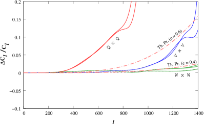
Figure 1: The predicted non-circular beam correction for a CMB experiment with elliptical Gaussian beam with fwhm beam-width of $0.22^{\circ}$ and two values of eccentricity, $e=0.6$ and $e=0.4$ are shown as dashed-dot lines (labeled Th. Pr.). The solid curves are the non circular beam corrections estimated by the WMAP team for the Q,V and W channels. The fwhm beam-width of $0.22^{\circ}$ corresponds closely to the cleanest and highest resolution W-band beam-width. For larger beam-widths, the theoretical curves would roughly shift left in multipole by the ratio of beam-widths.

To avoid contamination of the primordial CMB signal by Galactic emission, the region adjoining the Galactic plane is masked from maps. If the Galactic cut is small enough, then the coupling matrix will be invertible, and the two-point correlation function can be determined on all angular scales from the data within the uncut sky mch02 . Hivon et al. master present a technique (MASTER) for fast computation of the power spectrum taking accounting for the galactic cut, but for circular beams. In our present work, we present analytical expressions for the bias matrix of the Pseudo-${C_{l}}$ estimator for the incomplete sky coverage, using a non-circular beam.

2 CMB angular Power spectrum estimation: Non-circular beam & Non-uniform coverage effects

The observed CMB temperature fluctuation is convolved with a beam function and contaminated by noise. Further, the CMB signal cannot be obtained for full sky because of galactic contamination (and extragalactic point sources). We derive the general form of the bias matrix including non-uniform/incomplete sky coverage and a general beam function.

The observed temperature fluctuation field $\widetilde{\Delta T}(\mathbf{\hat{q}})$ is the convolution of the “beam” profile $B(\mathbf{\hat{q}},\mathbf{\hat{q}^{\prime}})$ with the real temperature fluctuation field $\Delta T(\mathbf{\hat{q}})$ (ignoring the additive noise term for simplicity) :

$$\widetilde{\Delta T}(\mathbf{\hat{q}})\ =\ \int_{4\pi}d\Omega_{\mathbf{\hat{q}^{\prime}}}\,B(\mathbf{\hat{q}},\mathbf{\hat{q}^{\prime}})\,\Delta T(\mathbf{\hat{q}^{\prime}}).$$ (1)

The two point correlation function for a statistically isotropic CMB anisotropy signal is

$$C(\mathbf{\hat{q}},\mathbf{\hat{q}}^{\prime})=\langle\widetilde{\Delta T}(\mathbf{\hat{q}})\widetilde{\Delta T}(\mathbf{\hat{q}^{\prime}})\rangle=\sum^{\infty}_{l=0}{(2l+1)\over 4\pi}\,C_{l}\,\,W_{l}(\mathbf{\hat{q}},\,\mathbf{\hat{q}}^{\prime})\,,$$ (2)

where $C_{l}$ is the angular spectrum of CMB anisotropy signal and the window function

$$W_{l}(\mathbf{\hat{q}}_{1},\mathbf{\hat{q}}_{2})\ \equiv\ \int d\Omega_{\mathbf{\hat{q}}}\int d\Omega_{\mathbf{\hat{q}^{\prime}}}\,B(\mathbf{\hat{q}}_{1},\mathbf{\hat{q}})B(\mathbf{\hat{q}}_{2},\mathbf{\hat{q}^{\prime}})P_{l}(\mathbf{\hat{q}}\cdot\mathbf{\hat{q}^{\prime}}),$$ (3)

encodes the effect of finite resolution through the beam function. A CMB anisotropy experiment probes a range of angular scales characterized by a window function $W_{l}(\mathbf{\hat{q}},\mathbf{\hat{q}}^{\prime})$. The window depends both on the scanning strategy as well as the angular resolution and response of the experiment. However, it is neater to logically separate these two effects by expressing the window $W_{l}(\mathbf{\hat{q}},\mathbf{\hat{q}}^{\prime})$ as a sum of ‘elementary’ window function of the CMB anisotropy at each point of the map TR:2001 . For a given scanning strategy, the results can be readily generalized using the representation of the window function as sum over elementary window functions (see, e.g., TR:2001 ; pyV ).

For some experiments, the beam function may be assumed to be circularly symmetric about the pointing direction, i.e., $B(\mathbf{\hat{q}},\mathbf{\hat{q}}^{\prime})\equiv B(\mathbf{\hat{q}}\cdot\mathbf{\hat{q}}^{\prime})$ without significantly affecting the results of the analysis. In any case, this assumption allows a great simplification since the beam function can then be represented by an expansion in Legendre polynomials as

$$B(\mathbf{\hat{q}}\cdot\mathbf{\hat{q}^{\prime}})\ =\ \frac{1}{4\pi}\,\sum_{l=0}^{\infty}\,(2l+1)\,B_{l}\,P_{l}(\mathbf{\hat{q}}\cdot\mathbf{\hat{q}^{\prime}}).$$ (4)

Consequently, it is straightforward to derive the well known simple expression

$$W_{l}(\mathbf{\hat{q}},\,\mathbf{\hat{q}^{\prime}})\ =\ B^{2}_{l}\,P_{l}(\mathbf{\hat{q}}\cdot\mathbf{\hat{q}^{\prime}})\,,$$ (5)

for a circularly symmetric beam function.

We define the Pseudo-$C_{l}$ estimator as

$$\widetilde{{C}}_{l}\ \equiv\ \frac{1}{4\pi}\int_{4\pi}d\Omega_{\mathbf{\hat{q}}_{1}}\int_{4\pi}d\Omega_{\mathbf{\hat{q}}_{2}}\,U(\mathbf{\hat{q}}_{1})\,U(\mathbf{\hat{q}}_{2})\,P_{l}(\mathbf{\hat{q}}_{1}\cdot\mathbf{\hat{q}}_{2})\,\widetilde{\Delta T}(\mathbf{\hat{q}}_{1})\,\widetilde{\Delta T}(\mathbf{\hat{q}}_{2}),$$ (6)

where $U(\mathbf{\hat{q}})$ denotes the mask function representing the incomplete sky. The expectation value of the Pseudo-$C_{l}$ estimator can be shown to take the form

$$\!\!\!\langle\widetilde{{C}}_{l}\rangle=\frac{1}{2l+1}\sum_{{l^{\prime}}=0}^{\infty}{C}_{l^{\prime}}\sum_{n=-l}^{l}\!\sum_{m=-{l^{\prime}}}^{l^{\prime}}\!\left|\int_{4\pi}\!\!\!d\Omega_{\mathbf{\hat{q}}}U(\mathbf{\hat{q}})\,Y_{ln}(\mathbf{\hat{q}})\left[\int_{4\pi}\!\!\!d\Omega_{\mathbf{\hat{q}^{\prime}}}\,Y^{*}_{{l^{\prime}}m}(\mathbf{\hat{q}^{\prime}})\,B(\mathbf{\hat{q}},\mathbf{\hat{q}^{\prime}})\right]\right|^{2}.$$ (7)

The integral in the square bracket can be simplified to TR:2001

$$\int_{4\pi}d\Omega_{\mathbf{\hat{q}^{\prime}}}\,Y^{*}_{{l^{\prime}}m}(\mathbf{\hat{q}^{\prime}})\,B(\mathbf{\hat{q}},\mathbf{\hat{q}^{\prime}})\ =\ \sqrt{\frac{2{l^{\prime}}+1}{4\pi}}\sum_{m^{\prime}=-{l^{\prime}}}^{l^{\prime}}B_{l^{\prime}}\,\beta_{{l^{\prime}}m^{\prime}}\,D^{l^{\prime}}_{mm^{\prime}}(\mathbf{\hat{q}},\rho(\mathbf{\hat{q}})).$$ (8)

The Beam Distortion Parameter (BDP) $\beta_{lm}\equiv b_{lm}/b_{l0}$ is expressed in terms of

$$b_{lm}\equiv\int_{4\pi}d\Omega_{\mathbf{\hat{q}}}\,Y_{lm}^{*}({\mathbf{\hat{q}}})\,B(\mathbf{\hat{z}},\mathbf{\hat{q}})\,,$$

$$B_{l}\equiv\int_{-1}^{1}d(\mathbf{\hat{q}}\cdot\mathbf{\hat{q}^{\prime}})\,P_{l}(\mathbf{\hat{q}}\cdot\mathbf{\hat{q}^{\prime}})\,\mathcal{B}(\mathbf{\hat{q}}\cdot\mathbf{\hat{q}^{\prime}})$$ (9)

where $\mathcal{B}(\mathbf{\hat{q}}\cdot\mathbf{\hat{q}^{\prime}})$ is the circularized beam obtained by averaging $B(\mathbf{\hat{z}},\mathbf{\hat{q}})$ over azimuth $\phi$. Hence,

$$B_{l}=\int_{0}^{\pi}\sin\theta d\theta\,\sqrt{\frac{4\pi}{2l+1}}\,Y_{l0}^{*}({\mathbf{\hat{q}}})\left[\frac{1}{2\pi}\int_{0}^{2\pi}d\phi\,B(\mathbf{\hat{z}},\mathbf{\hat{q}})\right]=\sqrt{\frac{4\pi}{2l+1}}\,b_{l0}.$$

Making a spherical harmonic expansion of the mask function $U(\mathbf{\hat{q}})$

$$U(\mathbf{\hat{q}})\ =\ \sum_{l=0}^{\infty}\sum_{m=-l}^{l}U_{lm}\,Y_{lm}(\mathbf{\hat{q}})$$ (10)

we can simplify Eq.7 as

$$\langle\widetilde{{C}}_{l}\rangle\ =\ \sum_{{l^{\prime}}}A_{l{l^{\prime}}}C_{l^{\prime}}\,.$$ (11)

The general form of the bias matrix, $A_{l{l^{\prime}}}$ is thus given by

$$A_{ll^{\prime}}\ =\ \frac{B_{l}^{2}}{4\pi}\frac{(2l^{\prime}+1)}{(2l+1)}\sum_{n=-l}^{l}\sum_{m=-l^{\prime}}^{l^{\prime}}\left|\sum_{m^{\prime}=-l^{\prime}}^{l^{\prime}}\beta_{l^{\prime}m^{\prime}}\sum_{{l^{\prime\prime}}=0}^{\infty}\sum_{m^{\prime\prime}=-{l^{\prime\prime}}}^{{l^{\prime\prime}}}U_{{l^{\prime\prime}}m^{\prime\prime}}\,J^{l{l^{\prime\prime}}{l^{\prime}}}_{nm^{\prime\prime}mm^{\prime}}\right|^{2},$$ (12)

where

$$J^{l{l^{\prime\prime}}{l^{\prime}}}_{nm^{\prime\prime}mm^{\prime}}\ \equiv\ \int_{4\pi}d\Omega_{\mathbf{\hat{q}}}\,Y_{ln}(\mathbf{\hat{q}})\,Y_{{l^{\prime\prime}}m^{\prime\prime}}(\mathbf{\hat{q}})\,D_{mm^{\prime}}^{l^{\prime}}(\mathbf{\hat{q}},\rho(\mathbf{\hat{q}})).$$ (13)

To proceed further analytically, we need a model for $\rho(\mathbf{\hat{q}})$. We shall continue assuming non-rotating beams, i.e. $\rho(\mathbf{\hat{q}})=0$. We evaluate the integral $J^{l{l^{\prime\prime}}{l^{\prime}}}_{nm^{\prime\prime}mm^{\prime}}$, with two different approaches. In the first method, using only the sinusoidal expansion of Wigner-$d$, we get

$$J^{l{l^{\prime\prime}}{l^{\prime}}}_{nm^{\prime\prime}mm^{\prime}} = 2\pi\,\delta_{m^{\prime\prime}(m-n)}\frac{\sqrt{(2l+1)(2{l^{\prime\prime}}+1)}}{4\pi}\sum_{M=-l}^{l}d^{l}_{nM}\left(\frac{\pi}{2}\right)d^{l}_{M0}\left(\frac{\pi}{2}\right)$$ (14)

$${}\times\sum_{{M^{\prime\prime}}=-{l^{\prime\prime}}}^{{l^{\prime\prime}}}d^{{l^{\prime\prime}}}_{m^{\prime\prime}{M^{\prime\prime}}}\left(\frac{\pi}{2}\right)d^{{l^{\prime\prime}}}_{{M^{\prime\prime}}0}\left(\frac{\pi}{2}\right)\sum_{M^{\prime}=-{l^{\prime}}}^{{l^{\prime}}}d^{{l^{\prime}}}_{mM^{\prime}}\left(\frac{\pi}{2}\right)d^{{l^{\prime}}}_{M^{\prime}m^{\prime}}\left(\frac{\pi}{2}\right)$$

$${}\times\left[i^{n+m+m^{\prime}+m^{\prime\prime}}\,(-1)^{M+{M^{\prime\prime}}+M^{\prime}}\int_{0}^{\pi}\sin\theta d\theta\,e^{i(M+M^{\prime}+{M^{\prime\prime}})\theta}\right].$$

In the alternative method using Clebsch Gordon coefficients, we can evaluate $J^{l{l^{\prime\prime}}{l^{\prime}}}_{nm^{\prime\prime}mm^{\prime}}$ as:

$$J^{l{l^{\prime\prime}}{l^{\prime}}}_{nm^{\prime\prime}mm^{\prime}} =(-1)^{n+m^{\prime\prime}}\,\delta_{m^{\prime\prime}(m-n)}\,\frac{\sqrt{(2l+1)(2{l^{\prime\prime}}+1)}}{2}$$ (15)

$$\times\sum_{L=|l-{l^{\prime\prime}}|}^{l+{l^{\prime\prime}}}C^{L0}_{l0{l^{\prime\prime}}0}C^{L(n+m^{\prime\prime})}_{ln{l^{\prime\prime}}m^{\prime\prime}}\sum_{{L^{\prime}}=|L-{l^{\prime}}|}^{L+{l^{\prime}}}C^{{L^{\prime}}(m-n-m^{\prime\prime})}_{L(-n-m^{\prime\prime}){l^{\prime}}m}\,C^{{L^{\prime}}m^{\prime}}_{L0{l^{\prime}}m^{\prime}}$$

$$\times\sum_{N=-{L^{\prime}}}^{{L^{\prime}}}\,d^{{L^{\prime}}}_{0N}\left(\frac{\pi}{2}\right)\,d^{{L^{\prime}}}_{Nm^{\prime}}\left(\frac{\pi}{2}\right)\,\left[i^{m^{\prime}}\,(-1)^{N}\int_{0}^{\pi}\sin\theta d\theta\,e^{iN\theta}\right].$$

The analytic expressions reduce to the known analytical results for circular beam and non-uniform sky coverage studied in ref. master and our earlier results for non-circular beam for full sky mit04 .

These results offer the possibility of rapid estimation of the non-circular beam effect in the Pseudo-$C_{l}$ estimation. The expression in terms of the $d_{mm^{\prime}}^{l}(\pi/2)$ coefficients is the computationally superior approach. These coefficients can be computed using stable recurrence relations ris96 ; wan_gor01 . In a more detailed publication we describe the algorithm in more detail usinprep . The expressions also highlight the two aspects to speeding up the computation of the systematic effect:

• Mildly non-circular beams where the beam distortion parameters (BDP), $\beta_{lm}$ at each $l$ fall off rapidly with $m$. This allows us to neglect $\beta_{lm}$ for $m>m_{\mathrm{b}eam}$. For most real beams, $m_{\mathrm{beam}}\sim 4$ is a sufficiently good approximation. This cuts-off the summations over BDP in the expressions for $A_{l{l^{\prime}}}$.

• Soft, azimuthally apodized, masks where the coefficients $U_{lm}$ are small beyond $m>m_{\mathrm{mask}}$. Moreover, it is useful to smooth the mask in $l$, such the $U_{lm}$ die off rapidly for $l>l_{\mathrm{mask}}$ too.

The mild-circularity perturbation approach has been introduced and discussed in ref. TR:2001 . The circularity of the beam has to be addressed in the design of the CMB experiments. Our results suggest the systematics due to non-circular distortions of the beam are manageable if one ensures the large BDP are limited to a few $m$ (i.e., narrow band limited violation of axis-symmetry). The beams for many experiments, such as Python-V and WMAP are well approximated as elliptical Gaussian functions TR:2001 ; pyV ; mit04 . For radically non-axisymmetric beams, modeling the beam in terms of superposition of displaced circular Gaussian beams has been proposed asym_04 ; xspect_05 . Our approach allows a simple, cost effective extension to modeling with the more general elliptical Gaussian beams, or other mildly non-circular beam forms.

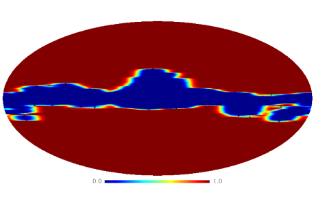
Figure 2: A softened (azimuthally smoothed) mask reconstructed from the WMAP Kp2 mask which would reduce the computational cost of estimating the non-circular beam effect on the angular power spectrum.

The mask of the galactic region $U(\mathbf{\hat{q}})$ can be chosen at the time of data analysis. The coupling of BDP with $U_{lm}$ suggests that a judicious choice of mask reduces the computational costs of non-circular beam corrections. Fig. 2 shows a softened version of the Kp2 mask used by the WMAP team Bennett1 , where the mask is azimuthally smoothed. The final apodized mask is obtained by multiplying an azimuthally smoothed mask raised to a sufficiently large power with the original mask and has reduced power at large $m$ (i.e., $U_{lm}$ is negligible for $m>m_{\mathrm{mask}}$) . In a forthcoming publication we describe the method of making soft masks usinprep . For mildly non-circular, nearly azimuthally symmetric case, the required number of computation cycle to compute the bias matrix up to a multipole $l$ scales as $\sim(2m_{\mathrm{beam}}+1)(2m_{\mathrm{mask}}+1)\,l^{5}$ up to leading order for $l\gg l_{\mathrm{mask}}$. Here, $m_{\mathrm{beam}}$ is the cut-off in the beam distortion parameters (BDP), $\beta_{lm}$ and $m_{\mathrm{mask}}$ is the cut-off in $U_{lm}$.

3 Discussion & Conclusion

The assumptions of non-circular beam leads to major complications at every stage of the data analysis pipeline. The extent to which the non-circularity affects the step of going from the time-stream data to sky map is very sensitive to the scan-strategy. The beam now has an orientation with respect to the scan path that can potentially vary along the path. This implies that the beam function is inherently time dependent and difficult to deconvolve.

We extend our analytic approach for addressing the effect of non-circular experimental beam function in the estimation of the angular power spectrum $\mathcal{C}_{l}$ of CMB anisotropy, which also includes the effect of the galactic cut in the entire sky map. Non-circular beam effects can be modeled into the covariance functions in approaches related to maximum likelihood estimation max97 ; bjk98 and can also be included in the Harmonic ring harm02 and ring-torus estimators wan_han03 . However, all these methods are computationally prohibitive for high resolution maps and, at present, the computationally economical approach of using a Pseudo-$C_{l}$ estimator appears to be a viable option for extracting the power spectrum at high multipoles efs04 . The Pseudo-$C_{l}$ estimates have to be corrected for the systematic biases. While considerable attention has been devoted to the effects of incomplete/non-uniform sky coverage, no comprehensive or systematic approach is available for non-circular beam. The high sensitivity, ‘full’ (large) sky observation from space (long duration balloon) missions have alleviated the effect of incomplete sky coverage and other systematic effects such as the one we consider here have gained more significance. Non-uniform coverage, in particular, the galactic masks affect only CMB power estimation at the low multipoles. The analysis accompanying the recent second data from WMAP uses the hybrid strategy efs04 where the power spectrum at low multipoles is estimated using optimal Maximum Likelihood methods and Pseudo-$C_{l}$ are used for large multipoles hin_wmap06 ; sperg_wmap06 .

The non-circular beam is an effect that dominates at large $l$ comparable to the inverse beam width mit04 . For high resolution experiments, the optimal maximum likelihood methods which can account for non-circular beam functions are computationally prohibitive. In implementing the Pseudo-$C_{l}$ estimation, we have included both the non-circular beam effect and the effect of non-uniform sky coverage. Our work provides a convenient approach for estimating the magnitude of these effects in terms of the leading order deviations from a circular beam and azimuthally symmetric mask. The perturbation approach is very efficient. For most CMB experiments the leading few orders capture most of the effect of beam non-circularity TR:2001 . Our results highlight the advantage of azimuthally smoothed masks (mild deviations from azimuthal symmetry) in reducing computational costs. The numerical implementation of our method can readily accommodate the case when pixels are revisited by the beam with different orientations. Evaluating the realistic bias and error-covariance for a specific CMB experiment with non-circular beams would require numerical evaluation of the general expressions for $A_{l{l^{\prime}}}$ using real scan strategy and account for inhomogeneous noise and sky coverage, the latter part of which has been addressed in this present work.

It is worthwhile to note in passing that that the angular power $C_{l}$ contains all the information of Gaussian CMB anisotropy only under the assumption of statistical isotropy. Gaussian CMB anisotropy map measured with a non-circular beam corresponds to an underlying correlation function that violates statistical isotropy. In this case, the extra information present may be measurable using, for example, the bipolar power spectrum haj_sour03 ; haj_sour05 ; haj_sour06 ; bas06 . Even when the beam is circular the scanning pattern itself is expected to cause a breakdown of statistical isotropy of the measured CMB anisotropy  master . For a non-circular beam, this effect could be much more pronounced and, perhaps, presents an interesting avenue of future study.

In addition to temperature fluctuations, the CMB photons coming from different directions have a random, linear polarization. The polarization of CMB can be decomposed into $E$ part with even parity and $B$ part with odd parity. Besides the angular spectrum $C_{l}^{TT}$, the CMB polarization provides three additional spectra, $C_{l}^{TE}$, $C_{l}^{EE}$ and $C_{l}^{BB}$ which are invariant under parity transformations. The level of polarization of the CMB being about a tenth of the temperature fluctuation, it is only very recently that the angular power spectrum of CMB polarization field has been detected. The Degree Angular Scale Interferometer (DASI) has measured the CMB polarization spectrum over limited band of angular scales in late 2002 kov_dasi02 . The DASI experiment recently published 3-year results of much refined measurements dasi_3y . More recently, the BOOMERanG collaboration reported new measurements of CMB anisotropy and polarization spectra boom_polar . The WMAP mission has also measured CMB polarization spectra  kog_wmap03 ; pag_wmap06 . Correcting for the systematic effects of a non-circular beam for the polarization spectra is expected to become important. Extending this work to the case CMB polarization is another line of activity we plan to undertake in the near future.

In summary, we have presented a perturbation framework to compute the effect of non-circular beam function on the estimation of power spectrum of CMB anisotropy taking into account the effect of a non-uniform sky coverage (eg., galactic mask). We not only present the most general expression including non-uniform sky coverage as well as a non-circular beam that can be numerically evaluated but also provide elegant analytic results in interesting limits. As CMB experiments strive to measure the angular power spectrum with increasing accuracy and resolution, the work provides a stepping stone to address a rather complicated systematic effect of non-circular beam functions.

References

- (1) J. R. Bond, Theory and Observations of the Cosmic Background Radiation, in Cosmology and Large Scale Structure, Les Houches Session LX, August 1993, ed. R. Schaeffer, (Elsevier Science Press, 1996).
- (2) W. Hu and S. Dodelson, Ann. Rev. of Astron. and Astrophys. 40, 171 (2002).
- (3) G. Efstathiou, Mon. Not. Roy. Astron. Soc. 349, 603 (2004).
- (4) K. M. Gorski, Astrophys. J. Lett., 430, L85, (1994).
- (5) K. M. Gorski, et.al., Astrophys. J. Lett., 430, L89, (1994).
- (6) K. M. Gorski, et.al., Astrophys. J. Lett., 464, L11, (1996).
- (7) K. M. Gorski, in the Proceedings of the XXXIst Recontres de Moriond,‘Microwave Background Anisotropies’, (1997); astro-ph/9701191.
- (8) M. Tegmark, Phys. Rev. D55, 5895, (1997).
- (9) J. R. Bond, A. H. Jaffe and L. Knox, Phys. Rev. D 57, 2117, (1998).
- (10) J. Borrill, Phys. Rev. D 59, 27302 (1999); J. Borrill in Proceedings of the 5th European SGI/Cray MPP Workshop, (1999); astro-ph/9911389.
- (11) J. R. Bond, R. G. Crittenden, A. H. Jaffe, L. Knox, Comput.Sci.Eng. 1, 21 (1999).
- (12) S. P. Oh, D. N. Spergel and G. Hinshaw, Astrophys. J. 510, 551, (1999).
- (13) O. Dore, L.Knox and A. Peel, Phys. Rev. D 64, 3001, (2001).
- (14) U. L. Pen, Mon. Not. Roy. Astron. Soc., 346, 619, (2001).
- (15) A. D. Challinor et al., Mon. Not. Roy. Astron. Soc. 331, 994, (2002); F. van Leeuwen et al., Mon. Not. Roy. Astron. Soc. 331, 975, (2002).
- (16) B. D. Wandelt and F. Hansen, Phys. Rev. D 67, 23001, (2003).
- (17) L. Knox, N. Christensen & C. Skordis, Astrophys. J.563, L95, (2001).
- (18) B. D. Wandelt, D. L. Larson & A. Lakshminarayanan, Phys. Rev. D. 70, 083511 (2004).
- (19) J. Jewell, S. Levin & C.H. Anderson, Astrophys. J.609, 1, (2004).
- (20) J. T. Yu and P. J. E. Peebles, Astrophys. J. 158, 103, (1969).
- (21) P. J. E. Peebles, Astrophys. J. 185, 431, (1974).
- (22) B. Wandelt, E. Hivon and K. M. Gorski, Phys. Rev. D 64, 083003 (2003).
- (23) I. Szapudi, S. Prunet, D. Pogosyan, A. Szalay, J. R. Bond, Astrophys. J. 548, L115, (2001).
- (24) I. Szapudi, S. Prunet, S. Colombi, Astrophys. J. 561, L11, (2001).
- (25) C. L. Bennett et.al., Astrophys. J. Suppl., 148, 1, (2003).
- (26) G. Hinshaw et.al., Astrophys. J. Suppl.,148, 135, (2003).
- (27) E. Hivon, K. M. Gorski, C. B. Netterfield, B. P. Crill, S. Prunet and F. Hansen, Astrophys. J. 567, 2, (2002).
- (28) M. L. Brown, P. G. Castro, A. N. Taylor, Mon.Not.Roy.Astron.Soc. 360, 1262, (2005).
- (29) S. Mitra, A. S. Sengupta and T. Souradeep, Phys. Rev. D 70, 103002 (2004).
- (30) T. Souradeep and B. Ratra, Astrophys. J.560 28 (2001)
- (31) P. Fosalba, O. Dore and F. R. Bouchet, Phys. Rev. D 65, 063003 (2002).
- (32) D. J. Mortlock, A. D. Challinor and M. P. Hobson, Mon. Not. Roy. Astron. Soc. 330, 405 (2002).
- (33) K. Coble et al., Astrophys. J. 584, 585, (2003); P. Mukherjee et al., Astrophys. J. 592, 692, (2003).
- (34) T. Risbo, Journal of Geodesy, 70, 383, (1996).
- (35) B. D. Wandelt and K. M.Gorski, Phys. Rev. D 63, 123002 (2001).
- (36) M. Tristram, J.-C. Hamilton, J. F. Macias-Perez, C. Renault, Phys. Rev. D 69, 063003 (2004).
- (37) M. Tristram, J. F. Macias-Perez, C. Renault, D. Santos, Mon. Not. Roy. Astron. Soc. 358, 883, (2005).
- (38) C. L. Bennett et al., Astrophys. J. Supp., 148, 97 (2003).
- (39) S. Mitra, A. Sengupta, S. Ray, R. Saha and Tarun Souradeep, in preparation.
- (40) G. Efstathiou, Mon. Not. Roy. Astron. Soc. 370, 343 (2006).
- (41) G. Hinshaw et al., preprint [arXiv: astro-ph/0603451].
- (42) D. Spergel et al., preprint [arXiv: astro-ph/0603449].
- (43) A. Hajian and T. Souradeep, Astrophys. J. 597, L5 (2003).
- (44) A. Hajian & T. Souradeep & N. Cornish, Astrophys. J. Lett. 618, L63 (2005).
- (45) A. Hajian & T. Souradeep, preprint [arXiv:astro-ph/0607153].
- (46) S. Basak, A. Hajian & T. Souradeep, Phys. Rev. D 74, 021301(R) (2006).
- (47) J. M. Kovac et al., Nature 420, 772, (2002).
- (48) E. M. Leitch, J. M. Kovac, N. W. Halverson, J. E. Carlstrom, C. Pryke and M. W. E. Smith ApJ 624, 10, (2005).
- (49) F. Piacentini et al. 2005 Preprint astro–ph/0507507; C. J. MacTavish et al. 2005 Preprint astro–ph/0507503.
- (50) A. Kogut, et.al., Astrophys.J.Suppl., 148, 161 (2003).
- (51) L. Page et al., preprint, [arXiv:astro-ph/0603450].