A combined re-analysis of existing blank-field SCUBA surveys: comparative $\bf 850-\mu m$ source lists, combined number counts, and evidence for strong clustering of the bright sub-mm galaxy population on arcminute scales.

Abstract

Since the advent of SCUBA on the JCMT, a series of complementary surveys has resolved the bulk of the far-infrared extragalactic background into discrete sources. This has revealed a population of heavily dust-obscured sources at high redshift ($z>1$) undergoing an intense period of massive star-forming activity with inferred star formation rates of several hundred to several thousand solar masses per year. Taken together, these existing surveys cover a total area of 460 sq. arcmin to a range of depths, but combining the results has hitherto been complicated by the fact that different survey groups have used different methods of data reduction and source extraction. In this paper we re-reduce and analyse all of the blank field surveys to date in an almost identical manner to that employed in the “SCUBA 8 mJy Survey”. Comparative source catalogues are given which include a number of new significant source detections as well as failing to confirm some of those objects previously published. These new source catalogues have been combined to produce the most accurate number counts to date from 2 to 12.5 mJy. We find $\rm N(>4\,mJy)=620^{+110}_{-190}\,deg^{-2}$, $\rm N(>6\,mJy)=310^{+\phantom{0}60}_{-100}\,deg^{-2}$, $\rm N(>8\,mJy)=150^{+\phantom{0}40}_{-\phantom{0}60}\,deg^{-2}$ and $\rm N(>10\,mJy)=\phantom{0}40^{+\phantom{0}20}_{-\phantom{0}20}\,deg^{-2}$ after correcting for the effects of incompleteness, flux-density boosting and contamination from spurious / confused detections. Furthermore the cumulative number counts appear to steepen beyond $\rm S_{850}>8\,mJy$, which could indicate an intrinsic turn-over in the underlying luminosity function placing an upper limit on the luminosity (and hence mass) of a high redshift galaxy. We have also investigated the clustering properties of the bright $\rm S_{850}>5\,mJy$ SCUBA population by means of 2-point angular correlation functions. We find a $\rm\simeq 3.5\sigma$ excess of pairs within the first 100 arcsec over that expected from a Poisson distribution. Fits of a standard power-law of the form $\rm w(\theta)=A\theta^{-\delta}$ to the angular correlation functions for $\rm S_{850}>5\,mJy$ are limited in accuracy by the small number of source detections but appear to be broadly consistent with that measured for EROs. Nearest-neighbour analyses further support strong clustering on arcmin scales, rejecting the null hypothesis that the distribution of the submm sources is random at the 95% confidence level for $\rm S_{850}>5\,mJy$, and at the 99% confidence level for $\rm S_{850}>7\,mJy$.

1 Introduction

Over the past seven years, a series of complementary deep $850\,{\rm\mu m}$ surveys (eg. Smail et al. 1997, Hughes et al. 1998, Blain et al. 1999, Barger et al. 1998, Barger et al. 1999, Eales et al. 2000, Scott et al. 2002, Cowie et al. 2002, Borys et al. 2003, Webb et al. 2003a) carried out using SCUBA (Holland et al. 1999) on the JCMT has resolved the bulk of the far-infrared (FIR) extragalactic background into discrete sources. These surveys vary in size and depth from ultra-deep surveys exploiting gravitational lensing from intervening clusters to study the very faintest submm sources (Smail et al. 1997, Cowie et al. 2002), small and deep blank field surveys such as the HDF (6 sq. arcmin to a uniform $1\sigma_{\rm rms}\simeq 0.5$ mJy/beam; Hughes et al. 1998, Serjeant et al. 2003), through to moderate area and comparatively shallower blank field surveys such as the “SCUBA 8-mJy Survey” (a total of 250 sq. arcmin to a uniform $1\sigma_{\rm rms}\simeq 2.5$ mJy/beam; Scott et al. 2002). These surveys have revealed a population of heavily dust-enshrouded high-redshift ($z>1$) morphologically-irregular galaxies. Although there is still considerable uncertainty in the fraction of SCUBA sources hosting either low luminosity or Compton-thick AGNs (Smail et al. 2002, Ivison et al. 2002), deep X-ray observations with the Chandra and XMM-Newton telescopes have suggested that even when an AGN is present, it rarely dominates the far-infrared / submillimetre emission from the galaxy (Frayer et al. 1998, Alexander et al. 2003). Hence, if the thermal dust emission is dominated by reprocessed starlight, the inferred star formation rates (SFRs) in the very brightest submillimetre galaxies may be as high as several thousand solar masses per year. This is sufficient to form the most massive elliptical galaxies observed in the present-day Universe on timescales of $\sim 1$ Gyr, implying that the submillimetre sources may be the progenitors of todays massive ellipticals, and that the star-formation rate density in the early Universe was at least a factor of 2 larger than that derived from optical / UV observations (Steidel et al. 1999).

A key test of whether the bright submillimetre sources really are the progenitors of present-day massive spheroids is to measure their clustering properties. If they are indeed proto-massive ellipticals then they should be strongly clustered. This is an inevitable result of gravitational collapse from Gaussian initial density fluctuations: the rare high-mass peaks are strongly biased with respect to the mass (eg. Benson et al. 2001). Each of the submillimetre survey consortia have performed their own reduction, source extraction and simulations on their individual datasets, in order to study the nature of the SCUBA population in general. However, each survey alone images only $\sim 100-200$ sq. arcmin of sky spread over several fields, resulting in discrepancies in the cumulative number counts at $\rm S_{850}>8\,mJy$ by over a factor of 5 due to cosmic variance, and also potentially the effects of clustering. Furthermore, no individual survey has identified enough sources to make a significant measurement of the clustering properties, although tentative evidence was obtained for strong clustering on scales of 1-2 arcmin from the “SCUBA 8 mJy Survey”, the largest of these surveys undertaken to date (Scott et al. 2002).

In this paper we combine the data from all of the blank field surveys completed up to the completion date of the “SCUBA 8 mJy Survey”. In order to do this we downloaded the raw data for the “Canada UK Deep Submillimetre Survey (CUDSS)”, the “Hawaii Flanking Fields Survey” and the “Hubble Deep Field (HDF) North Pencil Beam Survey” from the Canadian Astronomy Data Centre (CADC) archive and re-reduced it in an identical manner to that employed in the “SCUBA 8 mJy Survey”. This is decribed in Section 2. The source extraction algorithm developed by Scott et al. (2002) was used to identify significant submillimetre sources in each of the fields, and this method is described briefly in Section 3. In Section 4 we present and discuss the results of simulations carried out both in conjunction with the real data, and through the production of fully-simulated survey areas, for all of the survey fields. Comparative reduction methods and source lists down to a signal-to-noise ratio of 3.00 are given in Section 5. These lists include some previously unidentified significant sources but also cast doubt on the reality of other published detections. Section 6 combines these new catalogues into a master source list, from which the most accurate cumulative number counts to date in the flux density range $2-12.5$ mJy have been calculated. A number of models are tested against these data points. In Section 7, the new master catalogue has been used in an attempt to measure the clustering properties of the bright ($>5$ mJy) submillimetre sources, through 2-point angular correlation functions and nearest-neighbour analyses. Section 8 outlines the resulting motivation and aims of the current blank field survey work being undertaken by the JCMT + SCUBA, and the conclusions from this work are presented in Section 9.

2 Data Reduction

The raw data for the “Canada UK Deep Submillimetre Survey (CUDSS)”, the “Hawaii Flanking Fields Survey”, and the “Hubble Deep Field Survey” (pencil beam only) were downloaded from the Canadian Astronomy Data Centre (CADC) archive. The data were then fully reduced using the same Interactive Data Language (IDL)-based reduction routines employed in the “SCUBA 8 mJy Survey”. This procedure is fully described in Scott et al. (2002), but is summarised briefly below.

Firstly, in order to take nodding into consideration, the off-position was subtracted from the on-position in the raw beam-switched data. The relative sensitivities of the bolometers, with respect to a reference bolometer (the central bolometers H7 and C14, for the $\rm 850\,\mu m$ and $\rm 450\,\mu m$ arrays respectively) were accounted for by multiplying by the standard flatfield values. The atmospheric opacity was measured wherever possible using a 6th order polynomial fit to the 225 GHz measurements from the Caltech Submillimetre Observatory (CSO), followed by a linear interpolation to 850 and $\rm 450\,\mu m$ using the relations given in Archibald et al. (2002a). On the occasions when the CSO opacity meter was out of service, or less than 7 reliable CSO observations were available within $\pm 1$ hour of each observation, a linear interpolation between successive skydip values was used to determine $\rm\tau_{850\mu m}$ and $\rm\tau_{450\mu m}$.

The next stage in the data reduction process was to remove spikes in the data resulting from cosmic-rays and bad bolometers, and to remove any residual sky emission. In this IDL reduction, deglitching and residual sky subtraction were undertaken by an iterative process, each iteration making a temporal noise estimate and deglitching, followed by a spatial sky subtraction. There were no bright sources in any of submm survey fields that would have been significantly detected in any single jigglemap, let alone in sub-dividing the data-stream into shorter timescale chunks and so the procedure was as follows:

$\bullet$ For each bolometer, noise estimates were made by fitting a Gaussian to the data-stream in chunks of 128 readout groups.

$\bullet$ These time dependent noise estimates were then used to remove any spikes by performing a $\rm 3\sigma$ clip on the data.

$\bullet$ Using the fits to all of the bolometers in the array, a modal residual sky level was determined for each of these 128 readout groups, and subtracted from these data.

With each consecutive iteration, the deglitching process makes a harder cut. Noisy bolometers were assigned a low inverse variance weight in this way. In the case of the calibration data, however, the presence of a bright source would likely lead to over-enthusiastic clipping of the data, and so in this case a timeline without object signal was constructed. This was created by calculating the mean of the timestream data points recorded immediately before and after the readout being considered, and subtracting this from the readout value.

Flux conversion factors (FCFs) were determined by dividing the flux density within the JCMT beam of a known calibration source by the measured peak voltage. Each of the individual jiggle-maps comprising the submm survey data were calibrated prior to producing the final coadded images using the gain value from whichever calibration source was taken closest in time.

The final images were produced using an optimal noise-weighted drizzling algorithm (Fruchter & Hook, 2002) with a pixel size of 1 sq. arcsec. This is the same method as that employed in the ‘SCUBA 8-mJy Survey’ (Scott et al. 2002) and ‘Hubble Deep Field North’ (Serjeant et al. 2003) data reductions. Both output signal and noise maps were created, the signal in any one sq. arcsec pixel given by the noise-weighted average of the bolometer readouts at that position, and the corresponding noise value given by a noise-weighted average of the Gaussian fits to the readout histograms. Unlike a standard shift-and-add technique which takes the flux density in each detector pixel and places it into the final map over an area equivalent to one detector pixel projected on the sky, drizzling takes the flux density and places it into a smaller area in the final map. Although this significantly reduces the signal-to-noise ratio in each pixel, this approach helps preserve information on small angular scales, provided that there are enough observations to fill in the resulting gaps. The area in the coadded map receiving the flux from one detector pixel is termed the ‘footprint’. This method is an extreme example of drizzling in which the ‘footprint’ is selected to be as small as is practicable given the pointing errors invloved (termed the ‘zero-footprint’), selected here to be one sq. arcsec. Unlike in the standard SURF reduction, there is no intrinsic smoothing or interpolation between neighbouring pixels in this rebin procedure. Although there is some degree of correlation between pixels in the output zero-footprint signal maps in terms of the beam pattern, the corresponding pixel noise values represent individual measurements of the temporally varying sky noise averaged over the dataset integration time, at a specific point on the sky, and are hence statistically independent from their neighbours. In essence this method produces a very oversampled image with statistically independent pixels. A final $4\sigma$-clip on the signal-to-noise was carried out to remove any remaining ‘hot pixels’. A noise-weighted convolution with a beam-sized Gaussian point spread function (PSF) was used to produce realistic smoothed maps of the survey areas whilst accounting for variable signal-to-noise between individual pixels.

3 Source Extraction

Survey	Total area	Uniform noise	$\rm 1\sigma$ rms noise
Field	/sq. arcmins	area /sq. arcmins	level mJy/beam
ELAIS N2	$137$	$113$	$2.2\pm 0.7$
Lockman Hole wide area	$\phantom{0}141$*	$\phantom{0}88$	$2.7\pm 0.7$
Lockman Hole deep strip		$\phantom{0}21$	$1.8\pm 0.2$
CUDSS 03h wide area	$\phantom{00}69$*	$\phantom{0}55$	$1.8\pm 0.5$
CUDSS 03h deep area		$\phantom{00}8$	$1.1\pm 0.2$
CUDSS 10h	$\phantom{0}10$	$\phantom{00}8$	$1.3\pm 0.2$
CUDSS 14h	$\phantom{0}61$	$\phantom{0}57$	$1.5\pm 0.3$
CUDSS 22h	$\phantom{00}7$	$\phantom{00}5$	$1.5\pm 0.3$
Hubble Deep Field	$\phantom{0}10$	$\phantom{00}6$	$0.6\pm 0.1$
SSA13 wide area	$\phantom{00}72$*	$\phantom{0}45$	$2.5\pm 0.6$
SSA13 deep area		$\phantom{00}8$	$0.7\pm 0.1$
SSA17	$\phantom{0}24$	$\phantom{0}21$	$1.6\pm 0.5$
SSA22	$\phantom{0}26$	$\phantom{0}21$	$0.9\pm 0.2$
Lockman Hole deep area	$\phantom{0}11$	$\phantom{00}8$	$0.8\pm 0.1$

Table 1: Survey field areas and $\rm 1\sigma$ rms noise levels in the regions of uniform noise, as given by the mean and standard deviation measured directly from the 14.5” FWHM Gaussian convolved noise maps. Total areas marked with * refer to fields composed of a small deep region within a wider shallower survey area and correspond to the full area of that entire field (ie. both shallow and deep).

The chopping-nodding mechanism of the telescope provides a valuable method of discriminating between real detections and spurious noise spikes in the data. With the exception of the Hubble Deep Field (HDF), each of the surveys used a single chop throw fixed in right ascension (RA), thus creating negative sidelobes, half the depth of the peak flux density, on either side of a real source. In the case of the HDF, this strategy was modified to use two chop throws fixed in RA, each chop throw used for approximately half of the total integration time. This side-lobe signal can be recovered to boost the overall signal-to-noise ratio of a detection.

For well-separated sources, convolving the images with the beam is formally the best method of source extraction (Eales et al. 1999, 2000, Serjeant et al. 2003). However, following a careful examination of the reduced “8 mJy Survey” data (Scott et al. 2002), it became clear that some of the potential sources were partially confused. This was particularly prominent in the map of ELAIS N2 where the negative sidelobes of individual sources have overlapped and are therefore somewhat deepened relative to both source peaks. Consequently, in order to decouple any confused sidelobes a source-extraction algorithm was devised based on a simultaneous maximum-likelihood fit to the flux densities of all potentially significant peaks in the maps. This is made feasible by the independent data-points and errors yielded by the zero-footprint IDL-reduced maps. These peaks were identified as any positive peak in the noise-weighted Gaussian convolved signal maps. Using a peak-normalised beam-map as a source template (generated by binning together all of the observations of Uranus or CRL618 taken with the relevant chop throw), a basic model was constructed by centring a beam-map at the positions of every peak in the maps. The normalisation coefficients of each of the positioned beam-maps were then calculated simultaneously such that the final multi-source model provided the best description of the submm sky, as judged by a minimum $\chi^{2}$ fit.

The fitting process is as follows. Suppose one considers a normalised beam-map $B(x,y)$ as a source template and that at position $(i,j)$ in the unconvolved image the signal is $S(i,j)$ and the noise is $N(i,j)$. If n peaks above a specified flux threshold are located in the Gaussian-convolved image, one may construct a model to the unconvolved zero-footprint image such that beam-maps centred on each peak position are simultaneously scaled to give an overall best fit to the entire image. Using a minimum $\chi^{2}$ fit as the maximum likelihood estimator then

$$\chi^{2}=\left(\sum_{i,j}\frac{S(i,j)-\sum_{k=1}^{n}a_{k}B_{k}(x-i,y-j)}{N(i,j)^{2}}\right)^{2}$$ (1)

where $a_{k}$ is the best fit flux to the $k$th peak.

Defining $\alpha_{mk}$, an $n\times n$ matrix, as

$$\alpha_{mk}=\sum_{i,j}\frac{B_{k}(x-i,y-j)B_{m}(x-i,y-j)}{N(i,j)^{2}}$$ (2)

and $\beta_{m}$, a vector of length $n$ as

$$\beta_{m}=\sum_{i,j}\frac{S(i,j)B_{m}(x-i,y-j)}{N(i,j)^{2}}$$ (3)

then the best fit values of $a_{k}$ are given by

$$a_{k}=\sum_{m=1}^{n}[\alpha]_{km}^{-1}\beta_{m}$$ (4)

and the significances $\sigma(a_{k})$ of the peak detections are given by

$$\sigma(a_{k})=\frac{a_{k}}{\sqrt{[\alpha]_{kk}^{-1}}}$$ (5)

Furthermore, this method can be modified to deal with surveys which have used more than one chop throw or position angle. The peaks are found in the same way as before, by regridding all of the individual observations together (regardless of the chop throw or position angle used) and carrying out a noise-weighted smoothing with a beam-sized Gaussian. When conducting the $\chi^{2}$ fit, however, each particular combination of chop throw and position angle is binned separately. If r different chop configurations have been used then the expression for $\chi^{2}$ becomes

$$\chi^{2}=\sum_{p=1}^{r}\left(\sum_{i,j}\frac{S_{p}(i,j)-\sum_{k=1}^{n}a_{k}B_{p,k}(x_{p}-i,y_{p}-j)}{N_{p}(i,j)^{2}}\right)^{2}$$ (6)

and

$$\alpha_{mk}=\sum_{p=1}^{r}\left(\sum_{i,j}\frac{B_{p,k}(x_{p}-i,y_{p}-j)B_{m,k}(x_{p}-i,y_{p}-j)}{N_{p}(i,j)^{2}}\right)$$ (7)

and

$$\beta_{m}=\sum_{p=1}^{r}\left(\sum_{i,j}\frac{S_{p}(i,j)B_{p,m}(x_{p}-i,y_{p}-j)}{N_{p}(i,j)^{2}}\right)$$ (8)

where the expressions for the best fit values of $a_{k}$ and significances $\sigma(a_{k})$ are the same as before.

For a full mathematical description of this source extraction algorithm, the reader is referred to Scott et al. (2002) and Mortier et al. (2005).

4 Simulations

In order to assess the effects of confusion and noise on the reliability of the source-extraction algorithm, Monte Carlo simulations were carried out on all of the survey fields. The individual fields vary widely in size and depth from small, deep surveys covering a few sq. arcmin of sky down to the confusion limit (eg. the Hubble deep field), to wider, shallower surveys aimed at studying the most luminous sub-millimetre sources on scales of $\sim 100$ sq. arcmin (eg. the wide area Lockman Hole field from the “SCUBA 8-mJy Survey”). The typical noise levels and areas of each of the fields are given in Table 1. The dependences of positional error, completeness and error in reclaimed flux density, on input source flux density and noise in the maps, were determined by planting individual sources of known flux density into the real SCUBA maps. This has the advantage of testing the source-reclamation process against the real noise and confusion properties of the images, accounting for any clustering in the faint background source population, for example. However, these simulations do not allow assessment of the level to which false or confused sources can contaminate an extracted source list. Therefore a number of fully-simulated images of the survey areas have also been created by assuming a reasonable 850 ${\rm\mu m}$ source-counts model, derived from a best-fit power-law to the source counts given later in this paper. The results of analyzing these sets of simulations are discussed in the following two subsections.

4.1 Simulations building on the real survey data

Survey Field	Noise Region	a	b	$\rm\chi^{2}$
ELAIS N2	uniform	0.17043	2.3338	0.37425
Lockman Hole wide area	uniform	0.14800	3.2690	0.28300
Lockman Hole deep strip	uniform	0.20896	2.1064	0.22527
CUDSS 03h wide area	uniform	0.20081	2.0013	0.21037
CUDSS 03h deep area	uniform	0.28937	1.6500	0.39179
CUDSS 10h	uniform	0.22587	1.3248	0.42789
CUDSS 14h	uniform	0.21016	1.5467	0.31834
CUDSS 22h	uniform	0.26450	1.9359	0.12883
Hubble Deep Field	uniform	0.39711	0.6258	0.15015
SSA13 wide area	uniform	0.14627	2.6614	0.19068
SSA13 deep area	uniform	0.22037	0.8738	0.13963
SSA17	uniform	0.24248	1.9077	0.19140
SSA22	uniform	0.21362	0.4445	0.37697
Lockman Hole deep area	uniform	0.24862	0.8042	0.12062
ELAIS N2	non-uni	0.00588	0.0030	0.04114
Lockman Hole wide area	non-uni	0.01388	4.6093	0.05206

Table 2: Best fit values determined for a and b in equation 9, describing the percentage differential completeness against input source flux density for each of the survey fields and noise regions.

Figure 1: Best-fit values for the parameter “a” as given in Table 2, plotted against the $\rm 1\sigma$ rms noise levels as determined from the uniform regions of the 14.5” Gaussian convolved noise images (values given in Table 1). The horizontal error bars show the standard deviation of the noise about the mean level.

Figure 2: Best-fit values for the parameter “b” as given in Table 2, plotted against the $\rm 1\sigma$ rms noise levels as determined from the uniform regions of the 14.5” Gaussian convolved noise images (values given in Table 1). The horizontal error bars show the standard deviation of the noise about the mean level.

A normalised beam-map, with the same chop throw and position angle as that used in the real observations, was used as a source template. At flux density intervals of 0.5 mJy, spanning the entire range of flux densities for which real sources were recovered, fake sources were added into the unconvolved zero-footprint signal maps. This was done one fake source at a time, so as not to enhance significantly any existing real confusion noise within the image. The source-extraction algorithm was then re-run. This exercise was repeated for 100 different randomly-selected positions on each image, at each flux density level, so that source reclamation could be monitored as a function of input flux density and position/noise-level within the maps. The source reclamation was deemed to have been successful if the source-extraction algorithm returned the fake source with signal-to-noise $>3.50$ (a level selected as a compromise between recovering a reasonable number of sources and contamination with spurious / confused sources - see Subsection 4.2) within less than half a beam-width of the input position, but excluding from the analysis any fake sources which had fallen upon a position within half a beam-width of a brighter $\rm>3.00\sigma$ peak already detected in the map. This is because the flux densities of the recovered sources within the real data span a broad range ($\rm\simeq 2-12\,mJy$), and it is not possible to resolve two separate sources placed closer together than this - they would appear as one peak in the Gaussian-smoothed image. It is not realistic to consider, for example, a fake 2 mJy source to have been successfully recovered if it lies almost on top of an 8 mJy source already detected significantly in the map. Under this situation it is really the 8 mJy source already present in the image which is being recovered. Reversing the situation, however, the successful reclamation of a fake 8 mJy source planted into the map in the near vicinity of an already significantly detected 2 mJy source (a possible scenario in the very deep images such as that of the HDF) would be included in the analysis because the fake source is making the dominant contribution to the combined flux density.

It is possible that future interferometers may resolve some of our point sources into multiple components; this is an inevitable caveat to any source count analysis. In the meantime however, the JCMT resolution provides an effective working definition of point source for the current work.

The Lockman Hole East field from the “SCUBA 8 mJy Survey”, the 03h field from the “Canada UK Deep Submillimetre Survey (CUDSS)”, and the SSA13 field from the “Hawaii Submillimetre Survey”, contain sections of map which are markedly deeper than the rest of the data. In the case of the Lockman Hole this was due to an early change in survey mapping strategy, and in the 03h and SSA13 fields this resulted from a deep pencil beam survey being incorporated into the wider-area images. In each of these cases, separate sets of simulations were run on the deep and shallower sections of the fields.

Survey Field	Noise Region	C	d	f	$\rm\chi^{2}$
ELAIS N2	uniform	$\phantom{00}6.350$	0.4813	1.0150	1.11683
Lockman Hole wide area	uniform	$\phantom{00}5.555$	0.3591	1.0246	1.08116
Lockman Hole deep strip	uniform	$\phantom{00}6.543$	0.5313	1.0154	1.34420
03h wide area	uniform	$\phantom{00}6.587$	0.5667	1.0603	1.05373
03h deep area	uniform	$\phantom{0}13.575$	1.1842	1.0537	1.67181
10h	uniform	$\phantom{00}8.786$	0.9443	1.0439	0.76535
14h	uniform	$\phantom{00}8.086$	0.7701	1.0325	1.71510
22h	uniform	$\phantom{00}9.815$	0.8236	1.1301	1.51353
Hubble Deep Field	uniform	$\phantom{0}12.106$	1.6358	1.0513	1.80567
SSA13 wide area	uniform	$\phantom{00}4.606$	0.4312	1.0430	1.52413
SSA13 deep area	uniform	$\phantom{00}2.726$	0.8049	1.0516	1.22079
SSA17	uniform	$\phantom{00}6.769$	0.8624	1.0965	1.60692
SSA22	uniform	$\phantom{00}8.262$	1.2241	1.0168	1.23946
Lockman Hole deep area	uniform	$\phantom{00}9.712$	1.5104	1.0422	0.68671
ELAIS N2	non-uni	$\phantom{00}3.686$	0.2283	1.1805	1.84850
Lockman Hole wide area	non-uni	$112.821$	0.6582	1.2593	3.39015

Table 3: Best fit values determined for C, d and f in equation 10, describing the output to input flux density ratio against input flux density for each of the survey fields and noise regions.

Additionally, regions of uniform and non-uniform noise were defined for each field (again treating the deep parts of the Lockman Hole, 03h and SSA13 fields as separate fields from the wider-area shallower part), using the “GAIA” tool to manually cut out a template of the uniform noise area using the Gaussian-smoothed noise maps. The deep pencil beam surveys, such as the HDF and CUDSS 22h field, are comprised of a stack of jiggle-map observations centred on one or two positions only, and so the non-uniform edge regions in these images are largely the result of undersampling from the bolometers on the outer ring of the array. The wider-area images, however, were built up from a series of jiggle-pointings, offset from each other by some fraction of an array width. Hence, the pointings forming the outer-most regions of the survey field lack the next consecutive set of integrations from what would have been the neighbouring pointing, resulting in a border of shallower (and hence noisier) observations. In Section 5, which discusses the various survey fields in detail, any sources recovered in these poorer noise regions have been marked with the term “edge” in the source list tables.

4.1.1 Completeness

The differential completeness is given by the percentage of sources recovered with signal-to-noise ratio $>3.50$ at each input flux density level, and was found to be described well by the functional form

$$\rm differential\phantom{0}completeness=100(1-e^{-a(x-b)})$$ (9)

where x is the input flux density, and the values of a and b were determined by a minimised $\rm\chi^{2}$ fit to the simulation results for each $\rm 850\,\mu m$ survey field. The values of a and b determined from these fits are given in Table 2. The plots for the percentage of sources recovered against input flux density for the individual survey fields may be found in Appendix A1.

The primary goal in allowing a fit of this nature was to obtain a best-fit description of the overall shape of the curve, rather than a detailed analysis of possible combinations of free-parameters ‘a’ and ‘b’ in $\rm\chi^{2}$ space. However, even simple plots of the best fit values of a and b against the $\rm 1\sigma$ rms noise levels as measured from the beam-sized Gaussian convolved noise images (Figs. 1 and 2 respectively), show clear noise-dependent trends. The horizontal error bars reflect the standard deviation of the noise values about the mean, in the uniform regions of the map. The best-fit values of parameter ‘a’ show a general decrease with increasing rms noise levels, albeit with a fairly broad dispersion, particularly between the deep pencil beam surveys such as the Hubble deep field and the SSA13 deep area field. This is likely a combination of being at the confusion limit (generally high source density) and the variation in the number density of sources between these small area fields (cosmic variance and perhaps clustering effects also). The parameter ‘b’ defines a lower flux density cut-off below which no sources are successfully recovered, and shows a much tighter correlation, increasing roughly linearly with the rms noise as $\rm b\simeq 1.25\times noise$.

Unfortunately, the scatter in parameter ‘a’ with rms noise is too large to allow for a general differential completeness formula applicable to any survey field to be developed, based on these data.

Figures A1, A2 and A3 show the completeness analysis for the uniform noise regions of the “SCUBA 8 mJy Survey” fields (ELAIS N2, Lockman Hole wide area and Lockman Hole deep strip). The error bars are given by the Poisson error on the number of sources planted into the field in each noise region, and at each flux density. These fields have the largest shallow border regions of all the survey fields discussed here, due to the survey strategy adopted to even out the noise (see Section 5.1). The corresponding completeness plots for the non-uniform regions of ELAIS N2 and the Lockman Hole wide area are shown in Figs. A4 and A5 respectively. It is immediately obvious in comparing plots of uniform and non-uniform noise that source recovery in the non-uniform edge regions is very much worse than in the fully-observed central areas, reaching at best $\sim 10\%$ at $\rm 15\,mJy$ as opposed to the $\sim 90\%$ in the uniform noise regions. The simulations carried out on the remaining smaller fields did not yield sufficiently good statistics in the non-uniform noise regions to allow any meaningful fit to be made, hence only plots for the uniform noise regions of the remaining fields have been presented (Figs A6 to A16).

4.1.2 Output versus Input Flux Density

Figure 3: Best-fit values for the parameter “C” as given in Table 3, plotted against the $\rm 1\sigma$ rms noise levels as determined from the uniform regions of the 14.5” Gaussian convolved noise images (values given in Table 1). The horizontal error bars show the standard deviation of the noise about the mean level.

Figure 4: Best-fit values for the parameter “d” as given in Table 3, plotted against the $\rm 1\sigma$ rms noise levels as determined from the uniform regions of the 14.5” Gaussian convolved noise images (values given in Table 1). The horizontal error bars show the standard deviation of the noise about the mean level.

Figure 5: Best-fit values for the parameter “f” as given in Table 3, plotted against the $\rm 1\sigma$ rms noise levels as determined from the uniform regions of the 14.5” Gaussian convolved noise images (values given in Table 1). The horizontal error bars show the standard deviation of the noise about the mean level.

Using these simulations, it is also possible to determine the dependence of the mean output-to-input flux density ratio as a function of the input flux density, for those sources identified with signal-to-noise ratio $>3.50$. This relation was found to be well described by the expression

$$\rm\frac{output\phantom{0}flux\phantom{0}density}{input\phantom{0}flux\phantom{0}density}=Ce^{-dx}+f$$ (10)

where x is the input flux density, and the values of C, d and f were determined by a minimised $\rm\chi^{2}$ fit to the simulation results for each $\rm 850\,\mu m$ survey field and are given in Table 3. The plots of the ratio of output-to-input flux density against input flux density for the individual survey fields may be found in Appendix A2.

The plots of mean output/input flux density ratio against input flux density are shown in Figs. A17 to A32. The error bars are the standard error on the mean. One of the first things to notice about the subsequent ratio plots, is that the effect of noise and confusion is to produce systematic ‘flux-boosting’, the mean retrieved flux density always being greater than the input value. This effect is known as Eddington bias (Eddington 1913) and is apparent in any flux limited survey where a specific signal-to-noise threshold is employed. The presence of noise and confusion from the faint background population will vary the flux densities with which a source of specified input flux density is retrieved. If, for example, one considers a very simple case of pure Gaussian noise on a fake source, the measured flux densities would be expected to have a symmetric distribution about the actual source flux density, the exact characteristics of the distribution dependent on the level of noise applied. However, if a fixed signal-to-noise ratio is applied to the source extraction procedure, one will preferentially select those sources which have been retrieved with a brighter flux density, as some of the fainter measured values will fail to make the signal-to-noise cutoff. Consequently, the mean retrieved flux density will always be larger than the input flux density. Applying the same noise characteristics to input sources of increasing brightness, the mean boosting ratio is reduced, because only the larger negative fluctuations on the tail of the Gaussian noise distribution will allow the brighter sources to fall below the signal-to-noise threshold. For very bright sources the output-to-input flux density ratio approaches unity. Non-Gaussian noise and confusion will of course affect the distribution of the retrieved flux densities - in particular confusion of faint background sources may lead to a more asymmetric distribution, especially if the SCUBA population is found to strongly cluster. Simulations such as these, however, allow for an empirical numerical description on a field by field basis.

Trends in the properties of parameters ‘C’, ‘d’ and ‘f’ with rms noise are shown in Figs. 3, 4 and 5 respectively. Both parameters ‘C’ and ‘d’ decrease with increasing rms noise. The decline is steep at low rms noise levels, but becomes more shallow above $\rm 1\sigma_{rms}\simeq 1.5-2\,mJy$. Parameter ‘d’ shows a fairly tight correlation, however ‘C’ shows too great a level of scatter to allow a general formula, based solely on rms noise, to be developed for the output-to-input flux density ratio. The parameter ‘f’ represents the ratio of output-to-input flux density for very bright sources with a constant value of $\sim 1$ expected for all fields, regardless of noise level (the median value is in fact 1.04).

Survey Field	Noise Region	g	h	$\rm\chi^{2}$
		arcsec/mJy	arcsec
ELAIS N2	uniform	0.17364	4.6693	1.45445
Lockman Hole wide area	uniform	0.12235	4.5791	0.90109
Lockman Hole deep strip	uniform	0.16592	4.2357	1.65490
03h wide area	uniform	0.13772	4.2672	1.05487
03h deep area	uniform	0.46026	5.2313	2.22813
10h	uniform	0.36036	4.8814	2.04834
14h	uniform	0.20604	4.2997	0.52830
22h	uniform	0.33656	5.6634	0.76516
Hubble Deep Field	uniform	0.42609	5.0274	1.11186
SSA13 wide area	uniform	0.11505	4.2934	0.76635
SSA13 deep area	uniform	0.43070	5.1689	0.36683
SSA17	uniform	0.37809	5.1600	0.65348
SSA22	uniform	0.29406	4.3191	1.79829
Lockman Hole deep area	uniform	0.33253	4.2634	0.54652
ELAIS N2	non-uni	0.51966	9.4885	4.09028
Lockman Hole wide area	non-uni	0.00000	4.1870	1.88165

Table 4: Best fit values determined for g and h in equation 11, describing the mean positional error against input flux density for each of the survey fields and noise regions.

It can also be readily seen from comparing Figs. A17 and A18, with A20 and A21, that the level of flux-boosting is much greater in the non-uniform noise regions and with a much larger degree of scatter in the data points. For example, a source input to the ELAIS N2 or Lockman Hole fields (“from the SCUBA 8-mJy Survey”) would appear boosted on average by a factor of $1.2-1.3$ if extracted from the uniform noise regions. In the non-uniform regions though, the mean level of boosting is by a factor 2. Due to the combination of a poor level of retrieval and large flux boosting factors, any sources recovered in the non-uniform noise regions (marked as “edge” in Section 5) have been excluded from statistical analyses such as source counts, and clustering measures etc.

4.1.3 Positional Uncertainty

The mean positional uncertainty in retrieving the fake sources was found to be well approximated by a linear dependence on the input flux density such that

$$\rm positional\phantom{0}error=-gx+h$$ (11)

where x is the input flux density, the values of g and h for each $\rm 850\,\mu m$ survey field were determined by a minimised $\rm\chi^{2}$ fit to the simulation results (given in Table 4), and the positional uncertainty is given in arcseconds. The plots of the mean positional uncertainty against input flux density for each of the individual fields are given in Appendix A3.

Figs. 6 and 7 show the dependence of parameters ‘g’ and ‘h’ on rms noise. One might expect a general formula for positional error to depend on the ratio of input flux density to rms noise such that $\rm g_{general}\propto 1\sigma_{rms}^{-1}$ in this straight line desription. The data points are consistent with $\rm g_{general}\times 1\sigma_{rms}\sim 0.35$ arcsec, but the large scatter means that a simple straight line with negative gradient provides a similarly good description. The values of parameter ‘h’ have a median of $\sim 4.65$ between all the survey fields, and there is no obvious trend with rms noise.

Figure 6: Best-fit values for the parameter “g” as given in Table 4, plotted against the $\rm 1\sigma$ rms noise levels as determined from the uniform regions of the 14.5” Gaussian convolved noise images (values given in Table 1). The horizontal error bars show the standard deviation of the noise about the mean level.

Figure 7: Best-fit values for the parameter “h” as given in Table 4, plotted against the $\rm 1\sigma$ rms noise levels as determined from the uniform regions of the 14.5” Gaussian convolved noise images (values given in Table 1). The horizontal error bars show the standard deviation of the noise about the mean level.

Figures A33 through to A48 show the mean positional error of the retrieved fake sources against input flux density. The error bars are the standard error on the mean. Again, one can see that the data from the “SCUBA 8 mJy Survey” fields (Figs. A33 to A37) show a greater scatter in the non-uniform noise regions than the central uniform noise parts, with a generally greater positional uncertainty in these border areas $4-5$ arcsec, as compared with $2-4$ arcsec in the uniform noise regions). The positional accuracy improves with higher flux density sources (and hence better signal-to-noise). Such estimates of positional error do not include any pointing errors arising whilst the data are being taken at the telescope. The pointing of the JCMT is known to be very accurate for such a large dish; typical pointing errors are less than 3 arcsec, much less than the $\rm 850\,\mu m$ beam size of 14.5 arcsec FWHM. Several pointing problems have been discovered during the period in which these deep submillimetre surveys were undertaken. However, the fact that each map is built up from many shorter integration datasets limits the impact which these pointing inaccuracies can have on the final image. Overall, the uniform noise regions of all the survey areas suggest likely positional errors of $2-4$ arcsec in source retrieval, arising from the effects of noise and confusion.

Note that the positional uncertainty is known to be well-described by a Gaussian distribution in this data reduction methodology (e.g. Ivison et al. 2002, Serjeant et al. 2003, Coppin et al. 2006).

4.2 Completely simulated maps

In order to obtain constraints on the fraction of recovered $\rm 850\,\mu m$ sources arising from confusion and noise, 100 simulated images of each of the survey fields were generated. In addition, these simulations were also used to estimate the integrated completeness and count correction factors. The assumed source counts were taken from the best fit of a simple power-law model (in the format first employed by Barger et al., 1999) to the differential counts given later in this paper, which were corrected for completeness and flux-boosting at the $\rm>3.50\sigma$ level using the simulation results of Section 4.1. Specifically, the differential counts are given by:

$$\rm\frac{dN(S)}{dS}=\frac{N_{0}}{(a+S^{\alpha})}$$ (12)

where $\rm N_{0}=2.67\times 10^{4}$, $\rm a=0.49$ and $\rm\alpha=3.14$, which predicts a total $\rm 850\,\mu m$ background of $\rm 3.8\times 10^{4}\,mJy\,deg^{-2}$, consistent with the value of $\rm 4.4\times 10^{4}\,mJy\,deg^{-2}$ measured by Fixsen et al. (1998). A realistic model of the background counts was produced , by randomising the number of sources placed into each simulated field at 0.1 mJy intervals, from $0.1-14.0$ mJy, according to a normal distribution about the number expected. Each source was then allocated a random position and the whole image was convolved with the beam. The simulated field is initially created to be larger than the actual field, allowing for the negative sidelobes of sources centred off-field in the final image to appear in it. The clustering properties of the SCUBA population are, at present, not well characterised. Results presented in Section 7 suggest that at least the very brightest SCUBA sources ($\rm>5\,mJy$) are strongly clustered on arcminute scales, consistent with the idea that these objects are progenitors of present-day massive ellipticals, but there is insufficient blank field survey data available to allow a realistic clustering component to be added into the selection of positions within the simulations. This means that these simulations which make the assumption of a random distribution (ie. no clustering) can only be used as a first approximation in determining the level of spurious / confused source contamination.

Noise overlays were constructed by subtracting the full minimised $\rm\chi^{2}$ fit model (i.e. the model representation of the full sky region comprised of the best-fit beam profiles to all of the peaks in the image) from the zero-footprint signal maps of the actual survey data.

The subsequent simulation analyses were conducted at various signal-to-noise levels down to very low significance levels ($\rm>1.50\sigma$), even though the source catalogues presented in Section 5 only reach $\rm>3.00\sigma$. This was to allow an assessment of whether sources recovered at $\rm>3\sigma$ by other submillimetre groups using different reduction and extraction methods, but which were recovered at lower signal-to-noise in the analysis presented in Section 5, were likely to be real.

At first glance one might think that this process would remove a significant amount of real Gaussian noise as well as faint sources from the signal image. However, one is not simply fitting a Gaussian to positive flux density peaks (which would indeed remove a significant amount of the real noise), but instead fitting the full beam profile which has the two negative sidelobes, each half the depth of the peak, to the signal image. Consequently, if a peak arose due to Gaussian noise rather than a real source, one would not find the accompanying sidelobes at the relevant position and of the right depth and so the best-fit normalisation of the beam profile at this position would be very close to zero, thus resulting in very little of the real noise being removed.

The source-extraction algorithm was then re-run on these residual images to determine the number of sources which could be recovered from the noise overlays alone, at signal-to-noise thresholds of $\rm 1.50-4.00\sigma$, spaced regularly at $\rm 0.5\sigma$ levels. Gaussian statistics predict that given the number of beams in the 464 sq. arcmin of uniform noise, there are likely to be $\sim 14$

noise peaks recovered at $\rm>3.00\sigma$ and $\sim 0.32$ noise peaks recovered at $\rm>4.00\sigma$ (in fact slightly less than this, as this calculation does not account for the recovery of the negative sidelobes). The actual numbers recovered are 24 and 1 at $\rm>3.00\sigma$ and $\rm>4.00\sigma$ respectively, comparing reasonably well with the Gaussian estimates. Additional sources of high-significance ($\rm>3.00\sigma$) peaks in the residuals might be:

1) A non-Gaussian component in the noise eg. microphonics.
2) A poor fit of the model to the data in a small sub-region of the full dataset.
3) Incomplete source removal, for example a faint source confused with a bright source such that only the brighter of the two sources could be identified by the presence of a peak.

Future improvements to the source extraction algorithm will address points (2) and (3). Currently, however, a poor model-fit to sub-sections of the original map or the presence of any remaining real sources in the residual images will lead to an over-estimate of the level of spurious/confused source contamination, and so the results presented in subsequent tables may be considered an upper limit.

The final signal images were constructed by adding the unsmoothed noise-overlay to the simulated background counts, and trimming to the correct size and shape. The original zero-footprint noise maps were used as noise maps for the simulated images, and any “hot” pixels identified with signal-to-noise ratio $>4.00$ were re-assigned large noise levels, as was done with the real data. The source extraction algorithm was then applied to each simulated image in an identical way to the actual survey maps.

Simulated images of the 03h (CUDSS), SSA13 (Hawaii Survey) and Lockman Hole wide area (8 mJy Survey) fields were created with the small deep regions combined into the wider area surveys, however, in the same way as the adding of one source into the real data and attempting to retrieve it (Section 4.1) the results for the deep and shallower areas were treated separately. The regions of uniform and non-uniform noise were also treated individually, as before.

These simulations differ slightly to those presented in Scott et al. (2002), and this is reflected in the results presented for the “SCUBA 8 mJy Survey” fields (ELAIS N2 and the Lockman Hole East wide area field). Combining the data from the various surveys improves the constraints on the $\rm 850\,\mu m$ source counts (as discussed in Section 6), and a steeper source counts model, fit to the combined counts, has been used to create these mock images. This leads to higher densities of fainter sources, and hence increases the fraction of significant detections arising from confusion. The second difference is that a lower flux density cut-off of 14 mJy has been applied, corresponding to the retrieved flux density of the brightest source detected in the uniform regions of any of the survey fields, as opposed to the 20 mJy cut-off employed in the earlier simulations. The presence of sources with artificially high input flux densities increases the fraction of objects retrieved with high signal-to-noise ratios, which in turn overestimates the integral completeness at a given signal-to-noise threshold, particularly in the non-uniform areas where the noise levels are higher. The third difference is the noise overlay added on to the background sources. In previous simulations this was created by rebinning the individual datasets with randomised bolometer astrometry so as to smear out any sources present. This approach was found to have problems in regions with several significant bright sources, which would become smeared together on scrambling, creating a patch of excessive noise. For this reason, and in order to preserve the noise properties of the real data as far as possible, the residual signal maps were adopted as the overlaid noise. These residual maps are the difference between the pixel values of the actual unconvolved signal maps, and the best-fit model of the full sky region as constructed from a series of idealised beam-profiles centred on every peak in the convolved signal image. Hence, the residual maps represent the excess noise levels superimposed on top of the real data. The final difference is in the flux densities of peaks in the convolved maps, considered as potential sources. In Scott et al. (2002), peaks identified at $>3$ mJy were considered as possible sources and included in the source extraction matrix, whereas in these simulations all positive peaks were included in the maximum likelihood fit.

The extracted sources were each identified with the brightest input source, located within 8 arcsec of the retrieved peak position. Regions of uniform or non-uniform noise were assigned according to whether the input position lay within the uniform noise cutouts. This raises the possibility of a source located very close to the uniform/non-uniform boundary being input and assigned one noise area, but extracted a few arcseconds away under a different noise classification. In these circumstances, both locations were allocated the input position classification so as not to underestimate the completeness.

The tabulated results also reflect a broad range of flux density thresholds, some of which are not of particular interest to every field, for example one would not expect to recover a 2 mJy source in a field where the rms noise levels are $\rm>2\,mJy$. These values were included to allow trends with flux density in the various quantified properties to be identified. The tabulated results of these simulations may be found in Appendix B.

The results of the integral completeness analyses are given in Tables B1 to B16, for the uniform noise regions of each individual field, and the non-uniform noise regions of the “8 mJy Survey” fields. Flux density thresholds of $2-10$ mJy at 2 mJy intervals, and signal-to-noise thresholds of $\rm 1.50-4.00\sigma$ at $\rm 0.50\sigma$ intervals were considered. The quoted errors are the $\rm 1\sigma$ Poisson error on the number of sources input to the fields. Comparing the values given in Tables B1 and B3 with B2 and B4, there is a marked contrast in the fraction of sources successfully retrieved in the uniform and non-uniform noise regions. For example, at $\rm S_{850}>8$ mJy and a significance of $\rm 3.50\sigma$ the uniform noise regions of the Lockman Hole East and ELAIS N2 are $70-75$% complete, whereas the non-uniform noise regions are only $10-15$% complete. As the flux density threshold drops to reach the faint limit at which significant ($\rm>3.00\sigma$) sources can still be detected in the uniform noise regions of the respective surveys (corresponding to an integral completeness of $65-75\%$), there is a drop of $5-10\%$ in the fraction of sources recovered for every increase of $0.50\sigma$ in the signal-to-noise threshold. The estimated completeness percentages in the small deep surveys (such as the 10h and SSA13 deep fields) should be considered as lower limits due to their small area in relation to the beam size. The undersampling in the jiggle pattern affects the data taken up to a beam-width into the field. These elevated noise levels in turn can mask the identification of a potential source located up to a further half a beam-width into the map, despite that region being fully sampled and hence uniform noise. A greater proportion of the field area in a small SCUBA map is affected by this problem than in a wider-area field and may artificially increase the number of bright sources which fail to be recovered. The error bars on the integral completeness measurements at bright flux densities (8 or 10 mJy) are also generally large ($\pm 20\%$) in the smaller fields due to a low source density and hence fewer bright sources being entered into the pencil-beam maps.

Tables B17 - B32 give the percentage count correction factors, above a specific flux density level, and at a given signal-to-noise ratio threshold, for the uniform noise regions of each individual field, and the non-uniform noise regions of the “8 mJy Survey” fields. Count correction factors at 2 mJy intervals from $\rm S_{850}>2$ mJy to $\rm S_{850}>10$ mJy, and significances of better than $\rm 1.50-4.00\sigma$ at $\rm 0.50\sigma$ intervals were considered. The first point of note is that the percentage count corrections in the non-uniform noise regions of the “SCUBA 8 mJy Survey” fields (Tables B18 and B20) are in most cases greater than $100\%$ for the $3.50$ and $4.00$ significance levels at all flux densities, reflecting the poor levels of completeness in these regions. The converse, however, is true in the regions of uniform noise, implying that the effects of flux-boosting (discussed in Subsection 4.1.2) have a stronger effect on the source counts than incompleteness. In the Lockman Hole East and ELAIS N2 fields, the correction factors applied to the bright counts (8 or 10 mJy) is $30-40\%$ at $\rm S/N>3.00$, $50-60\%$ at $\rm S/N>3.50$, and $70-90\%$ at $\rm S/N>4.00$, the trend in signal-to-noise ratio indicative of an increase in the contamination of spurious/confused sources in the raw catalogues as the significance threshold is lowered. The count corrections become less severe with decreasing noise levels. The intermediate depth and sized areas such as the 03h wide area field (“CUDSS”), Lockman Hole deep strip (“8 mJy Survey”), and SSA17 and SSA22 (“Hawaii Survey”) require a $70-80\%$ correction to the raw counts at $\rm S/N>3.50$, and $80-90\%$ at $\rm S/N>4.00$. The deep single-pointing SCUBA maps such as the 10h and 22h fields (“CUDSS”) and the Lockman Hole deep field and SSA13 deep field (“Hawaii Survey”) require no count-correction in the $8-10$ mJy range, and a $70-90\%$ correction at $\rm S_{850}>4$ mJy to $\rm S_{850}>6$ mJy, for applied signal-to-noise thresholds of 3.00 or higher. At 2 or 3 mJy, the very faintest source flux density levels accessible in a blank field survey due to the confusion limit being reached, the count correction factor again exceeds $100\%$. This is because the extraction of sources becomes less complete as confusion worsens, and begins to offset and even exceed the effect of flux-boosting which dominated at the brighter end of the counts. These simulations show that the raw source counts will be an overestimate of the true source counts at the faint end, and this will be readdressed in Section 6 where the $\rm 850\,\mu m$ source counts are considered in greater detail.

The final property of the survey data investigated by these simulations is the relationship of the output-to-input flux densities of the sources, with signal-to-noise ratio. The results for the uniform noise regions of each individual field, and the non-uniform noise regions of the “8 mJy Survey” fields are given in Tables B33 to B48, for significances in the range $\rm>1.50\sigma$ to $\rm>4.00\sigma$ at $\rm 0.50\sigma$ intervals. The first quantity to be considered was the fraction of “sources” recovered above a specific signal-to-noise threshold which could be attributed to noise only, by running the source extraction algorithm purely on the residual signal maps with no background counts added in (Column 2 in the tables). Each source recovered from the simulated images was then classified according to the relation between the output and identified input flux density. The classes were:

1) Fainter. The retrieved flux density was fainter than the input source with which it had been identified ($\rm S_{in}>S_{out}$).
2) Within error bars. The input flux density lay within the $\rm 1\sigma_{rms}$ error bars of the retrieved value ($\rm S_{out}-err_{out}<S_{in}<S_{out}+err_{out}$).
3) Boosted. The input flux density was less than the lower error boundary on the output value, but was still within a factor of 2 of the measured flux density ($\rm S_{out}/2<S_{in}<S_{out}-err_{out}$).
4) Spurious / confused. The fitted flux density to the peak could not be identified with a source in the input catalogue, located within 8 arcsec and a factor 2 in brightness ($\rm S_{in}<S_{out}/2$).
The percentage of sources classified as (1), (2), (3) and (4) are given in Columns 3, 4, 5 and 6 respectively. As a point of note, the peaks identified in the residual signal image do not just contribute to the confused / spurious fraction, but may affect any of the classifications of source to some extent. In all cases, the fraction of sources which are recovered at a fainter flux density than they were input is $<10\%$. In the uniform noise regions, $\sim 65-70\%$ of the sources recovered with $\rm S/N>4.00$ may be identified as boosted or within the error bars. In the wider-area shallower surveys, this number drops to $\sim 55-65\%$ for $\rm S/N>3.50$ and $\sim 40-55\%$ for $\rm S/N>3.00$. The decline with signal-to-noise ratio is less marked in the fields with lower rms noise levels, and in fact remains approximately constant at the $65-70\%$ level in the deep single-pointing SCUBA fields. The number of sources categorised as boosted is approximately the same as the number for which the identified input object fell within the extracted $\rm 1\sigma_{rms}$ error bars. The confused / spurious fraction of sources in the non-uniform regions of the “8 mJy Survey” fields are markedly higher than their uniform region counterparts, even cutting at high signal-to-noise levels. The Lockman Hole East is the worst of the two, with $\sim 90\%$ of the recovered “sources” unidentified with an input source at least 1/2 as bright, even at $>4.00\sigma$. The ELAIS N2 field is not quite as severe, but still $\sim 40\%$ of the recovered $\rm>4.00\sigma$ peaks fall into the spurious / confused category, rising to $\sim 90\%$ at $\rm>3.00\sigma$. This affect arises due to redundancy i.e. the number of times a region of sky has been observed. The central regions of the ‘8 mJy Survey’ fields have a higher redundancy and hence according to the “Central Limit Theorem” the noise in those areas which have received the full integration time will be more Gaussian. The noise in the undersampled perimeter regions of the wide area maps which have not received the full integration time, however, will be less Gaussian and lead to a lower source detection reliability for a given signal-to-noise threshold in these areas. This casts severe doubt on the reality of any $>3.00\sigma$ objects identified in the high noise regions near the edge of these maps.

The simulations imply that up to $20-30\%$ of the $\rm>4.00\sigma$ peaks may the result of confusion or noise, increasing to $30-40\%$ at $\rm>3.50\sigma$. and $\sim 30-60\%$ at $\rm>3.00\sigma$. The fields with the highest noise levels (Lockman Hole wide area field, ELAIS N2, and the SSA13 wide area field) show the highest levels of contamination and the deepest surveys the least at both $\rm S/N>3.00$ and $\rm S/N>3.50$, however, there is no obvious trend of spurious / confused fraction with noise at $\rm>4.00\sigma$. We reiterate that without particularly tight constraints on the number density of the faint SCUBA population, and without knowing the clustering properties, these quantities should be considered a rough guideline only.

The opposing effects of increasing the completeness of a catalogue by dropping to lower signal-to-noise thresholds, while at the same time also introducing a larger fraction of spurious / confused sources suggests that setting a cut-off of $\rm>3.50\sigma$ is a good compromise for selecting SCUBA sources to follow-up. Unless otherwise stated, subsequent analyses in Sections 6 and 7 are based on the $\rm S/N>3.50$ lists.

Simulations of a similar nature to these have been carried out by Eales et al. (2000), who used their raw 14h field counts to produce 5 simulations of this field. They reported an integral completeness of $\sim 90\%$ at the $\rm S_{850}>3$ mJy based on a $\rm 3\sigma$ catalogue, which is rather higher than that implied from this analysis (integral completeness $\sim 60\%$ at $\rm S_{850}>4$ mJy based on objects retrieved at $\rm>3.00\sigma$). This discrepancy may be explained as a combination of 2 effects. The first is in the source counts model used. Eales et al. (2000) used the raw $\rm 850\,\mu m$ counts from the 14h field to create the simulated images. They also, however, reported the flux-boosting effect when comparing their output and input catalogues, quoting a median factor of 1.44, albeit with a large scatter about this value. This means that the input source counts will on average have overestimated the real input counts by a factor of 1.44, and this may in turn have affected the completeness estimate. The second, and probably dominant point, is that the two source extraction mechanisms differ, leading to different source lists and different significances for those sources common to both. Appoximately 50% of the sources reported as $\rm>3\sigma$ by Eales et al., were recovered at $\rm<3.00\sigma$ using the simultaneous maximum-likelihood fit described in Section 3. If one instead compares with the completeness values at $\rm>2.00\sigma$ or $\rm>2.50\sigma$ from these simulations, the completenss level is closer to $70\%$, which is slightly more inkeeping with that of Eales et al. (2000).

Hughes & Gaztañaga (2000) have also performed more sophisticated Monte Carlo simulations of SCUBA surveys, as part of a broader investigation into the effects of confusion and noise on submillimetre surveys in general, for both existing and planned instruments and telescope facilities. They incorporated a clustering component into the simulations by employing an N-body simulation with $200^{3}$ particles in a $\rm 600h^{-1}$ Mpc box, produced with the same matter power spectrum as that measured for the APM Survey galaxies (Gaztañaga & Baugh, 1998, and references therein), which was then replicated to cover the total extent of the survey. The local IRAS $\rm 60\,\mu m$ luminosity function (Saunders et al. 1990) was interpolated to longer wavelengths, and a model of pure luminosity evolution of the form $(1+z)^{3}$ for $0<z<2.2$, $(1+2.2)^{3}$ for $2.2<z<6$ and an exponential cutoff for $z>6$ was assumed to account for the star formation histories. An Arp 220 SED was assumed throughout. The simulations of Hughes & Gaztañaga (2000) find the same effects of confusion and noise on the expected number counts as those simulations presented here. Their mock images of comparable size and depth to the “SCUBA 8 mJy Survey” fields (Lockman Hole East wide area and ELAIS N2) imply that a count-correction factor of $\sim 50\%$ for a $\rm S/N>3$ catalogue at $\rm S_{850}>8$ mJy is required, which is in keeping with the quantities presented in Tables B17 and B19, again implying a large quantity of either boosted or spurious / confused sources. This affects the brighter flux-limited surveys more, due to the steep decline in galaxy counts and therefore increased contribution of the measured counts due to noise.

5 Comparison with existing source lists

5.1 The SCUBA 8 mJy Survey

Figure 8: The $\rm 850\,\mu m$ image of the ELAIS N2 field, smoothed with a beam-size Gaussian (14.5 arcsec FWHM). The numbered circles highlight those sources found at a significance of $>3.00$. The labelling corresponds to the numbers in Table 5.

Figure 9: The $\rm 850\,\mu m$ image of the Lockman Hole East field, smoothed with a beam-size Gaussian (14.5 arcsec FWHM). The numbered circles highlight those sources found at a significance of $>3.00$. The labelling corresponds to the numbers in Table 6.

The “SCUBA 8 mJy Survey” (Lutz et al. 2001, Scott et al. 2002, Fox et al. 2002, Ivison et al. 2002, Almaini et al. 2003) is divided between two fields; the Lockman Hole East (centred at RA 10:52:08.82, DEC +57:21:33.8) and ELAIS N2 (centred at RA 16:36:48.85, DEC +41:01:48.5). These fields both lie in regions of low galactic cirrus emission (Schlegel, Finkbeiner & Davis 1998), and have a vast quantity of multi-wavelength data available for follow-up studies. They were also selected to coincide with deep Infrared Space Observatory (ISO) surveys at 6.7, 15, 90 and 175 ${\rm\mu m}$ (Lockman Hole East – Elbaz et al. 1999, Kawara et al. 1998; ELAIS N2 – Oliver et al. 2000, Serjeant et al. 2000, Efstathiou et al. 2000, Rowan-Robinson et al. 2004). This section describes the final results of the “SCUBA 8 mJy Survey”, currently the largest of the deep $\rm 850\,\mu m$ blank field surveys to be completed. The Lockman Hole East map covers $\simeq 140$ sq. arcmin of sky of which $\simeq 120$ sq. arcmin of the map have an rms noise level of $\sigma_{850}\simeq 2.7$ mJy/beam and the remaining 20 sq. arcmin form a deeper strip in the centre of the image to an rms noise level of $\sigma_{850}\simeq 1.8$ mJy/beam. The ELAIS N2 field is also $\simeq 140$ sq. arcmin in size and reaches an rms depth of $\sigma_{850}\simeq 2.2$ mJy/beam.

	RA	DEC	$\rm S_{850}\phantom{000}$	S/N	Noise	Previous	Prev.	Sep.
	(J2000)	(J2000)	/mJy00		Region	Reference	S/N	/arcsec
01	16:37:04.29	+41:05:30.9	$11.1\pm 1.7\phantom{0}$	8.54	central	S02 (N2.01)	$\phantom{0}8.59$	$\phantom{0}0.9$
02	16:36:58.62	+41:05:24.9	$11.0\pm 1.9\phantom{0}$	6.92	central	S02 (N2.02)	$\phantom{0}6.27$	$\phantom{0}1.3$
03	16:36:58.18	+41:04:39.9	$9.5\pm 1.8\phantom{0}$	6.02	central	S02 (N2.03)	$\phantom{0}5.86$	$\phantom{0}2.1$
04	16:36:50.04	+40:57:33.0	$8.3\pm 1.8\phantom{0}$	5.20	central	S02 (N2.04)	$\phantom{0}5.18$	$\phantom{0}0.5$
05	16:36:39.36	+40:56:38.9	$9.1\pm 2.4\phantom{0}$	4.14	central	S02 (N2.07)	$\phantom{0}4.07$	$\phantom{0}1.0$
06	16:37:04.25	+40:55:44.9	$9.2\pm 2.4\phantom{0}$	4.12	central	S02 (N2.06)	$\phantom{0}4.13$	$\phantom{0}0.6$
07	16:36:35.66	+40:55:56.9	$8.4\pm 2.2\phantom{0}$	4.10	central	S02 (N2.05)	$\phantom{0}4.16$	$\phantom{0}1.3$
08	16:37:02.50	+41:01:22.9	$6.1\pm 1.7\phantom{0}$	4.00	central	S02 (N2.12)	$\phantom{0}3.65$	$\phantom{0}0.1$
09	16:37:07.97	+40:59:30.9	$6.0\pm 1.6\phantom{0}$	3.94	central
10	16:36:51.37	+41:05:06.0	$6.5\pm 1.8\phantom{0}$	3.90	central	S02 (N2.17)	$\phantom{0}3.50$	$\phantom{0}0.3$
11	16:36:22.41	+40:57:04.8	$9.2\pm 2.6\phantom{0}$	3.84	edge	S02 (N2.09)	$\phantom{0}3.76$	$\phantom{0}0.2$
12	16:37:07.46	+41:02:36.9	$6.2\pm 1.7\phantom{0}$	3.84	central	S02 (N2.30)	$\phantom{0}3.13$	$\phantom{0}0.5$
13	16:36:49.34	+41:04:17.0	$7.7\pm 2.2\phantom{0}$	3.73	central	S02 (N2.20)	$\phantom{0}3.48$	$\phantom{0}0.7$
14	16:36:58.78	+40:57:32.9	$5.0\pm 1.4\phantom{0}$	3.71	central	S02 (N2.08)	$\phantom{0}3.82$	$\phantom{0}0.2$
15	16:36:44.48	+40:58:38.0	$7.3\pm 2.1\phantom{0}$	3.66	central	S02 (N2.11)	$\phantom{0}3.67$	$\phantom{0}0.2$
16	16:36:48.81	+40:55:54.0	$5.5\pm 1.6\phantom{0}$	3.65	central	S02 (N2.10)	$\phantom{0}3.69$	$\phantom{0}0.1$
17	16:36:31.25	+40:55:46.9	$6.4\pm 1.9\phantom{0}$	3.64	central	S02 (N2.13)	$\phantom{0}3.56$	$\phantom{0}0.6$
18	16:37:04.27	+41:01:06.9	$6.4\pm 1.9\phantom{0}$	3.62	central
19	16:36:19.68	+40:56:22.7	$11.2\pm 3.3\phantom{0}$	3.55	edge	S02 (N2.14)	$\phantom{0}3.55$	$\phantom{0}0.4$
20	16:37:10.10	+41:00:16.8	$5.1\pm 1.5\phantom{0}$	3.54	central	S02 (N2.15)	$\phantom{0}3.52$	$\phantom{0}1.1$
21	16:36:59.41	+40:59:57.9	$8.1\pm 2.5\phantom{0}$	3.50	central
22	16:37:19.47	+41:01:37.7	$12.4\pm 3.8\phantom{0}$	3.46	edge	S02 (N2.23)	$\phantom{0}3.45$	$\phantom{0}0.5$
23	16:36:27.90	+40:54:03.9	$13.2\pm 4.1$	3.42	edge	S02 (N2.22)	$\phantom{0}3.46$	$\phantom{0}0.1$
24	16:36:48.27	+41:03:52.0	$7.0\pm 2.2\phantom{0}$	3.25	central	S02 (N2.27)	$\phantom{0}3.25$	$\phantom{0}0.3$
25	16:36:34.50	+40:57:23.9	$6.4\pm 2.0\phantom{0}$	3.30	central
26	16:36:57.11	+40:59:36.0	$7.6\pm 2.4\phantom{0}$	3.28	central
27	16:37:12.23	+41:02:57.8	$5.1\pm 1.6\phantom{0}$	3.27	central
28	16:37:10.54	+41:00:48.8	$4.6\pm 1.5\phantom{0}$	3.26	central	S02 (N2.21)	$\phantom{0}3.47$	$\phantom{0}0.5$
29	16:36:26.89	+41:02:22.8	$10.9\pm 3.5\phantom{0}$	3.24	edge	S02 (N2.24)	$\phantom{0}3.43$	$\phantom{0}0.2$
30	16:36:33.96	+41:01:36.9	$11.8\pm 3.8\phantom{0}$	3.22	edge
31	16:36:39.79	+41:00:33.9	$5.9\pm 2.0\phantom{0}$	3.14	central	S02 (N2.32)	$\phantom{0}3.07$	$\phantom{0}0.2$
32	16:36:36.51	+41:05:17.9	$11.8\pm 4.0\phantom{0}$	3.13	edge
33	16:36:24.07	+40:59:34.8	$10.4\pm 3.5\phantom{0}$	3.12	central	S02 (N2.29)	$\phantom{0}3.14$	$\phantom{0}0.4$
34	16:36:53.66	+41:00:49.0	$7.2\pm 2.4\phantom{0}$	3.11	central
35	16:36:44.83	+40:56:51.0	$5.7\pm 1.9\phantom{0}$	3.10	central	S02 (N2.35)	$\phantom{0}3.02$	$\phantom{0}0.3$
36	16:36:45.44	+41:04:52.0	$5.6\pm 1.9\phantom{0}$	3.08	central
37	16:36:35.90	+41:01:37.9	$9.3\pm 3.2\phantom{0}$	3.06	central	S02 (N2.19)	$\phantom{0}3.49$	$\phantom{0}0.1$
38	16:36:32.02	+41:00:04.9	$9.2\pm 3.1\phantom{0}$	3.06	central	S02 (N2.26)	$\phantom{0}3.26$	$\phantom{0}0.2$
39	16:36:53.14	+41:03:46.0	$5.7\pm 2.0\phantom{0}$	3.05	central
40	16:37:08.62	+41:04:48.9	$4.3\pm 1.5\phantom{0}$	3.05	central
41	16:36:25.57	+41:00:35.8	$7.8\pm 2.7\phantom{0}$	3.04	central
42	16:36:52.87	+41:02:52.0	$3.9\pm 1.3\phantom{0}$	3.03	central	S02 (N2.36)	$\phantom{0}3.00$	$\phantom{0}0.3$
43	16:36:27.00	+40:58:14.8	$6.8\pm 2.4\phantom{0}$	3.02	central	S02 (N2.34)	$\phantom{0}3.05$	$\phantom{0}0.2$
44	16:37:01.81	+41:06:22.9	$6.1\pm 2.1\phantom{0}$	3.01	edge
45	16:37:09.13	+41:01:59.9	$4.3\pm 1.5\phantom{0}$	3.01	central
	16:36:50.48	+40:58:54.0	$\mathit{4.6\pm 1.6\phantom{0}}$	$\mathit{2.90}$	central	S02 (N2.33)	$\phantom{0}3.06$	$\phantom{0}0.2$
	16:36:28.21	+41:01:41.9	$\mathit{6.8\pm 2.5\phantom{0}}$	$\mathit{2.88}$	central	S02 (N2.31)	$\phantom{0}3.07$	$\phantom{0}1.5$
	16:36:47.21	+41:08:48.0	$\mathit{4.0\pm 1.9\phantom{0}}$	$\mathit{2.14}$	central	S02 (N2.28)	$\phantom{0}3.24$	$\phantom{0}0.1$
	16:36:18.34	+40:59:11.7	$\mathit{10.5\pm 5.2\phantom{0}}$	$\mathit{2.07}$	edge	S02 (N2.25)	$\phantom{0}3.37$	$\phantom{0}0.5$
	16:36:51.99	+41:05:54.0	$\mathit{6.8\pm 3.6\phantom{0}}$	$\mathit{1.93}$	edge	S02 (N2.16)	$\phantom{0}3.51$	$\phantom{0}4.0$
	16:36:11.36	+40:59:25.6	$\mathit{13.3\pm 11.8}$	$\mathit{1.13}$	edge	S02 (N2.18)	$\phantom{0}3.49$	$\phantom{0}0.6$

Table 5: $\rm 850\,\mu m$ source list for the ELAIS N2 field of the “SCUBA 8 mJy Survey”. Sources are marked in Fig 8.

	RA	DEC	$\rm S_{850}\phantom{000}$	S/N	Noise	Previous	Prev.	Sep.
	(J2000)	(J2000)	/mJy00		Region	Reference	S/N	/arcsec
01	10:52:01.33	+57:24:43.3	$9.6\pm 1.6\phantom{0}$	7.68	deep	S02 (LH.01)	$\phantom{0}8.10$	$\phantom{0}0.6$
02	10:52:38.21	+57:24:35.1	$11.0\pm 2.3\phantom{0}$	5.33	central	S02 (LH.02)	$\phantom{0}5.22$	$\phantom{0}0.9$
03	10:51:58.39	+57:18:00.3	$7.9\pm 1.7\phantom{0}$	5.31	deep	S02 (LH.03)	$\phantom{0}5.06$	$\phantom{0}1.0$
04	10:52:04.05	+57:25:29.3	$7.8\pm 1.8\phantom{0}$	4.88	deep	S02 (LH.04)	$\phantom{0}5.03$	$\phantom{0}1.4$
05	10:52:30.39	+57:22:13.2	$10.8\pm 2.6\phantom{0}$	4.58	central	S02 (LH.06)	$\phantom{0}4.50$	$\phantom{0}2.1$
06	10:52:22.71	+57:19:32.3	$14.0\pm 3.4\phantom{0}$	4.52	central	S02 (LH.09)	$\phantom{0}4.20$	$\phantom{0}0.3$
07	10:51:51.54	+57:26:35.2	$8.0\pm 2.0\phantom{0}$	4.45	deep	S02 (LH.07)	$\phantom{0}4.50$	$\phantom{0}0.4$
08	10:51:59.60	+57:24:21.3	$4.8\pm 1.2\phantom{0}$	4.26	deep	S02 (LH.08)	$\phantom{0}4.38$	$\phantom{0}3.3$
09	10:51:59.26	+57:17:18.3	$8.0\pm 2.1\phantom{0}$	4.12	deep	S02 (LH.05)	$\phantom{0}4.57$	$\phantom{0}0.4$
10	10:51:42.39	+57:24:45.1	$12.0\pm 3.2\phantom{0}$	4.04	central	S02 (LH.10)	$\phantom{0}4.18$	$\phantom{0}0.1$
11	10:51:53.82	+57:18:47.3	$6.7\pm 1.8\phantom{0}$	4.01	deep	S02 (LH.27)	$\phantom{0}3.38$	$\phantom{0}0.3$
12	10:52:16.78	+57:19:23.3	$10.1\pm 2.8\phantom{0}$	3.80	central	S02 (LH.17)	$\phantom{0}3.55$	$\phantom{0}0.3$
13	10:51:33.57	+57:26:41.0	$9.5\pm 2.7\phantom{0}$	3.73	central	S02 (LH.13)	$\phantom{0}3.69$	$\phantom{0}0.2$
14	10:52:07.77	+57:19:07.3	$5.6\pm 1.6\phantom{0}$	3.71	deep	S02 (LH.12)	$\phantom{0}4.01$	$\phantom{0}0.6$
15	10:51:30.46	+57:20:37.9	$12.0\pm 3.5\phantom{0}$	3.70	edge	S02 (LH.11)	$\phantom{0}4.01$	$\phantom{0}1.1$
16	10:52:36.37	+57:25:15.1	$5.7\pm 1.7\phantom{0}$	3.67	central
17	10:52:04.30	+57:27:01.3	$9.2\pm 2.7\phantom{0}$	3.64	central	S02 (LH.14)	$\phantom{0}3.61$	$\phantom{0}2.3$
18	10:52:05.67	+57:20:53.3	$4.6\pm 1.4\phantom{0}$	3.52	deep	S02 (LH.22)	$\phantom{0}3.61$	$\phantom{0}0.4$
19	10:52:24.58	+57:21:19.3	$11.7\pm 3.5\phantom{0}$	3.50	central	S02 (LH.15)	$\phantom{0}3.60$	$\phantom{0}0.3$
20	10:52:27.18	+57:22:21.2	$12.1\pm 3.7\phantom{0}$	3.40	central
21	10:52:37.67	+57:20:30.1	$9.8\pm 3.1\phantom{0}$	3.38	edge	S02 (LH.20)	$\phantom{0}3.51$	$\phantom{0}0.3$
22	10:51:46.97	+57:24:51.2	$7.1\pm 2.2\phantom{0}$	3.38	central	S02 (LH.23)	$\phantom{0}3.48$	$\phantom{0}0.3$
23	10:52:28.07	+57:25:09.2	$5.8\pm 1.8\phantom{0}$	3.37	central	S02 (LH.16)	$\phantom{0}3.56$	$10.4$
24	10:52:03.94	+57:20:07.3	$4.0\pm 1.3\phantom{0}$	3.36	deep	S02 (LH.31)	$\phantom{0}3.24$	$\phantom{0}0.4$
25	10:51:48.36	+57:21:48.2	$12.1\pm 3.8\phantom{0}$	3.34	central
26	10:52:09.87	+57:20:40.3	$9.0\pm 2.8\phantom{0}$	3.33	central	S02 (LH.34)	$\phantom{0}3.16$	$\phantom{0}0.4$
27	10:52:34.57	+57:20:02.1	$10.0\pm 3.2\phantom{0}$	3.29	central	S02 (LH.28)	$\phantom{0}3.31$	$\phantom{0}0.3$
28	10:51:42.89	+57:24:12.1	$11.0\pm 3.6\phantom{0}$	3.26	central	S02 (LH.24)	$\phantom{0}3.47$	$\phantom{0}0.1$
29	10:52:01.71	+57:19:16.3	$4.0\pm 1.3\phantom{0}$	3.23	deep	S02 (LH.21)	$\phantom{0}3.50$	$\phantom{0}0.3$
30	10:51:59.99	+57:20:39.3	$4.2\pm 1.4\phantom{0}$	3.21	deep	S02 (LH.32)	$\phantom{0}3.22$	$\phantom{0}0.3$
31	10:52:27.28	+57:19:06.2	$7.7\pm 2.5\phantom{0}$	3.20	central	S02 (LH.26)	$\phantom{0}3.31$	$\phantom{0}0.3$
32	10:52:34.51	+57:25:34.1	$4.1\pm 1.4\phantom{0}$	3.18	central
33	10:52:10.86	+57:24:13.3	$8.4\pm 2.8\phantom{0}$	3.17	central
34	10:51:33.81	+57:19:29.0	$7.8\pm 2.6\phantom{0}$	3.12	central	S02 (LH.33)	$\phantom{0}3.20$	$\phantom{0}0.1$
35	10:51:55.77	+57:23:12.3	$4.0\pm 1.3\phantom{0}$	3.12	deep	S02 (LH.18)	$\phantom{0}3.55$	$\phantom{0}0.6$
36	10:51:23.29	+57:20:33.8	$13.9\pm 4.7\phantom{0}$	3.09	edge
37	10:52:29.57	+57:26:20.2	$4.7\pm 1.6\phantom{0}$	3.09	central	S02 (LH.19)	$\phantom{0}3.54$	$\phantom{0}1.6$
38	10:52:41.14	+57:21:47.1	$14.3\pm 4.9\phantom{0}$	3.06	edge
39	10:52:03.45	+57:16:54.3	$7.9\pm 2.7\phantom{0}$	3.06	central	S02 (LH.36)	$\phantom{0}3.00$	$\phantom{0}0.5$
40	10:51:52.56	+57:22:29.2	$4.4\pm 1.5\phantom{0}$	3.06	deep
	10:52:42.21	+57:18:28.0	$\mathit{10.0\pm 3.5\phantom{0}}$	$\mathit{2.99}$	edge	S02 (LH.30)	$\phantom{0}3.25$	$\phantom{0}0.1$
	10:52:16.43	+57:25:04.3	$\mathit{5.0\pm 1.8\phantom{0}}$	$\mathit{2.95}$	central	S02 (LH.29)	$\phantom{0}3.30$	$\phantom{0}2.7$
	10:52:36.03	+57:18:20.1	$\mathit{10.5\pm 3.8\phantom{0}}$	$\mathit{2.91}$	edge	S02 (LH.25)	$\phantom{0}3.46$	$\phantom{0}0.3$
	10:51:57.61	+57:26:03.3	$\mathit{6.5\pm 2.3\phantom{0}}$	$\mathit{2.90}$	central	S02 (LH.35)	$\phantom{0}3.02$	$\phantom{0}0.3$

Table 6: $\rm 850\,\mu m$ source list for the Lockman Hole East field of the “SCUBA 8 mJy Survey”. Sources are marked in Fig 9.

More up-to-date $\rm 850\,\mu m$ source lists for the “SCUBA 8 mJy Survey” than those given in Scott et al. (2002) are presented here. There are two reasons for the differences between this list and that given in Scott et al (2002). Firstly, $\simeq 20$ sq. arcmin of additional data were taken after the publication of the original paper, most of it in the ELAIS N2 field, and this has now been added into the survey maps. Secondly, rather than doing a fit to only those peaks identified at $>3$ mJy in the smoothed images, the simultaneous maximum likelihood source extraction algorithm was applied to every peak in the maps.

Column 1 gives the source number in order of decreasing signal-to-noise ratio as derived from the new IDL-reduction and simultaneous maximum-likelihood source extraction method, and corresponds to the labelling of the circled sources in Figs. 8 and 9. Columns 2 and 3 give the right ascension and declination of the source in J2000 coordinates. Column 4 gives the simultaneously fitted $\rm 850\,\mu m$ flux densities of the sources. The error includes a 10% calibration error combined in quadrature. Column 5 gives the measured signal-to-noise ratio of the source from the simultaneously-fitted model. Column 6 defines the noise region in which the source was found; ‘deep’ corresponds to the deep linear strip at the centre of the Lockman Hole East field, ‘central’ corresponds to the parts of the map which have seen the full integration time (outside of the deep area), and ‘edge’ corresponds to the rather noisier regions near the perimeter which have not seen the full integration time. Column 7 gives any previous reference to the $\rm 850\,\mu m$ source. Reference S02 is an abbreviation for Scott et al. (2002). Column 8 gives the previously recorded signal-to-noise ratio where applicable, and Column 9 gives the distance between the listed and previously referenced positions. The table listings given in italics correspond to previously referenced sources with $\rm S/N>3.00$, which did not meet this criterion in this analysis.

Table 5 shows that the top 7 sources originally detected at $\rm>4.00\sigma$ in the ELAIS N2 field (Scott et al. 2002) remain robustly detected at this signal to noise threshold. One can also see that the top 15 sources presented in Scott et al. (2002) are confirmed with $\rm S/N>3.50$. Similarly, Table 6 shows that the top 10 sources presented in Scott et al. for the Lockman Hole East field are confirmed with $\rm S/N>4.00$ and the original top 15 sources have all been detected at $\rm>3.50\sigma$.

5.2 The Canada-UK Deep Submillimetre Survey

Figure 10: The $\rm 850\,\mu m$ image of the CUDSS 03-Hour field, smoothed with a beam-size Gaussian (14.5 arcsec FWHM). The numbered circles highlight those sources found at a significance of $>3.00$. The labelling corresponds to the numbers in Table 7.

Figure 11: The $\rm 850\,\mu m$ image of the CUDSS 10-Hour field, smoothed with a beam-size Gaussian (14.5 arcsec FWHM). The numbered circles highlight those sources found at a significance of $>3.00$. The labelling corresponds to the numbers in Table 8.

Figure 12: The $\rm 850\,\mu m$ image of the CUDSS 14-Hour field, smoothed with a beam-size Gaussian (14.5 arcsec FWHM). The numbered circles highlight those sources found at a significance of $>3.00$. The labelling corresponds to the numbers in Table 9.

Figure 13: The $\rm 850\,\mu m$ image of the CUDSS 22-Hour field, smoothed with a beam-size Gaussian (14.5 arcsec FWHM). The numbered circles highlight those sources found at a significance of $>3.00$. The labelling corresponds to the numbers in Table 10.

The “Canada UK Deep Submillimetre Survey (CUDSS)” (Eales et al. 1999, Lilly et al. 1999, Gear et al. 2000, Eales et al. 2000, Webb et al. 2003a), covers a total of $\simeq 130$  sq. arcmin over 4 regions of sky, selected to coincide with areas observed in the “Canada-France Redshift Survey (CFRS)” (Lilly et al. 1995). The 03-Hour field is composed of a deep pencil beam area ($\simeq 8$  sq. arcmin in size, $\rm\sigma_{850}=1.1$ mJy/beam; Eales et al. 1999, Lilly et al. 1999), embedded in a wider-area, shallower map covering an additional 55 sq. arcmin with a typical rms noise level of $\rm\sigma_{850}=1.8$ mJy/beam (Webb et al. 2003a). The 14-Hour field (Eales et al. 2000) is similar in size, the uniform noise region covering approximately 57 sq. arcmin, but to a slightly deeper uniform noise level of $\rm\sigma_{850}=1.5$ mJy/beam. The 10-Hour and 22-Hour fields (Eales et al. 1999, Lilly et al. 1999) are small in area, each having a uniform noise region of $\simeq 7$  sq. arcmin, with rms noise levels of $\rm\sigma_{850}=1.3$ and 1.5 mJy/beam respectively.

	RA	DEC	$\rm S_{850}\phantom{000}$	S/N	Noise	Previous	Prev.	Sep.
	(J2000)	(J2000)	/mJy00		Region	Reference	S/N	/arcsec
01	03:02:43.84	+00:09:52.6	$7.0\pm 1.4\phantom{0}$	5.90	central	W03 (03h.19)	$\phantom{0}3.2$	$\phantom{0}1.8$
02	03:02:36.04	+00:08:16.6	$3.4\pm 0.8\phantom{0}$	4.89	deep	W03 (03h.06)	$\phantom{0}5.4$	$\phantom{0}1.3$
03	03:02:42.84	+00:07:57.6	$3.6\pm 0.9\phantom{0}$	4.61	deep	W03 (03h.02)	$\phantom{0}6.7$	$\phantom{0}3.9$
04	03:02:40.77	+00:09:20.6	$6.9\pm 1.7\phantom{0}$	4.51	central
05	03:02:31.17	+00:08:18.6	$4.8\pm 1.2\phantom{0}$	4.31	central	W03 (03h.03)	$\phantom{0}6.4$	$\phantom{0}5.1$
06	03:02:56.57	+00:08:08.6	$7.0\pm 1.8\phantom{0}$	4.21	central	W03 (03h.24)	$\phantom{0}3.0$	$\phantom{0}3.5$
07	03:02:47.31	+00:09:21.6	$4.7\pm 1.3\phantom{0}$	4.18	central
08	03:02:53.51	+00:07:52.6	$9.0\pm 2.3\phantom{0}$	4.16	central
09	03:02:44.51	+00:06:53.6	$5.6\pm 1.5\phantom{0}$	4.14	central	W03 (03h.04)	$\phantom{0}6.2$	$\phantom{0}2.2$
10	03:02:44.31	+00:08:16.6	$4.0\pm 1.0\phantom{0}$	4.14	central	W03 (03h.05)	$\phantom{0}5.8$	$\phantom{0}5.3$
11	03:02:44.64	+00:06:37.6	$6.0\pm 1.6\phantom{0}$	4.03	central	W03 (03h.01)	$\phantom{0}7.4$	$\phantom{0}3.4$
12	03:02:29.04	+00:09:03.6	$5.3\pm 1.5\phantom{0}$	3.87	central
13	03:02:41.51	+00:10:46.6	$9.8\pm 2.8\phantom{0}$	3.81	central
14	03:02:35.64	+00:06:09.6	$7.9\pm 2.2\phantom{0}$	3.79	central	W03 (03h.07)	$\phantom{0}5.3$	$\phantom{0}2.2$
15	03:02:27.84	+00:06:45.6	$6.0\pm 1.8\phantom{0}$	3.63	central	W03 (03h.15)*	$\phantom{0}3.5$	$\phantom{0}7.8$
						W03 (03h.27)*	$\phantom{0}3.0$	13.5
16	03:02:53.11	+00:09:41.6	$4.8\pm 1.4\phantom{0}$	3.50	central	W03 (03h.20)	$\phantom{0}3.2$	$\phantom{0}3.3$
17	03:02:25.31	+00:10:17.6	$7.2\pm 2.2\phantom{0}$	3.49	central
18	03:02:40.97	+00:06:44.6	$3.0\pm 0.9\phantom{0}$	3.48	deep
19	03:02:53.51	+00:06:23.6	$7.3\pm 2.2\phantom{0}$	3.47	central	W03 (03h.23)	$\phantom{0}3.0$	$10.9$
20	03:02:25.97	+00:09:06.6	$6.3\pm 1.9\phantom{0}$	3.47	central	W03 (03h.14)	$\phantom{0}3.5$	$\phantom{0}3.0$
21	03:02:58.17	+00:06:07.6	$13.9\pm 4.3\phantom{0}$	3.44	edge
22	03:02:52.44	+00:08:58.6	$4.3\pm 1.4\phantom{0}$	3.32	central	W03 (03h.10)	$\phantom{0}4.5$	$\phantom{0}1.4$
23	03:02:43.51	+00:10:51.6	$9.0\pm 2.9\phantom{0}$	3.23	central
24	03:02:48.24	+00:08:03.6	$3.9\pm 1.3\phantom{0}$	3.15	central
25	03:02:45.11	+00:09:53.6	$4.0\pm 1.3\phantom{0}$	3.14	central
26	03:02:52.97	+00:11:21.6	$6.2\pm 2.1\phantom{0}$	3.08	central	W03 (03h.11)	$\phantom{0}4.0$	$\phantom{0}1.1$
27	03:02:30.51	+00:08:50.6	$4.8\pm 1.6\phantom{0}$	3.07	central
28	03:02:40.31	+00:11:42.6	$6.5\pm 2.2\phantom{0}$	3.04	central
29	03:02:55.37	+00:09:49.6	$5.3\pm 1.8\phantom{0}$	3.03	central
30	03:02:35.71	+00:12:05.6	$7.2\pm 2.5\phantom{0}$	3.00	central
	03:02:35.91	+00:09:57.6	$\mathit{3.7\pm 1.3\phantom{0}}$	$\mathit{2.97}$	central	W03 (03h.13)	$\phantom{0}3.8$	$\phantom{0}4.4$
	03:02:38.77	+00:10:27.6	$\mathit{5.2\pm 1.9\phantom{0}}$	$\mathit{2.80}$	central	W03 (03h.12)	$\phantom{0}4.0$	$\phantom{0}1.9$
	03:02:26.24	+00:06:18.6	$\mathit{4.8\pm 1.9\phantom{0}}$	$\mathit{2.67}$	central	W03 (03h.08)	$\phantom{0}5.0$	$\phantom{0}2.3$
	03:02:26.11	+00:08:17.6	$\mathit{3.8\pm 1.5\phantom{0}}$	$\mathit{2.66}$	central	W03 (03h.21)	$\phantom{0}3.1$	$\phantom{0}3.4$
	03:02:32.77	+00:10:20.6	$\mathit{4.0\pm 1.7\phantom{0}}$	$\mathit{2.51}$	central	W03 (03h.18)	$\phantom{0}3.3$	$\phantom{0}5.8$
	03:02:31.37	+00:10:33.6	$\mathit{4.5\pm 2.0\phantom{0}}$	$\mathit{2.33}$	central	W03 (03h.17)	$\phantom{0}3.4$	$\phantom{0}5.2$
	03:02:34.97	+00:09:16.6	$\mathit{3.4\pm 1.5\phantom{0}}$	$\mathit{2.33}$	central	W03 (03h.26)	$\phantom{0}3.0$	$\phantom{0}4.5$
	03:02:28.31	+00:10:19.6	$\mathit{3.5\pm 1.7\phantom{0}}$	$\mathit{2.09}$	central	W03 (03h.09)	$\phantom{0}4.6$	$\phantom{0}8.9$
	03:02:35.44	+00:08:51.6	$\mathit{2.3\pm 1.1\phantom{0}}$	$\mathit{2.08}$	central	W03 (03h.16)	$\phantom{0}3.4$	$\phantom{0}9.5$
	03:02:39.17	+00:06:14.6	$\mathit{2.2\pm 1.3\phantom{0}}$	$\mathit{1.77}$	central	W03 (03h.22)	$\phantom{0}3.1$	$12.5$
	03:02:38.11	+00:11:10.6	$\mathit{2.9\pm 2.4\phantom{0}}$	$\mathit{1.22}$	central	W03 (03h.25)	$\phantom{0}3.0$	$\phantom{0}8.2$

Table 7: $\rm 850\,\mu m$ source list for the 03h field of the “Canada-UK Deep Submillimetre Survey”. Sources are marked in Fig 10.

	RA	DEC	$\rm S_{850}\phantom{000}$	S/N	Noise	Previous	Prev.	Sep.
	(J2000)	(J2000)	/mJy00		Region	Reference	S/N	/arcsec
01	10:00:36.86	+25:14:56.9	$3.3\pm 1.1\phantom{0}$	3.12	central	E99 (10h.B)*	$\phantom{0}5.0$	$\phantom{0}3.4$
						E99 (10h.C)*	$\phantom{0}3.8$	$15.9$
						E99 (10h.D)*	$\phantom{0}3.6$	$15.0$
	10:00:38.12	+25:14:51.9	$\mathit{2.8\pm 1.0\phantom{0}}$	$\mathit{2.79}$	central	E99 (10h.A)	$\phantom{0}6.1$	$\phantom{0}2.1$

Table 8: $\rm 850\,\mu m$ source list for the 10h field of the “Canada-UK Deep Submillimetre Survey”. Sources are marked in Fig 11.

	RA	DEC	$\rm S_{850}\phantom{000}$	S/N	Noise	Previous	Prev.	Sep.
	(J2000)	(J2000)	/mJy00		Region	Reference	S/N	/arcsec
01	14:17:40.03	+52:29:07.0	$8.5\pm 1.4\phantom{0}$	7.62	central	E00 (14h.01)	$10.1$	$\phantom{0}2.1$
02	14:17:51.86	+52:30:32.0	$6.0\pm 1.1\phantom{0}$	6.01	central	E00 (14h.02)	$\phantom{0}6.3$	$\phantom{0}2.1$
03	14:18:00.61	+52:28:20.0	$7.2\pm 1.5\phantom{0}$	5.45	central	E00 (14h.03)	$\phantom{0}5.4$	$\phantom{0}3.6$
04	14:17:43.21	+52:28:16.0	$5.7\pm 1.4\phantom{0}$	4.57	central	E00 (14h.04)	$\phantom{0}5.3$	$\phantom{0}2.0$
05	14:18:07.51	+52:28:22.9	$5.8\pm 1.4\phantom{0}$	4.42	central	E00 (14h.05)	$\phantom{0}4.5$	$\phantom{0}2.3$
06	14:17:38.05	+52:32:50.0	$4.9\pm 1.4\phantom{0}$	3.90	central
07	14:18:09.39	+52:32:02.9	$5.4\pm 1.5\phantom{0}$	3.76	central
08	14:18:12.91	+52:33:21.9	$9.3\pm 2.7\phantom{0}$	3.71	edge
09	14:17:56.03	+52:32:59.0	$3.7\pm 1.1\phantom{0}$	3.59	central
10	14:17:36.07	+52:33:15.0	$4.1\pm 1.2\phantom{0}$	3.47	central
11	14:17:42.22	+52:30:31.0	$3.7\pm 1.1\phantom{0}$	3.46	central	E00 (14h.18)	$\phantom{0}3.0$	$\phantom{0}4.5$
12	14:17:45.61	+52:33:23.0	$3.9\pm 1.2\phantom{0}$	3.37	central
13	14:17:46.93	+52:29:20.0	$4.2\pm 1.3\phantom{0}$	3.31	central
14	14:17:25.02	+52:30:41.9	$9.0\pm 2.9\phantom{0}$	3.25	edge	E00 (14h.17)	$\phantom{0}3.3$	$\phantom{0}4.5$
15	14:17:35.11	+52:28:53.0	$4.5\pm 1.4\phantom{0}$	3.25	central
16	14:18:03.26	+52:32:29.0	$3.7\pm 1.2\phantom{0}$	3.20	central
17	14:17:47.25	+52:32:36.0	$3.3\pm 1.1\phantom{0}$	3.19	central	E00 (14h.11)	$\phantom{0}3.5$	$\phantom{0}2.4$
18	14:17:42.66	+52:30:04.0	$4.5\pm 1.5\phantom{0}$	3.14	central
19	14:17:35.53	+52:32:11.0	$3.2\pm 1.1\phantom{0}$	3.14	central
20	14:18:08.71	+52:28:00.9	$4.4\pm 1.5\phantom{0}$	3.13	central	E00 (14h.09)	$\phantom{0}4.1$	$\phantom{0}4.1$
21	14:18:03.68	+52:29:33.9	$3.1\pm 1.0\phantom{0}$	3.05	central	E00 (14h.10)	$\phantom{0}3.5$	$\phantom{0}5.0$
22	14:17:48.13	+52:32:51.0	$3.4\pm 1.2\phantom{0}$	3.04	central
23	14:17:43.42	+52:32:46.0	$3.9\pm 1.3\phantom{0}$	3.01	central
	14:17:41.57	+52:28:27.0	$\mathit{3.7\pm 1.3\phantom{0}}$	$\mathit{2.96}$	central	E00 (14h.13)	$\phantom{0}3.4$	$\phantom{0}3.9$
	14:18:11.68	+52:30:05.9	$\mathit{5.7\pm 2.0\phantom{0}}$	$\mathit{2.90}$	central	E00 (14h.19)	$\phantom{0}3.0$	$\phantom{0}2.5$
	14:18:12.44	+52:29:13.9	$\mathit{6.3\pm 2.4\phantom{0}}$	$\mathit{2.77}$	central	E00 (14h.16)	$\phantom{0}3.7$	$\phantom{0}6.3$
	14:18:09.28	+52:31:01.9	$\mathit{4.1\pm 1.6}\phantom{0}$	$\mathit{2.61}$	central	E00 (14h.14)	$\phantom{0}3.3$	$\phantom{0}6.0$
	14:18:01.61	+52:30:28.0	$\mathit{3.3\pm 1.3\phantom{0}}$	$\mathit{2.56}$	central	E00 (14h.08)	$\phantom{0}4.0$	$13.8$
	14:17:56.45	+52:29:12.0	$\mathit{3.0\pm 1.2\phantom{0}}$	$\mathit{2.50}$	central	E00 (14h.06)	$\phantom{0}4.2$	$\phantom{0}5.2$
	14:18:05.21	+52:28:55.9	$\mathit{3.3\pm 1.4\phantom{0}}$	$\mathit{2.41}$	central	E00 (14h.12)	$\phantom{0}3.4$	$\phantom{0}0.9$
	14:17:29.53	+52:28:17.9	$\mathit{4.2\pm 1.9\phantom{0}}$	$\mathit{2.26}$	central	E00 (14h.15)	$\phantom{0}3.1$	$\phantom{0}2.4$
	14:18:01.60	+52:29:44.0	$\mathit{1.8\pm 1.0\phantom{0}}$	$\mathit{1.76}$	central	E00 (14h.07)	$\phantom{0}3.2$	$\phantom{0}6.8$

Table 9: $\rm 850\,\mu m$ source list for the 14h field of the “Canada-UK Deep Submillimetre Survey”. Sources are marked in Fig 12.

	RA	DEC	$\rm S_{850}\phantom{000}$	S/N	Noise	Previous	Prev.	Sep.
	(J2000)	(J2000)	/mJy00		Region	Reference	S/N	/arcsec
01	22:17:59.18	+00:17:36.9	$5.6\pm 1.3\phantom{0}$	4.62	central
02	22:17:59.18	+00:18:22.9	$4.8\pm 1.3\phantom{0}$	4.14	central
03	22:17:55.58	+00:17:36.9	$3.6\pm 1.1\phantom{0}$	3.36	central

Table 10: $\rm 850\,\mu m$ source list for the 22h field of the “Canada-UK Deep Submillimetre Survey”. Sources are marked in Fig 13.

The data were originally reduced independently by the Cardiff and Toronto groups, using the standard SURF procedures. They made additional attempts to improve the quality of the final map, firstly by allowing the residual sky removal to be a linear function of position (i.e. a planar fit was applied rather than a D.C. offset), and secondly by examining the Fourier-transform of each bolometer’s measured signal to search for non-white noise profiles (although Eales et al. (2000) reported this produced negligible improvements to the final regridded images). The chop throw in all cases was fixed at 30 arcsec in an east-west direction as observed on the sky. Source extraction was carried out by convolving a normalised template of the full beam-profile, constructed from the many observations of Uranus taken thoughout the lifetime of this survey, with the raw survey maps. The “CUDSS” team used a method of noise modelling which is in effect quite similar to the way in which the noise maps were created in the IDL reduction of the “SCUBA 8 mJy Survey”. They began with the basic assumption that the noise on any bolometer was independent of the noise on every other bolometer, and then measured the standard deviation of the intensities for each bolometer in units of one hour (the length of each CUDSS pointing). Artificial data were then created by replacing the real data with the output of a Gaussian random-number generator with the same standard deviation as the real data, re-running the sky subtraction and clipping routines from the SURF package to account for any non-Gaussian nature arising from these processes, and finally rescaling the mock data so that it had the same standard deviation as the real data. In total, 1000 simulated maps were generated, each of which was convolved with the beam template as were the real data. The final noise maps were produced by measuring the standard deviation of these convolved maps, pixel by pixel.

As previously stated in Section 3, the method of convolving the raw images with the normalised point spread function (PSF) is formally the best method of source-extraction, provided that the sources are all well separated from one another. It does, however, run into difficulties when dealing with partially confused sources, a problem which is likely to be fairly common, as inferred from the ELAIS N2 image (Section 5.1) and the clustering analyses of Section 7. In the “SCUBA 8 mJy Survey” the problem of confusion was tackled by means of a maximum-likelihood fit of the beam template to all potential sources simultaneously using the raw data. Eales et al. (2000) instead addressed the problem of confusion by attempting a deconvolution with the CLEAN algorithm (Hogbom 1974). They created an initial list of possible sources based on the beam-convolved signal image divided by the Gaussian generated noise image, then iteratively CLEANed the raw data in boxes centred on the positions of the potential sources. For each source the information from CLEAN was then used to remove all other possible sources from the raw image, before again carrying out a convolution with the beam template on this new map, and dividing by the noise to measure the signal-to-noise ratio.

Comparative source lists for detections with $\rm S/N>3.00$ from the two different reductions and source extraction procedures are given in Tables 7 - 10 (see also Figs 10 - 13). Columns 1-5, 8 and 9 are analogous to those of Table 5. Column 6 defines the noise region in which the source was found; ‘deep’ corresponds to the deep pencil-beam surveys which constitute part of a wider-area and somewhat shallower image, ‘central’ corresponds to the parts of the map which have seen the full integration time (outside of the deep area), and ‘edge’ corresponds to the rather noisier regions near the perimeter which have not seen the full integration time. Column 7 gives any previous reference to the $\rm 850\,\mu m$ source. Reference E99 is an abbreviation for Eales et al. (1999), E00 is an abbreviation for Eales et al. (2000), and W03 is an abbreviation for Webb et al. (2003a). The presence of a * indicates that a previous reduction found more than one source here, whereas in this reduction only one was found.

As can be seen from comparing the two different reduction and source extraction procedures, a majority of the most highly significant objects ($\rm>4.00\sigma$) identified in the initial CUDSS analyses are also recovered here, but as one considers detections at decreasing signal-to-noise ratios, the two catalogues increasingly diverge. The comparative results for the 03-Hour field presented in Table 7 show that the top 6 sources detected by Webb et al. (2003a) are robustly confirmed at the $\rm>4.00\sigma$ level while the top 7 are recovered above a signal-to-noise threshold of 3.50. We find all but 3 of their 12 $\rm>4.00\sigma$ sources at better than $\rm>3.00\sigma$. In addition we have detected a further 3 previously unpublished sources at better than $\rm>4.00\sigma$. Dropping down the list to lower significances, however, the resulting source catalogues of significant ($\rm>3.00\sigma$) detections are actually markedly different, in particular only a handful of objects are common to both lists for $\rm 3.00<S/N<4.00$. That is not to say that all detections under a signal-to-noise ratio of 3.00 are spurious, simply that there is a rapidly increasing probability of contamination from fake sources on decreasing the signal-to-noise threshold. A few of those objects identified at $\rm>3.00\sigma$ by the original analysis of Webb et al. (2003a) fall only just short of this criterion in this new analysis adding some credibility to their reality. In the 14-Hour field, the top 5 sources identified by Eales et al. (2000) are also securely recovered as the top 5 detections in this analysis with $\rm S/N>4.00$. Again, on dropping to lower signal-to-noise ratios the two catalogues diverge. Only a further 5 of the remaining 14 objects detected by Eales et al. (2000) at $\rm>3.00\sigma$ are recovered by this criterion in this maximum-likelihood analysis, although a few of these objects fall only just below this threshold. For those potential sources common to both catalogues, the combination of the IDL-reduction and simultaneous maximum-likelihood source extraction algorithm provide much more conservative values of the signal-to-noise ratio, in most cases by $\rm 1-2\sigma$. At this stage it is not possible to say which of the two reduction algorithms is the more accurate. The deep radio imaging of the “SCUBA 8 mJy Survey” fields (Ivison et al. 2002) has provided quite a stringent test of the IDL-reduction and the simultaneous maximum-likelihood source extraction algorithm technique, robustly detecting 50% of the bright SCUBA sources uncovered in the “8 mJy Survey”, and less significantly detecting a further 20% of the objects, suggesting a $30\%$ upper limit on the contamination from spurious / confused sources. A similar analysis of the CUDSS fields, however, is unlikely to be very informative regarding a comparison of the two independent source lists, since the CUDSS fields are smaller and deeper than the “8 mJy Survey” fields, designed with the aim of studying less bright SCUBA sources in the range $\rm 3\,mJy<S_{850}<6\,mJy$, and hence only the very brightest (and most significant of the CUDSS sources) are likely to be detected in a radio image even at a depth of $\rm\sigma_{1.4GHz}=5\,\mu Jy/beam$.

	RA	DEC	$\rm S_{850}\phantom{000}$	S/N	Noise	Previous	Prev.	Sep.
	(J2000)	(J2000)	/mJy00		Region	Reference	S/N	/arcsec
01	10:34:02.05	+57:46:27.1	$4.9\pm 0.9\phantom{0}$	6.45	central	B99 (LH.1)	$\phantom{0}5.1$	$\phantom{0}2.1$
02	10:33:55.80	+57:45:10.1	$2.6\pm 0.7\phantom{0}$	3.79	central
	10:33:55.42	+57:47:38.1	$\mathit{2.0\pm 0.8\phantom{0}}$	2.59	central	B99 (LH.2)	$\phantom{0}3.3$	$10.6$

Table 11: $\rm 850\,\mu m$ source list for the Lockman Hole Field of the “Hawaii Flanking Fields Survey”. Sources are marked in Fig 14.

	RA	DEC	$\rm S_{850}\phantom{000}$	S/N	Noise	Previous	Prev.	Sep.
	(J2000)	(J2000)	/mJy00		Region	Reference	S/N	/arcsec
01	13:12:31.82	+42:44:28.6	$3.6\pm 0.7\phantom{0}$	6.52	deep	B99 (SSA13.1)	$\phantom{0}4.7$	$\phantom{0}3.4$
02	13:12:13.94	+42:37:00.7	$10.2\pm 2.2\phantom{0}$	5.19	central
03	13:12:27.56	+42:45:01.5	$2.8\pm 0.6\phantom{0}$	5.08	deep	B99 (SSA13.2)	$\phantom{0}3.8$	$\phantom{0}6.0$
04	13:12:19.93	+42:39:30.7	$6.1\pm 1.6\phantom{0}$	4.22	central
05	13:12:08.51	+42:38:19.7	$7.0\pm 1.9\phantom{0}$	4.03	central
06	13:12:25.00	+42:39:56.7	$7.8\pm 2.1\phantom{0}$	4.01	central	B99 (SSA13.6)	$\phantom{0}3.4$	$\phantom{0}1.3$
07	13:12:25.82	+42:39:38.7	$8.7\pm 2.5\phantom{0}$	3.75	central
08	13:12:17.66	+42:42:51.7	$7.4\pm 2.1\phantom{0}$	3.66	central
09	13:12:22.29	+42:45:00.7	$2.7\pm 0.8\phantom{0}$	3.65	deep
10	13:12:13.94	+42:39:49.7	$5.9\pm 1.8\phantom{0}$	3.43	central
11	13:12:31.26	+42:40:22.7	$8.1\pm 2.5\phantom{0}$	3.41	central
12	13:12:05.79	+42:38:52.7	$10.2\pm 3.2\phantom{0}$	3.36	central
13	13:12:14.40	+42:43:33.7	$10.1\pm 3.2\phantom{0}$	3.34	central
14	13:12:27.28	+42:41:54.7	$6.6\pm 2.1\phantom{0}$	3.33	central	B99 (SSA13.7)	$\phantom{0}3.3$	$13.9$
15	13:12:04.88	+42:37:51.7	$10.2\pm 3.4\phantom{0}$	3.18	central
16	13:12:33.71	+42:40:22.6	$7.9\pm 2.6\phantom{0}$	3.18	central
17	13:12:28.99	+42:40:14.7	$7.1\pm 2.4\phantom{0}$	3.14	central
18	13:12:11.22	+42:42:20.7	$5.9\pm 2.0\phantom{0}$	3.14	central
19	13:12:27.27	+42:38:59.7	$9.1\pm 3.1\phantom{0}$	3.03	central
	13:12:18.66	+42:38:25.7	$\mathit{4.0\pm 1.4\phantom{0}}$	$\mathit{2.99}$	central	B99 (SSA13.5)	$\phantom{0}3.3$	12.8
	13:12:25.65	+42:43:48.5	$\mathit{1.6\pm 0.6\phantom{0}}$	$\mathit{2.69}$	deep	B99 (SSA13.3)	$\phantom{0}3.2$	$\phantom{0}1.6$
	13:12:05.95	+42:44:37.7	$\mathit{1.5\pm 3.2\phantom{0}}$	$\mathit{0.49}$	edge	B99 (SSA13.9)	$\phantom{0}3.4$	$10.1$
	n/a	n/a	n/a	n/a	bad bol.	B99 (SSA13.8)	$\phantom{0}3.5$	n/a
	n/a	n/a	n/a	n/a	edge	B99 (SSA13.4)	$\phantom{0}3.3$	n/a

Table 12: $\rm 850\,\mu m$ source list for the SSA13 Field of the “Hawaii Flanking Fields Survey”. Sources are marked in Fig 15.

	RA	DEC	$\rm S_{850}\phantom{000}$	S/N	Noise	Previous	Prev.	Sep.
	(J2000)	(J2000)	/mJy00		Region	Reference	S/N	/arcsec
01	17:06:37.03	+43:55:31.8	$3.2\pm 1.0\phantom{0}$	3.51	central	B99 (SSA17.3)	$\phantom{0}3.7$	$\phantom{0}2.0$
02	17:06:29.53	+43:55:08.8	$4.0\pm 1.2\phantom{0}$	3.36	central
03	17:06:25.08	+43:57:40.8	$5.6\pm 1.8\phantom{0}$	3.33	central	B99 (SSA17.1)	$\phantom{0}4.2$	$\phantom{0}2.0$
04	17:06:32.86	+43:54:05.8	$5.1\pm 1.7\phantom{0}$	3.16	central	B99 (SSA17.4)	$\phantom{0}3.6$	$\phantom{0}3.4$
	17:06:25.55	+43:54:39.8	$\mathit{3.1\pm 1.4}$	$\mathit{2.35}$	central	B99 (SSA17.2)	$\phantom{0}3.9$	$\phantom{0}0.6$
	17:06:20.37	+43:54:09.8	$\mathit{2.6\pm 2.6}$	$\mathit{1.02}$	edge	B99 (SSA17.5)	$\phantom{0}3.1$	$\phantom{0}5.8$

Table 13: $\rm 850\,\mu m$ source list for the SSA17 Field of the “Hawaii Flanking Fields Survey”. Sources are marked in Fig 16.

	RA	DEC	$\rm S_{850}\phantom{000}$	S/N	Noise	Previous	Prev.	Sep.
	(J2000)	(J2000)	/mJy00		Region	Reference	S/N	/arcsec
01	22:17:33.96	+00:13:53.4	$4.7\pm 0.8\phantom{0}$	6.97	central	B99 (SSA22.1)	$\phantom{0}6.9$	$\phantom{0}2.2$
02	22:17:35.03	+00:15:36.4	$2.7\pm 0.7\phantom{0}$	4.29	central	B99 (SSA22.2)	$\phantom{0}5.3$	$\phantom{0}5.1$
03	22:17:31.23	+00:16:07.4	$3.1\pm 0.8\phantom{0}$	4.04	central
04	22:17:41.56	+00:16:04.4	$3.7\pm 1.0\phantom{0}$	3.96	central	B99 (SSA22.5)	$\phantom{0}3.1$	$\phantom{0}7.0$
05	22:17:40.90	+00:14:56.4	$3.0\pm 0.8\phantom{0}$	3.92	central
06	22:17:35.96	+00:15:56.4	$2.5\pm 0.7\phantom{0}$	3.77	central	B99 (SSA22.3)	$\phantom{0}4.0$	$13.1$
07	22:17:37.36	+00:16:21.4	$3.6\pm 1.0\phantom{0}$	3.75	central
08	22:17:29.30	+00:13:57.4	$2.6\pm 0.7\phantom{0}$	3.66	central
09	22:17:19.96	+00:15:25.4	$8.1\pm 2.7\phantom{0}$	3.22	edge
10	22:17:33.43	+00:16:13.4	$2.4\pm 0.8\phantom{0}$	3.11	central
11	22:17:33.76	+00:15:42.4	$1.8\pm 0.6\phantom{0}$	3.10	central	B99 (SSA22.4)	$\phantom{0}3.6$	$\phantom{0}3.6$
12	22:17:41.03	+00:13:32.4	$3.2\pm 1.1\phantom{0}$	3.08	central

Table 14: $\rm 850\,\mu m$ source list for the SSA22 Field of the “Hawaii Flanking Fields Survey”. Sources are marked in Fig 17.

	RA	DEC	$\rm S_{850}\phantom{000}$	S/N	Noise	Previous	Prev.	Sep.
	(J2000)	(J2000)	/mJy00		Region	Reference	S/N	/arcsec
01	12:36:52.01	+62:12:27.0	$5.5\pm 0.7\phantom{0}$	12.13	central	H98 (HDF.1)	$14.0$	$\phantom{0}2.2$
						Serj03 (HDF.1)	$15.3$	$\phantom{0}1.6$
02	12:36:56.59	+62:12:06.0	$3.6\pm 0.6\phantom{0}$	$\phantom{0}7.06$	central	H98 (HDF.2)	$\phantom{0}5.4$	$\phantom{0}2.3$
						Serj03 (HDF.2)	$\phantom{0}7.6$	$\phantom{0}2.6$
03	12:36:53.16	+62:13:55.0	$2.7\pm 0.6\phantom{0}$	$\phantom{0}4.79$	central	Serj03 (HDF.8)	$\phantom{0}3.5$	$\phantom{0}0.8$
04	12:36:50.58	+62:13:18.0	$2.1\pm 0.5\phantom{0}$	$\phantom{0}4.35$	central	H98 (HDF.4)*	$\phantom{0}4.6$	$2.6$
						H98 (HDF.5)*	$\phantom{0}4.2$	$9.9$
						Serj03 (HDF.4&5)	$\phantom{0}5.1$	n/a
05	12:36:44.87	+62:11:40.0	$2.9\pm 0.8\phantom{0}$	$\phantom{0}3.87$	central
06	12:37:03.17	+62:13:04.0	$2.8\pm 0.8\phantom{0}$	$\phantom{0}3.66$	central
	12:36:44.00	+62:13:09.0	$\mathit{1.2\pm 0.6\phantom{0}}$	$\mathit{\phantom{0}2.13}$	central	H98 (HDF.3)	$\phantom{0}5.0$	$\phantom{0}7.5$
						Serj03 (HDF.3)	$\phantom{0}2.1$	$\phantom{0}2.9$
	n/a	n/a	$\mathit{n/a\phantom{000}}$	n/a	edge	Serj03 (HDF.6)	$\phantom{0}3.8$	n/a
	n/a	n/a	$\mathit{n/a\phantom{000}}$	n/a	edge	Serj03 (HDF.7)	$\phantom{0}3.7$	n/a

Table 15: $\rm 850\,\mu m$ source list for the “Hubble Deep Field Survey”. Sources are marked in Fig 18.

5.3 The Hawaii Submillimetre Survey

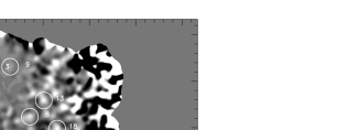
Figure 14: The $\rm 850\,\mu m$ image of the Lockman Hole field from the Hawaii Flanking Fields Survey, smoothed with a beam-size Gaussian (14.5 arcsec FWHM). The numbered circles highlight those sources found at a significance of $>3.00$. The labelling corresponds to the numbers in Table 11.

Figure 15: The $\rm 850\,\mu m$ image of the SSA13 field from the Hawaii Flanking Fields Survey, smoothed with a beam-size Gaussian (14.5 arcsec FWHM). The numbered circles highlight those sources found at a significance of $>3.00$. The labelling corresponds to the numbers in Table 12.

Figure 16: The $\rm 850\,\mu m$ image of the SSA17 field from the Hawaii Flanking Fields Survey, smoothed with a beam-size Gaussian (14.5 arcsec FWHM). The numbered circles highlight those sources found at a significance of $>3.00$. The labelling corresponds to the numbers in Table 13.

Figure 17: The $\rm 850\,\mu m$ image of the SSA22 field from the Hawaii Flanking Fields Survey, smoothed with a beam-size Gaussian (14.5 arcsec FWHM). The numbered circles highlight those sources found at a significance of $>3.00$. The labelling corresponds to the numbers in Table 14.

The “Hawaii Flanking Fields Survey (HFFS)” (Barger et al. 1998, Barger, Cowie & Sanders 1999, Barger, Cowie & Richards 2000), covers a total of $\simeq 110$  sq. arcmin over 4 regions of sky. The Lockman Hole deep field is a small pencil beam map (Barger et al. 1998), covering $\simeq 8$  sq. arcmin of sky to an rms noise level of $\rm\sigma_{850}=0.8\,mJy/beam$. The SSA13 field is composed of a deep pencil beam area ($\simeq 8$  sq. arcmin in size, $\rm\sigma_{850}=0.7$ mJy/beam; Barger et al. 1998), embedded in a wider-area, shallower map covering an additional 45 sq. arcmin with a typical rms noise level of $\rm\sigma_{850}=2.5$ mJy/beam (Barger, Cowie & Sanders 1999). The SSA17 and SSA22 fields (Barger, Cowie & Sanders 1999) both have regions of uniform noise covering approximately 20 sq. arcmin of sky, the SSA17 field to $\rm\sigma_{850}=1.6$ mJy/beam, and the SSA22 field to $\rm\sigma_{850}=0.9$ mJy/beam.

The data were originally reduced using the standard SURF pipeline, and source extraction was carried out by convolving the signal maps with the beam. In order to determine the absolute noise levels, Barger, Cowie & Sanders (1999) first eliminated any significant sources (estimated to be at the $\rm\geq 2.8\sigma$ level) by subtracting appropriately normalised versions of the beam profile. They then placed beam-sized apertures at random positions on the residual signal map, using the standard deviation between the enclosed pixels to estimate the noise. These values were then used to iteratively adjust the normalization of the variance array values, until the dispersion of the signal-to-noise ratio was approximately one.

Comparative source lists for detections with $\rm S/N>3.00$ from the two different reductions and source extraction procedures are given in Tables 11 - 14 (see also Figs 14 - 17). Columns 1-6, 8 and 9 are analogous to those of Tables 7 to 10.

In one case, a source previously identified by Barger, Cowie & Sanders (1999) has been marked with ‘bad bol.’ as this region appears to have been observed with a bad bolometer, hence the “source” is most likely to be an artefact of SURF’s attempt to interpolate between neighbouring areas of good quality data. Column 7 gives any previous reference to the $\rm 850\,\mu m$ source. Reference B99 is an abbreviation for Barger, Cowie & Sanders (1999).

The two reduction and source-extraction algorithms again produce quite different results. There is no clear trend in the variations between the independent measurements of signal-to-noise for those sources detected significantly in both analyses; in some cases the SURF reduction yields a higher signal-to-noise estimate whereas for other sources the situation is reversed. The IDL-based reduction and maximum likelihood algorithm has identified nearly twice as many peaks at the $\rm>3.00\sigma$ level as the original catalogue of Barger, Cowie & Sanders (1999), including all of their original $\rm>4.00\sigma$ objects. The comparative results for the Lockman Hole deep field given in Table 11 show that of the two sources published in Barger, Cowie & Sanders (1999), their most significant source is confirmed at $>6\sigma$. The most discrepant of the fields is the SSA13 field (Table 12), which has particulaly uneven noise when compared to all of the other survey fields and it is most likely because of this that only 4/9 of the original detections could be identified at $\rm S/N>3.00$. In the deep part of the SSA13 field, the top two sources are confirmed at better than $\rm 5.00\sigma$ in this analysis. However, in the wider shallower area only one further source listed in Barger, Cowie & Sanders (1999) could be confirmed at $\rm S/N>4.00$. Our re-analysis of the SSA17 field (Table 13) found only one of the original sources with $\rm S/N>3.50$ and with only 3/5 of the objects listed in Barger, Cowie & Sanders at $\rm>3.00\sigma$. In the SSA22 field, all 5 of the $\rm>3.00\sigma$ detected by Barger, Cowie & Sanders (1999) are recovered, with firm agreement on the top 2 sources at better than $\rm 4.00\sigma$ in both catalogues.

5.4 The Hubble Deep Field Submillimetre Survey

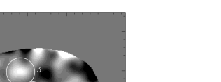
Figure 18: The $\rm 850\,\mu m$ image of the Hubble Deep Field North, smoothed with a beam-size Gaussian (14.5 arcsec FWHM). The numbered circles highlight those sources found at a significance of $>3.00$. The labelling corresponds to the numbers in Table 15.

The Hubble Deep field is the deepest of the submillimetre surveys, covering approximately 6 sq. arcmin of sky down to the confusion level of $\rm\sigma_{850}=0.5$ mJy/beam. It differs slightly from the other SCUBA surveys in that two different chop throws of 30” and 45”, both fixed in celestial coordinates, were applied to the observations, each for approximately half of the integration time. Both SURF and IDL reductions have previously been carried out on this field (Hughes et al. 1998 and Serjeant et al. 2003 respectively), but the maximum-likelihood simultaneous-fitting algorithm has not been used previously.

Comparative source lists for detections with $\rm S/N>3.00$ from the three different reductions and source extraction procedures are given in Table 15 (see also Fig 18). Column 1 gives the source number corresponding to the labelling on Fig. 18, in order of decreasing signal-to-noise. Columns 2 and 3 give the right ascension and declination of the source in J2000 coordinates. Column 4 gives the simultaneously fitted $\rm 850\,\mu m$ flux densities of the sources. The error includes a 10% calibration error combined in quadrature. Column 5 gives the measured signal-to-noise ratio of the source from the simultaneously fitted model. Column 6 defines the noise region in which the source was found; ‘central’ corresponds to the parts of the map which have seen the full integration time (outside of the deep area), and ‘edge’ corresponds to the rather noisier regions near the perimeter which have not seen the full integration time. Column 7 gives any previous reference to the $\rm 850\,\mu m$ source. Reference H98 is an abbreviation for Hughes et al. (1998), and Serj03 is an abbreviation for Serjeant et al. (2003). The presence of a * indicates that Hughes et al. (1998) deconvolved two sources here, whereas Serjeant et al. (2003) and my own reduction extracted only one. Column 8 gives the previously recorded signal-to-noise ratio where applicable, and column 9 gives the distance between the listed and previously referenced positions. The table listings given in italics correspond to previously referenced sources with $\rm S/N>3.00$, which did not meet this criteria in this analysis.

The analysis of Serjeant et al. (2003) combined the deep jigglemap imaging of the Hubble Deep Field North with additional photometry which both increased the map size slightly and improved the sampling at some positions around the edges. Since photometry measurements require pre-selection of a known object’s position this would bias the number of sources recovered in this region of sky and so this data has not been included in the analysis presented here. Consequently the sources labelled as HDF.6 and HDF.7 presented in Serjeant et al. (2003) which do not peak within the main jigglemap imaging have not been re-identified in this analysis although they have been recovered in the “HDF-N Supermap” of Borys et al. (2003). However, two new sources which have eluded previous analyses, have been recovered at the $\rm S/N>3.50$ level and all of the original detections, with the exception of HDF.3 in the Hughes et al. (1998) analysis, have been confirmed with $\rm S/N>4.00$.

6 Source Counts

Flux density	Raw 850 ${\rm\mu m}$ source counts	Corrected 850 ${\rm\mu m}$ source counts
/mJy	$N(>S)\mathrm{deg^{-2}}$	$N(>S)\mathrm{deg^{-2}}$
12.0	$2880\pm 310$	$3920^{+\phantom{0}550}_{-1120}$
12.5	$1680\pm 180$	$2140^{+\phantom{0}320}_{-\phantom{0}620}$
13.0	$1080\pm 120$	$1250^{+\phantom{0}200}_{-\phantom{0}370}$
13.5	$\phantom{0}830\pm 100$	$\phantom{0}680^{+\phantom{0}120}_{-\phantom{0}200}$
14.0	$\phantom{0}700\pm\phantom{0}90$	$\phantom{0}620^{+\phantom{0}110}_{-\phantom{0}190}$
14.5	$\phantom{0}700\pm\phantom{0}90$	$\phantom{0}490^{+\phantom{00}90}_{-\phantom{0}150}$
15.0	$\phantom{0}540\pm\phantom{0}70$	$\phantom{0}380^{+\phantom{00}70}_{-\phantom{0}120}$
15.5	$\phantom{0}500\pm\phantom{0}70$	$\phantom{0}330^{+\phantom{00}70}_{-\phantom{0}110}$
16.0	$\phantom{0}420\pm\phantom{0}60$	$\phantom{0}310^{+\phantom{00}60}_{-\phantom{0}100}$
16.5	$\phantom{0}340\pm\phantom{0}60$	$\phantom{0}230^{+\phantom{00}50}_{-\phantom{00}80}$
17.0	$\phantom{0}300\pm\phantom{0}50$	$\phantom{0}180^{+\phantom{00}50}_{-\phantom{00}60}$
17.5	$\phantom{0}260\pm\phantom{0}50$	$\phantom{0}180^{+\phantom{00}50}_{-\phantom{00}60}$
18.0	$\phantom{0}210\pm\phantom{0}40$	$\phantom{0}150^{+\phantom{00}40}_{-\phantom{00}60}$
18.5	$\phantom{0}160\pm\phantom{0}40$	$\phantom{0}100^{+\phantom{00}30}_{-\phantom{00}40}$
19.0	$\phantom{0}130\pm\phantom{0}30$	$\phantom{00}70^{+\phantom{00}30}_{-\phantom{00}30}$
19.5	$\phantom{00}90\pm\phantom{0}30$	$\phantom{00}60^{+\phantom{00}30}_{-\phantom{00}30}$
10.0	$\phantom{00}70\pm\phantom{0}20$	$\phantom{00}40^{+\phantom{00}20}_{-\phantom{00}20}$
10.5	$\phantom{00}60\pm\phantom{0}20$	$\phantom{00}20^{+\phantom{00}10}_{-\phantom{00}10}$
11.0	$\phantom{00}30\pm\phantom{0}20$	$\phantom{00}10^{+\phantom{00}10}_{-\phantom{00}10}$
11.5	$\phantom{00}20\pm\phantom{0}10$	$\phantom{00}10^{+\phantom{00}10}_{-\phantom{00}10}$
12.0	$\phantom{00}20\pm\phantom{0}10$	$\phantom{00}10^{+\phantom{00}10}_{-\phantom{00}10}$
12.5	$\phantom{00}10\pm\phantom{0}10$	$\phantom{00}10^{+\phantom{00}10}_{-\phantom{00}10}$

Table 16: The 850 ${\rm\mu m}$ source counts per square degree based on sources with S/N $>3.50$ in both survey maps, and excluding those detected in the non-uniform noise regions. Column 1 gives the flux density and column 2 the cumulative raw counts per square degree with the Poisson error. Column 3 gives the cumulative corrected counts per square degree, the upper error corresponding to the Poisson error, and the lower error accounting for both the Poisson error and the presence of spurious sources based on the simulation data.

Previous measurements of the cumulative number counts have differed quite markedly between the various surveys (eg. Blain et al. 1999, Barger, Cowie & Sanders 1999, Eales et al. 2000, Scott et al. 2002), particularly at bright flux densities ($\rm>5\,mJy$). This is not surprising given the small area of sky observed by each individual survey and the low number density of bright sources. In addition to cosmic variance, if the SCUBA sources have a tendency to cluster on scales of a few arcminutes (for which evidence is given in the next section) the problem is further compounded since it is more likely that a mapping a blank field of only several tens of square arcminutes in size will fall in an area of lower source density. Here, the sources detected with a signal-to-noise ratio $>3.50$ from our reanalysis of the CUDSS, Hawaii and HDF surveys have been combined with those identified in the 8 mJy Survey, to produce the most accurate number counts to date, from $2-12.5$ mJy at 0.5 mJy intervals. The regions of non-uniform noise towards the edge of the maps and any sources they contained were excluded. The simulations described in Section 4.1 were used to correct for the effects of flux-density boosting and incompleteness on a field by field basis. Estimating the level of contamination from spurious / confused sources, however, requires the generation of fully simulated images. The accuracy of such images is hampered by the lack of knowledge regarding the clustering properties of the SCUBA population down to the faintest flux density levels. The simulations described in Section 4.2 imply that the fraction of spurious / confused sources (defined as having no input source at least half as bright as the output flux density) at a significance of $\rm>3.50\sigma$ is $\simeq 30\%$. This number is in line with the upper limit placed on the confused / spurious fraction from deep radio follow-up of the “8 mJy Survey” fields (Ivison et al. 2002). The raw and corrected cumulative number counts are given in Table 16 along with $\rm 1\sigma$ Poisson error bars (calculated from the square root of the number of detections on which the source count was based). The estimated 30% fraction of spurious / confused sources has been combined in quadrature with the lower Poisson error bar in the corrected number counts.

Figure 19: Cumulative number counts corrected for the effects of boosting and incompleteness versus the raw number counts. The dotted line marks the case where the raw and corrected cumulative numbers counts are the same. The error bars are as given in Table 16.

Figure 20: A plot of differential number counts vs. flux density. The solid diamonds represent data from the combined blank field survey re-analysis only, with $\rm 1\sigma$ Poisson error bars on the y-axis, and the flux density range on which the differential count is based marked as an error bar on the x-axis. The open triangles represent data points from the lensing surveys of Blain et al. (1999) and Cowie et al. (2002). The solid curve is a best fit parametric model of the form $\rm n(s)=\frac{N_{0}}{(a+S^{\alpha})}$.

Figure 19 shows the corrected versus the raw number counts at each flux density, together with a dotted line marking the locus of where the raw and corrected counts take the same value. An increase in the cumulative number counts along either axis correponds to a decrease in the flux density threshold. One can see immediately that at brighter flux densities, the effect of boosting is stronger than incompleteness and hence the real number density of sources above a specified flux density threshold is lower than the directly measured value. This may also be implied from an examination of the raw data alone. The area of sky mapped in the “SCUBA 8 mJy Survey” is almost identical to the area of sky mapped by the other deeper surveys combined. At bright flux densities the deeper surveys are essentially complete and so one can compare the number of detections above a specified signal-to-noise ratio and flux density threshold between the shallower and deeper maps. For a retrieved $\rm S_{850\mu m}>10\,mJy$ and $\rm S/N>3.50$, the “SCUBA 8 mJy Survey” identified 8 sources, whereas in all the other surveys only 1 source was found to satisfy this criteria. Similarly, for a retrieved $\rm S_{850\mu m}>8\,mJy$ and $\rm S/N>3.50$, the “SCUBA 8 mJy Survey” identified 20 objects, whereas only a total of 5 were found in the other surveys. Given the small area of sky considered, part of the discrepancy between the number of bright sources recovered in the “SCUBA 8 mJy Survey” and the other deeper blank field surveys can be explained by small number statistics but it seems highly unlikely that this is the sole cause. Moving towards fainter flux density thresholds, the increased source density makes incompleteness more of a problem and around the confusion limit of $\rm\sim 3\,mJy$ (where the density of sources is $\simeq 1000$ per square degree) the raw and corrected cumulative number counts are approximately the same.

One of the simplest ways of describing the number counts is by carrying out a simple parametric fit of a power-law model to the differential number counts as a function of flux density. The differential number counts at a specific flux density were determined by the difference in cumulative counts between the two values on either side of the data point, divided by the change in flux density, which approximates to a measure of the gradient of a tangent to the cumulative number counts curve at that point. The completeness and boosting corrected number counts were used for this procedure. Following Barger, Cowie & Sanders (1999), a model of the form

$$\rm n(S)=\frac{dN(S)}{dS}=\frac{N_{0}}{(a+S^{\alpha})}$$ (13)

was fitted to the differential data points by means of a minimised $\rm\chi^{2}$ method, where the values of $\rm N_{0}$, a and $\rm\alpha$ were allowed to vary freely. The best fit values for these parameters were $\rm N_{0}=2.67\times 10^{4}$, $\rm a=0.49$ and $\rm\alpha=3.14$, predicting a total $\rm 850\,\mu m$ background of $\rm 3.8\times 10^{4}\,mJy\,deg^{-2}$, mid-way between the $\rm 850\,\mu m$ extragalactic values of $\rm 3.1\times 10^{4}\,mJy\,deg^{-2}$ and $\rm 4.4\times 10^{4}\,mJy\,deg^{-2}$ as measured from COBE-FIRAS by Puget et al. (1996) and Fixsen et al. (1998) for the lower and upper values respectively. The values of the fitted parameters are in fact very close to the values originally determined by Barger, Cowie & Sanders (1999) who found $\rm N_{0}=3.0\times 10^{4}$, $\rm a=0.5$ and $\rm\alpha=3.2$. Figure 20 shows a plot of the differential number counts against flux density. The solid diamonds represent data from the combined blank field survey re-analysis only, with $\rm 1\sigma$ Poisson error bars on the y-axis and a flux density range of 1 mJy on the x-axis, corresponding to the change in flux density between the two data points on either side of the point at which the differential counts has been determined. The open triangles represent data points from the lensing surveys of Blain et al. 1999 and Cowie et al. 2002, and the solid curve is the best fit parametric model.

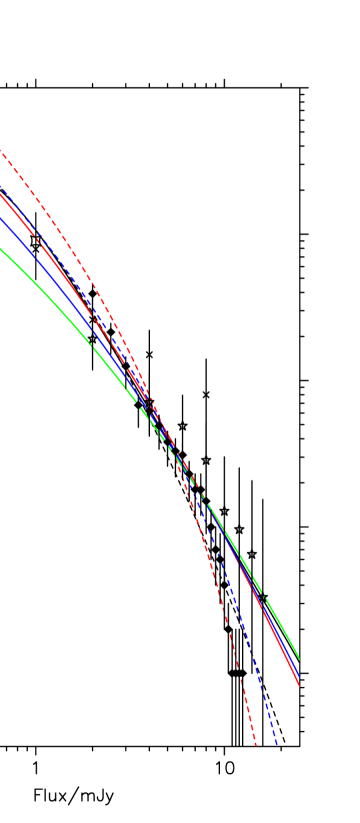
Figure 21: A plot of cumulative number counts vs. flux density, along with a series of models assuming an $\rm\Omega_{M}=0.3$, $\rm\Omega_{\Lambda}=0.7$ cosmology. The solid diamonds represent the cumulative source counts from the completeness and boosting corrected counts derived from the combined blank field survey re-analysis only, with error bars as given in Table 16. The crosses and round-edged squares represent data points from the lensing surveys of Blain et al. (1999) and Cowie et al. (2002) respectively, while the stars indicate the results of and Borys et al. (2003). The various models are described in the main text.

Fig. 21 shows the corrected cumulative number counts, as well as a series of models predicting the $\rm 850\,\mu m$ source counts for an adopted $\rm\Omega_{M}=0.3$, $\rm\Omega_{\Lambda}=0.7$ cosmology, in line with the most recent cosmological parameter results from the supernova cosmology project (Perlmutter et al. 1999), X-ray clusters (Allen, Schmidt & Fabian 2002a, 2002b), and WMAP observations of the cosmic microwave background (Spergel et al. 2003). A value of $\rm H_{0}=67\,km\,s^{-1}\,Mpc^{-1}$ was assumed throughout. The black lines are parameterised models, the solid lines following a simple power-law description of the data points and are the same for both figures. The dashed lines represent work by Rowan-Robinson (2000,2001) who generated best-fit models of the measured far-infrared through to submillimetre number counts, as constrained by the extragalactic background, for a number of assumed cosmologies. In the remaining models (red, blue and green curves), values of dust temperature $\rm T_{d}$ and emissivity index $\rm\beta$ based on optically thin greybody emission, were allowed to vary where necessary so that as good a fit as possible could be obtained for the $\rm\Omega_{M}=0.3$, $\rm\Omega_{\Lambda}=0.7$ cosmology.

The solid black line is the integrated $\rm dN/dS$ best-fit parametric model given in equation 13, providing a good description of the cumulative number counts for $\rm S_{850}<10\,mJy$. Rowan-Robinson (2001) has also taken a parameterised approach to modelling the infrared through to submillimetre counts and backgrounds, in this case by using multiwavelength observational data in these wavelength regimes to place constraints on models made up of four spectral components: infrared cirrus, an M82-like starburst, an Arp220-like starburst and an AGN torus. The model assumes that the evolution of the star formation rate manifests itself as pure luminosity evolution. The models, consistent with infrared and submillimetre counts and backgrounds, showed a flat star formation rate from $z=1-3$, in agreement with other studies of the star formation history such as the HDF (Hughes et al. 1998). The most striking difference between other modelling work and Rowan-Robinson (2001) is the dominant role of the cirrus component at submillimetre wavelengths. The black dashed line in Fig. 21 shows the model of Rowan-Robinson (2001) which appears to be the best-fit of those presented here to the cumulative $\rm 850\,\mu m$ source count data points over the whole flux density range.

The red lines on Fig. 21 represent a pure luminosity evolution of the form $(1+z)^{3}$ out to a threshold redshift, and constant thereafter. The solid line began with the $\rm 60\,\mu m$ luminosity function of Saunders et al. (1990), interpolated to $\rm 850\,\mu m$ assuming an optically thin greybody with a single dust temperature and emissivity index, to describe the far-infrared / submm dust SED. The same values for $\rm T_{d}$ and $\rm\beta$ were assumed in calculating the K-correction for consistency. The dashed line began with the $\rm 850\,\mu m$ luminosity function measured by Dunne et al. (2000). A dust temperature of $\rm 40\,K$ and emissivity index of $\rm\beta=1.3$ appeared to best satisfy the data points, using threshold redshifts of $z=2.0$ and $z=1.5$ for the Saunders et al. (1990) and Dunne et al. (2000) based luminosity functions respectively. This simple description of luminosity evolution appeared to work well for the interpolated Saunders et al. (1990) $\rm 60\,\mu m$ luminosity function for $\rm S_{850}<8\,mJy$, but predicted too many sources brighter than this. Conversely, using the Dunne et al. (2000) $\rm 850\,\mu m$ luminosity function, a good fit to the data points was found for $\rm S_{850}>2\,mJy$ but overpredicted the number of sources fainter than this by a factor of 2-3.

The solid and dashed blue lines on the cumulative number density plot also assume pure luminosity evolution of the interpolated $\rm 60\,\mu m$ Saunders et al. (1990) and directly measured $\rm 850\,\mu m$ Dunne et al. (2000) luminosity functions respectively. In this case, however, the luminosity evolution $\rm g(\mathit{z})$ takes a more realistic form, which is fully compatible with models of cosmic chemical evolution and naturally includes a peak in the evolution function (Jameson et al. 1999, Smail et al. 2002):

$$\rm g(\mathit{z})=(1+\mathit{z})\rm^{3/2}sech^{2}[bln(1+\mathit{z})\rm-c]cosh^{2}c$$ (14)

where best fits values for the parameters b and c based on multiwavelength far-infrared to submillimetre counts and constraints on the probable redshift distribution of the $\rm 850\,\mu m$ population (Smail et al. 2002) are $\rm b=2.2\pm 0.1$ and $\rm c=1.84\pm 0.1$. The interpolated $\rm 60\,\mu m$ luminosity function combined with this description of pure luminosity evolution fits the data well for $\rm S_{850}<8\,mJy$ assuming an optically thin greybody description of the thermal dust emission with parameters $\rm T_{d}=39\,K$ and $\rm\beta=1.3$. The data points across the whole flux density range are fitted well using the Dunne et al. (2000) $\rm 850\,\mu m$ luminosity function assuming dust emission parameters of $\rm T_{d}=30\,K$ and $\rm\beta=1.0$, although it should be noted that this combination of dust temperature and emissivity index does not describe the spectral energy distribution well for any known local galaxies based on the “SCUBA Local Universe Galaxy Survey (SLUGS)” (Dunne et al. 2000).

The solid green line on Fig. 21 uses the $\rm 60\,\mu m$ luminosity function of Saunders et al. (1990) combined with luminosity evolution taking the form $(1+z)^{4}$ up to a threshold redshift $z_{\mathrm{thresh}}$, and $(1+z)^{-4}$ thereafter (Chapman et al. 2002a). They find a best fit of $z_{\mathrm{thresh}}=2.6$ for the transitional redshift, based on current constraints on the redshift distribution as well as the source counts. This particular $\rm 850\,\mu m$ counts model has a rather shallower gradient than the others and could only be made to match number counts of this combined re-analysis over the flux density range $\rm\sim 3-7\,mJy$ for $\rm T_{d}=36\,K$ and a very extreme $\rm\beta=2.0$. Possibly a higher value of the dust emissivity index could produce a steeper counts model, however, such high values are not observed in in any known class of objects. No satisfactory fit could be obtained beginning with the Dunne et al. (2000) $\rm 850\,\mu m$ luminosity function. The proposed Chapman et al. (2002a) luminosity evolution does not seem consistent with the blank field survey source counts, although the number counts derived from the lensing survey of Blain et al. 1999 are much shallower, predicting rather higher number densities of bright sources, and could plausibly be fit by this scenario for less extreme values of $\rm beta$.

One particularly interesting feature of this source counts re-analysis is the apparent steepening of the cumulative number counts beyond $\rm S_{850}>8\,mJy$. This could at least in part be due to small number statistics of the brightest sources, however, if real has some important implications. Firstly, it could indicate an intrinsic turn-over in the underlying luminosity function. In turn, this would suggest a very interesting upper limit on the luminosity of a high redshift galaxy, perhaps reflecting an upper limit on the overall mass of the system. This could place useful constraints on galaxy formation theories. Secondly, a steepening of the bright source counts could make the SCUBA population much more prone to the effects of gravitational lensing. For weak lensing scenarios, the ratio of the number of observed sources brighter than a flux density threshold to the true number of sources brighter than that flux density threshold is given by

$$\rm\frac{N_{obs}(>S)}{N_{true}(>S)}=\mu^{\gamma-1}$$ (15)

where $\rm\mu$ is the magnification amplitude and $\gamma$ is the slope of the cumulative source counts. For $\rm 1<S_{850}<8\,mJy$ the counts slope $\rm\gamma\simeq 2.5$, whereas for $\rm S_{850}>8\,mJy$ this increases to $\rm\gamma\simeq 5.5$. No attempt has been made to correct the $\rm 850\,\mu m$ source counts for the effects of lensing, but there is some evidence to suggest that some blank field sources have been gravitationally lensed. Almaini et al. (2003) found a strong cross-correlation in the ELAIS N2 field between the distribution of SCUBA and Chandra sources even though the coincidence of detections in the submillimetre and X-ray wavelengths was only $\sim 5\%$. One proposed explanation for this effect is that the SCUBA and Chandra sources trace the same large scale structure at high redshift ($z>1$), however, there also appears to be a similarly strong cross-correlation between the low redshift $I-$band sources and the higher redshift SCUBA and Chandra sources in this field (Almaini et al. 2005) suggesting an alternative explanation may be valid: the SCUBA and Chandra detections may have been magnified in certain regions of the field by the presence of high mass density structure, as traced by the $I-$band imaging, at $z\simeq 0.5$. Chapman et al. (2002b) have also pointed out that some submillimetre sources have apparent counterparts which are optically bright galaxies, $I<21.5$, lying at modest redshifts, $z<1$. This could of course be explained by these counterparts being correct, reflecting a population of galaxies which are detected as very cold, luminous submillimetre sources, however, a second explanation for such systems is that the optically bright galaxy is a foreground object acting as a gravitational lens, amplifying the more distant SCUBA galaxy. The detection of luminous molecular CO emission at the redshift of the optically bright galaxy would provide a powerful test to distinguish between these two scenarios. If the latter explanation of gravitational lensing is correct, Chapman et al. (2002b) estimate that up to $\rm 3-5\%$ of the $>10$ mJy submillimetre sources detected in blank field surveys could be gravitationally amplified by foreground galaxies.

Gravitational lensing by clusters of galaxies can of course be used to study the fainter submillimetre sources, and this technique has been successfully applied by Blain et al. (1999) and Cowie et al. (2002) (the data points marked by the crosses and curved-edged squares on Fig. 21 respectively). The agreement between the source counts derived from the two cluster-lensing surveys is extremely good at flux densities below $\rm S_{850}\simeq 2$ mJy, and there is a smooth transition at this point between the faint number counts from the cluster-lensing surveys and the brighter source counts from our combined reanalysis of the blank field surveys. However, the number counts derived by Blain et al. (1999) at 4 and 8 mJy are significantly higher than the combined blank field survey counts presented in Table 16. The most likely explanation for this discrepancy is that the numbers quoted by Blain et al. (1999) suffer badly from small number statistics at bright flux densities, their lensing survey being composed of a number of small fields covering a total area of sky of only a few tens of square arcminutes. In comparison, the total area of sky observed by the “8 mJy Survey”, “CUDSS”, “HDF” and “Hawaii Survey” is 460 sq. arcmin, an order of magnitude larger. If the bright SCUBA population does strongly cluster on arcminute scales, as implied by the evidence presented in Section 7, this could also affect the bright end of the number counts in small area surveys such as Blain et al. (1999).

The data points marked on Fig. 21 by open stars are determined from the 165 sq. arcmin “Hubble Deep Field North SCUBA Super-map” presented by Borys et al. (2003). The rms noise level of of this composite map ranges from $\rm\sigma_{rms}\simeq 0.5-7$ mJy / beam (Borys et al. 2003). In general the counts of Borys et al. (2003) are slightly higher than those determined from this re-analysis, although they agree to well within the error bars for $\rm S_{850}<10\,mJy$. At brighter flux densities, the two sets of cumulative number counts begin to diverge, those of Borys et al. (2003) continuing to follow an approximately power-law decline with increasing flux density whereas those presented in this paper steepen quite markedly. There are several possible reasons for this discrepancy. Firstly both of these analyses suffer from small number statistics at the brightest flux densities ($\rm S_{850}>10\,mJy$) and so cosmic variance may be an issue particularly if these objects tend to cluster on arcminute scales. Secondly Borys et al. had problems calibrating their wide area scan-map data which represents the shallowest regions of the super-map. If they have over-estimated their flux conversion factors by $\rm\sim 20\%$ the two sets of number count measurements agree well. Finally 4/5 of the sources recovered by Borys et al. at $\rm S/N>3.5$ and $\rm S_{850}>16\,mJy$ have rms noise levels of $\rm\sigma_{rms}>5$ mJy/beam suggesting that these may have been recovered in non-uniform edge regions for which the simulations presented in section 4.2 have shown to have very poor source reliability. This would obviously increase the cumulative number count measurements at all flux densities fainter than this.

Overall, the increased accuracy of this new source counts analysis will allow the evolutionary nature, as well as the dust and star-forming properties of the submillimetre population to be studied in much more detail than has been possible before. This will be particularly useful when combined with knowledge of the redshift distribution of submillimetre sources, which is slowly being built up at the present.

7 Clustering

If the bright 850 $\rm\mu m$ sources are indeed the progenitors of massive elliptical galaxies then they should be strongly clustered, an inevitable result of gravitational collapse from Gaussian initial density fluctuations since the rare high-mass peaks are strongly biased with respect to the mass. There is a great deal of evidence to support the presence of this bias at high redshift. The correlations of Lyman-break galaxies at $z\simeq 3$ (Steidel et al. 1999) are almost identical to those of present-day field galaxies, even though the mass must have been much more uniform at early times. Furthermore, the correlations increase with UV luminosity (Giavalisco & Dickinson 2001) reaching scale lengths of $r_{0}\simeq 7.5h^{-1}$ Mpc - approximately 1.5 times the present-day value. In the case of luminous proto-ellipticals an even stronger bias is expected since one is selecting not just massive galaxies but those that have collapsed particularly early in order to generate the oldest stellar populations. This is suggested by studies of the local Universe which have shown that early-type galaxies are much more clustered than late-type galaxies (eg. Guzzo et al. 1997, Willmer et al. 1998), and more recently by the findings of Daddi et al. (2000) who have investigated the clustering properties of extremely red objects (EROs). They detect a strong clustering signal of the EROs which is about an order of magnitude larger than the clustering of $K-$selected field galaxies, and also report a smooth trend of increasing clustering amplitude with increasing $R-K$ colour, reaching $r_{0}\simeq 11h^{-1}$ Mpc for $R-K>5$. These results are probably the strongest evidence to date that the largest fraction of EROs is composed of ellipticals at $z>1$. There are already some hints of strong clustering in the bright sub-mm population from the discovery of a strong excess of bright SCUBA sources around high-redshift AGN (Ivison et al. 2000, Stevens et al. 2003). Blain et al. (2004) have also combined a sample of 73 submillimetre galaxies over seven fields for which they had spectroscopic redshifts, finding tentative evidence for strong clustering of submillimetre galaxies with a correlation length $r_{0}\sim(6.9\pm 2.1)h^{-1}$ Mpc.

7.1 Angular correlation functions

The angular correlation function $\rm w(\theta)$ is the projection of the spatial function on the sky and is defined in terms of the joint probability $\rm\delta P$ of finding two galaxies separated by an angular distance $\rm\theta$ with respect to that expected for a random distribution

$$\rm\delta P=N^{2}[1+w(\theta)]\delta\Omega_{1}\delta\Omega_{2}$$ (16)

where $\rm\delta\Omega_{1}$ and $\rm\delta\Omega_{2}$ are elements of solid angle, and $\rm N$ is the mean surface density of objects. If $\rm w(\theta)=0$ the distribution is homgeneous. A positive $\rm w(\theta)$, therefore, corresponds to an over-density of sources separated by distance $\rm\theta$.

There are a variety of possible estimators for $w(\theta)$ as a function of pair-count ratios. Following Landy & Szalay (1993), we have adopted the estimator:

$$\rm w(\theta)=\frac{(DD-2DR+RR)}{RR}$$ (17)

in which the variance is minimised to almost Poisson level. DD is the number of distinct data pairs in the real image within a bin covering a specified range of $\rm\theta$, DR is the number of cross-pairs between the real and mock catalogues within the same range of $\rm\theta$, and RR is the number of random-random pairs. DR and RR are normalised with respect to the total number of data-data pairs from the real image.

Scott et al. (2002) made the first attempt at measuring an angular correlation function for the bright SCUBA population. Their results provided tentative evidence for strong clustering of the submillimetre sources on scales of 1-2 arcmin but proved inconclusive due to the small number of sources recovered in the “8 mJy Survey” alone. More recent attempts to measure the clustering strength have relied on combining catalogues of submillimetre sources with Lyman-break galaxies (Webb et al. 2003b) or Chandra sources (Almaini et al. 2003) and assuming that even though the objects were rarely coincident, the two populations identified at different wavelengths were tracing the same large scale structure. These results further supported the view that the bright SCUBA galaxies cluster strongly on arcminute scales, however, in both cases the combined correlation functions were dominated by the larger number of Lyman-break galaxies or Chandra sources.

Further SCUBA galaxy clustering measurements, some tentatively detecting clustering, have been made (Blain et al. 2004, Borys et al. 2004, Webb et al. 2003a).

Here, the 2-point angular correlation function analysis combines the sources identified in the “8 mJy Survey” fields with those objects detected in this re-reduction of the other blank field surveys, effectively creating a master catalogue with sources from double the area of the “8 mJy Survey” alone.

A catalogue of randomly placed fake sources was created for each of the survey fields, with the number of fake objects contained in each field’s random catalogue chosen to be directly proportional to the area of the image (number in mock catalogue $\rm=0.01\times Area(/arcsec^{2})$), so as to reflect a uniform number density across the sky. The wider area fields which dominate this analysis are largely signal-to-noise limited even at bright flux densities, and hence there is an increasing probability of finding significant detections in deeper regions of the maps. Although the positions were allocated randomly, the Gaussian convolved noise maps were used to weight the number density of sources across the image, since a larger density of sources above a specified signal-to-noise threshold would be expected in regions of lower noise. In practice, this meant dividing the full image into a series of sub-images, 20 arcsec by 20 arcsec in size, and calculating the mean noise level in each of these grid sections. For sources brighter than $\rm\simeq 5\,mJy$, the number of sources expected above a constant signal-to-noise threshold increases approximately as $\rm N(>S_{850\mu m})\propto S_{850\mu m}^{-1.5}$, and consequently the relative number of sources in each sub-image scales as $\langle\mathrm{noise}\rangle^{-1.5}$. The fake source positions were then allocated according to a Poisson distribution, masking any positions which were covered by a negative sidelobe accompanying a significant source in the real survey data. If the number of fake sources included in the catalogue is very much larger than the number recovered from the real data (as is the case here), this is in essence equivalent to choosing positions by combining the results from source extraction on a series of fully simulated survey fields. Detections lying in non-uniform regions of the maps in both the real and fake catalogues were omitted from the correlation function calculations since many of the objects recovered in the real data in these high noise regions were likely to be spurious (see Section 4.2).

Although combining all existing blank field survey data together does increase the number of sources on which a correlation function can be based, the numbers are still fairly small. Above a signal-to-noise ratio of 3.50, there are a total of 53 sources detected brighter than 5 mJy, of which 51 may be used in a correlation function analysis (the other 2 are lone sources in two of the deep single SCUBA pointing fields). This number increases to 104 sources brighter than 5 mJy at $\rm>3.00\sigma$, of which 100 may be used in a correlation function analysis. However, this will also increase the contribution from spurious sources in the catalogue and may therefore dilute the measured signal. Figs. 22 and 23 show the directly measured angular correlation data points for detections brighter than 5 mJy, with $\rm 1\sigma$ Poisson error bars, and for signal-to-noise thresholds of $>3.50$ and $>3.00$ respectively. The bin-size used in both plots is 29 arcsec (twice the beam-size). Rather surprisingly, there is little change in

Figure 22: 2-point angular correlation function for sources brighter than 5 mJy, detected at a significance of $\rm>3.50\sigma$, over all of the survey fields. The error bars are $\rm 1\sigma$ Poisson errors. The solid power-law line indicates the correlation function found by Daddi et al. (2000) for EROs with $R-K>5$ and $K<18.5$, and the dashed power-law line indicates the correlation function found by Giavalisco et al. (1998) for Lyman break galaxies at $z\sim 3$. The dot-dash line shows the best-fit power-law to the data points. The vertical dotted line indicates the size of the JCMT beam at $\rm 850\,\mu m$.

Figure 23: 2-point angular correlation function for sources brighter than 5 mJy, detected at a significance of $\rm>3.00\sigma$, over all of the survey fields. The error bars are $\rm 1\sigma$ Poisson errors. The solid power-law line indicates the correlation function found by Daddi et al. (2000) for EROs with $R-K>5$ and $K<18.5$, and the dashed power-law line indicates the correlation function found by Giavalisco et al. (1998) for Lyman break galaxies at $z\sim 3$. The dot-dash line shows the best-fit power-law to the data points. The vertical dotted line indicates the size of the JCMT beam at $\rm 850\,\mu m$.

Figure 24: 2-point angular correlation function for sources brighter than 6 mJy, detected at a significance of $\rm>3.00\sigma$, over all of the survey fields. The error bars are $\rm 1\sigma$ Poisson errors. The solid power-law line indicates the correlation function found by Daddi et al. (2000) for EROs with $R-K>5$ and $K<18.5$, and the dashed power-law line indicates the correlation function found by Giavalisco et al. (1998) for Lyman break galaxies at $z\sim 3$. The dot-dash line shows the best-fit power-law to the data points. The vertical dotted line indicates the size of the JCMT beam at $\rm 850\,\mu m$.

Figure 25: 2-point angular correlation function for sources brighter than 7 mJy, detected at a significance of $\rm>3.00\sigma$, over all of the survey fields. The error bars are $\rm 1\sigma$ Poisson errors. The solid power-law line indicates the correlation function found by Daddi et al. (2000) for EROs with $R-K>5$ and $K<18.5$, and the dashed power-law line indicates the correlation function found by Giavalisco et al. (1998) for Lyman break galaxies at $z\sim 3$. The dot-dash line shows the best-fit power-law to the data points. The vertical dotted line indicates the size of the JCMT beam at $\rm 850\,\mu m$.

Flux density	S/N	A($\rm\theta/deg$)	$\rm\delta$	$\rm\sigma^{2}$	$\rm\theta_{0}$
threshold	threshold				/arcsec
$\rm>5\,mJy$	$>3.50$	$5.00\times 10^{-2}$	0.70	0.386	49.9
$\rm>5\,mJy$	$>3.00$	$1.82\times 10^{-2}$	0.89	0.230	39.9
$\rm>6\,mJy$	$>3.00$	$2.49\times 10^{-3}$	1.36	0.280	43.8
$\rm>7\,mJy$	$>3.00$	$1.31\times 10^{-3}$	1.56	0.265	46.7

Table 17: Best-fit parameters to the angular correlation functions shown in Figs. 22 to 25. Column 1 gives the flux density cutoff as measured from the raw images and Column 2 gives the signal-to-noise cutoff for source detection. Colum 3 gives the amplitude A, Column 4 gives the slope of the power-law $\rm\delta$, Column 5 gives the integral constraint $\rm\sigma^{2}$ and Column 6 gives the characteristic angular separation $\rm\theta_{0}$.

the proportion of excess pairs between corresponding data points in the first 100 arcsec of the two plots. The Gaussian-convolved noise images did not imply that there was anything unusual about the survey data in regions of higher than average $\rm 3.00\sigma$ source density, indicating that elevated noise where there is a concentration of significant detections is unlikely to be the cause. There are two likely explanations as to why the signal from the $\rm>3.50\sigma$ catalogue is not diluted in the $\rm>3.00\sigma$ plot. Firstly, the simulation results in Section 4.2, which made estimates of the fraction of spurious / confused sources at various signal-to-noise thresholds, have been pessimistic. It is difficult to generate accurate realisations of the SCUBA maps on which to make estimates of contamination in a source catalogue due to confusion and noise without knowing the clustering properties of the SCUBA population in the first place, and the fact that there is very little difference in the proportion of excess pairs on scales of $\sim 1$ arcmin between the two signal-to-noise datasets may be suggesting that most of the $\rm 3.00-3.49\sigma$ sources are real. Perhaps a more likely scenario, however, is that the clustering properties of the SCUBA population are strong over a significant range of flux densities, and thus detections arising from the confusion of faint objects are more likely to be found on the same scale and in the vicinity of the real bright SCUBA sources. The major difference between the $\rm>3.00$ and $\rm>3.50\sigma$ plots is the size of the Poisson error bars. As one might expect, the error bars are a factor of $\sim\sqrt{2}$ smaller in Fig. 23, reflecting the increase by a factor of 2 of the number of sources considered, increasing the significance of the number of excess pairs contained in the first 3 bins (14.5 - 101.5 arcsec) from $\rm 2.5$ to $\rm 3.7\sigma$.

Cutting at higher flux densities decreases the number of sources available for producing a 2-point angular correlation function even further, thus using the smaller “safer” catalogue of sources above a signal-to-noise threshold of 3.50 leads to tentative but non-significant measures of the clustering strength above the noise level. Instead, the analysis has been repeated using the full $\rm>3.00\sigma$ source lists for flux density cut-offs of $>6$ and $>7$ mJy shown in Figs. 24 and 25 respectively, pushing the available data to its limits. It should be noted that these flux density thresholds are the raw values as measured directly from the maps and should therefore not be taken as “absolute” because of the boosting effects described in Section 4.1. However, it is fair to say that cutting at $\rm S_{850}>7$ mJy defines a set of objects with generally higher star formation rates than cutting at $\rm S_{850}>5$ mJy and so Figs. 23 to 25 can still be used to look for any trends in clustering strength with increasing flux density. For comparison, the number of excess pairs within $\sim 100$ arcsec of each other in the real data when compared to a random distribution is significant at the $\rm 3.3\sigma$ level for $\rm S_{850\mu m}>6$ mJy, and at the $\rm 3.5\sigma$ level for $\rm S_{850\mu m}>7$ mJy.

For all three flux density limits, the measured correlation functions indicate a clustering strength much larger than that measured by Giavalisco et al. (1998) for Lyman-break galaxies at $z\simeq 3$ (the dashed lines in the figures), even given the rather large error bars on the SCUBA data points. Could the apparent difference in clustering strength simply be due to projection effects over redshift space? The Lyman-break technique uses colour selection to identify high-redshift galaxies through multi-band imaging across the $\rm 1216\AA$ line and the $\rm 912\AA$ Lyman break. At $z>2.5$ the Lyman limit is redshifted far enough into the optical window to be observable in broad-band ground-based photometry. By placing filters on either side of the redshifted Lyman limit one can find high-redshift objects by their strong spectral breaks. Giavalisco et al. (1998) used a custom photometric system, $U_{n}GR$ (Steidel & Hamilton 1993) optimized for selecting Lyman-break galaxies with $z\simeq 3$. By the nature of this method, 90% of the galaxies they used were confined to the redshift range $2.6<z<3.4$, with none at $z<2.2$. The redshift range of the bright SCUBA population used in these calculations of angular correlation functions is much more uncertain, but Ivison et al. (2002) have suggested a median redshift of $z=2.4$ based on the radio-to-submillimetre spectral indices (Carilli & Yun, 1999 & 2000), with inferred redshifts spanning the range of $z\simeq 1-4$. Therefore, unless the bright SCUBA population occupies a very much narrower redshift band than implied by the radio-to-submillimetre spectral indices the dilution of the angular clustering signal by projection over redshift cannot be the reason for the large difference in clustering strength.

Instead, this contrast in clustering properties implies that the Lyman-break galaxies and bright SCUBA sources are sampling two different stages or mass domains in galaxy formation (see also Barger, Cowie & Richards 2000, Webb et al. 2003b). The stronger clustering exhibited by the bright $\rm 850\,\mu m$ sources suggests that these objects are tracing the rarest high-mass peaks of the Gaussian initial density fluctuations and are the progenitors of the most massive ellipticals, whereas the weaker clustering of the Lyman-break galaxies indicates a weaker bias with respect to mass, detecting the formation of smaller disk or bulge systems. The strength of clustering, however, is consistent with that measured by Daddi et al. (2000) for extremely red objects (EROs) with $K<18.5$ and $R-K>5$ (the solid lines in the figures), perhaps suggesting an evolutionary sequence from SCUBA source to ERO. The numerical coincidence between the co-moving number densities of EROs and that estimated for bright SCUBA sources is also in line with this idea (Scott et al. 2002).

Attempts have been made to fit a standard power-law describing the angular correlation function to the data points shown in Figs. 22 to 25. The fit is slightly complicated by the fact that the global number density is unknown and must be estimated from the sample to hand. Hence,

$$\rm(1+w_{true}(\theta))=(1+w_{obs}(\theta))\left(\frac{\bar{n}}{<n>}\right)^{2}$$ (18)

where $\rm w(\theta)_{true}$ is the true correlation function, $\rm w(\theta)_{obs}$ is the observed correlation function, $\rm\bar{n}$ is the mean number density of sources and $\rm<n>$ is the global number density of sources. One can rewrite the observed mean number density $\rm\bar{n}$ in terms of a pertubation $\rm\delta n$ on the global number density $\rm<n>$ (ie. $\rm\bar{n}=<n>\pm\delta n$), such that in averaging over a set of sky areas the size of the sample

$$\rm(1+w_{true}(\theta))=(1+w_{obs}(\theta))(1+\sigma^{2})$$ (19)

where $\rm\sigma^{2}$ is the rms surface density variation. If the real correlation functions take the power-law form $\rm w_{true}(\theta)=A\theta^{-\delta}=\left(\frac{theta}{theta_{0}}\right)^{-delta}$, then

$$\rm w_{obs}(\theta)=\frac{(A\theta^{-\delta})-\sigma^{2}}{1+\sigma^{2}}=\frac{\left(\frac{\theta}{\theta_{0}}\right)^{-\delta}-\sigma^{2}}{1+\sigma^{2}}$$ (20)

Figure 26: Nearest-neighbour analysis for sources brighter than 5 mJy, detected at a significance of $\rm>3.00\sigma$ over all of the survey fields.The vertical dotted line indicates the size of the JCMT beam at $\rm 850\,\mu m$. The solid line shows the distribution of nearest-neighbour pairs for the actual dataset, whereas the dashed line shows the expected nearest-neighbour histogram for the same surface density of sources when distributed randomly. The probability that the two distributions are the same is $<0.05$.

Figure 27: Nearest-neighbour analysis for sources brighter than 6 mJy, detected at a significance of $\rm>3.00\sigma$ over all of the survey fields.The vertical dotted line indicates the size of the JCMT beam at $\rm 850\,\mu m$. The solid line shows the distribution of nearest-neighbour pairs for the actual dataset, whereas the dashed line shows the expected nearest-neighbour histogram for the same surface density of sources when distributed randomly. The probability that the two distributions are the same is $\rm<0.05$.

Figure 28: Nearest-neighbour analysis for sources brighter than 7 mJy, detected at a significance of $\rm>3.00\sigma$ over all of the survey fields.The vertical dotted line indicates the size of the JCMT beam at $\rm 850\,\mu m$. The solid line shows the distribution of nearest-neighbour pairs for the actual dataset, whereas the dashed line shows the expected nearest-neighbour histogram for the same surface density of sources when distributed randomly. The probability that the two distributions are the same is $\rm<0.01$.

One can then either determine the values of A, $\rm\delta$ and $\rm\sigma^{2}$ by allowing them all to be free parameters in a minimised $\rm\chi^{2}$ fit, or alternatively one can rewrite the integral constraint in terms of the amplitude multiplied by a constant (ie. $\rm\sigma^{2}=A\times C$) and estimate C by doubly integrating an assumed true $\rm w(\theta)$ over the field area $\rm\Omega$,

$$\rm AC=\frac{1}{\Omega^{2}}\int\int w(\theta)d\Omega_{1}d\Omega_{2}$$ (21)

This can be done numerically using the random-random correlation, such that

$$\rm C=\frac{\sum N_{rr}(\theta)\theta^{-\delta}}{\sum N_{rr}(\theta)}$$ (22)

Both of these methods have been attempted for all four sets of data points, the free parameter fit proving to be the more successful of the two. The results are given in Table 17.

The large error bars and scatter in the data points beyond the first 3 fairly robust data point measurements (out to $\sim 100$ arcsec) means that the best-fit parameters for a power-law 2-point angular correlation function are not well constrained. However, it is interesting to note that in all 4 cases the characteristic angular scale length $\rm\theta_{0}$ indicates strong clustering of the bright SCUBA population on scales of $\sim 40-50$ arcsec.

The indication is that a much larger SCUBA survey, approaching 0.5 square degrees (4 times the area covered here) is required to obtain a meaningful measure of the correlation power-law slope and scale length. This is discussed briefly in Section 8 with more detailed accounts given in van Kampen et al. (2005) and Mortier et al. (2006).

7.2 Nearest neighbour statistics

An alternative method for measuring the strength of clustering is a nearest-neighbour analysis. This procedure measures the distribution of the separations between each source and its closest neighbour as compared to what one would expect from a random distribution, and is sometimes more informative in deciding whether sources are clustered when dealing with small datasets like these.

The nearest-neighbour distributions for the bright SCUBA sources were measured from the $\rm S/N>3.00$ datasets, for flux density thresholds of $\rm S_{850}>5$, $\rm>6$, and $\rm>7\,mJy$ as measured directly from the raw maps (i.e. no corrections for flux-boosting effects have been applied). One can readily weight any uncharacteristically deep areas of an image for calculating a 2-point angular correlation function by creating a large mock catalogue of randomly positioned sources, equivalent to a combined catalogue from conducting many simulations, but which has the local number density of detections in any given region weighted according to the number counts and the noise as described in the previous Section. A nearest neighbour distribution, however, requires mock images with the same source number density as the actual survey fields. In this analysis 100 mock catalogues for each individual field were generated, the positions allocated randomly according to a Poisson distribution and constrained to lie within the boundaries of the original survey data. This was done separately for the three flux density thresholds, each fake source list containing the same number of $\rm>3.00\sigma$ sources as the real image. Histograms of the number of nearest neighbours against nearest-neighbour separation are shown in Figs 26 - 28 for flux density cut-offs of 5, 6 and 7 mJy respectively, using bins the size of the SCUBA beam (14.5 arcsec). The histograms of the real nearest-neighbour distributions are shown by solid lines, and the distributions from combining the mock source catalogues are illustrated by the dashed lines, normalised according to the total number of real source pairings.

In all three plots there is a clear excess of bright $\rm 850\,\mu m$ sources separated from their nearest neighbour at $\sim 50$ arcsec. This is most noticeable in the $\rm S_{850}>7\,mJy$ histogram (Fig. 28) where there are 51 nearest neighbour pairs compared to 36 expected within the first $\sim 100$ arcsec (a statistical excess at the $\rm 2.5\sigma$ level), and 34 nearest-neighbour pairs compared to 16 expected within the first $\sim 50$  arcsec (a statistical excess at the $\rm 4.5\sigma$ level).

A Kolmogorov-Smirnov test is a simple method for testing the probability that two distributions are identical. The test statistic, D, is defined as the maximum absolute difference between an observed ($\rm S_{o}$) and an expected ($\rm S_{e}$) normalised cumulative distribution, in this case applied to the cumulative fraction of nearest-neighbour pairs with angular separation:

$$\rm D=\max|S_{o}(\theta)-S_{e}(\theta)|$$ (23)

If the measured D value exceeds a critical value when compared to the known sampling distribution for D appropriate to the number of data points, then the two distributions may be rejected as being the same at that level of significance.

As shown in Table 18, the distributions of $\rm>3.00\sigma$ sources brighter than $\rm>5$ and $\rm>6$ mJy were rejected as being consistent with a random distribution at the 95% confidence level, and the sources brighter than $\rm>7$ mJy were inconsistent with a random distribution at better than the 99% confidence level. Overall this again suggests that the bright SCUBA population is strongly clustered on scales of $\sim 1$ arcmin.

Flux density	D	$\rm\theta_{D}$	Number	P(D)
threshold		/arcsec	sources
$\rm>5\,mJy$	0.1587	82.6	100	$<0.05$
$\rm>6\,mJy$	0.1659	65.5	78	$<0.05$
$\rm>7\,mJy$	0.2898	65.5	61	$<0.01$

Table 18: Results of applying a Kolmogorov-Smirnov test to the cumulative fraction of nearest-neighbour pairs. Column 1 gives the flux density cutoff as measured from the raw images. Column 2 gives the maximum absolute difference between the observed and expected normalised cumulative distributions, D, and the nearest-neighbour separation at which this occurs is given in Column 3. Column 4 gives the probability that the two distributions are the same.

8 Conclusions and Future Work

Deep blank-field surveys conducted with SCUBA on the JCMT have successfully resolved $\simeq 30-50\%$ of the far-infrared extragalactic background into discrete sources down to the confusion limit of $\rm S_{850}\simeq 2-3\,mJy$, with deeper surveys making use of gravitational lensing from intervening massive clusters probing the very faintest submillimetre sources. This has revealed a population of heavily dust-enshrouded galaxies at high redshift ($z>1$) undergoing a burst of massive star-forming activity. The work presented here is an investigation into the nature of the most luminous $\rm 850\,\mu m$ sources ($\rm S_{850}>5\,mJy$), with particular consideration of their link with the formation and evolution of the most massive elliptical galaxies visible in the present-day Universe.

Combining the data from the “SCUBA 8 mJy Survey” with other existing blank field surveys, re-reduced and analysed in an identical manner, approximately doubles the area of sky observed with SCUBA analysed in a homogeneous manner. The combined datasets allow the determination of the most accurate source counts to date for $\rm S_{850}>2\,mJy$. The differential source counts for $\rm S_{850}<8\,mJy$ are well satisfied by a power-law of the form $\rm dN(>S)/dS=N_{0}/(a+S^{\alpha})$ where the best-fit values of the free parameters were $\rm N_{0}=2.67\times 10^{4}$, $\rm a=0.49$ and $\rm\alpha=3.14$. If one assumes this is true over the full range of flux densities from the very faint to the very bright, this predicts a total $\rm 850\,\mu m$ background of $\rm 3.8\times 10^{4}\,mJy\,deg^{-2}$, mid-way between the $\rm 850\,\mu m$ extragalactic values of $\rm 3.1\times 10^{4}\,mJy\,deg^{-2}$ and $\rm 4.4\times 10^{4}\,mJy\,deg^{-2}$. However, there are some indications that the source counts steepen for $\rm S_{850}>8\,mJy$. This may simply be a result of small number statistics, but is possibly indicative of a high-mass cutoff of the SCUBA population. A steepening of the source counts would also make the bright SCUBA population more prone to the effects of gravitational lensing. More physical models of the source counts, beginning with a local $\rm 850\,\mu m$ luminosity function, are able to reasonably successfully model the number counts using only strong pure luminosity evolution with redshift, and assuming a single temperature optically thin greybody to represent the thermal spectral energy distribution of the dust with characteristic dust temperatures in the range $\rm 30<T_{d}<50\,K$, and emissivity index in the range $\rm 1.0<\beta<2.0$.

Tentative indications that the bright SCUBA population clusters on scales of $\rm 1-2$ arcmin were first identified in the “SCUBA 8 mJy Survey” (Scott et al. 2002), but these results proved inconclusive due to the small number of significant detections. However, the full source catalogue derived from combining all of the survey fields contains a sufficient number of significant detections to place more meaningful constraints on the clustering properties of the bright submillimetre population. Measurements of angular correlation functions and nearest neighbour statistics for $\rm S_{850}>5$, 6, and 7  mJy, imply strong clustering on scales of $\sim 40-50$ arcsec at a significance level of $3.5-4\sigma$. Attempts have been made to fit the angular correlation function data points with a traditional power law of the form $\rm w(\theta)=A\theta^{-\delta}$, although the small number of sources detected even by combining all of the existing blank field surveys together mean that the values of A and $\rm\delta$ are not well constrained. However, the data points are in fairly good agreement with the clustering strength measured for extremely red objects by Daddi et al. (2000), suggesting a strong link between the SCUBA and ERO populations.

The results from this work have provided a major part of the motivation for a new wider-field extragalactic submillimetre survey, which has now been underway for three years at the JCMT. The aim of this survey is to map 0.5 square degrees of sky, $\sim 7$ times the total area of the “SCUBA 8 mJy Survey” to a comparable depth of $\rm\sigma_{rms}\simeq 2.5\,mJy/beam$ at $\rm 850\,\mu m$. The “SCUBA Half Degree Extragalactic Survey (SHADES)” is split over two regions of sky; the Lockman Hole East (a continuation of the 8 mJy Survey), and the Subaru-XMM Deep Field. Based on the $\rm 850\,\mu m$ source counts, a survey of this nature is expected to yield $200-300$ sources detected at the $\rm>3.5\sigma$ level. This survey also has associated deep radio, mid-infrared, near-infrared, optical and X-ray imaging. Early example results from SHADES are discussed by Dunlop (2005), while full description of the SHADES science goals, design and data analysis techniques is given in Mortier et al. (2005). In van Kampen et al. (2005) a variety of theoretical models describing galaxy formation and evolution are presented with particular emphasis on their predictions regarding the redshift distribution and clustering properties of the SCUBA population. The first results on the sub-millimetre number counts from SHADES will be presented by Coppin et al. (2006), while the results of a search for radio and mid-infrared identifications in deep VLA and Spitzer data will be presented by Ivison et al. (in preparation).

Appendix A Simulations building on the real survey data

A.1 Differential completeness plots

The following plots show the percentage of sources recovered with signal-to-noise ratio $>3.50$ against input flux density level for each of the survey fields. Those fields composed of a deep pencil beam survey within a wider-area shallower survey have had these two components treated separately. The plotted curves are the best-fit solutions to the empirical functional form

$$\rm differential\phantom{0}completeness=100(1-e^{-a(x-b)})$$ (24)

where x is the input flux density, and the values of a and b were determined by a minimised $\rm\chi^{2}$ fit to the simulation results for each $\rm 850\,\mu m$ survey field. The values of a and b determined from these fits are given in Table 2.

Figure 29: Percentage of sources recovered against input flux density, for the uniform noise regions of the ELAIS N2 field from the “SCUBA 8 mJy Survey”.

Figure 30: Percentage of sources recovered against input flux density, for the uniform noise regions of the Lockman Hole East wide area field from the “SCUBA 8 mJy Survey”.

Figure 31: Percentage of sources recovered against input flux density, for the uniform noise regions of the Lockman Hole East deep strip from the “SCUBA 8 mJy Survey”.

Figure 32: Percentage of sources recovered against input flux density, for the non-uniform noise regions of the ELAIS N2 field from the “SCUBA 8 mJy Survey”.

Figure 33: Percentage of sources recovered against input flux density, for the non-uniform noise regions of the Lockman Hole East wide area field from the “SCUBA 8 mJy Survey”.

Figure 34: Percentage of sources recovered against input flux density, for the uniform noise regions of the 03 hour wide area field from the “CUDSS”.

Figure 35: Percentage of sources recovered against input flux density, for the uniform noise regions of the 03 hour deep area from the “CUDSS”.

Figure 36: Percentage of sources recovered against input flux density, for the uniform noise regions of the 10 hour field from the “CUDSS”.

Figure 37: Percentage of sources recovered against input flux density, for the uniform noise regions of the 14 hour field from the “CUDSS”.

Figure 38: Percentage of sources recovered against input flux density, for the uniform noise regions of the 22 hour field from the ‘CUDSS”.

Figure 39: Percentage of sources recovered against input flux density, for the uniform noise regions of the SSA13 wide area field from the “Hawaii Submm Survey”.

Figure 40: Percentage of sources recovered against input flux density, for the uniform noise regions of the SSA13 hour deep area from the “Hawaii Submm Survey”.

Figure 41: Percentage of sources recovered against input flux density, for the uniform noise regions of the SSA17 field from the “Hawaii Submm Survey”.

Figure 42: Percentage of sources recovered against input flux density, for the uniform noise regions of the SSA22 field from the “Hawaii Submm Survey”.

Figure 43: Percentage of sources recovered against input flux density, for the uniform noise regions of the Lockman Hole deep area from the “Hawaii Submm Survey”.

Figure 44: Percentage of sources recovered against input flux density, for the uniform noise regions of the Hubble Deep Field.

A.2 Output versus Input Flux Density

The following plots show the ratio of output to input flux density of sources recovered with signal-to-noise ratio $>3.50$ against input flux density level for each of the survey fields. Those fields composed of a deep pencil beam survey within a wider-area shallower survey have had these two components treated separately. The plotted curves are the best-fit solutions to the empirical functional form

$$\rm\frac{output\phantom{0}flux\phantom{0}density}{input\phantom{0}flux\phantom{0}density}=Ce^{-dx}+f$$ (25)

where x is the input flux density, and the values of C, d and f were determined by a minimised $\rm\chi^{2}$ fit to the simulation results for each $\rm 850\,\mu m$ survey field and are given in Table 3.

Figure 45: The ratio of output to input flux density against input flux density, for the uniform noise regions of the ELAIS N2 field from the “SCUBA 8 mJy Survey”.

Figure 46: The ratio of output to input flux density against input flux density, for the uniform noise regions of the Lockman Hole East wide area field from the “SCUBA 8 mJy Survey”.

Figure 47: The ratio of output to input flux density against input flux density, for the uniform noise regions of the Lockman Hole East deep strip from the “SCUBA 8 mJy Survey”.

Figure 48: The ratio of output to input flux density against input flux density, for the non-uni noise regions of the ELAIS N2 field from the “SCUBA 8 mJy Survey”.

Figure 49: The ratio of output to input flux density against input flux density, for the non-uni noise regions of the Lockman Hole East wide area field from the “SCUBA 8 mJy Survey”.

Figure 50: The ratio of output to input flux density against input flux density, for the uniform noise regions of the 03 hour wide area field from the “CUDSS”.

Figure 51: The ratio of output to input flux density against input flux density, for the uniform noise regions of the 03 hour deep area from the “CUDSS”.

Figure 52: Percentage of sources recovered against input flux density, for the uniform noise regions of the 10 hour field from the “CUDSS”.

Figure 53: The ratio of output to input flux density against input flux density, for the uniform noise regions of the 14 hour field from the “CUDSS”.

Figure 54: The ratio of output to input flux density against input flux density, for the uniform noise regions of the 22 hour field from the ‘CUDSS”.

Figure 55: The ratio of output to input flux density against input flux density, for the uniform noise regions of the SSA13 wide area field from the “Hawaii Submm Survey”.

Figure 56: The ratio of output to input flux density against input flux density, for the uniform noise regions of the SSA13 hour deep area from the “Hawaii Submm Survey”.

Figure 57: The ratio of output to input flux density against input flux density, for the uniform noise regions of the SSA17 field from the “Hawaii Submm Survey”.

Figure 58: The ratio of output to input flux density against input flux density, for the uniform noise regions of the SSA22 field from the “Hawaii Submm Survey”.

Figure 59: The ratio of output to input flux density against input flux density, for the uniform noise regions of the Lockman Hole deep area from the “Hawaii Submm Survey”.

Figure 60: The ratio of output to input flux density against input flux density, for the uniform noise regions of the Hubble Deep Field.

A.3 Positional Uncertainty

The following plots show the mean positional uncertainty of sources recovered with signal-to-noise ratio $>3.50$ against input flux density level for each of the survey fields. Those fields composed of a deep pencil beam survey within a wider-area shallower survey have had these two components treated separately. The mean positional uncertainty in retrieving the fake sources was found to be well approximated by a linear dependence on the input flux density such that

$$\rm positional\phantom{0}error=-gx+h$$ (26)

where x is the input flux density, the values of g and h for each $\rm 850\,\mu m$ survey field were determined by a minimised $\rm\chi^{2}$ fit to the simulation results (given in Table 4), and the positional uncertainty is given in arcseconds. Note these simulations do not account for pointing drifts whilst observing.

Figure 61: Mean positional uncertainty against input flux density, for the uniform noise regions of the ELAIS N2 field from the “SCUBA 8 mJy Survey”.

Figure 62: Mean positional uncertainty against input flux density, for the uniform noise regions of the Lockman Hole East wide area field from the “SCUBA 8 mJy Survey”.

Figure 63: Mean positional uncertainty against input flux density, for the uniform noise regions of the Lockman Hole East deep strip from the “SCUBA 8 mJy Survey”.

Figure 64: Mean positional uncertainty against input flux density, for the non-uniform noise regions of the ELAIS N2 field from the “SCUBA 8 mJy Survey”.

Figure 65: Mean positional uncertainty against input flux density, for the non-uniform noise regions of the Lockman Hole East wide area field from the “SCUBA 8 mJy Survey”.

Figure 66: Mean positional uncertainty against input flux density, for the uniform noise regions of the 03 hour wide area field from the “CUDSS”.

Figure 67: Mean positional uncertainty against input flux density, for the uniform noise regions of the 03 hour deep area from the “CUDSS”.

Figure 68: Mean positional uncertainty against input flux density, for the uniform noise regions of the 10 hour field from the “CUDSS”.

Figure 69: Mean positional uncertainty against input flux density, for the uniform noise regions of the 14 hour field from the “CUDSS”.

Figure 70: Mean positional uncertainty against input flux density, for the uniform noise regions of the 22 hour field from the ‘CUDSS”.

Figure 71: Mean positional uncertainty against input flux density, for the uniform noise regions of the SSA13 wide area field from the “Hawaii Submm Survey”.

Figure 72: Mean positional uncertainty against input flux density, for the uniform noise regions of the SSA13 hour deep area from the “Hawaii Submm Survey”.

Figure 73: Mean positional uncertainty against input flux density, for the uniform noise regions of the SSA17 field from the “Hawaii Submm Survey”.

Figure 74: Mean positional uncertainty against input flux density, for the uniform noise regions of the SSA22 field from the “Hawaii Submm Survey”.

Figure 75: Mean positional uncertainty against input flux density, for the uniform noise regions of the Lockman Hole deep area from the “Hawaii Submm Survey”.

Figure 76: Mean positional uncertainty against input flux density, for the uniform noise regions of the Hubble Deep Field.

Appendix B Completely Simulated Maps

B.1 Integral completeness tables

The following tables give the percentage integral completeness for each of the survey fields over the flux density range $2-10$ mJy, and for signal-to-noise thresholds of $\rm>1.50\sigma$ to $\rm>4.00\sigma$. Those fields composed of a deep pencil beam survey within a wider-area shallower survey have had these two components treated separately.

ELAIS N2 field, uniform noise region
Flux	% Integral Completeness
Density	$\rm>1.50\sigma$	$\rm>2.00\sigma$	$\rm>2.50\sigma$	$\rm>3.00\sigma$	$\rm>3.50\sigma$	$\rm>4.00\sigma$
$\rm>\phantom{0}2\,mJy$	$45.7\pm\phantom{0}0.5$	$36.3\pm\phantom{0}0.4$	$25.6\pm\phantom{0}0.3$	$17.6\pm\phantom{0}0.2$	$11.5\pm\phantom{0}0.1$	$\phantom{0}7.6\pm\phantom{0}0.1$
$\rm>\phantom{0}4\,mJy$	$71.2\pm\phantom{0}1.7$	$68.9\pm\phantom{0}1.6$	$60.8\pm\phantom{0}1.4$	$50.9\pm\phantom{0}1.2$	$38.7\pm\phantom{0}0.9$	$28.8\pm\phantom{0}0.7$
$\rm>\phantom{0}6\,mJy$	$79.9\pm\phantom{0}3.1$	$79.6\pm\phantom{0}3.1$	$77.3\pm\phantom{0}3.0$	$72.8\pm\phantom{0}2.8$	$64.7\pm\phantom{0}2.5$	$55.4\pm\phantom{0}2.2$
$\rm>\phantom{0}8\,mJy$	$76.4\pm\phantom{0}4.4$	$76.4\pm\phantom{0}4.4$	$76.1\pm\phantom{0}4.4$	$74.4\pm\phantom{0}4.3$	$71.1\pm\phantom{0}4.1$	$65.2\pm\phantom{0}3.7$
$\rm>10\,mJy$	$76.8\pm\phantom{0}6.4$	$76.8\pm\phantom{0}6.4$	$76.8\pm\phantom{0}6.4$	$76.8\pm\phantom{0}6.4$	$74.6\pm\phantom{0}6.3$	$71.1\pm\phantom{0}6.0$

Table 19: Percentage integral completeness results for the uniform noise region of the ELAIS N2 field, over the flux density range $2-10$ mJy, and for signal-to-noise thresholds of $\rm>1.50\sigma$ to $\rm>4.00\sigma$.

ELAIS N2 field, non-uniform noise region
Flux	% Integral Completeness
Density	$\rm>1.50\sigma$	$\rm>2.00\sigma$	$\rm>2.50\sigma$	$\rm>3.00\sigma$	$\rm>3.50\sigma$	$\rm>4.00\sigma$
$\rm>\phantom{0}2\,mJy$	$12.6\pm\phantom{0}0.3$	$\phantom{0}8.2\pm\phantom{0}0.2$	$\phantom{0}4.7\pm\phantom{0}0.1$	$\phantom{0}2.4\pm\phantom{0}0.1$	$\phantom{0}1.0\pm\phantom{0}0.1$	$\phantom{0}0.4\pm\phantom{0}0.1$
$\rm>\phantom{0}4\,mJy$	$24.2\pm\phantom{0}1.1$	$18.3\pm\phantom{0}0.8$	$12.7\pm\phantom{0}0.6$	$\phantom{0}7.7\pm\phantom{0}0.3$	$\phantom{0}4.0\pm\phantom{0}0.2$	$\phantom{0}1.9\pm\phantom{0}0.1$
$\rm>\phantom{0}6\,mJy$	$35.6\pm\phantom{0}2.7$	$31.6\pm\phantom{0}2.4$	$24.9\pm\phantom{0}1.9$	$14.7\pm\phantom{0}1.1$	$\phantom{0}9.6\pm\phantom{0}0.7$	$\phantom{0}5.6\pm\phantom{0}0.4$
$\rm>\phantom{0}8\,mJy$	$37.8\pm\phantom{0}4.4$	$33.8\pm\phantom{0}3.9$	$31.1\pm\phantom{0}3.6$	$23.0\pm\phantom{0}2.7$	$14.9\pm\phantom{0}1.7$	$10.8\pm\phantom{0}1.3$
$\rm>10\,mJy$	$38.1\pm\phantom{0}5.9$	$35.7\pm\phantom{0}5.5$	$33.3\pm\phantom{0}5.1$	$28.6\pm\phantom{0}4.4$	$19.0\pm\phantom{0}2.9$	$11.9\pm\phantom{0}1.8$

Table 20: Percentage integral completeness results for the non-uniform noise region of the ELAIS N2 field, over the flux density range $2-10$ mJy, and for signal-to-noise thresholds of $\rm>1.50\sigma$ to $\rm>4.00\sigma$.

Lockman Hole wide area field, uniform noise region
Flux	% Integral Completeness
Density	$\rm>1.50\sigma$	$\rm>2.00\sigma$	$\rm>2.50\sigma$	$\rm>3.00\sigma$	$\rm>3.50\sigma$	$\rm>4.00\sigma$
$\rm>\phantom{0}2\,mJy$	$41.8\pm\phantom{0}0.5$	$30.0\pm\phantom{0}0.4$	$19.2\pm\phantom{0}0.2$	$11.9\pm\phantom{0}0.1$	$\phantom{0}7.1\pm\phantom{0}0.1$	$\phantom{0}4.3\pm\phantom{0}0.1$
$\rm>\phantom{0}4\,mJy$	$72.0\pm\phantom{0}2.0$	$65.3\pm\phantom{0}1.8$	$52.7\pm\phantom{0}1.4$	$38.8\pm\phantom{0}1.1$	$26.9\pm\phantom{0}0.7$	$18.2\pm\phantom{0}0.5$
$\rm>\phantom{0}6\,mJy$	$78.1\pm\phantom{0}3.5$	$77.6\pm\phantom{0}3.4$	$74.4\pm\phantom{0}3.3$	$64.0\pm\phantom{0}2.8$	$51.4\pm\phantom{0}2.3$	$38.2\pm\phantom{0}1.7$
$\rm>\phantom{0}8\,mJy$	$81.3\pm\phantom{0}5.4$	$81.3\pm\phantom{0}5.4$	$80.9\pm\phantom{0}5.4$	$79.6\pm\phantom{0}5.3$	$73.8\pm\phantom{0}4.9$	$60.9\pm\phantom{0}4.1$
$\rm>10\,mJy$	$73.0\pm\phantom{0}6.8$	$73.0\pm\phantom{0}6.8$	$73.0\pm\phantom{0}6.8$	$73.0\pm\phantom{0}6.8$	$72.2\pm\phantom{0}6.7$	$67.0\pm\phantom{0}6.2$

Table 21: Percentage integral completeness results for the uniform noise region of the Lockman Hole wide area field, over the flux density range $2-10$ mJy, and for signal-to-noise thresholds of $\rm>1.50\sigma$ to $\rm>4.00\sigma$.

Lockman Hole wide area field, non-uniform noise region
Flux	% Integral Completeness
Density	$\rm>1.50\sigma$	$\rm>2.00\sigma$	$\rm>2.50\sigma$	$\rm>3.00\sigma$	$\rm>3.50\sigma$	$\rm>4.00\sigma$
$\rm>\phantom{0}2\,mJy$	$19.2\pm\phantom{0}0.3$	$13.1\pm\phantom{0}0.2$	$\phantom{0}7.9\pm\phantom{0}0.1$	$\phantom{0}3.8\pm\phantom{0}0.1$	$\phantom{0}1.8\pm\phantom{0}0.1$	$\phantom{0}0.7\pm\phantom{0}0.1$
$\rm>\phantom{0}4\,mJy$	$34.6\pm\phantom{0}1.2$	$25.7\pm\phantom{0}0.9$	$18.0\pm\phantom{0}0.6$	$\phantom{0}9.8\pm\phantom{0}0.4$	$\phantom{0}5.4\pm\phantom{0}0.2$	$\phantom{0}2.5\pm\phantom{0}0.1$
$\rm>\phantom{0}6\,mJy$	$39.6\pm\phantom{0}2.3$	$34.0\pm\phantom{0}2.0$	$25.4\pm\phantom{0}1.5$	$16.2\pm\phantom{0}0.9$	$\phantom{0}8.6\pm\phantom{0}0.5$	$\phantom{0}4.0\pm\phantom{0}0.2$
$\rm>\phantom{0}8\,mJy$	$36.8\pm\phantom{0}3.1$	$34.7\pm\phantom{0}2.9$	$29.9\pm\phantom{0}2.5$	$19.4\pm\phantom{0}1.6$	$10.4\pm\phantom{0}0.9$	$\phantom{0}4.9\pm\phantom{0}0.4$
$\rm>10\,mJy$	$30.3\pm\phantom{0}3.5$	$30.3\pm\phantom{0}3.5$	$28.9\pm\phantom{0}3.3$	$21.1\pm\phantom{0}2.4$	$14.5\pm\phantom{0}1.7$	$\phantom{0}7.9\pm\phantom{0}0.9$

Table 22: Percentage integral completeness results for the non-uniform noise region of the Lockman Hole wide area field, over the flux density range $2-10$ mJy, and for signal-to-noise thresholds of $\rm>1.50\sigma$ to $\rm>4.00\sigma$.

Lockman Hole deep strip field, uniform noise region
Flux	% Integral Completeness
Density	$\rm>1.50\sigma$	$\rm>2.00\sigma$	$\rm>2.50\sigma$	$\rm>3.00\sigma$	$\rm>3.50\sigma$	$\rm>4.00\sigma$
$\rm>\phantom{0}2\,mJy$	$57.2\pm\phantom{0}1.5$	$48.6\pm\phantom{0}1.2$	$38.0\pm\phantom{0}1.0$	$29.6\pm\phantom{0}0.8$	$21.7\pm\phantom{0}0.6$	$15.0\pm\phantom{0}0.4$
$\rm>\phantom{0}4\,mJy$	$82.3\pm\phantom{0}4.7$	$82.3\pm\phantom{0}4.7$	$80.0\pm\phantom{0}4.6$	$76.1\pm\phantom{0}4.4$	$63.3\pm\phantom{0}3.6$	$50.2\pm\phantom{0}2.9$
$\rm>\phantom{0}6\,mJy$	$85.2\pm\phantom{0}7.9$	$85.2\pm\phantom{0}7.9$	$85.2\pm\phantom{0}7.9$	$85.2\pm\phantom{0}7.9$	$83.5\pm\phantom{0}7.8$	$78.3\pm\phantom{0}7.3$
$\rm>\phantom{0}8\,mJy$	$84.6\pm 11.7$	$84.6\pm 11.7$	$84.6\pm 11.7$	$84.6\pm 11.7$	$84.6\pm 11.7$	$84.6\pm 11.7$
$\rm>10\,mJy$	$65.4\pm 12.8$	$65.4\pm 12.8$	$65.4\pm 12.8$	$65.4\pm 12.8$	$65.4\pm 12.8$	$65.4\pm 12.8$

Table 23: Percentage integral completeness results for the uniform noise region of the Lockman Hole deep strip, over the flux density range $2-10$ mJy, and for signal-to-noise thresholds of $\rm>1.50\sigma$ to $\rm>4.00\sigma$.

03h deep area field, uniform noise region
Flux	% Integral Completeness
Density	$\rm>1.50\sigma$	$\rm>2.00\sigma$	$\rm>2.50\sigma$	$\rm>3.00\sigma$	$\rm>3.50\sigma$	$\rm>4.00\sigma$
$\rm>\phantom{0}2\,mJy$	$58.7\pm\phantom{0}2.6$	$58.5\pm\phantom{0}2.5$	$57.2\pm\phantom{0}2.5$	$53.8\pm\phantom{0}2.3$	$46.6\pm\phantom{0}2.0$	$38.4\pm\phantom{0}1.7$
$\rm>\phantom{0}4\,mJy$	$82.2\pm\phantom{0}7.6$	$82.2\pm\phantom{0}7.6$	$82.2\pm\phantom{0}7.6$	$82.2\pm\phantom{0}7.6$	$82.2\pm\phantom{0}7.6$	$82.2\pm\phantom{0}7.6$
$\rm>\phantom{0}6\,mJy$	$88.6\pm 13.4$	$88.6\pm 13.4$	$88.6\pm 13.4$	$88.6\pm 13.4$	$88.6\pm 13.4$	$88.6\pm 13.4$
$\rm>\phantom{0}8\,mJy$	$82.6\pm 17.2$	$82.6\pm 17.2$	$82.6\pm 17.2$	$82.6\pm 17.2$	$82.6\pm 17.2$	$82.6\pm 17.2$
$\rm>10\,mJy$	$90.0\pm 28.5$	$90.0\pm 28.5$	$90.0\pm 28.5$	$90.0\pm 28.5$	$90.0\pm 28.5$	$90.0\pm 28.5$

Table 24: Percentage integral completeness results for the uniform noise region of the 03h deep area field, over the flux density range $2-10$ mJy, and for signal-to-noise thresholds of $\rm>1.50\sigma$ to $\rm>4.00\sigma$.

03h wide area field, uniform noise region
Flux	% Integral Completeness
Density	$\rm>1.50\sigma$	$\rm>2.00\sigma$	$\rm>2.50\sigma$	$\rm>3.00\sigma$	$\rm>3.50\sigma$	$\rm>4.00\sigma$
$\rm>\phantom{0}2\,mJy$	$43.8\pm\phantom{0}0.6$	$35.5\pm\phantom{0}0.5$	$26.5\pm\phantom{0}0.4$	$19.2\pm\phantom{0}0.3$	$13.1\pm\phantom{0}0.2$	$\phantom{0}8.9\pm\phantom{0}0.1$
$\rm>\phantom{0}4\,mJy$	$68.4\pm\phantom{0}2.2$	$65.8\pm\phantom{0}2.1$	$60.4\pm\phantom{0}2.0$	$52.9\pm\phantom{0}1.7$	$42.3\pm\phantom{0}1.4$	$32.6\pm\phantom{0}1.1$
$\rm>\phantom{0}6\,mJy$	$73.8\pm\phantom{0}4.0$	$73.2\pm\phantom{0}4.0$	$70.9\pm\phantom{0}3.8$	$66.8\pm\phantom{0}3.6$	$60.3\pm\phantom{0}3.3$	$52.4\pm\phantom{0}2.8$
$\rm>\phantom{0}8\,mJy$	$71.5\pm\phantom{0}6.0$	$71.5\pm\phantom{0}6.0$	$71.5\pm\phantom{0}6.0$	$71.5\pm\phantom{0}6.0$	$68.8\pm\phantom{0}5.7$	$63.9\pm\phantom{0}5.3$
$\rm>10\,mJy$	$69.1\pm\phantom{0}8.4$	$69.1\pm\phantom{0}8.4$	$69.1\pm\phantom{0}8.4$	$69.1\pm\phantom{0}8.4$	$69.1\pm\phantom{0}8.4$	$67.6\pm\phantom{0}8.2$

Table 25: Percentage integral completeness results for the uniform noise region of the 03h wide area field, over the flux density range $2-10$ mJy, and for signal-to-noise thresholds of $\rm>1.50\sigma$ to $\rm>4.00\sigma$.

10h field, uniform noise region
Flux	% Integral Completeness
Density	$\rm>1.50\sigma$	$\rm>2.00\sigma$	$\rm>2.50\sigma$	$\rm>3.00\sigma$	$\rm>3.50\sigma$	$\rm>4.00\sigma$
$\rm>\phantom{0}2\,mJy$	$44.4\pm\phantom{0}1.7$	$39.0\pm\phantom{0}1.5$	$33.6\pm\phantom{0}1.3$	$26.5\pm\phantom{0}1.0$	$19.4\pm\phantom{0}0.8$	$14.8\pm\phantom{0}0.6$
$\rm>\phantom{0}4\,mJy$	$57.1\pm\phantom{0}5.0$	$56.4\pm\phantom{0}4.9$	$55.6\pm\phantom{0}4.8$	$52.6\pm\phantom{0}4.6$	$50.4\pm\phantom{0}4.4$	$47.4\pm\phantom{0}4.1$
$\rm>\phantom{0}6\,mJy$	$68.1\pm\phantom{0}9.9$	$68.1\pm\phantom{0}9.9$	$68.1\pm\phantom{0}9.9$	$66.0\pm\phantom{0}9.6$	$66.0\pm\phantom{0}9.6$	$63.8\pm\phantom{0}9.3$
$\rm>\phantom{0}8\,mJy$	$70.0\pm 15.7$	$70.0\pm 15.7$	$70.0\pm 15.7$	$70.0\pm 15.7$	$70.0\pm 15.7$	$70.0\pm 15.7$
$\rm>10\,mJy$	$72.7\pm 21.9$	$72.7\pm 21.9$	$72.7\pm 21.9$	$72.7\pm 21.9$	$72.7\pm 21.9$	$72.7\pm 21.9$

Table 26: Percentage integral completeness results for the uniform noise region of the 10h field, over the flux density range $2-10$ mJy, and for signal-to-noise thresholds of $\rm>1.50\sigma$ to $\rm>4.00\sigma$.

14h field, uniform noise region
Flux	% Integral Completeness
Density	$\rm>1.50\sigma$	$\rm>2.00\sigma$	$\rm>2.50\sigma$	$\rm>3.00\sigma$	$\rm>3.50\sigma$	$\rm>4.00\sigma$
$\rm>\phantom{0}2\,mJy$	$51.0\pm\phantom{0}0.8$	$45.1\pm\phantom{0}0.7$	$36.2\pm\phantom{0}0.5$	$27.5\pm\phantom{0}0.4$	$20.6\pm\phantom{0}0.3$	$15.3\pm\phantom{0}0.2$
$\rm>\phantom{0}4\,mJy$	$70.3\pm\phantom{0}2.3$	$69.1\pm\phantom{0}2.2$	$65.9\pm\phantom{0}2.1$	$61.5\pm\phantom{0}2.0$	$55.4\pm\phantom{0}1.8$	$48.8\pm\phantom{0}1.6$
$\rm>\phantom{0}6\,mJy$	$74.5\pm\phantom{0}3.9$	$74.2\pm\phantom{0}3.9$	$73.4\pm\phantom{0}3.8$	$70.9\pm\phantom{0}3.7$	$69.0\pm\phantom{0}3.6$	$67.4\pm\phantom{0}3.5$
$\rm>\phantom{0}8\,mJy$	$77.8\pm\phantom{0}6.0$	$77.8\pm\phantom{0}6.0$	$77.8\pm\phantom{0}6.0$	$76.0\pm\phantom{0}5.9$	$75.4\pm\phantom{0}5.8$	$74.9\pm\phantom{0}5.8$
$\rm>10\,mJy$	$78.3\pm\phantom{0}9.4$	$78.3\pm\phantom{0}9.4$	$78.3\pm\phantom{0}9.4$	$76.8\pm\phantom{0}9.2$	$76.8\pm\phantom{0}9.2$	$75.4\pm\phantom{0}9.1$

Table 27: Percentage integral completeness results for the uniform noise region of the 14h field, over the flux density range $2-10$ mJy, and for signal-to-noise thresholds of $\rm>1.50\sigma$ to $\rm>4.00\sigma$.

22h field, uniform noise region
Flux	% Integral Completeness
Density	$\rm>1.50\sigma$	$\rm>2.00\sigma$	$\rm>2.50\sigma$	$\rm>3.00\sigma$	$\rm>3.50\sigma$	$\rm>4.00\sigma$
$\rm>\phantom{0}2\,mJy$	$49.9\pm\phantom{0}2.4$	$45.1\pm\phantom{0}2.2$	$36.8\pm\phantom{0}1.8$	$27.7\pm\phantom{0}1.4$	$20.5\pm\phantom{0}1.0$	$14.3\pm\phantom{0}0.7$
$\rm>\phantom{0}4\,mJy$	$72.2\pm\phantom{0}8.1$	$72.2\pm\phantom{0}8.1$	$72.2\pm\phantom{0}8.1$	$72.2\pm\phantom{0}8.1$	$65.8\pm\phantom{0}7.4$	$55.7\pm\phantom{0}6.3$
$\rm>\phantom{0}6\,mJy$	$80.0\pm 16.0$	$80.0\pm 16.0$	$80.0\pm 16.0$	$80.0\pm 16.0$	$80.0\pm 16.0$	$80.0\pm 16.0$
$\rm>\phantom{0}8\,mJy$	$60.0\pm 15.5$	$60.0\pm 15.5$	$60.0\pm 15.5$	$60.0\pm 15.5$	$60.0\pm 15.5$	$60.0\pm 15.5$
$\rm>10\,mJy$	$75.0\pm 37.5$	$75.0\pm 37.5$	$75.0\pm 37.5$	$75.0\pm 37.5$	$75.0\pm 37.5$	$75.0\pm 37.5$

Table 28: Percentage integral completeness results for the uniform noise region of the 22h field, over the flux density range $2-10$ mJy, and for signal-to-noise thresholds of $\rm>1.50\sigma$ to $\rm>4.00\sigma$.

SSA13 deep area field, uniform noise region
Flux	% Integral Completeness
Density	$\rm>1.50\sigma$	$\rm>2.00\sigma$	$\rm>2.50\sigma$	$\rm>3.00\sigma$	$\rm>3.50\sigma$	$\rm>4.00\sigma$
$\rm>\phantom{0}2\,mJy$	$51.3\pm\phantom{0}2.0$	$50.6\pm\phantom{0}1.9$	$48.4\pm\phantom{0}1.9$	$47.1\pm\phantom{0}1.8$	$42.9\pm\phantom{0}1.6$	$38.8\pm\phantom{0}1.5$
$\rm>\phantom{0}4\,mJy$	$67.9\pm\phantom{0}5.9$	$67.9\pm\phantom{0}5.9$	$67.2\pm\phantom{0}5.8$	$67.2\pm\phantom{0}5.8$	$67.2\pm\phantom{0}5.8$	$67.2\pm\phantom{0}5.8$
$\rm>\phantom{0}6\,mJy$	$84.1\pm 12.7$	$84.1\pm 12.7$	$84.1\pm 12.7$	$84.1\pm 12.7$	$84.1\pm 12.7$	$84.1\pm 12.7$
$\rm>\phantom{0}8\,mJy$	$68.0\pm 13.6$	$68.0\pm 13.6$	$68.0\pm 13.6$	$68.0\pm 13.6$	$68.0\pm 13.6$	$68.0\pm 13.6$
$\rm>10\,mJy$	$75.0\pm 21.7$	$75.0\pm 21.7$	$75.0\pm 21.7$	$75.0\pm 21.7$	$75.0\pm 21.7$	$75.0\pm 21.7$

Table 29: Percentage integral completeness results for the uniform noise region of the SSA13 deep area field, over the flux density range $2-10$ mJy, and for signal-to-noise thresholds of $\rm>1.50\sigma$ to $\rm>4.00\sigma$.

SSA13 wide area field, uniform noise region
Flux	% Integral Completeness
Density	$\rm>1.50\sigma$	$\rm>2.00\sigma$	$\rm>2.50\sigma$	$\rm>3.00\sigma$	$\rm>3.50\sigma$	$\rm>4.00\sigma$
$\rm>\phantom{0}2\,mJy$	$38.6\pm\phantom{0}0.6$	$29.2\pm\phantom{0}0.5$	$21.0\pm\phantom{0}0.3$	$14.2\pm\phantom{0}0.2$	$\phantom{0}9.4\pm\phantom{0}0.2$	$\phantom{0}6.2\pm\phantom{0}0.1$
$\rm>\phantom{0}4\,mJy$	$61.2\pm\phantom{0}2.1$	$56.6\pm\phantom{0}1.9$	$49.5\pm\phantom{0}1.7$	$39.3\pm\phantom{0}1.4$	$29.2\pm\phantom{0}1.0$	$21.8\pm\phantom{0}0.7$
$\rm>\phantom{0}6\,mJy$	$70.7\pm\phantom{0}3.9$	$67.0\pm\phantom{0}3.7$	$63.6\pm\phantom{0}3.5$	$59.6\pm\phantom{0}3.3$	$50.6\pm\phantom{0}2.8$	$42.0\pm\phantom{0}2.3$
$\rm>\phantom{0}8\,mJy$	$77.0\pm\phantom{0}6.5$	$76.3\pm\phantom{0}6.5$	$73.4\pm\phantom{0}6.2$	$72.7\pm\phantom{0}6.2$	$66.2\pm\phantom{0}5.6$	$60.4\pm\phantom{0}5.1$
$\rm>10\,mJy$	$73.0\pm\phantom{0}9.2$	$73.0\pm\phantom{0}9.2$	$73.0\pm\phantom{0}9.2$	$73.0\pm\phantom{0}9.2$	$69.8\pm\phantom{0}8.8$	$65.1\pm\phantom{0}8.2$

Table 30: Percentage integral completeness results for the uniform noise region of the SSA13 wide area field, over the flux density range $2-10$ mJy, and for signal-to-noise thresholds of $\rm>1.50\sigma$ to $\rm>4.00\sigma$.

SSA17 field, uniform noise region
Flux	% Integral Completeness
Density	$\rm>1.50\sigma$	$\rm>2.00\sigma$	$\rm>2.50\sigma$	$\rm>3.00\sigma$	$\rm>3.50\sigma$	$\rm>4.00\sigma$
$\rm>\phantom{0}2\,mJy$	$49.6\pm\phantom{0}1.2$	$42.7\pm\phantom{0}1.1$	$35.3\pm\phantom{0}0.9$	$29.2\pm\phantom{0}0.7$	$22.9\pm\phantom{0}0.6$	$18.3\pm\phantom{0}0.5$
$\rm>\phantom{0}4\,mJy$	$70.9\pm\phantom{0}3.6$	$69.0\pm\phantom{0}3.6$	$68.3\pm\phantom{0}3.5$	$65.1\pm\phantom{0}3.3$	$57.1\pm\phantom{0}2.9$	$50.3\pm\phantom{0}2.6$
$\rm>\phantom{0}6\,mJy$	$78.9\pm\phantom{0}6.5$	$78.9\pm\phantom{0}6.5$	$78.9\pm\phantom{0}6.5$	$78.2\pm\phantom{0}6.5$	$74.1\pm\phantom{0}6.1$	$67.3\pm\phantom{0}5.6$
$\rm>\phantom{0}8\,mJy$	$71.8\pm\phantom{0}8.5$	$71.8\pm\phantom{0}8.5$	$71.8\pm\phantom{0}8.5$	$71.8\pm\phantom{0}8.5$	$71.8\pm\phantom{0}8.5$	$71.8\pm\phantom{0}8.5$
$\rm>10\,mJy$	$69.7\pm 12.1$	$69.7\pm 12.1$	$69.7\pm 12.1$	$69.7\pm 12.1$	$69.7\pm 12.1$	$69.7\pm 12.1$

Table 31: Percentage integral completeness results for the uniform noise region of the SSA17 field, over the flux density range $2-10$ mJy, and for signal-to-noise thresholds of $\rm>1.50\sigma$ to $\rm>4.00\sigma$.

SSA22 field, uniform noise region
Flux	% Integral Completeness
Density	$\rm>1.50\sigma$	$\rm>2.00\sigma$	$\rm>2.50\sigma$	$\rm>3.00\sigma$	$\rm>3.50\sigma$	$\rm>4.00\sigma$
$\rm>\phantom{0}2\,mJy$	$50.3\pm\phantom{0}1.2$	$49.0\pm\phantom{0}1.2$	$46.3\pm\phantom{0}1.2$	$43.1\pm\phantom{0}1.1$	$39.0\pm\phantom{0}1.0$	$34.6\pm\phantom{0}0.9$
$\rm>\phantom{0}4\,mJy$	$65.7\pm\phantom{0}3.6$	$65.4\pm\phantom{0}3.6$	$64.8\pm\phantom{0}3.5$	$64.2\pm\phantom{0}3.5$	$62.7\pm\phantom{0}3.4$	$60.9\pm\phantom{0}3.3$
$\rm>\phantom{0}6\,mJy$	$73.9\pm\phantom{0}6.8$	$73.9\pm\phantom{0}6.8$	$73.9\pm\phantom{0}6.8$	$73.1\pm\phantom{0}6.7$	$73.1\pm\phantom{0}6.7$	$73.1\pm\phantom{0}6.7$
$\rm>\phantom{0}8\,mJy$	$69.6\pm\phantom{0}9.3$	$69.6\pm\phantom{0}9.3$	$69.6\pm\phantom{0}9.3$	$69.6\pm\phantom{0}9.3$	$69.6\pm\phantom{0}9.3$	$69.6\pm\phantom{0}9.3$
$\rm>10\,mJy$	$78.3\pm 16.3$	$78.3\pm 16.3$	$78.3\pm 16.3$	$78.3\pm 16.3$	$78.3\pm 16.3$	$78.3\pm 16.3$

Table 32: Percentage integral completeness results for the uniform noise region of the SSA22 field, over the flux density range $2-10$ mJy, and for signal-to-noise thresholds of $\rm>1.50\sigma$ to $\rm>4.00\sigma$.

Lockman Hole deep field, uniform noise region
Flux	% Integral Completeness
Density	$\rm>1.50\sigma$	$\rm>2.00\sigma$	$\rm>2.50\sigma$	$\rm>3.00\sigma$	$\rm>3.50\sigma$	$\rm>4.00\sigma$
$\rm>\phantom{0}2\,mJy$	$45.9\pm\phantom{0}1.8$	$45.5\pm\phantom{0}1.8$	$43.6\pm\phantom{0}1.7$	$41.8\pm\phantom{0}1.6$	$37.9\pm\phantom{0}1.5$	$33.6\pm\phantom{0}1.3$
$\rm>\phantom{0}4\,mJy$	$60.4\pm\phantom{0}5.0$	$60.4\pm\phantom{0}5.0$	$60.4\pm\phantom{0}5.0$	$60.4\pm\phantom{0}5.0$	$59.7\pm\phantom{0}5.0$	$59.0\pm\phantom{0}4.9$
$\rm>\phantom{0}6\,mJy$	$68.5\pm\phantom{0}9.3$	$68.5\pm\phantom{0}9.3$	$68.5\pm\phantom{0}9.3$	$68.5\pm\phantom{0}9.3$	$68.5\pm\phantom{0}9.3$	$68.5\pm\phantom{0}9.3$
$\rm>\phantom{0}8\,mJy$	$64.3\pm 12.1$	$64.3\pm 12.1$	$64.3\pm 12.1$	$64.3\pm 12.1$	$64.3\pm 12.1$	$64.3\pm 12.1$
$\rm>10\,mJy$	$70.6\pm 17.1$	$70.6\pm 17.1$	$70.6\pm 17.1$	$70.6\pm 17.1$	$70.6\pm 17.1$	$70.6\pm 17.1$

Table 33: Percentage integral completeness results for the uniform noise region of the Lockman Hole deep field, over the flux density range $2-10$ mJy, and for signal-to-noise thresholds of $\rm>1.50\sigma$ to $\rm>4.00\sigma$.

Hubble deep field, uniform noise region
Flux	% Integral Completeness
Density	$\rm>1.50\sigma$	$\rm>2.00\sigma$	$\rm>2.50\sigma$	$\rm>3.00\sigma$	$\rm>3.50\sigma$	$\rm>4.00\sigma$
$\rm>\phantom{0}2\,mJy$	$61.6\pm\phantom{0}2.9$	$61.6\pm\phantom{0}2.9$	$61.6\pm\phantom{0}2.9$	$61.3\pm\phantom{0}2.9$	$59.8\pm\phantom{0}2.8$	$57.1\pm\phantom{0}2.7$
$\rm>\phantom{0}4\,mJy$	$77.3\pm\phantom{0}7.9$	$77.3\pm\phantom{0}7.9$	$77.3\pm\phantom{0}7.9$	$77.3\pm\phantom{0}7.9$	$77.3\pm\phantom{0}7.9$	$77.3\pm\phantom{0}7.9$
$\rm>\phantom{0}6\,mJy$	$93.0\pm 14.2$	$93.0\pm 14.2$	$93.0\pm 14.2$	$93.0\pm 14.2$	$93.0\pm 14.2$	$93.0\pm 14.2$
$\rm>\phantom{0}8\,mJy$	$82.4\pm 20.0$	$82.4\pm 20.0$	$82.4\pm 20.0$	$82.4\pm 20.0$	$82.4\pm 20.0$	$82.4\pm 20.0$
$\rm>10\,mJy$	$100\phantom{.}\pm 40.8$	$100\phantom{.}\pm 40.8$	$100\phantom{.}\pm 40.8$	$100\phantom{.}\pm 40.8$	$100\phantom{.}\pm 40.8$	$100\phantom{.}\pm 40.8$

Table 34: Percentage integral completeness results for the uniform noise region of the Hubble deep field, over the flux density range $2-10$ mJy, and for signal-to-noise thresholds of $\rm>1.50\sigma$ to $\rm>4.00\sigma$.

B.2 Count correction tables

The following tables give the percentage count correction factors for each of the survey fields over the flux density range $2-10$ mJy, and for signal-to-noise thresholds of $\rm>1.50\sigma$ to $\rm>4.00\sigma$. Those fields composed of a deep pencil beam survey within a wider-area shallower survey have had these two components treated separately.

ELAIS N2 field, uniform noise region
Flux	% Count Correction
Density	$\rm>1.50\sigma$	$\rm>2.00\sigma$	$\rm>2.50\sigma$	$\rm>3.00\sigma$	$\rm>3.50\sigma$	$\rm>4.00\sigma$
$\rm>\phantom{0}2\,mJy$	$\phantom{0}44.0\pm\phantom{0}0.3$	$\phantom{0}78.9\pm\phantom{0}0.7$	$160.5\pm\phantom{0}2.2$	$334.8\pm\phantom{0}6.5$	$652.6\pm 17.7$	$>1000$
$\rm>\phantom{0}4\,mJy$	$\phantom{0}14.8\pm\phantom{0}0.1$	$\phantom{0}20.8\pm\phantom{0}0.2$	$\phantom{0}36.5\pm\phantom{0}0.5$	$\phantom{0}71.1\pm\phantom{0}1.4$	$137.3\pm\phantom{0}3.7$	$245.5\pm\phantom{00}8.9$
$\rm>\phantom{0}6\,mJy$	$\phantom{0}13.3\pm\phantom{0}0.2$	$\phantom{0}16.6\pm\phantom{0}0.3$	$\phantom{0}24.8\pm\phantom{0}0.5$	$\phantom{0}38.5\pm\phantom{0}0.9$	$\phantom{0}61.0\pm\phantom{0}1.8$	$\phantom{0}94.3\pm\phantom{00}3.6$
$\rm>\phantom{0}8\,mJy$	$\phantom{0}17.1\pm\phantom{0}0.4$	$\phantom{0}18.7\pm\phantom{0}0.5$	$\phantom{0}25.4\pm\phantom{0}0.7$	$\phantom{0}37.9\pm\phantom{0}1.3$	$\phantom{0}54.7\pm\phantom{0}2.3$	$\phantom{0}75.7\pm\phantom{00}3.8$
$\rm>10\,mJy$	$\phantom{0}26.4\pm\phantom{0}1.1$	$\phantom{0}27.1\pm\phantom{0}1.2$	$\phantom{0}33.0\pm\phantom{0}1.6$	$\phantom{0}45.1\pm\phantom{0}2.5$	$\phantom{0}59.7\pm\phantom{0}3.9$	$\phantom{0}75.9\pm\phantom{00}5.6$

Table 35: Percentage count correction results for the uniform noise region of the ELAIS N2 field, over the flux density range $2-10$ mJy, and for signal-to-noise thresholds of $\rm>1.50\sigma$ to $\rm>4.00\sigma$.

ELAIS N2 field, non-uniform noise region
Flux	% Count Correction
Density	$\rm>1.50\sigma$	$\rm>2.00\sigma$	$\rm>2.50\sigma$	$\rm>3.00\sigma$	$\rm>3.50\sigma$	$\rm>4.00\sigma$
$\rm>\phantom{0}2\,mJy$	$\phantom{0}83.0\pm\phantom{0}1.5$	$158.4\pm\phantom{0}4.0$	$467.8\pm 20.5$	$>1000$	$>1000$	$>1000$
$\rm>\phantom{0}4\,mJy$	$\phantom{0}17.8\pm\phantom{0}0.3$	$\phantom{0}33.9\pm\phantom{0}0.9$	$100.2\pm\phantom{0}4.4$	$366.2\pm 30.7$	$>1000$	$>1000$
$\rm>\phantom{0}6\,mJy$	$\phantom{00}6.8\pm\phantom{0}0.1$	$\phantom{0}11.6\pm\phantom{0}0.3$	$\phantom{0}34.1\pm\phantom{0}1.5$	$124.6\pm 10.5$	$491.7\pm 81.9$	$>1000$
$\rm>\phantom{0}8\,mJy$	$\phantom{00}4.0\pm\phantom{0}0.1$	$\phantom{00}5.8\pm\phantom{0}0.2$	$\phantom{0}14.7\pm\phantom{0}0.7$	$\phantom{0}52.1\pm\phantom{0}4.4$	$205.6\pm 34.3$	$616.7\pm 178.0$
$\rm>10\,mJy$	$\phantom{00}4.7\pm\phantom{0}0.2$	$\phantom{00}6.6\pm\phantom{0}0.3$	$\phantom{0}14.6\pm\phantom{0}0.9$	$\phantom{0}42.0\pm\phantom{0}4.2$	$120.0\pm 20.3$	$350.0\pm 101.0$

Table 36: Percentage count correction results for the non-uniform noise region of the ELAIS N2 field, over the flux density range $2-10$ mJy, and for signal-to-noise thresholds of $\rm>1.50\sigma$ to $\rm>4.00\sigma$.

Lockman Hole wide area field, uniform noise region
Flux	% Count Correction
Density	$\rm>1.50\sigma$	$\rm>2.00\sigma$	$\rm>2.50\sigma$	$\rm>3.00\sigma$	$\rm>3.50\sigma$	$\rm>4.00\sigma$
$\rm>\phantom{0}2\,mJy$	$\phantom{0}45.7\pm\phantom{0}0.4$	$\phantom{0}93.8\pm\phantom{0}1.1$	$207.2\pm\phantom{0}3.7$	$459.8\pm 12.3$	$>1000$	$>1000$
$\rm>\phantom{0}4\,mJy$	$\phantom{0}11.4\pm\phantom{0}0.1$	$\phantom{0}20.7\pm\phantom{0}0.3$	$\phantom{0}44.1\pm\phantom{0}0.8$	$\phantom{0}96.6\pm\phantom{0}2.6$	$230.5\pm\phantom{0}9.5$	$448.0\pm\phantom{0}25.8$
$\rm>\phantom{0}6\,mJy$	$\phantom{00}9.7\pm\phantom{0}0.1$	$\phantom{0}12.3\pm\phantom{0}0.2$	$\phantom{0}20.9\pm\phantom{0}0.4$	$\phantom{0}41.2\pm\phantom{0}1.2$	$\phantom{0}91.7\pm\phantom{0}3.9$	$171.0\pm\phantom{00}9.9$
$\rm>\phantom{0}8\,mJy$	$\phantom{0}12.3\pm\phantom{0}0.3$	$\phantom{0}13.5\pm\phantom{0}0.3$	$\phantom{0}18.1\pm\phantom{0}0.5$	$\phantom{0}26.6\pm\phantom{0}0.9$	$\phantom{0}52.2\pm\phantom{0}2.5$	$\phantom{0}88.6\pm\phantom{00}5.6$
$\rm>10\,mJy$	$\phantom{0}22.1\pm\phantom{0}1.0$	$\phantom{0}22.7\pm\phantom{0}1.0$	$\phantom{0}28.8\pm\phantom{0}1.4$	$\phantom{0}36.4\pm\phantom{0}2.0$	$\phantom{0}46.9\pm\phantom{0}3.0$	$\phantom{0}65.0\pm\phantom{00}4.9$

Table 37: Percentage count correction results for the uniform noise region of the Lockman Hole wide area field, over the flux density range $2-10$ mJy, and for signal-to-noise thresholds of $\rm>1.50\sigma$ to $\rm>4.00\sigma$.

Lockman Hole wide area field, non-uniform noise region
Flux	% Count Correction
Density	$\rm>1.50\sigma$	$\rm>2.00\sigma$	$\rm>2.50\sigma$	$\rm>3.00\sigma$	$\rm>3.50\sigma$	$\rm>4.00\sigma$
$\rm>\phantom{0}2\,mJy$	$\phantom{0}59.3\pm\phantom{0}0.8$	$102.7\pm\phantom{0}1.7$	$191.8\pm\phantom{0}4.4$	$441.5\pm 15.2$	$>1000$	$>1000$
$\rm>\phantom{0}4\,mJy$	$\phantom{0}12.6\pm\phantom{0}0.2$	$\phantom{0}21.8\pm\phantom{0}0.4$	$\phantom{0}40.7\pm\phantom{0}0.9$	$\phantom{0}93.6\pm\phantom{0}3.2$	$312.7\pm 19.7$	$>1000$
$\rm>\phantom{0}6\,mJy$	$\phantom{00}5.3\pm\phantom{0}0.1$	$\phantom{00}8.5\pm\phantom{0}0.1$	$\phantom{0}15.7\pm\phantom{0}0.4$	$\phantom{0}36.1\pm\phantom{0}1.2$	$120.7\pm\phantom{0}7.6$	$673.3\pm 100.4$
$\rm>\phantom{0}8\,mJy$	$\phantom{00}3.1\pm\phantom{0}0.1$	$\phantom{00}4.4\pm\phantom{0}0.1$	$\phantom{00}7.6\pm\phantom{0}0.2$	$\phantom{0}17.2\pm\phantom{0}0.6$	$\phantom{0}57.4\pm\phantom{0}3.6$	$320.0\pm\phantom{0}47.7$
$\rm>10\,mJy$	$\phantom{00}2.3\pm\phantom{0}0.1$	$\phantom{00}2.9\pm\phantom{0}0.1$	$\phantom{00}4.5\pm\phantom{0}0.1$	$\phantom{00}9.8\pm\phantom{0}0.4$	$\phantom{0}31.4\pm\phantom{0}2.0$	$172.7\pm\phantom{0}26.0$

Table 38: Percentage count correction results for the nonuniform noise region of the Lockman Hole wide area field, over the flux density range $2-10$ mJy, and for signal-to-noise thresholds of $\rm>1.50\sigma$ to $\rm>4.00\sigma$.

Lockman Hole deep strip field, uniform noise region
Flux	% Count Correction
Density	$\rm>1.50\sigma$	$\rm>2.00\sigma$	$\rm>2.50\sigma$	$\rm>3.00\sigma$	$\rm>3.50\sigma$	$\rm>4.00\sigma$
$\rm>\phantom{0}2\,mJy$	$\phantom{0}41.5\pm\phantom{0}0.7$	$\phantom{0}65.2\pm\phantom{0}1.3$	$113.3\pm\phantom{0}3.1$	$205.5\pm\phantom{0}7.5$	$352.7\pm 16.9$	$606.0\pm\phantom{0}38.2$
$\rm>\phantom{0}4\,mJy$	$\phantom{0}26.5\pm\phantom{0}0.8$	$\phantom{0}27.2\pm\phantom{0}0.8$	$\phantom{0}32.5\pm\phantom{0}1.1$	$\phantom{0}45.3\pm\phantom{0}1.7$	$\phantom{0}71.6\pm\phantom{0}3.5$	$121.0\pm\phantom{00}7.6$
$\rm>\phantom{0}6\,mJy$	$\phantom{0}50.2\pm\phantom{0}3.3$	$\phantom{0}50.2\pm\phantom{0}3.3$	$\phantom{0}50.2\pm\phantom{0}3.3$	$\phantom{0}51.8\pm\phantom{0}3.5$	$\phantom{0}56.1\pm\phantom{0}3.9$	$\phantom{0}63.9\pm\phantom{00}4.8$
$\rm>\phantom{0}8\,mJy$	$\phantom{0}83.9\pm 10.7$	$\phantom{0}83.9\pm 10.7$	$\phantom{0}83.9\pm 10.7$	$\phantom{0}83.9\pm 10.7$	$\phantom{0}83.9\pm 10.7$	$\phantom{0}83.9\pm\phantom{0}10.7$
$\rm>10\,mJy$	$\phantom{0}81.2\pm 14.4$	$\phantom{0}81.2\pm 14.4$	$\phantom{0}81.2\pm 14.4$	$\phantom{0}81.2\pm 14.4$	$\phantom{0}81.2\pm 14.4$	$\phantom{0}81.2\pm\phantom{0}14.4$

Table 39: Percentage count correction results for the uniform noise region of the Lockman Hole deep strip field, over the flux density range $2-10$ mJy, and for signal-to-noise thresholds of $\rm>1.50\sigma$ to $\rm>4.00\sigma$.

03h deep area field, uniform noise region
Flux	% Count Correction
Density	$\rm>1.50\sigma$	$\rm>2.00\sigma$	$\rm>2.50\sigma$	$\rm>3.00\sigma$	$\rm>3.50\sigma$	$\rm>4.00\sigma$
$\rm>\phantom{0}2\,mJy$	$\phantom{0}62.3\pm\phantom{0}2.1$	$\phantom{0}64.9\pm\phantom{0}2.3$	$\phantom{0}76.5\pm\phantom{0}2.9$	$100.4\pm\phantom{0}4.4$	$140.1\pm\phantom{0}7.2$	$199.2\pm\phantom{0}12.2$
$\rm>\phantom{0}4\,mJy$	$\phantom{0}58.7\pm\phantom{0}4.1$	$\phantom{0}59.9\pm\phantom{0}4.3$	$\phantom{0}62.8\pm\phantom{0}4.6$	$\phantom{0}64.8\pm\phantom{0}4.8$	$\phantom{0}67.8\pm\phantom{0}5.1$	$\phantom{0}72.8\pm\phantom{00}5.7$
$\rm>\phantom{0}6\,mJy$	$\phantom{0}62.9\pm\phantom{0}7.5$	$\phantom{0}63.8\pm\phantom{0}7.7$	$\phantom{0}63.8\pm\phantom{0}7.7$	$\phantom{0}64.7\pm\phantom{0}7.8$	$\phantom{0}65.7\pm\phantom{0}8.0$	$\phantom{0}65.7\pm\phantom{00}8.0$
$\rm>\phantom{0}8\,mJy$	$\phantom{0}88.5\pm 17.3$	$\phantom{0}88.5\pm 17.3$	$\phantom{0}88.5\pm 17.3$	$\phantom{0}92.0\pm 18.4$	$\phantom{0}92.0\pm 18.4$	$\phantom{0}92.0\pm\phantom{0}18.4$
$\rm>10\,mJy$	$\phantom{0}71.4\pm 19.1$	$\phantom{0}71.4\pm 19.1$	$\phantom{0}71.4\pm 19.1$	$\phantom{0}76.9\pm 21.3$	$\phantom{0}76.9\pm 21.3$	$\phantom{0}76.9\pm\phantom{0}21.3$

Table 40: Percentage count correction results for the uniform noise region of the 03h deep area field, over the flux density range $2-10$ mJy, and for signal-to-noise thresholds of $\rm>1.50\sigma$ to $\rm>4.00\sigma$.

03h wide area field, uniform noise region
Flux	% Count Correction
Density	$\rm>1.50\sigma$	$\rm>2.00\sigma$	$\rm>2.50\sigma$	$\rm>3.00\sigma$	$\rm>3.50\sigma$	$\rm>4.00\sigma$
$\rm>\phantom{0}2\,mJy$	$\phantom{0}52.8\pm\phantom{0}0.6$	$\phantom{0}89.2\pm\phantom{0}1.2$	$165.6\pm\phantom{0}3.2$	$308.9\pm\phantom{0}8.0$	$553.0\pm 19.3$	$919.8\pm\phantom{0}41.3$
$\rm>\phantom{0}4\,mJy$	$\phantom{0}20.4\pm\phantom{0}0.3$	$\phantom{0}27.7\pm\phantom{0}0.5$	$\phantom{0}44.0\pm\phantom{0}0.9$	$\phantom{0}71.4\pm\phantom{0}2.0$	$116.9\pm\phantom{0}4.1$	$190.5\pm\phantom{00}8.6$
$\rm>\phantom{0}6\,mJy$	$\phantom{0}20.7\pm\phantom{0}0.5$	$\phantom{0}24.4\pm\phantom{0}0.7$	$\phantom{0}33.1\pm\phantom{0}1.0$	$\phantom{0}51.9\pm\phantom{0}2.0$	$\phantom{0}75.4\pm\phantom{0}3.5$	$101.8\pm\phantom{00}5.6$
$\rm>\phantom{0}8\,mJy$	$\phantom{0}24.7\pm\phantom{0}1.0$	$\phantom{0}25.6\pm\phantom{0}1.1$	$\phantom{0}35.4\pm\phantom{0}1.8$	$\phantom{0}53.5\pm\phantom{0}3.3$	$\phantom{0}70.6\pm\phantom{0}4.9$	$\phantom{0}87.8\pm\phantom{00}6.9$
$\rm>10\,mJy$	$\phantom{0}32.2\pm\phantom{0}2.2$	$\phantom{0}32.5\pm\phantom{0}2.3$	$\phantom{0}34.2\pm\phantom{0}2.4$	$\phantom{0}49.3\pm\phantom{0}4.2$	$\phantom{0}68.0\pm\phantom{0}6.8$	$\phantom{0}85.0\pm\phantom{00}9.5$

Table 41: Percentage count correction results for the uniform noise region of the 03h wide area field, over the flux density range $2-10$ mJy, and for signal-to-noise thresholds of $\rm>1.50\sigma$ to $\rm>4.00\sigma$.

10h field, uniform noise region
Flux	% Count Correction
Density	$\rm>1.50\sigma$	$\rm>2.00\sigma$	$\rm>2.50\sigma$	$\rm>3.00\sigma$	$\rm>3.50\sigma$	$\rm>4.00\sigma$
$\rm>\phantom{0}2\,mJy$	$\phantom{0}77.4\pm\phantom{0}2.6$	$100.5\pm\phantom{0}3.9$	$147.9\pm\phantom{0}7.0$	$231.4\pm 13.7$	$379.4\pm 28.7$	$558.0\pm\phantom{0}51.2$
$\rm>\phantom{0}4\,mJy$	$\phantom{0}58.8\pm\phantom{0}3.9$	$\phantom{0}63.0\pm\phantom{0}4.3$	$\phantom{0}73.1\pm\phantom{0}5.4$	$\phantom{0}88.7\pm\phantom{0}7.2$	$104.7\pm\phantom{0}9.3$	$129.1\pm\phantom{0}12.7$
$\rm>\phantom{0}6\,mJy$	$\phantom{0}64.4\pm\phantom{0}7.5$	$\phantom{0}65.3\pm\phantom{0}7.7$	$\phantom{0}78.3\pm 10.1$	$\phantom{0}90.4\pm 12.5$	$\phantom{0}92.2\pm 12.9$	$\phantom{0}94.0\pm\phantom{0}13.3$
$\rm>\phantom{0}8\,mJy$	$\phantom{0}66.7\pm 12.2$	$\phantom{0}66.7\pm 12.2$	$\phantom{0}69.0\pm 12.8$	$\phantom{0}76.9\pm 15.1$	$\phantom{0}80.0\pm 16.0$	$\phantom{0}80.0\pm\phantom{0}16.0$
$\rm>10\,mJy$	$122.2\pm 40.7$	$122.2\pm 40.7$	$122.2\pm 40.7$	$122.2\pm 40.7$	$122.2\pm 40.7$	$122.2\pm\phantom{0}40.7$

Table 42: Percentage count correction results for the uniform noise region of the 10h field, over the flux density range $2-10$ mJy, and for signal-to-noise thresholds of $\rm>1.50\sigma$ to $\rm>4.00\sigma$.

14h field, uniform noise region
Flux	% Count Correction
Density	$\rm>1.50\sigma$	$\rm>2.00\sigma$	$\rm>2.50\sigma$	$\rm>3.00\sigma$	$\rm>3.50\sigma$	$\rm>4.00\sigma$
$\rm>\phantom{0}2\,mJy$	$\phantom{0}55.5\pm\phantom{0}0.6$	$\phantom{0}83.6\pm\phantom{0}1.1$	$146.4\pm\phantom{0}2.6$	$248.4\pm\phantom{0}5.8$	$394.8\pm 11.6$	$584.9\pm\phantom{0}21.0$
$\rm>\phantom{0}4\,mJy$	$\phantom{0}34.2\pm\phantom{0}0.6$	$\phantom{0}42.3\pm\phantom{0}0.9$	$\phantom{0}55.4\pm\phantom{0}1.3$	$\phantom{0}71.9\pm\phantom{0}2.0$	$\phantom{0}96.3\pm\phantom{0}3.1$	$126.9\pm\phantom{00}4.6$
$\rm>\phantom{0}6\,mJy$	$\phantom{0}39.0\pm\phantom{0}1.3$	$\phantom{0}50.2\pm\phantom{0}1.9$	$\phantom{0}69.0\pm\phantom{0}3.0$	$\phantom{0}80.2\pm\phantom{0}3.7$	$\phantom{0}89.5\pm\phantom{0}4.4$	$\phantom{0}96.8\pm\phantom{00}5.0$
$\rm>\phantom{0}8\,mJy$	$\phantom{0}45.9\pm\phantom{0}2.4$	$\phantom{0}52.8\pm\phantom{0}3.0$	$\phantom{0}69.3\pm\phantom{0}4.5$	$\phantom{0}84.3\pm\phantom{0}6.0$	$\phantom{0}92.8\pm\phantom{0}6.9$	$\phantom{0}96.5\pm\phantom{00}7.3$
$\rm>10\,mJy$	$\phantom{0}61.1\pm\phantom{0}5.7$	$\phantom{0}61.6\pm\phantom{0}5.8$	$\phantom{0}71.1\pm\phantom{0}7.2$	$\phantom{0}80.2\pm\phantom{0}8.7$	$\phantom{0}87.3\pm\phantom{0}9.8$	$\phantom{0}90.8\pm\phantom{0}10.4$

Table 43: Percentage count correction results for the uniform noise region of the 14h field, over the flux density range $2-10$ mJy, and for signal-to-noise thresholds of $\rm>1.50\sigma$ to $\rm>4.00\sigma$.

22h field, uniform noise region
Flux	% Count Correction
Density	$\rm>1.50\sigma$	$\rm>2.00\sigma$	$\rm>2.50\sigma$	$\rm>3.00\sigma$	$\rm>3.50\sigma$	$\rm>4.00\sigma$
$\rm>\phantom{0}2\,mJy$	$\phantom{0}52.4\pm\phantom{0}1.9$	$\phantom{0}82.6\pm\phantom{0}3.7$	$138.7\pm\phantom{0}8.0$	$246.5\pm 18.9$	$395.3\pm 38.4$	$634.8\pm\phantom{0}78.1$
$\rm>\phantom{0}4\,mJy$	$\phantom{0}40.7\pm\phantom{0}2.9$	$\phantom{0}42.9\pm\phantom{0}3.2$	$\phantom{0}50.3\pm\phantom{0}4.0$	$\phantom{0}59.8\pm\phantom{0}5.2$	$\phantom{0}76.0\pm\phantom{0}7.4$	$119.7\pm\phantom{0}14.7$
$\rm>\phantom{0}6\,mJy$	$\phantom{0}56.8\pm\phantom{0}8.6$	$\phantom{0}56.8\pm\phantom{0}8.6$	$\phantom{0}56.8\pm\phantom{0}8.6$	$\phantom{0}61.0\pm\phantom{0}9.5$	$\phantom{0}67.6\pm 11.1$	$\phantom{0}78.1\pm\phantom{0}13.8$
$\rm>\phantom{0}8\,mJy$	$115.4\pm 32.0$	$115.4\pm 32.0$	$115.4\pm 32.0$	$115.4\pm 32.0$	$115.4\pm 32.0$	$125.0\pm\phantom{0}36.1$
$\rm>10\,mJy$	$100.0\pm 50.0$	$100.0\pm 50.0$	$100.0\pm 50.0$	$100.0\pm 50.0$	$100.0\pm 50.0$	$100.0\pm\phantom{0}50.0$

Table 44: Percentage count correction results for the uniform noise region of the 22h field, over the flux density range $2-10$ mJy, and for signal-to-noise thresholds of $\rm>1.50\sigma$ to $\rm>4.00\sigma$.

SSA13 deep area field, uniform noise region
Flux	% Count Correction
Density	$\rm>1.50\sigma$	$\rm>2.00\sigma$	$\rm>2.50\sigma$	$\rm>3.00\sigma$	$\rm>3.50\sigma$	$\rm>4.00\sigma$
$\rm>\phantom{0}2\,mJy$	$\phantom{0}74.6\pm\phantom{0}2.5$	$\phantom{0}79.0\pm\phantom{0}2.7$	$\phantom{0}89.3\pm\phantom{0}3.2$	$102.0\pm\phantom{0}4.0$	$125.8\pm\phantom{0}5.4$	$154.4\pm\phantom{00}7.4$
$\rm>\phantom{0}4\,mJy$	$\phantom{0}69.1\pm\phantom{0}5.0$	$\phantom{0}69.4\pm\phantom{0}5.0$	$\phantom{0}70.5\pm\phantom{0}5.1$	$\phantom{0}71.7\pm\phantom{0}5.2$	$\phantom{0}72.8\pm\phantom{0}5.4$	$\phantom{0}74.0\pm\phantom{00}5.5$
$\rm>\phantom{0}6\,mJy$	$\phantom{0}73.3\pm\phantom{0}9.5$	$\phantom{0}73.3\pm\phantom{0}9.5$	$\phantom{0}73.3\pm\phantom{0}9.5$	$\phantom{0}73.3\pm\phantom{0}9.5$	$\phantom{0}73.3\pm\phantom{0}9.5$	$\phantom{0}74.6\pm\phantom{00}9.7$
$\rm>\phantom{0}8\,mJy$	$119.0\pm 26.0$	$119.0\pm 26.0$	$119.0\pm 26.0$	$119.0\pm 26.0$	$119.0\pm 26.0$	$119.0\pm\phantom{0}26.0$
$\rm>10\,mJy$	$100.0\pm 28.9$	$100.0\pm 28.9$	$100.0\pm 28.9$	$100.0\pm 28.9$	$100.0\pm 28.9$	$100.0\pm\phantom{0}28.9$

Table 45: Percentage count correction results for the uniform noise region of the SSA13 deep area field, over the flux density range $2-10$ mJy, and for signal-to-noise thresholds of $\rm>1.50\sigma$ to $\rm>4.00\sigma$.

SSA13 wide area field, uniform noise region
Flux	% Count Correction
Density	$\rm>1.50\sigma$	$\rm>2.00\sigma$	$\rm>2.50\sigma$	$\rm>3.00\sigma$	$\rm>3.50\sigma$	$\rm>4.00\sigma$
$\rm>\phantom{0}2\,mJy$	$\phantom{0}59.7\pm\phantom{0}0.8$	$111.6\pm\phantom{0}1.9$	$215.8\pm\phantom{0}5.2$	$423.2\pm 14.2$	$841.6\pm 39.7$	$>1000$
$\rm>\phantom{0}4\,mJy$	$\phantom{0}20.0\pm\phantom{0}0.3$	$\phantom{0}30.0\pm\phantom{0}0.6$	$\phantom{0}51.7\pm\phantom{0}1.3$	$\phantom{0}96.6\pm\phantom{0}3.3$	$189.0\pm\phantom{0}8.9$	$327.5\pm\phantom{0}20.4$
$\rm>\phantom{0}6\,mJy$	$\phantom{0}20.4\pm\phantom{0}0.5$	$\phantom{0}26.1\pm\phantom{0}0.7$	$\phantom{0}35.9\pm\phantom{0}1.2$	$\phantom{0}54.4\pm\phantom{0}2.2$	$\phantom{0}91.0\pm\phantom{0}4.8$	$138.5\pm\phantom{00}9.1$
$\rm>\phantom{0}8\,mJy$	$\phantom{0}29.7\pm\phantom{0}1.4$	$\phantom{0}34.5\pm\phantom{0}1.7$	$\phantom{0}41.4\pm\phantom{0}2.3$	$\phantom{0}49.5\pm\phantom{0}3.0$	$\phantom{0}70.6\pm\phantom{0}5.0$	$\phantom{0}96.5\pm\phantom{00}8.0$
$\rm>10\,mJy$	$\phantom{0}50.0\pm\phantom{0}4.5$	$\phantom{0}54.8\pm\phantom{0}5.1$	$\phantom{0}59.4\pm\phantom{0}5.8$	$\phantom{0}61.8\pm\phantom{0}6.1$	$\phantom{0}70.8\pm\phantom{0}7.5$	$\phantom{0}80.8\pm\phantom{00}9.1$

Table 46: Percentage count correction results for the uniform noise region of the SSA13 wide area field, over the flux density range $2-10$ mJy, and for signal-to-noise thresholds of $\rm>1.50\sigma$ to $\rm>4.00\sigma$.

SSA17 field, uniform noise region
Flux	% Count Correction
Density	$\rm>1.50\sigma$	$\rm>2.00\sigma$	$\rm>2.50\sigma$	$\rm>3.00\sigma$	$\rm>3.50\sigma$	$\rm>4.00\sigma$
$\rm>\phantom{0}2\,mJy$	$\phantom{0}66.5\pm\phantom{0}1.3$	$\phantom{0}96.1\pm\phantom{0}2.3$	$148.3\pm\phantom{0}4.5$	$226.3\pm\phantom{0}8.4$	$329.7\pm 14.8$	$464.7\pm\phantom{0}24.7$
$\rm>\phantom{0}4\,mJy$	$\phantom{0}41.1\pm\phantom{0}1.4$	$\phantom{0}46.2\pm\phantom{0}1.6$	$\phantom{0}56.1\pm\phantom{0}2.2$	$\phantom{0}69.9\pm\phantom{0}3.0$	$\phantom{0}88.7\pm\phantom{0}4.3$	$113.9\pm\phantom{00}6.2$
$\rm>\phantom{0}6\,mJy$	$\phantom{0}53.6\pm\phantom{0}3.2$	$\phantom{0}57.0\pm\phantom{0}3.5$	$\phantom{0}62.8\pm\phantom{0}4.1$	$\phantom{0}71.0\pm\phantom{0}4.9$	$\phantom{0}77.0\pm\phantom{0}5.6$	$\phantom{0}86.0\pm\phantom{00}6.6$
$\rm>\phantom{0}8\,mJy$	$\phantom{0}76.3\pm\phantom{0}7.9$	$\phantom{0}76.3\pm\phantom{0}7.9$	$\phantom{0}79.8\pm\phantom{0}8.5$	$\phantom{0}83.5\pm\phantom{0}9.1$	$\phantom{0}85.5\pm\phantom{0}9.4$	$\phantom{0}87.7\pm\phantom{00}9.7$
$\rm>10\,mJy$	$\phantom{0}84.6\pm 13.5$	$\phantom{0}84.6\pm 13.5$	$\phantom{0}89.2\pm 14.7$	$\phantom{0}89.2\pm 14.7$	$\phantom{0}91.7\pm 15.3$	$\phantom{0}91.7\pm\phantom{0}15.3$

Table 47: Percentage count correction results for the uniform noise region of the SSA17 field, over the flux density range $2-10$ mJy, and for signal-to-noise thresholds of $\rm>1.50\sigma$ to $\rm>4.00\sigma$.

SSA22 field, uniform noise region
Flux	% Count Correction
Density	$\rm>1.50\sigma$	$\rm>2.00\sigma$	$\rm>2.50\sigma$	$\rm>3.00\sigma$	$\rm>3.50\sigma$	$\rm>4.00\sigma$
$\rm>\phantom{0}2\,mJy$	$\phantom{0}84.3\pm\phantom{0}1.9$	$\phantom{0}94.7\pm\phantom{0}2.3$	$107.4\pm\phantom{0}2.8$	$126.1\pm\phantom{0}3.5$	$155.9\pm\phantom{0}4.8$	$196.2\pm\phantom{00}6.8$
$\rm>\phantom{0}4\,mJy$	$\phantom{0}65.6\pm\phantom{0}2.9$	$\phantom{0}68.6\pm\phantom{0}3.1$	$\phantom{0}71.2\pm\phantom{0}3.3$	$\phantom{0}76.1\pm\phantom{0}3.6$	$\phantom{0}80.3\pm\phantom{0}3.9$	$\phantom{0}84.5\pm\phantom{00}4.2$
$\rm>\phantom{0}6\,mJy$	$\phantom{0}77.3\pm\phantom{0}6.2$	$\phantom{0}77.3\pm\phantom{0}6.2$	$\phantom{0}78.8\pm\phantom{0}6.4$	$\phantom{0}80.4\pm\phantom{0}6.6$	$\phantom{0}82.1\pm\phantom{0}6.8$	$\phantom{0}85.0\pm\phantom{00}7.2$
$\rm>\phantom{0}8\,mJy$	$\phantom{0}94.9\pm 12.4$	$\phantom{0}94.9\pm 12.4$	$\phantom{0}94.9\pm 12.4$	$\phantom{0}94.9\pm 12.4$	$\phantom{0}94.9\pm 12.4$	$\phantom{0}98.2\pm\phantom{0}13.0$
$\rm>10\,mJy$	$\phantom{0}92.0\pm 18.4$	$\phantom{0}92.0\pm 18.4$	$\phantom{0}92.0\pm 18.4$	$\phantom{0}92.0\pm 18.4$	$\phantom{0}92.0\pm 18.4$	$\phantom{0}92.0\pm\phantom{0}18.4$

Table 48: Percentage count correction results for the uniform noise region of the SSA22 field, over the flux density range $2-10$ mJy, and for signal-to-noise thresholds of $\rm>1.50\sigma$ to $\rm>4.00\sigma$.

Lockman Hole deep field, uniform noise region
Flux	% Count Correction
Density	$\rm>1.50\sigma$	$\rm>2.00\sigma$	$\rm>2.50\sigma$	$\rm>3.00\sigma$	$\rm>3.50\sigma$	$\rm>4.00\sigma$
$\rm>\phantom{0}2\,mJy$	$\phantom{0}88.2\pm\phantom{0}3.3$	$\phantom{0}98.0\pm\phantom{0}3.8$	$113.1\pm\phantom{0}4.7$	$129.5\pm\phantom{0}5.8$	$155.6\pm\phantom{0}7.6$	$203.4\pm\phantom{0}11.4$
$\rm>\phantom{0}4\,mJy$	$\phantom{0}63.2\pm\phantom{0}4.2$	$\phantom{0}66.7\pm\phantom{0}4.5$	$\phantom{0}72.4\pm\phantom{0}5.1$	$\phantom{0}77.8\pm\phantom{0}5.7$	$\phantom{0}82.8\pm\phantom{0}6.3$	$\phantom{0}91.1\pm\phantom{00}7.3$
$\rm>\phantom{0}6\,mJy$	$\phantom{0}74.0\pm\phantom{0}8.7$	$\phantom{0}74.0\pm\phantom{0}8.7$	$\phantom{0}78.3\pm\phantom{0}9.4$	$\phantom{0}87.1\pm 11.1$	$\phantom{0}88.5\pm 11.3$	$\phantom{0}88.5\pm\phantom{0}11.3$
$\rm>\phantom{0}8\,mJy$	$\phantom{0}96.6\pm 17.9$	$\phantom{0}96.6\pm 17.9$	$\phantom{0}96.6\pm 17.9$	$\phantom{0}96.6\pm 17.9$	$\phantom{0}96.6\pm 17.9$	$\phantom{0}96.6\pm\phantom{0}17.9$
$\rm>10\,mJy$	$113.3\pm 29.3$	$113.3\pm 29.3$	$113.3\pm 29.3$	$113.3\pm 29.3$	$113.3\pm 29.3$	$113.3\pm\phantom{0}29.3$

Table 49: Percentage count correction results for the uniform noise region of the Lockman Hole deep field, over the flux density range $2-10$ mJy, and for signal-to-noise thresholds of $\rm>1.50\sigma$ to $\rm>4.00\sigma$.

Hubble deep field, uniform noise region
Flux	% Count Correction
Density	$\rm>1.50\sigma$	$\rm>2.00\sigma$	$\rm>2.50\sigma$	$\rm>3.00\sigma$	$\rm>3.50\sigma$	$\rm>4.00\sigma$
$\rm>\phantom{0}2\,mJy$	$102.5\pm\phantom{0}4.9$	$102.5\pm\phantom{0}4.9$	$102.7\pm\phantom{0}4.9$	$104.7\pm\phantom{0}5.0$	$108.7\pm\phantom{0}5.3$	$118.1\pm\phantom{00}6.1$
$\rm>\phantom{0}4\,mJy$	$\phantom{0}80.8\pm\phantom{0}7.4$	$\phantom{0}80.8\pm\phantom{0}7.4$	$\phantom{0}80.8\pm\phantom{0}7.4$	$\phantom{0}80.8\pm\phantom{0}7.4$	$\phantom{0}80.8\pm\phantom{0}7.4$	$\phantom{0}80.8\pm\phantom{00}7.4$
$\rm>\phantom{0}6\,mJy$	$\phantom{0}82.7\pm 11.5$	$\phantom{0}82.7\pm 11.5$	$\phantom{0}82.7\pm 11.5$	$\phantom{0}82.7\pm 11.5$	$\phantom{0}82.7\pm 11.5$	$\phantom{0}82.7\pm\phantom{0}11.5$
$\rm>\phantom{0}8\,mJy$	$\phantom{0}81.0\pm 17.7$	$\phantom{0}81.0\pm 17.7$	$\phantom{0}81.0\pm 17.7$	$\phantom{0}81.0\pm 17.7$	$\phantom{0}81.0\pm 17.7$	$\phantom{0}81.0\pm\phantom{0}17.7$
$\rm>10\,mJy$	$\phantom{0}85.7\pm 32.4$	$\phantom{0}85.7\pm 32.4$	$\phantom{0}85.7\pm 32.4$	$\phantom{0}85.7\pm 32.4$	$\phantom{0}85.7\pm 32.4$	$\phantom{0}85.7\pm\phantom{0}32.4$

Table 50: Percentage count correction results for the uniform noise region of the Hubble deep field, over the flux density range $2-10$ mJy, and for signal-to-noise thresholds of $\rm>1.50\sigma$ to $\rm>4.00\sigma$.

B.3 Output versus input flux density tables

The following tables give the percentage of sources recovered from the simulated images, for signal-to-noise thresholds of $\rm>1.50\sigma$ to $\rm>4.00\sigma$, according to the following criteria:

1) Fainter. The retrieved flux density was fainter than the input source with which it had been identified ($\rm S_{in}>S_{out}$).
2) Within error bars. The input flux density lay within the $\rm 1\sigma_{rms}$ error bars of the retrieved value ($\rm S_{out}-err_{out}<S_{in}<S_{out}+err_{out}$).
3) Boosted. The input flux density was less than the lower error boundary on the output value, but was still within a factor of 2 of the measured flux density ($\rm S_{out}/2<S_{in}<S_{out}-err_{out}$).
4) Spurious / confused. The fitted flux density to the peak could not be identified with a source in the input catalogue, located within 8 arcseconds and a factor 2 in brightness ($\rm S_{in}<S_{out}/2$).

The percentage of sources classified as (1), (2), (3) and (4) are given in Columns 3, 4, 5 and 6 respectively. Those fields composed of a deep pencil beam survey within a wider-area shallower survey have had these two components treated separately.

ELAIS N2 field, uniform noise region
	Output vs. input flux density statistics
$\rm S/N$	% noise	%	% within	%	% confused/
threshold	only	fainter	$\rm 1\sigma$ errors	boosted	spurious
$\rm>1.50\sigma$	$100.7\pm\phantom{0}0.7$	$\phantom{0}0.4\pm\phantom{0}0.1$	$15.0\pm\phantom{0}0.1$	$\phantom{0}4.1\pm\phantom{0}0.1$	$80.6\pm\phantom{0}0.6$
$\rm>2.00\sigma$	$\phantom{0}81.4\pm\phantom{0}1.0$	$\phantom{0}0.6\pm\phantom{0}0.1$	$13.8\pm\phantom{0}0.1$	$\phantom{0}7.3\pm\phantom{0}0.1$	$78.4\pm\phantom{0}0.7$
$\rm>2.50\sigma$	$\phantom{0}60.0\pm\phantom{0}0.8$	$\phantom{0}0.9\pm\phantom{0}0.1$	$16.4\pm\phantom{0}0.2$	$12.6\pm\phantom{0}0.2$	$70.1\pm\phantom{0}0.9$
$\rm>3.00\sigma$	$\phantom{0}26.6\pm\phantom{0}0.5$	$\phantom{0}1.6\pm\phantom{0}0.1$	$21.8\pm\phantom{0}0.4$	$19.8\pm\phantom{0}0.4$	$56.8\pm\phantom{0}1.1$
$\rm>3.50\sigma$	$\phantom{0}14.8\pm\phantom{0}0.4$	$\phantom{0}2.1\pm\phantom{0}0.1$	$28.6\pm\phantom{0}0.8$	$27.5\pm\phantom{0}0.7$	$41.8\pm\phantom{0}1.1$
$\rm>4.00\sigma$	$\phantom{0}0.0\pm\phantom{0}0.0$	$\phantom{0}3.4\pm\phantom{0}0.1$	$35.4\pm\phantom{0}1.3$	$35.1\pm\phantom{0}1.3$	$26.1\pm\phantom{0}0.9$

Table 51: Output versus input flux density statistics for the uniform noise region of the ELAIS N2 field, for signal-to-noise thresholds in the range $\rm>1.50\sigma$ to $\rm>4.00\sigma$.

ELAIS N2 field, non-uniform noise region
	Output vs. input flux density statistics
$\rm S/N$	% noise	%	% within	%	% confused/
threshold	only	fainter	$\rm 1\sigma$ errors	boosted	spurious
$\rm>1.50\sigma$	$\phantom{0}95.8\pm\phantom{0}1.8$	$\phantom{0}0.0\pm\phantom{0}0.0$	$\phantom{0}3.4\pm\phantom{0}0.1$	$\phantom{0}0.6\pm\phantom{0}0.1$	$96.0\pm\phantom{0}1.8$
$\rm>2.00\sigma$	$\phantom{0}84.8\pm\phantom{0}2.4$	$\phantom{0}0.0\pm\phantom{0}0.0$	$\phantom{0}2.6\pm\phantom{0}0.1$	$\phantom{0}1.2\pm\phantom{0}0.1$	$96.2\pm\phantom{0}2.5$
$\rm>2.50\sigma$	$\phantom{0}38.5\pm\phantom{0}1.7$	$\phantom{0}0.0\pm\phantom{0}0.0$	$\phantom{0}4.0\pm\phantom{0}0.2$	$3.5\pm\phantom{0}0.2$	$92.5\pm\phantom{0}4.1$
$\rm>3.00\sigma$	$\phantom{0}70.4\pm\phantom{0}5.9$	$\phantom{0}0.0\pm\phantom{0}0.0$	$\phantom{0}7.7\pm\phantom{0}0.7$	$\phantom{0}7.0\pm\phantom{0}0.6$	$85.2\pm\phantom{0}7.2$
$\rm>3.50\sigma$	$\phantom{00}0.0\pm\phantom{0}0.0$	$\phantom{0}0.0\pm\phantom{0}0.0$	$13.9\pm\phantom{0}2.3$	$25.0\pm\phantom{0}4.2$	$61.1\pm 10.2$
$\rm>4.00\sigma$	$\phantom{00}0.0\pm\phantom{0}0.0$	$\phantom{0}0.0\pm\phantom{0}0.0$	$\phantom{0}8.3\pm\phantom{0}2.4$	$50.0\pm 14.4$	$41.7\pm 12.0$

Table 52: Output versus input flux density statistics for the non-uniform noise region of the ELAIS N2 field, for signal-to-noise thresholds in the range $\rm>1.50\sigma$ to $\rm>4.00\sigma$.

Lockman Hole wide area field, uniform noise region
	Output vs. input flux density statistics
$\rm S/N$	% noise	%	% within	%	% confused/
threshold	only	fainter	$\rm 1\sigma$ errors	boosted	spurious
$\rm>1.50\sigma$	$\phantom{0}89.3\pm\phantom{0}0.8$	$\phantom{0}0.3\pm\phantom{0}0.1$	$12.2\pm\phantom{0}0.1$	$\phantom{0}2.6\pm\phantom{0}0.1$	$84.9\pm\phantom{0}0.7$
$\rm>2.00\sigma$	$\phantom{0}69.8\pm\phantom{0}1.1$	$\phantom{0}0.5\pm\phantom{0}0.1$	$11.7\pm\phantom{0}0.1$	$\phantom{0}5.3\pm\phantom{0}0.1$	$82.5\pm\phantom{0}1.0$
$\rm>2.50\sigma$	$\phantom{0}64.3\pm\phantom{0}1.2$	$\phantom{0}0.7\pm\phantom{0}0.1$	$14.8\pm\phantom{0}0.3$	$\phantom{0}9.7\pm\phantom{0}0.2$	$74.7\pm\phantom{0}1.3$
$\rm>3.00\sigma$	$\phantom{0}35.7\pm\phantom{0}1.0$	$\phantom{0}1.1\pm\phantom{0}0.1$	$20.5\pm\phantom{0}0.5$	$15.0\pm\phantom{0}0.4$	$63.3\pm\phantom{0}1.7$
$\rm>3.50\sigma$	$\phantom{00}0.0\pm\phantom{0}0.0$	$\phantom{0}2.4\pm\phantom{0}0.1$	$32.7\pm\phantom{0}1.4$	$23.3\pm\phantom{0}1.0$	$41.6\pm\phantom{0}1.7$
$\rm>4.00\sigma$	$\phantom{00}0.0\pm\phantom{0}0.0$	$\phantom{0}3.0\pm\phantom{0}0.2$	$40.7\pm\phantom{0}2.3$	$32.5\pm\phantom{0}1.9$	$23.8\pm\phantom{0}1.4$

Table 53: Output versus input flux density statistics for the uniform noise region of the Lockman Hole wide area field, for signal-to-noise thresholds in the range $\rm>1.50\sigma$ to $\rm>4.00\sigma$.

Lockman Hole wide area field, non-uniform noise region
	Output vs. input flux density statistics
$\rm S/N$	% noise	%	% within	%	% confused/
threshold	only	fainter	$\rm 1\sigma$ errors	boosted	spurious
$\rm>1.50\sigma$	$\phantom{0}88.1\pm\phantom{0}1.1$	$\phantom{0}0.1\pm\phantom{0}0.1$	$\phantom{0}3.7\pm\phantom{0}0.1$	$\phantom{0}0.5\pm\phantom{0}0.1$	$95.7\pm\phantom{0}1.2$
$\rm>2.00\sigma$	$\phantom{0}94.3\pm\phantom{0}1.5$	$\phantom{0}0.1\pm\phantom{0}0.1$	$\phantom{0}2.6\pm\phantom{0}0.1$	$\phantom{0}0.9\pm\phantom{0}0.1$	$96.4\pm\phantom{0}1.6$
$\rm>2.50\sigma$	$\phantom{0}82.9\pm\phantom{0}1.9$	$\phantom{0}0.1\pm\phantom{0}0.1$	$\phantom{0}2.6\pm\phantom{0}0.1$	$\phantom{0}1.4\pm\phantom{0}0.1$	$96.0\pm\phantom{0}2.2$
$\rm>3.00\sigma$	$\phantom{0}83.4\pm\phantom{0}2.9$	$\phantom{0}0.1\pm\phantom{0}0.1$	$\phantom{0}2.3\pm\phantom{0}0.1$	$\phantom{0}1.9\pm\phantom{0}0.1$	$95.7\pm\phantom{0}3.3$
$\rm>3.50\sigma$	$\phantom{0}79.7\pm\phantom{0}5.0$	$\phantom{0}0.0\pm\phantom{0}0.0$	$\phantom{0}3.2\pm\phantom{0}0.2$	$\phantom{0}3.6\pm\phantom{0}0.2$	$93.2\pm\phantom{0}5.9$
$\rm>4.00\sigma$	$\phantom{00}0.0\pm\phantom{0}0.0$	$\phantom{0}0.0\pm\phantom{0}0.0$	$\phantom{0}2.2\pm\phantom{0}0.3$	$11.1\pm\phantom{0}1.7$	$86.7\pm 12.9$

Table 54: Output versus input flux density statistics for the non-uniform noise region of the Lockman Hole wide area field, for signal-to-noise thresholds in the range $\rm>1.50\sigma$ to $\rm>4.00\sigma$.

Lockman Hole deep strip field, uniform noise region
	Output vs. input flux density statistics
$\rm S/N$	% noise	%	% within	%	% confused/
threshold	only	fainter	$\rm 1\sigma$ errors	boosted	spurious
$\rm>1.50\sigma$	$\phantom{0}83.3\pm\phantom{0}1.4$	$\phantom{0}0.8\pm\phantom{0}0.1$	$22.7\pm\phantom{0}0.4$	$\phantom{0}6.6\pm\phantom{0}0.1$	$69.9\pm\phantom{0}1.1$
$\rm>2.00\sigma$	$\phantom{0}59.8\pm\phantom{0}1.7$	$\phantom{0}1.2\pm\phantom{0}0.1$	$18.8\pm\phantom{0}0.4$	$10.5\pm\phantom{0}0.2$	$69.6\pm\phantom{0}1.4$
$\rm>2.50\sigma$	$\phantom{0}44.5\pm\phantom{0}1.2$	$\phantom{0}1.7\pm\phantom{0}0.1$	$19.9\pm\phantom{0}0.5$	$16.1\pm\phantom{0}0.4$	$62.3\pm\phantom{0}1.7$
$\rm>3.00\sigma$	$\phantom{0}26.9\pm\phantom{0}1.0$	$\phantom{0}2.6\pm\phantom{0}0.1$	$25.2\pm\phantom{0}0.9$	$23.3\pm\phantom{0}0.9$	$49.0\pm\phantom{0}1.8$
$\rm>3.50\sigma$	$\phantom{0}23.1\pm\phantom{0}1.1$	$\phantom{0}3.9\pm\phantom{0}0.2$	$30.7\pm\phantom{0}1.5$	$29.8\pm\phantom{0}1.4$	$35.6\pm\phantom{0}1.7$
$\rm>4.00\sigma$	$\phantom{00}0.0\pm\phantom{0}0.0$	$\phantom{0}5.2\pm\phantom{0}0.3$	$36.9\pm\phantom{0}2.3$	$35.3\pm\phantom{0}2.2$	$22.6\pm\phantom{0}1.4$

Table 55: Output versus input flux density statistics for the uniform noise region of the Lockman Hole deep strip field, for signal-to-noise thresholds in the range $\rm>1.50\sigma$ to $\rm>4.00\sigma$.

03h deep area field, uniform noise region
	Output vs. input flux density statistics
$\rm S/N$	% noise	%	% within	%	% confused/
threshold	only	fainter	$\rm 1\sigma$ errors	boosted	spurious
$\rm>1.50\sigma$	$\phantom{0}62.0\pm\phantom{0}1.7$	$\phantom{0}3.1\pm\phantom{0}0.1$	$35.9\pm\phantom{0}1.0$	$15.9\pm\phantom{0}0.4$	$45.1\pm\phantom{0}1.3$
$\rm>2.00\sigma$	$\phantom{0}61.5\pm\phantom{0}2.0$	$\phantom{0}3.4\pm\phantom{0}0.1$	$30.5\pm\phantom{0}1.0$	$21.0\pm\phantom{0}0.7$	$45.1\pm\phantom{0}1.4$
$\rm>2.50\sigma$	$\phantom{0}41.6\pm\phantom{0}1.5$	$\phantom{0}4.0\pm\phantom{0}0.1$	$29.1\pm\phantom{0}1.1$	$26.8\pm\phantom{0}1.0$	$40.1\pm\phantom{0}1.5$
$\rm>3.00\sigma$	$\phantom{00}0.0\pm\phantom{0}0.0$	$\phantom{0}5.1\pm\phantom{0}0.2$	$30.9\pm\phantom{0}1.3$	$30.9\pm\phantom{0}1.3$	$33.0\pm\phantom{0}1.4$
$\rm>3.50\sigma$	$\phantom{00}0.0\pm\phantom{0}0.0$	$\phantom{0}5.8\pm\phantom{0}0.3$	$31.8\pm\phantom{0}1.6$	$35.8\pm\phantom{0}1.8$	$26.5\pm\phantom{0}1.4$
$\rm>4.00\sigma$	$\phantom{00}0.0\pm\phantom{0}0.0$	$\phantom{0}7.5\pm\phantom{0}0.5$	$34.0\pm\phantom{0}2.1$	$38.5\pm\phantom{0}2.4$	$20.0\pm\phantom{0}1.2$

Table 56: Output versus input flux density statistics for the uniform noise region of the 03h deep area field, for signal-to-noise thresholds in the range $\rm>1.50\sigma$ to $\rm>4.00\sigma$.

03h wide area field, uniform noise region
	Output vs. input flux density statistics
$\rm S/N$	% noise	%	% within	%	% confused/
threshold	only	fainter	$\rm 1\sigma$ errors	boosted	spurious
$\rm>1.50\sigma$	$\phantom{0}89.4\pm\phantom{0}1.0$	$\phantom{0}0.7\pm\phantom{0}0.1$	$19.5\pm\phantom{0}0.2$	$\phantom{0}5.2\pm\phantom{0}0.1$	$74.5\pm\phantom{0}0.8$
$\rm>2.00\sigma$	$\phantom{0}74.2\pm\phantom{0}1.2$	$\phantom{0}1.0\pm\phantom{0}0.1$	$18.2\pm\phantom{0}0.3$	$\phantom{0}9.0\pm\phantom{0}0.1$	$71.7\pm\phantom{0}1.0$
$\rm>2.50\sigma$	$\phantom{0}54.4\pm\phantom{0}1.0$	$\phantom{0}1.6\pm\phantom{0}0.1$	$20.7\pm\phantom{0}0.4$	$14.5\pm\phantom{0}0.3$	$63.2\pm\phantom{0}1.2$
$\rm>3.00\sigma$	$\phantom{0}27.1\pm\phantom{0}0.7$	$\phantom{0}2.4\pm\phantom{0}0.1$	$26.3\pm\phantom{0}0.7$	$19.8\pm\phantom{0}0.5$	$51.5\pm\phantom{0}1.3$
$\rm>3.50\sigma$	$\phantom{0}12.1\pm\phantom{0}0.4$	$\phantom{0}4.1\pm\phantom{0}0.1$	$30.4\pm\phantom{0}1.1$	$25.3\pm\phantom{0}0.9$	$40.1\pm\phantom{0}1.4$
$\rm>4.00\sigma$	$\phantom{0}20.2\pm\phantom{0}0.9$	$\phantom{0}5.4\pm\phantom{0}0.2$	$34.7\pm\phantom{0}1.6$	$30.0\pm\phantom{0}1.3$	$29.8\pm\phantom{0}1.3$

Table 57: Output versus input flux density statistics for the uniform noise region of the 03h wide area field, for signal-to-noise thresholds in the range $\rm>1.50\sigma$ to $\rm>4.00\sigma$.

10h field, uniform noise region
	Output vs. input flux density statistics
$\rm S/N$	% noise	%	% within	%	% confused/
threshold	only	fainter	$\rm 1\sigma$ errors	boosted	spurious
$\rm>1.50\sigma$	$\phantom{0}58.7\pm\phantom{0}1.8$	$\phantom{0}1.8\pm\phantom{0}0.1$	$35.5\pm\phantom{0}1.1$	$10.5\pm\phantom{0}0.3$	$52.3\pm\phantom{0}1.6$
$\rm>2.00\sigma$	$\phantom{0}59.4\pm\phantom{0}2.3$	$\phantom{0}2.1\pm\phantom{0}0.1$	$31.1\pm\phantom{0}1.2$	$15.9\pm\phantom{0}0.6$	$51.0\pm\phantom{0}2.0$
$\rm>2.50\sigma$	$\phantom{0}66.8\pm\phantom{0}3.2$	$\phantom{0}2.4\pm\phantom{0}0.1$	$31.4\pm\phantom{0}1.5$	$21.4\pm\phantom{0}1.0$	$44.8\pm\phantom{0}2.1$
$\rm>3.00\sigma$	$\phantom{00}0.0\pm\phantom{0}0.0$	$\phantom{0}3.8\pm\phantom{0}0.2$	$32.1\pm\phantom{0}1.9$	$26.8\pm\phantom{0}1.6$	$37.3\pm\phantom{0}2.2$
$\rm>3.50\sigma$	$\phantom{00}0.0\pm\phantom{0}0.0$	$\phantom{0}5.7\pm\phantom{0}0.4$	$34.3\pm\phantom{0}2.6$	$29.1\pm\phantom{0}2.2$	$30.9\pm\phantom{0}2.3$
$\rm>4.00\sigma$	$\phantom{00}0.0\pm\phantom{0}0.0$	$\phantom{0}6.7\pm\phantom{0}0.6$	$36.1\pm\phantom{0}3.3$	$32.8\pm\phantom{0}3.0$	$24.4\pm\phantom{0}2.2$

Table 58: Output versus input flux density statistics for the uniform noise region of the 10h field, for signal-to-noise thresholds in the range $\rm>1.50\sigma$ to $\rm>4.00\sigma$.

14h field, uniform noise region
	Output vs. input flux density statistics
$\rm S/N$	% noise	%	% within	%	% confused/
threshold	only	fainter	$\rm 1\sigma$ errors	boosted	spurious
$\rm>1.50\sigma$	$\phantom{0}88.6\pm\phantom{0}0.9$	$\phantom{0}1.3\pm\phantom{0}0.1$	$28.5\pm\phantom{0}0.3$	$\phantom{0}7.9\pm\phantom{0}0.1$	$62.4\pm\phantom{0}0.7$
$\rm>2.00\sigma$	$\phantom{0}57.9\pm\phantom{0}1.2$	$\phantom{0}1.7\pm\phantom{0}0.1$	$27.7\pm\phantom{0}0.4$	$12.9\pm\phantom{0}0.2$	$57.8\pm\phantom{0}0.8$
$\rm>2.50\sigma$	$\phantom{0}28.9\pm\phantom{0}0.5$	$\phantom{0}2.5\pm\phantom{0}0.1$	$30.3\pm\phantom{0}0.5$	$19.8\pm\phantom{0}0.4$	$47.3\pm\phantom{0}0.8$
$\rm>3.00\sigma$	$\phantom{0}10.9\pm\phantom{0}0.3$	$\phantom{0}3.4\pm\phantom{0}0.1$	$33.7\pm\phantom{0}0.8$	$26.6\pm\phantom{0}0.6$	$36.3\pm\phantom{0}0.8$
$\rm>3.50\sigma$	$\phantom{00}0.0\pm\phantom{0}0.0$	$\phantom{0}4.7\pm\phantom{0}0.1$	$38.3\pm\phantom{0}1.1$	$29.8\pm\phantom{0}0.9$	$27.2\pm\phantom{0}0.8$
$\rm>4.00\sigma$	$\phantom{00}0.0\pm\phantom{0}0.0$	$\phantom{0}5.6\pm\phantom{0}0.2$	$40.7\pm\phantom{0}1.5$	$33.4\pm\phantom{0}1.2$	$20.3\pm\phantom{0}0.7$

Table 59: Output versus input flux density statistics for the uniform noise region of the 14h field, for signal-to-noise thresholds in the range $\rm>1.50\sigma$ to $\rm>4.00\sigma$.

22h field, uniform noise region
	Output vs. input flux density statistics
$\rm S/N$	% noise	%	% within	%	% confused/
threshold	only	fainter	$\rm 1\sigma$ errors	boosted	spurious
$\rm>1.50\sigma$	$\phantom{0}94.8\pm\phantom{0}3.3$	$\phantom{0}1.3\pm\phantom{0}0.1$	$28.9\pm\phantom{0}1.0$	$\phantom{0}7.8\pm\phantom{0}0.3$	$62.0\pm\phantom{0}2.1$
$\rm>2.00\sigma$	$\phantom{0}39.4\pm\phantom{0}4.2$	$\phantom{0}1.6\pm\phantom{0}0.1$	$26.6\pm\phantom{0}1.2$	$13.0\pm\phantom{0}0.6$	$58.8\pm\phantom{0}2.6$
$\rm>2.50\sigma$	$\phantom{0}33.1\pm\phantom{0}1.9$	$\phantom{0}2.6\pm\phantom{0}0.2$	$27.8\pm\phantom{0}1.$	$19.2\pm\phantom{0}1.1$	$50.3\pm\phantom{0}2.9$
$\rm>3.00\sigma$	$\phantom{00}0.0\pm\phantom{0}0.0$	$\phantom{0}3.5\pm\phantom{0}0.3$	$34.1\pm\phantom{0}2.6$	$22.9\pm\phantom{0}1.8$	$39.4\pm\phantom{0}3.0$
$\rm>3.50\sigma$	$\phantom{00}0.0\pm\phantom{0}0.0$	$\phantom{0}5.7\pm\phantom{0}0.5$	$40.6\pm\phantom{0}3.9$	$23.6\pm\phantom{0}2.3$	$30.2\pm\phantom{0}2.9$
$\rm>4.00\sigma$	$\phantom{00}0.0\pm\phantom{0}0.0$	$\phantom{0}9.1\pm\phantom{0}1.1$	$45.5\pm\phantom{0}5.6$	$25.8\pm\phantom{0}3.2$	$19.7\pm\phantom{0}2.4$

Table 60: Output versus input flux density statistics for the uniform noise region of the 22h field, for signal-to-noise thresholds in the range $\rm>1.50\sigma$ to $\rm>4.00\sigma$.

SSA13 deep area field, uniform noise region
	Output vs. input flux density statistics
$\rm S/N$	% noise	%	% within	%	% confused/
threshold	only	fainter	$\rm 1\sigma$ errors	boosted	spurious
$\rm>1.50\sigma$	$122.0\pm\phantom{0}3.2$	$\phantom{0}4.3\pm\phantom{0}0.1$	$30.6\pm\phantom{0}0.8$	$18.0\pm\phantom{0}0.5$	$47.1\pm\phantom{0}1.2$
$\rm>2.00\sigma$	$\phantom{0}40.8\pm\phantom{0}3.5$	$\phantom{0}4.2\pm\phantom{0}0.1$	$27.6\pm\phantom{0}0.8$	$21.6\pm\phantom{0}0.6$	$46.6\pm\phantom{0}1.3$
$\rm>2.50\sigma$	$\phantom{0}42.4\pm\phantom{0}1.4$	$\phantom{0}4.4\pm\phantom{0}0.1$	$24.6\pm\phantom{0}0.8$	$26.9\pm\phantom{0}0.9$	$44.1\pm\phantom{0}1.4$
$\rm>3.00\sigma$	$\phantom{00}0.0\pm\phantom{0}0.0$	$\phantom{0}5.3\pm\phantom{0}0.2$	$24.4\pm\phantom{0}0.9$	$29.6\pm\phantom{0}1.1$	$40.7\pm\phantom{0}1.5$
$\rm>3.50\sigma$	$\phantom{00}0.0\pm\phantom{0}0.0$	$\phantom{0}5.7\pm\phantom{0}0.2$	$24.2\pm\phantom{0}1.0$	$33.9\pm\phantom{0}1.5$	$36.3\pm\phantom{0}1.6$
$\rm>4.00\sigma$	$\phantom{00}0.0\pm\phantom{0}0.0$	$\phantom{0}6.4\pm\phantom{0}0.3$	$23.5\pm\phantom{0}1.1$	$37.1\pm\phantom{0}1.8$	$33.0\pm\phantom{0}1.6$

Table 61: Output versus input flux density statistics for the uniform noise region of the SSA13 deep area field, for signal-to-noise thresholds in the range $\rm>1.50\sigma$ to $\rm>4.00\sigma$.

SSA13 wide area field, uniform noise region
	Output vs. input flux density statistics
$\rm S/N$	% noise	%	% within	%	% confused/
threshold	only	fainter	$\rm 1\sigma$ errors	boosted	spurious
$\rm>1.50\sigma$	$\phantom{0}96.1\pm\phantom{0}1.2$	$\phantom{0}0.7\pm\phantom{0}0.1$	$16.7\pm\phantom{0}0.2$	$\phantom{0}3.9\pm\phantom{0}0.1$	$78.7\pm\phantom{0}1.0$
$\rm>2.00\sigma$	$\phantom{0}67.9\pm\phantom{0}1.7$	$\phantom{0}1.1\pm\phantom{0}0.1$	$15.7\pm\phantom{0}0.3$	$\phantom{0}7.3\pm\phantom{0}0.1$	$75.9\pm\phantom{0}1.3$
$\rm>2.50\sigma$	$\phantom{0}51.4\pm\phantom{0}1.2$	$\phantom{0}1.7\pm\phantom{0}0.1$	$18.8\pm\phantom{0}0.5$	$12.2\pm\phantom{0}0.3$	$67.3\pm\phantom{0}1.6$
$\rm>3.00\sigma$	$\phantom{0}11.2\pm\phantom{0}0.4$	$\phantom{0}2.1\pm\phantom{0}0.1$	$24.2\pm\phantom{0}0.8$	$18.7\pm\phantom{0}0.6$	$55.0\pm\phantom{0}1.8$
$\rm>3.50\sigma$	$\phantom{0}22.3\pm\phantom{0}1.1$	$\phantom{0}3.1\pm\phantom{0}0.1$	$31.4\pm\phantom{0}1.5$	$26.7\pm\phantom{0}1.3$	$38.8\pm\phantom{0}1.8$
$\rm>4.00\sigma$	$\phantom{00}0.0\pm\phantom{0}0.0$	$\phantom{0}4.7\pm\phantom{0}0.3$	$36.4\pm\phantom{0}2.3$	$32.6\pm\phantom{0}2.0$	$26.4\pm\phantom{0}1.6$

Table 62: Output versus input flux density statistics for the uniform noise region of the SSA13 wide area field, for signal-to-noise thresholds in the range $\rm>1.50\sigma$ to $\rm>4.00\sigma$.

SSA17 field, uniform noise region
	Output vs. input flux density statistics
$\rm S/N$	% noise	%	% within	%	% confused/
threshold	only	fainter	$\rm 1\sigma$ errors	boosted	spurious
$\rm>1.50\sigma$	$\phantom{0}91.7\pm\phantom{0}1.8$	$\phantom{0}1.7\pm 0.1$	$29.7\pm\phantom{0}0.6$	$10.2\pm\phantom{0}0.2$	$58.5\pm\phantom{0}1.1$
$\rm>2.00\sigma$	$\phantom{0}51.9\pm\phantom{0}2.2$	$\phantom{0}2.0\pm\phantom{0}0.1$	$25.6\pm\phantom{0}0.6$	$16.1\pm\phantom{0}0.4$	$56.3\pm\phantom{0}1.4$
$\rm>2.50\sigma$	$\phantom{00}9.0\pm\phantom{0}0.3$	$\phantom{0}2.5\pm\phantom{0}0.1$	$26.8\pm\phantom{0}0.8$	$22.0\pm\phantom{0}0.7$	$48.7\pm\phantom{0}1.5$
$\rm>3.00\sigma$	$\phantom{0}13.8\pm\phantom{0}0.5$	$\phantom{0}3.4\pm\phantom{0}0.1$	$29.4\pm\phantom{0}1.1$	$27.9\pm\phantom{0}1.0$	$39.2\pm\phantom{0}1.5$
$\rm>3.50\sigma$	$\phantom{0}20.0\pm\phantom{0}0.9$	$\phantom{0}4.4\pm\phantom{0}0.2$	$30.3\pm\phantom{0}1.4$	$31.7\pm\phantom{0}1.4$	$33.7\pm\phantom{0}1.5$
$\rm>4.00\sigma$	$\phantom{00}0.0\pm\phantom{0}0.0$	$\phantom{0}5.6\pm\phantom{0}0.3$	$32.2\pm\phantom{0}1.7$	$35.3\pm\phantom{0}1.9$	$26.8\pm\phantom{0}1.4$

Table 63: Output versus input flux density statistics for the uniform noise region of the SSA17 field, for signal-to-noise thresholds in the range $\rm>1.50\sigma$ to $\rm>4.00\sigma$.

SSA22 field, uniform noise region
	Output vs. input flux density statistics
$\rm S/N$	% noise	%	% within	%	% confused/
threshold	only	fainter	$\rm 1\sigma$ errors	boosted	spurious
$\rm>1.50\sigma$	$\phantom{0}89.1\pm\phantom{0}1.6$	$\phantom{0}4.8\pm\phantom{0}0.1$	$35.1\pm\phantom{0}0.6$	$16.9\pm\phantom{0}0.3$	$43.3\pm\phantom{0}0.8$
$\rm>2.00\sigma$	$\phantom{0}62.7\pm\phantom{0}1.8$	$\phantom{0}5.4\pm\phantom{0}0.1$	$31.7\pm\phantom{0}0.6$	$22.2\pm\phantom{0}0.5$	$40.8\pm\phantom{0}0.8$
$\rm>2.50\sigma$	$\phantom{0}11.0\pm\phantom{0}0.3$	$\phantom{0}5.7\pm\phantom{0}0.1$	$28.5\pm\phantom{0}0.7$	$28.0\pm\phantom{0}0.7$	$37.7\pm\phantom{0}0.9$
$\rm>3.00\sigma$	$\phantom{00}0.0\pm\phantom{0}0.0$	$\phantom{0}5.9\pm\phantom{0}0.2$	$28.0\pm\phantom{0}0.8$	$32.4\pm\phantom{0}0.9$	$33.7\pm\phantom{0}0.9$
$\rm>3.50\sigma$	$\phantom{00}0.0\pm\phantom{0}0.0$	$\phantom{0}7.2\pm\phantom{0}0.2$	$26.2\pm\phantom{0}0.8$	$36.6\pm\phantom{0}1.1$	$30.0\pm\phantom{0}0.9$
$\rm>4.00\sigma$	$\phantom{00}0.0\pm\phantom{0}0.0$	$\phantom{0}7.9\pm\phantom{0}0.3$	$26.9\pm\phantom{0}0.9$	$39.6\pm\phantom{0}1.4$	$25.7\pm\phantom{0}0.9$

Table 64: Output versus input flux density statistics for the uniform noise region of the SSA22 field, for signal-to-noise thresholds in the range $\rm>1.50\sigma$ to $\rm>4.00\sigma$.

Lockman Hole deep field, uniform noise region
	Output vs. input flux density statistics
$\rm S/N$	% noise	%	% within	%	% confused/
threshold	only	fainter	$\rm 1\sigma$ errors	boosted	spurious
$\rm>1.50\sigma$	$\phantom{0}52.2\pm\phantom{0}1.5$	$\phantom{0}5.1\pm\phantom{0}0.2$	$36.3\pm\phantom{0}1.1$	$16.7\pm\phantom{0}0.5$	$41.9\pm\phantom{0}1.2$
$\rm>2.00\sigma$	$\phantom{0}65.3\pm\phantom{0}1.7$	$\phantom{0}5.5\pm\phantom{0}0.2$	$33.6\pm\phantom{0}1.1$	$20.9\pm\phantom{0}0.7$	$39.9\pm\phantom{0}1.3$
$\rm>2.50\sigma$	$\phantom{0}58.1\pm\phantom{0}2.2$	$\phantom{0}5.8\pm\phantom{0}0.2$	$30.8\pm\phantom{0}1.2$	$26.9\pm\phantom{0}1.0$	$36.6\pm\phantom{0}1.4$
$\rm>3.00\sigma$	$\phantom{0}37.5\pm\phantom{0}1.6$	$\phantom{0}6.2\pm\phantom{0}0.3$	$31.1\pm\phantom{0}1.3$	$30.5\pm\phantom{0}1.3$	$32.2\pm\phantom{0}1.4$
$\rm>3.50\sigma$	$\phantom{00}0.0\pm\phantom{0}0.0$	$\phantom{0}6.5\pm\phantom{0}0.3$	$29.4\pm\phantom{0}1.4$	$33.5\pm\phantom{0}1.6$	$30.6\pm\phantom{0}1.5$
$\rm>4.00\sigma$	$\phantom{00}0.0\pm\phantom{0}0.0$	$\phantom{0}7.8\pm\phantom{0}0.4$	$30.1\pm\phantom{0}1.7$	$33.9\pm\phantom{0}1.9$	$28.2\pm\phantom{0}1.6$

Table 65: Output versus input flux density statistics for the uniform noise region of the Lockman Hole deep field, for signal-to-noise thresholds in the range $\rm>1.50\sigma$ to $\rm>4.00\sigma$.

Hubble deep field, uniform noise region
	Output vs. input flux density statistics
$\rm S/N$	% noise	%	% within	%	% confused/
threshold	only	fainter	$\rm 1\sigma$ errors	boosted	spurious
$\rm>1.50\sigma$	$\phantom{0}81.5\pm\phantom{0}2.8$	$\phantom{0}9.8\pm\phantom{0}0.3$	$45.6\pm\phantom{0}1.6$	$26.7\pm\phantom{0}0.9$	$17.9\pm\phantom{0}0.6$
$\rm>2.00\sigma$	$\phantom{0}53.8\pm\phantom{0}3.0$	$\phantom{0}9.3\pm\phantom{0}0.3$	$41.9\pm\phantom{0}1.5$	$30.8\pm\phantom{0}1.1$	$18.0\pm\phantom{0}0.7$
$\rm>2.50\sigma$	$\phantom{0}31.1\pm\phantom{0}1.2$	$\phantom{0}9.9\pm\phantom{0}0.4$	$38.5\pm\phantom{0}1.5$	$34.5\pm\phantom{0}1.4$	$17.1\pm\phantom{0}0.7$
$\rm>3.00\sigma$	$\phantom{0}18.6\pm\phantom{0}0.8$	$\phantom{0}9.5\pm\phantom{0}0.4$	$35.4\pm\phantom{0}1.5$	$38.0\pm\phantom{0}1.6$	$17.1\pm\phantom{0}0.7$
$\rm>3.50\sigma$	$\phantom{0}21.7\pm\phantom{0}1.0$	$\phantom{0}9.6\pm\phantom{0}0.4$	$33.3\pm\phantom{0}1.6$	$40.9\pm\phantom{0}1.9$	$16.3\pm\phantom{0}0.8$
$\rm>4.00\sigma$	$\phantom{00}0.0\pm\phantom{0}0.0$	$10.7\pm\phantom{0}0.5$	$29.4\pm\phantom{0}1.5$	$43.1\pm\phantom{0}2.2$	$16.8\pm\phantom{0}0.8$

Table 66: Output versus input flux density statistics for the uniform noise region of the Hubble deep field field, for signal-to-noise thresholds in the range $\rm>1.50\sigma$ to $\rm>4.00\sigma$.

References

- [1] Alexander, D.M., et al., 2003, AJ, 126, 539.
- [2] Allen, S.W., Schmidt, R.W., Fabian, A.C., 2002a, MNRAS, 334, L11.
- [3] Allen, S.W., Schmidt, R.W., Fabian, A.C., 2002b, MNRAS, 335, 256.
- [4] Almaini, O., et al., 2003, MNRAS, 338, 303.
- [5] Almaini, O., Dunlop, J.S., Willott, C.J., Alexander, D.M., Bauer, F.E., Liu, C.T., 2005, MNRAS, 358, 875.
- [6] Archibald, E.N., Jenness, T., Holland, W.S., Coulson, I.M., Jessop, N.E., Stevens, J.A., Robson, E.I., Tilanus, R.P.J., Duncan, W.D., Lightfoot, J.F., 2002a, MNRAS, 336, 1.
- [7] Barger, A.J., Cowie, L.L., Sanders, D.B., Fulton, E., Taniguchi, Y., Sato, Y., Kawara, K., Okuda, H., 1998, Nat, 394, 248.
- [8] Barger, A.J., Cowie, L.L., Sanders, D.B., 1999, ApJ, 518, L5.
- [9] Barger, A.J., Cowie, L.L., Richards, E.A., 2000, AJ, 119, 2092.
- [10] Benson, A.J., Frenk, C.S., Baugh, C.M., Cole, S., Lacey, C.G., 2001, MNRAS, 327, 1041.
- [11] Blain, A.W., Kneib, J.-P., Ivison, R.J., Smail, I., 1999, ApJ, 512, L87.
- [12] Blain, A.W., Chapman, S.C., Smail, I., Ivison, R.J., 2004, ApJ, 611, 725.
- [13] Borys, C., Chapman, S., Halpern, M., Scott, D., 2003, MNRAS, 344, 385.
- [14] Borys, C., Scott, D., Chapman, S., Halpern, M., Nandra, K., Pope, A., 2004, MNRAS, 355, 485.
- [15] Carilli, C.L., Yun, M.S., 1999, ApJ, 513, L13.
- [16] Carilli, C.L., Yun, M.S., 2000, ApJ, 530, 618.
- [17] Chapman, S.C., Lewis, G.F., Helou, G., 2002a, in A New Era in Cosmology, ASP Conference Proceedings, Vol. 283. Edited by Nigel Metcalfe and Tom Shanks. ISBN: 1-58381-126-5. San Francisco: Astronomical Society of the Pacific, 2002, p.373.
- [18] Chapman, S.C., Smail, I., Ivison, R.J., Blain, A.W., 2002b, MNRAS, 335, L17.
- [19] Cowie, L.L., Barger, A.J., Kneib, J.-P.. 2002, AJ, 123, 2197.
- [20] Daddi, E., Cimatti, A., Pozzetti, L., Hoekstra, H., Rottgering, H.J.A., Renzini, A., Zamorani, G., Mannucci, F., 2000, A&A, 361, 535.
- [21] Dunlop, J.S., 2005, in ‘Starbursts from 30 Doradus to Lyman Break Galaxies’, proceedings eds. R. de Grijs and R.M. Gonzalez Delgado (Kluwer), p.121.
- [22] Dunne, L., Eales, S., Edmunds, M., Ivison, R., Alexander, P., Clements, D.L., 2000, MNRAS, 315, 115.
- [23] Eales, S., Lilly, S., Gear, W., Dunne, L., Bond, J.R., Hammer, F., Le Févre, O., Crampton, D., 1999, ApJ, 515, 518.
- [24] Eales, S., Lilly, S., Webb, T., Dunne, L., Gear, W., Clements, D., Yun, M., 2000, AJ, 120, 2244.
- [25] Eddington, A.S., 1913, MNRAS, 73, 359.
- [26] Efstathiou, A., et al., 2000, MNRAS, 319, 1169.
- [27] Elbaz, D., et al., 1999, A&A, 351, L37.
- [28] Faber, S.M., Gallagher, J.S., 1976, ApJ, 204, 365.
- [29] Fabian, A.C., 1999, MNRAS, 308, L39.
- [30] Fixsen, D.J., Dwek, E., Mather, J.C., Bennel, C.L., Shafer, R.A., 1998, ApJ, 508, 123.
- [31] Fox, M.J., et al., 2002, MNRAS, 331, 839.
- [32] Frayer, D.T., Ivison, R.J., Scoville, N.Z., Yun, M., Evans, A.S., Smail, I., Blain, A.W., Kneib, J.-P., 1998, ApJ, 506, L7.
- [33] Fruchter, A.S., Hook, R.N., 2002, PASP, 114, 144.
- [34] Gaztañaga, E., Baugh, C.M., 1998, MNRAS, 294, 229.
- [35] Holland, W.S., et al., 1999, MNRAS, 303, 659.
- [36] Gear, W.K., Lilly, S.J., Stevens, J.A., Clements, D.L., Webb, T.M., Eales, S.A., Dunne, L., 2000, MNRAS, 316, L51.
- [37] Giavalisco, M., Steidel, C.C., Adelberger, K.L., Dickinson, M.E., Pettini, M., Kellogg, M., 1998, ApJ, 503, 543.
- [38] Giavalisco, M., Dickinson, M., 2001, ApJ, 550, 177.
- [39] Guzzo, L., Strauss, M.A., Fisher, K.B., Giovanelli, R., Haynes, M.P., 1997, ApJ, 489, 37.
- [40] Hogbom, J.A., 1974, A&AS, 15, 417.
- [41] Hughes, D.H., et al., 1998, Nat, 394, 241.
- [42] Hughes, D.H., Gaztañaga, 2000, in: Proc. of 33rd ESLAB Symp. “Star formation from the small to the large scale”, eds. F. Favata, A.A. Kaas & A. Wilson, ESA SP-445, p.29.
- [43] Hughes, D.H., et al., 2002, MNRAS, 335, 871.
- [44] Ivison, R.J., Dunlop, J.S., Smail, I., Dey, A., Liu, M.C., Graham, J.R., 2000, ApJ, 542, 27.
- [45] Ivison, R.J., et al., 2002, MNRAS, 337, 1.
- [46] James, P.A., Mobasher, B., 1999, MNRAS, 306, 199.
- [47] Jameson, A., Longair, M., Blain, A., 1999, in The Third Stromlo Symposium: The Galactic Halo, eds. Gibson, B.K., Axelrod, T.S. & Putman, M.E., ASP Conference Series Vol. 165, p. 346.
- [48] Kawara, K., et al., 1998, A&A, 336, L9.
- [49] Landy, S.D., Szalay, A.S., 1993, ApJ, 412, 64L.
- [50] Lilly, S.J., Le Fèvre, O., Crampton, D., Hammer, F., Tresse, L., 1995, ApJ, 455, 50.
- [51] Lilly, S., Eales, S.A., Gear, W.K., Hammer, F., Le Fèvre, O., Crampton, D., Bond, J.R., Dunne, L., 1999, ApJ, 518, 641.
- [52] Lutz, D., et al., 2001, A&A, 378, 70.
- [53] Mortier, A., et al., 2005, MNRAS 363, 563
- [54] Oliver, S., et al., 2000, MNRAS, 316, 749.
- [55] Perlmutter, S., et al., 1999, ApJ., 517, 565.
- [56] Puget, J.L., Abergel, A., Bernard, J.P., Boulanger, F., Burton, W.B., Desert, F.X., Hatmann, D., 1996, A&A, 308, L5.
- [57] Rowan-Robinson, M., 2000, MNRAS, 316, 885.
- [58] Rowan-Robinson, M., 2001, IAUS, 204, 265.
- [59] Rowan-Robinson, M., et al., 2004, MNRAS, 351, 1290.
- [60] Saunders, W., Rowan-Robinson, M., Lawrence, A., Efstathiou, G., Kaiser, N., Ellis, R.S., Frenk, C.S., 1990, MNRAS, 242, 318.
- [61] Schlegel, D.J., Finkbeiner, D.P., Davis, M., 1998, ApJ, 500, 525.
- [62] Scott, S.E., et al., 2002, MNRAS, 331, 817.
- [63] Serjeant, S., et al., 2000, MNRAS, 316, 768.
- [64] Serjeant, S., et al., 2003, MNRAS, 344, 887.
- [65] Smail, I., Ivison, R.J., Blain, A.W., 1997, ApJ, 490, L5.
- [66] Smail, I., Ivison, R.J., Blain, A.W., Kneib, J.-P., 2002, MNRAS, 331, 495.
- [67] Spergel, D.N., et al., 2003, ApJS, 148, 175.
- [68] Steidel, C.C., Hamilton, D., 1993, AJ, 101, 2017.
- [69] Steidel, C.C., Adelberger, K.L., Giavalisco, M., Dickinson, M., Pettini, M., 1999, ApJ, 519, 1.
- [70] Stevens, J.A., et al., 2003, Nat, 425, 264.
- [71] van Kampen, E., et al., 2005, MNRAS, 359, 469.
- [72] Webb, T.M., et al., 2003a, 587, 41.
- [73] Webb, T.M., et al., 2003b, ApJ, 582, 6.
- [74] Willmer, C.N.A., da Costa, L.N., Pellegrini, P.S., 1998, AJ, 115, 869.