Evidence for a Binary Companion to the Central Compact Object 1E 1207.4$-$5209

Abstract

Unique among neutron stars, 1E 1207.4$-$5209 is an X-ray pulsar with a spin period of 424 ms that contains at least two strong absorption features in its energy spectrum. This neutron star is positionally coincident with the supernova remnant PKS 1209$-$51/52 and has been identified as a member of the growing class of radio-quiet compact central objects in supernova remnants. From previous observations with Chandra and XMM-Newton, it has been found that the 1E 1207.4$-$5209 is not spinning down monotonically as is common for young, isolated pulsars. The spin frequency history requires either strong, frequent glitches, the presence of a fall-back disk, or a binary companion. Here, we report on a sequence of seven XMM-Newton observations of 1E 1207.4$-$5209 performed during a 40 day window between 2005 June 22 and July 31. Due to unanticipated variance in the phase measurements during the observation period that was beyond the statistical uncertainties, we could not identify a unique phase-coherent timing solution. The three most probable timing solutions give frequency time derivatives of $+$0.9, $-$2.6, and $+$1.6 $\times$ 10^-12 Hz s^-1 (listed in descending order of significance). We conclude that the local frequency derivative during our XMM-Newton observing campaign differs from the long-term spin-down rate by more than an order of magnitude. This measurement effectively rules out glitch models for 1E 1207.4$-$5209. If the long-term spin frequency variations are caused by timing noise, the strength of the timing noise in 1E 1207.4$-$5209 is much stronger than in other pulsars with similar period derivatives. Therefore, it is highly unlikely that the spin variations are caused by the same physical process that causes timing noise in other isolated pulsars. The most plausible scenario for the observed spin irregularities is the presence of a binary companion to 1E 1207.4$-$5209. We identified a family of orbital solutions that are consistent with our phase-connected timing solution, archival frequency measurements, and constraints on the companions mass imposed by deep IR and optical observations.

1 Introduction

There exist a handful of enigmatic X-ray point sources, very likely young neutron stars, positionally coincident with supernova remnants (SNRs) whose nature remains uncertain. These objects are commonly referred to as central compact objects (CCOs) that are characterized by soft, thermal X-ray spectra and an absence of ordinary pulsar activity such as radio pulsations, $\gamma$-ray emission and pulsar wind nebulae (Pavlov et al. 2002a, 2004).

The CCO 1E 1207.4$-$5209 (1E1207 hereafter) in the PKS 1209$-$51/52 SNR is a particularly interesting member of this class in that it is both an X-ray pulsar (with a 0.424 s period; Zavlin et al. 2000) and the only CCO found to possess prominent absorption lines in its spectrum (Sanwal et al. 2002). The X-ray energy spectrum is best modeled with a continuum blackbody component of temperature $kT\approx$ 0.14 keV and at least two broad absorption lines centered at 0.7 and 1.4 keV. The strength of these lines depend upon the rotational phase of the pulsar (Mereghetti et al. 2002). Two additional features, at 2.1 and 2.8 keV, have been reported (Bignami et al. 2003); however, their validity has been questioned (Mori, Chonco & Hailey 2005).

The physical origin for the spectral lines remains unknown. Sanwal et al. (2002) have concluded that these lines cannot be associated with transitions in Hydrogen atoms and argued that neither electron nor proton cyclotron resonance could cause these features. These authors suggest that the lines could be due to absorption by once-ionized Helium in a magnetic field $B\sim 2\times 10^{14}$ G (see also Pavlov & Bezchastnov 2005), while Hailey & Mori (2002) and Mori & Hailey (2006) argue that the lines could be formed in an Oxygen atmosphere with $B\sim 10^{11}$–$10^{12}$ G. As different interpretation imply very different magnetic field strengths, measuring the field strength of 1E1207 would be most important for understanding the nature of the spectral lines. For isolated pulsars, the most straightforward method for estimating dipole magnetic field strengths is to measure the spin frequency $\nu$ and its time derivative (spin-down rate) $\dot{\nu}$.

Zavlin, Pavlov & Sanwal (2004) studied the spin evolution of 1E1207 using a compilation of Chandra and XMM-Newton observations covering 3.5 years. They found that the spin frequency of this pulsar is not steadily decreasing as one would expect for a magnetically-braking dipole. Instead, the frequency evolution was quite erratic, leading Zavlin et al. to consider three possible explanations: ($i$) the star is undergoing frequent glitches, ($ii$) the star is surrounded by a debris disk that influences its spin evolution through accretion and propeller torques, or ($iii$) the star is a member of a (non-accreting) binary system. Another possibility is that the spin-down of the star is influenced by timing noise, a ubiquitous property of isolated neutron stars whose physical origin is unclear. The sparse frequency history of 1E1207 could not distinguish between these models.

Here, we report on a sequence of seven XMM-Newton observations of 1E1207 that were designed to perform phase-coherent timing in order to precisely measure the pulse frequency and frequency derivative of the source. A measurement of the local frequency derivative would help us to distinguish between the possible scenarios. Below, we describe the observation (§2) and our timing analysis of the XMM-Newton data set (§3), and discuss the resulting constraints on the physical mechanisms for the spin-frequency evolution in 1E1207 (§4).

2 XMM-Newton observations

During a 40 day interval between 2005 June 22 and July 31, XMM-Newton  observed 1E1207 seven times, with the EPIC PN camera as the primary instrument. The first three and last two pointings had effective exposures of 10$-$15 ks, while the central (fourth) exposure was about 45 ks. The fifth pointing of about 7 ks exposure was shorter than planned because of strong background contamination. The spacing between consecutive observations was approximately 15, 5, 1, 1, 5, and 15 days. The spacing and durations of the XMM-Newton pointings were planned in such a way as to allow phase-coherent timing of the pulsar over the full time span of 40 days (see §3). The exact exposures, observing epochs, and other observational details for these observations are listed in Table 2.

Table 1: XMM-Newton observation log for 1E 1207.4$-$5209.

#	ObsID	Date	Central epoch	Span	PN Exp.a	$r$b	Countsc	max $Z_{1}^{2}$
			(MJD)	(ks)	(ks)	(arcsec)
1	0304531501	2005 Jun 22	53543.600542	15.1	10.6	35	13,233	41.1
2	0304531601	2005 Jul 05	53556.141927	18.2	12.7	35	12,858	37.0
3	0304531701	2005 Jul 10	53561.404084	20.5	14.3	20	17,651	43.1
4	0304531801	2005 Jul 11	53562.456311	63.4	44.4	35	56,804	120.4
5	0304531901	2005 Jul 12	53563.335586	9.6	6.7	20	8,559	19.1
6	0304532001	2005 Jul 17	53568.112822	16.5	11.5	35	14,696	81.2
7	0304532101	2005 Jul 31	53582.691485	17.7	12.4	20	15,524	26.5
	Sum	….	….	161.0	112.6	….	139,325	….

^a Effective source exposure times after filtering. See text for details. ^b Source extraction radius used for event selection. ^c Number of counts used for timing analysis.

For each observation, the PN camera was operated in small window mode, with 5.6 ms time resolution. Starting from the observation data files, all data were processed using XMMSAS version 6.5.0. After running the tool epchain, we extracted light curves from the observed field of view minus a circular region that included 1E1207. These light curves were used to identify and filter out periods of high background. Source (plus background) counts for timing analysis were extracted from a circular region for each observation and filtered using standard criteria and the good time intervals we determined. The radii of the extraction regions, $35^{\prime\prime}$ or $20^{\prime\prime}$, are listed in Table 2. A smaller radius of $20^{\prime\prime}$ was used to improve the signal-to-noise ratio for the three observations where the background rate within the good time intervals was elevated. The filtered event lists were barycentered to the location ${\rm R.A.}=12^{\rm h}10^{\rm m}0.\!^{\rm s}80$, ${\rm Decl.}=-52^{\circ}26^{\prime}25.\!^{\prime\prime}1$ using the XMMSAS tool barycen. Finally, we selected counts within the energy range 0.4$-$2.5 keV to maximize the signal-to-noise ratio of the pulsed signal before beginning our timing analysis. The numbers of selected counts are given in Table 1 (background was estimated to contribute less than 15% in each dataset).

3 Phase-Coherent Timing Analysis

Phase-coherent timing analysis requires careful spacing of individual observations such that an extrapolation of the measured phase model, $\phi(t)=\phi(t_{0})+\nu(t-t_{0})+\frac{1}{2}\dot{\nu}(t-t_{0})^{2}+...$, for a given observation or set of observations is precise enough to predict the phase to the next observation to much better than a pulse cycle. The advantage of this approach is that one can achieve far more precise measurements of the pulse frequency and higher derivatives than by using independent pulse frequency measurements with the same total exposure. This approach is commonly applied to all types of pulsars, including Anomalous X-ray Pulsars (e.g. Gavriil & Kaspi 2004), Soft Gamma Repeaters (e.g. Woods et al. 2002), and radio-quiet Isolated Neutron Stars (Kaplan & van Kerkwijk 2005a,b).

3.1 Pulse Phase Fitting Technique

As the frequency error ($\delta\nu$) in an individual observation is inversely proportional to its duration, $\delta\nu_{j}\propto T_{j}^{-1}$, the longer central exposure served as our reference point. We measured the pulse frequency during this observation first via a $Z^{2}_{1}$ search (see §3.2) and then refined this measurement as follows. We split the observation into 4 segments and folded these segments on the measured frequency to generate pulse profiles for each segment. Next, we cross-correlated each pulse profile with a high signal-to-noise pulse template and measured phase offsets. The pulse template is first derived from the central observation folded at the initial frequency. The phase offsets for the 4 segments were fitted to a straight line and the slope of this line was added to the initial frequency to produce our refined frequency. The short gaps between the central exposure and the adjacent exposures were expected to preserve the phase information, i.e. the propagated phase error (e.g., between the 4-th and 5-th observations, $\delta\phi=\delta\nu\,(t_{5}-t_{4})$) was expected to be $\ll 1$ cycle, which would mean that no pulse cycles are missed in the phase model. As one incorporates more and more data over a wider time span, the precision of the phase model improves, and one can tolerate larger gaps between observations. Note that the template pulse profile is updated as more data are included until the full data set is utilized. By the time we incorporated the measured phases from the first and final observations into our fit, it became clear that the phase offsets did not conform to a simple linear trend, and a quadratic term ($\propto\dot{\nu}$) was added to the phase model, $\phi(t)=\phi(t_{0})+\nu(t-t_{0})+\frac{1}{2}\dot{\nu}(t-t_{0})^{2}$. However, even the inclusion of the quadratic term did not reduce the variance of the phase residuals to the point where we obtained an acceptable fit ($\chi^{2}$ = 19.2 for 8 degrees of freedom; see Fig. 1).

Figure 1: Pulse phase residuals from XMM-Newton observations of 1E1207 during the 2005 observing campaign for model MOD1 (Table 2). Top: Phase residuals minus a linear trend. Bottom: Phase residuals minus a quadratic trend. Note that the central (longest) observation is split into four segments of equal spans.

The poor fit to the quadratic phase model indicated that we either converged on an alias solution or 1E1207 exhibits significant “phase noise” on a time scale of weeks. An alias timing solution would be when there are an incorrect number of cycle counts between consecutive observations. Phase noise can be characterized in many ways such as the presence of a strong cubic term ($\propto\ddot{\nu}$), white noise, periodic variations, etc. To ensure that the poor $\chi^{2}$ value in the solution we found is not the consequence of misidentified cycle counts, we employed a technique used for timing noisy rotators such as Soft Gamma Repeaters (Woods et al. 2006). In this technique, we measure the pulse phase and frequency at each of the 7 observing epochs. The phase for each observation was measured by folding the data from each observation on a pulse ephemeris of constant frequency determined by the central observation and computing the phase difference between this profile and a template pulse profile. The pulse frequencies for the short observations were measured by splitting the data into two segments of equal duration, folding each segment on the pulse frequency measured for the central observation, measuring phase shifts for each pulse profile relative to the pulse template, and fitting these two pulse phases to a line to determine the local pulse frequency. Finally, we perform a least-squares fit to the set of 7 phases and 7 frequencies, where we vary the number of cycles between consecutive observations by integer increments (Woods et al. 2006). This provides a family of solutions to the full data set which define the pulse phase evolution according to a quadratic model covering the 40-day time interval. None of the solutions (for a quadratic phase model) provide a statistically acceptable fit to the data. For all possible solutions, the “null hypothesis probability” (i.e. the probability of measuring the large $\chi^{2}$ values by chance, assuming that the model is correct) is very small. Fit parameters for the top three solutions (ranked in order of increasing $\chi^{2}$) are given in Table LABEL:tab:spin. We chose to consider a limited number of solutions; therefore, we selected only the solutions that had a probability of getting the measured $\chi^{2}$ by chance of 10^-5 or larger (three solutions). We found that the best-fit model is equivalent to the solution we identified via our bootstrap phase-fitting method described earlier. Phase residuals for this model are shown in Figure 1. Since none of the identified solutions provide a statistically-acceptable fit to the data, we conclude that 1E1207 does, in fact, exhibit significant phase noise on a time scale of weeks. It seems unlikely that the excess noise we observed is due to underestimating our phase errors. Analysis of XMM-Newton data from other pulsars using the same software, although covering time spans shorter than 40 days, have consistently yielded reduced $\chi^{2}$ values of $\sim$1 (e.g. Woods et al. 2004).

^b Numbers given in parentheses indicate the 1$\sigma$ error in the least significant digit(s). The statistical errors are inflated by a factor $(\chi^{2}/{\rm dof})^{1/2}$.

The presence of the phase noise does not allow us to unambiguously phase-connect the complete data set and thus measure a unique frequency and frequency derivative for the full 40-day time span. To place some constraints on the frequency derivative during our observing sequence, we employed a Monte-Carlo simulation to estimate statistical significance of the multiple solutions. For this simulation, we first had to choose a model for the phase noise. We selected two models: ($i$) a cubic phase term and ($ii$) white noise. In both cases, the amplitude of the model noise variance was equal to the total variance in the top three fits to the data minus the statistical variance. In our simulation, we generated phases for each observing epoch which included three components: the model phase (including $\nu$ and $\dot{\nu}$ terms), Gaussian measurement noise, and the model phase noise. In addition, we simulated frequency measurements at each epoch assuming Gaussian measurement noise (i.e. we neglect phase noise on the time scale of the observation duration). For each phase model, we generated 10⁵ realizations and fit for the cycle counts between consecutive epochs as we did for the measured data to identify all possible timing solutions for each realization. In each realization, we identified the rank of the true timing solution in terms of $\chi^{2}$. The most constraining results were obtained from the white noise model for the phase noise. For this model, we found that the true timing solution was among the top three solutions (ranked in order of $\chi^{2}$) 90% of the time and was the top solution 65% of the time. Assuming white phase noise, our simulation suggests that we can be 90% confident that the true pulse ephemeris for 1E1207 is MOD1, MOD2 or MOD3 given in Table LABEL:tab:spin. Similarly, these results suggest there is a 65% chance that MOD1 defines the appropriate cycle counts between observing epochs, and hence, reflects the correct pulse ephemeris.

The differences between the three pulse ephemerides listed in Table LABEL:tab:spin amount to small differences in the cycle counts between the four outer observations in our observing sequence (i.e. a few additional or less cycles between observations 1 and 2, 2 and 3, 5 and 6, and 6 and 7). In fact, we can only be sure of the cycle count accuracy between the three central observations (observations 3, 4 and 5 in Table 2). To show this explicitly, we fit for the cycle counts between the central three observations as we did for the full data set, only we limited the order of the phase model to be first order on account of the short time span (2 days). We measure a difference in $\chi^{2}$ of 91 for 3 degrees of freedom between the best-fit ephemeris identified in our search and the next closest. Clearly, we were able to phase-connect this subset of the data and unambiguously identify the local pulse frequency ($\nu=2.35776187(31)$ Hz over the time range 53561.328 to 53563.347 MJD TDB).

Although the method described in this section is very efficient, it has some limitations. For large cycle count corrections between consecutive observations, the local pulse ephemeris will change considerably as will the folded pulse profile. In turn, the pulse phase measurement will likely also be affected. In practice, the differences in the pulse shapes of 1E1207 for the three pulse ephemerides reported here are insignificant. For very large cycle count corrections, where this effect becomes important, the $\chi^{2}$ contribution from the frequency measurements begin to dominate the total $\chi^{2}$, and these peaks are effectively suppressed. Even so, this method is relatively new and not extensively tested. To verify the results obtained with this technique, we employ the $Z_{n}^{2}$ test, a traditional approach to X-ray timing.

3.2 The $Z^{2}_{n}$ test

The $Z^{2}_{n}$ statistic (e.g., Buccheri et al. 1983) is defined as follows:

$$Z^{2}_{n}=\frac{2}{N}\sum_{k=1}^{n}\left[\left(\sum_{i=1}^{N}\cos\,2\pi k\phi_{i}\right)^{2}+\left(\sum_{i=1}^{N}\sin\,2\pi k\phi_{i}\right)^{2}\right],$$ (1)

where $\phi_{i}=\nu(t_{i}-t_{0})+\dot{\nu}(t_{i}-t_{0})^{2}/2+...$ is the phase of $i$-th event, $t_{i}-t_{0}$ is the event arrival time counted from an epoch $t_{0}$ of zero phase, $n$ is the number of harmonics involved in the test, and $N$ is the number of events. For a signal with a nearly sinusoidal pulse profile, such as observed from 1E1207, the $Z_{1}^{2}$ (Rayleigh) test is known to give excellent results. For a sinusoidal signal, the expected peak value of $Z_{1}^{2}$ is $Nf_{\rm p}^{2}/2$, where $f_{\rm p}$ is the pulsed fraction. For 1E1207, the pulsed fraction was measured to be $f_{\rm p}=$8%–12% (Zavlin et al. 2000; Pavlov et al. 2002b). The peak $Z^{2}_{\rm 1}$ values found in the individual data sets (Table 1) are in a reasonable agreement with those given by this estimate.

The $Z_{n}^{2}$ test has been used for a phase-coherent timing analysis of several observations spread over a large time span by Mattox et al. (1996) and Zavlin et al. (1999), and we follow the approach described by those authors. To account for the phase connection, we apply the $Z_{n}^{2}$ test (for $n=1$ and 2) to the whole data set of seven observations. To determine the parameters $\nu$ and $\dot{\nu}$ of the quadratic phase model, we calculated the $Z_{n}^{2}$ on a dense two-dimensional grid [$\nu-2.3577\,{\rm Hz}=41$–81 $\mu$Hz, $|{\dot{\nu}}|<1\times 10^{-11}$ Hz s^-1], with $\nu$ and $\dot{\nu}$ spacings of 0.02 $\mu$Hz and $2\times 10^{-14}$ Hz s^-1, respectively. A contour map obtained with the $Z_{1}^{2}$ statistic is shown in Figure 2. Because of the cycle-count ambiguities during the gaps between the consecutive observations, the map shows multiple peaks, one of them corresponding to the true $\nu$,$\dot{\nu}$ solution and the others being aliases. The first, third and fourth highest peaks in this map correspond to MOD1, MOD3 and MOD2, respectively (see Table 2). The top three peaks in a similar $Z_{2}^{2}$ map are at the same $\nu$,$\dot{\nu}$ as MOD1, MOD2 and MOD3, respectively. If the phase connection between separate data sets were perfect, then the peak corresponding to the true solution would be much higher than the aliases. However, in our case the difference between the heights of the peaks turned out to be too small to single out a unique solution. For instance, in addition to the highest peak in the $Z_{1}^{2}$ map, $Z^{2}_{1,{\rm max}}=323.0$ at $\nu=2,357,761.72$ $\mu$Hz, $\dot{\nu}=+0.90\times 10^{-12}$ Hz s^-1, we see four peaks with $310<Z^{2}_{1}<320$ in Figure 2, at different $\nu$,$\dot{\nu}$ values. Similar to the method described in §3.1, the differences in peak values of $\nu$,$\dot{\nu}$ correspond to different (integer) numbers of cycles ($\sim 8\times 10^{6}$) during the full observational time span $T=3393.8$ ks. We are not aware of statistical criteria to estimate significance of separate peaks in this approach, and we can only assume that the solutions corresponding to several highest $Z_{n}^{2}$ peaks cannot be ruled out on statistical grounds. We also note that the lack of perfect phase-coherence is supported by the fact that the largest $Z^{2}_{1}$ is much smaller than $\sum_{j=1}^{7}Z_{1,j}^{2}=346.8$ (at the same $\nu$, $\dot{\nu}$), the value we would expect to obtain for perfect phase connection. Thus, the results of the $Z_{n}^{2}$ search for the 1E1207 frequency and frequency derivative are generally consistent with the results reported in §3.1.

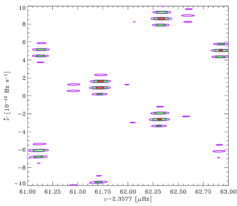
Figure 2: Contour plot of the $Z^{2}_{1}$ power on the $\nu$-$\dot{\nu}$ grid. The purple, green and red contours correspond to $Z^{2}_{1}=250$, 280, and 310, respectively.

4 Origin of the erratic spin behavior

The deviations from monotonic spin-down in 1E1207 are substantial, and they manifest on timescales of years to as short as possibly weeks as evidenced by the phase noise detected here. We now consider four possibilities for both the erratic long-term spin behavior and short-term phase noise in 1E1207: ($i$) frequent glitching, ($ii$) accretion and propeller torques from a circumstellar debris disk, ($iii$) timing noise in an isolated neutron star, and ($iv$) orbital Doppler shifts caused by the presence of a binary companion.

For any glitch model, the glitch frequency and amplitude would have to be very high to account for the observed spin variability (see Zavlin et al. 2004). Moreover, the most viable timing solutions indicating spin down over the 40-day observing span differ from the long-term spin-down of 1E1207 over the last 5.5 years ($\sim-$4 $\times$ $10^{-14}$ Hz s^-1) by an order of magnitude. For example, the most likely spin-down solution (MOD2) has a frequency derivative more than one order of magnitude larger. Because only a very contrived glitch model could account for the long-term frequency history, and this model would provide no explanation for the short-term phase noise, the glitch model is effectively excluded by these observations.

Debris disks left over from the supernova explosions that produce neutron stars could alter the spin evolution of the central neutron star via accretion and propeller torques (Zavlin et al. 2004). If the spin-up rate of 1E1207 during the 40-day interval were equal to the values measured for MOD1 or MOD3, then the mass accretion rate would have to be very large ($\dot{m}>3\times 10^{16}$ g s^-1). Such a large accretion rate would require a large increase in X-ray luminosity which is not observed. Even the spin-down solutions would require significant optical and IR emission from the disk. Deep IR observations of 1E1207 have shown no indication of even a cool, passive debris disk (Wang, Kaplan & Chakrabarty 2006). Thus, it appears unlikely that a debris disk is the cause of the spin variability in 1E1207.

Timing noise (irregular evolution of the pulse phase with time) is a ubiquitous phenomenon in isolated neutron stars. This variability is in addition to the usual variation caused by magnetic braking. It has been demonstrated that the magnitude of these irregular variations depends upon the spin-down rate of the pulsar (e.g., Cordes & Helfand 1980). Millisecond pulsars show the smallest timing noise while magnetars exhibit very strong timing noise. In the case of magnetars, these variations manifest as changes in the effective spin-down rate of up to factors of 5 on a time scale of years. For a convenient (albeit crude) description of timing noise, Arzoumanian et al. (1994) introduced a “stability parameter” defined by the following equation: $\Delta_{\log t}=\log(|\ddot{\nu}|t^{3}/6\nu)$, where $t$ is the time during which the pulse phase has been monitored ($t=10^{8}$ s is a commonly used characteristic time), and $\ddot{\nu}$ is the formal value of the second frequency derivative obtained from fitting a cubic model to pulse phases (it is much larger in magnitude than the actual $\ddot{\nu}$ for noisy pulsars). Third-order polynomial fits to the 1E1207 phase residuals of the top three candidate timing solutions yielded insignificant measurements of $\ddot{\nu}$. The timing observations of 1E1207 during 5.5 years were too sparse to fit the pulse phases with any model. Therefore, to estimate $\ddot{\nu}$ and $\Delta_{8}$, we fitted the dependence $\nu(t)=\nu_{0}+\dot{\nu}(t-t_{0})+\ddot{\nu}(t-t_{0})^{2}/2$ to the frequency history covering the last 5.5 years. (The same exercise was performed by Heyl & Hernquist 1999 for some Anomalous X-ray Pulsars, and it was shown to be reasonably accurate by Gavriil & Kaspi 2004.) Choosing $t_{0}=52700$ MJD TDB, we found $\nu_{0}=2,357,762.8\pm 0.2$ $\mu$Hz, $\dot{\nu}=(-3.4\pm 0.6)\times 10^{-14}$ Hz s^-1, and $\ddot{\nu}=(5.9\pm 1.9)\times 10^{-22}$ Hz s^-2, which translates to a timing noise level of $\Delta_{8}=1.6$. In Figure 3, we show the period derivative versus the timing noise parameter $\Delta_{8}$ for 126 isolated pulsars of various flavors as well as for the CCO 1E1207. The isolated pulsars fall along a relatively well-defined locus, from the quiet millisecond pulsars to the noisy Soft Gamma Repeaters, while 1E1207 stands out from this trend with an anomalously large timing noise strength, some 2$-$4 orders of magnitude higher than isolated pulsars at similar spin-down rates. Although such an estimate for the timing noise parameter is, by necessity, very crude, its enormously high magnitude, together with the gross inconsistency of the local (June-July 2005) spin-down rate with the long-term average, suggest that the erratic frequency behavior in this source is not due to the same effect that causes timing noise in other isolated neutron stars.

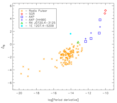
Figure 3: The timing noise parameter $\Delta_{8}$ after Arzoumanian et al. (1994) for 119 radio pulsars, the isolated neutron star RX J0720.4$-$3125 (Kaplan & van Kerkwijk 2005b), four Anomalous X-ray Pulsars (blue squares - Gavriil & Kaspi 2004; blue plus signs - Heyl & Hernquist 1999), two Soft Gamma Repeaters (Woods et al. 2002) and the CCO 1E 1207.4$-$5209.

The most straightforward explanation for the long-term spin variations in 1E1207 is the presence of a binary companion. Note that this model cannot explain the observed short-term phase noise. Current IR and optical limits for 1E1207 exclude main sequence companions earlier than M5 and even white dwarfs with effective temperatures greater than $\sim$10⁴ K (Fesen et al. 2006; Wang et al. 2006). Allowable companion masses are less than 0.2 M_⊙ for late-type stars (Moody et al. 2006, in preparation). Even with such low-mass companions, the resulting Doppler shifts are large enough to account for the frequency variations in 1E1207. Using the archival spin frequencies in combination with the phases from our three candidate timing solutions, we fit the data to a circular orbital model whose phase evolution is defined by the following equation: $\phi(t)=\phi(t_{0})+\nu(t-t_{0})+\frac{1}{2}\dot{\nu}(t-t_{0})^{2}+A\sin{\omega(t-t_{0})}$. This is the same equation as given in §3.1 with an additional sinusoidal term to account for the orbital Doppler shifts. We identified a family of acceptable orbits for each of the three timing solutions listed in Table LABEL:tab:spin. The full set of allowable timing solutions are too numerous to list. We can place only very crude constraints on the orbital periods to fall between 120 and 600 days. The mass functions range between $1\times 10^{-7}$ and $5\times 10^{-5}$ M_⊙ for acceptable orbital solutions. For a 90^∘ inclination and a 1.4 M_⊙ neutron star, the corresponding companion mass range is 0.007 to 0.05 M_⊙, well within the existing limits on companion masses from IR and optical observations. For illustrative purposes, we show two example orbital solutions that are consistent with the existing timing data for 1E1207 (Figure 4).

Figure 4: Candidate orbital solutions for 1E1207 consistent with our MOD2 (top) timing solution and MOD1 (bottom) timing solution.

5 Conclusions

We observed 1E1207 with XMM-Newton seven times during the course of a 40 day interval in an effort to measure the local pulse frequency and frequency derivative with high precision. Due to unanticipated phase noise, we were unable to phase-connect the full data set. From systematic pulse ephemeris searches, we identified a number of possible timing solutions, none of which had spin-down rates close to the average spin-down rate of 1E1207 over the last 5 years. The interpretation of the erratic long-term timing behavior of 1E1207 in terms of the usual pulsar timing noise would require timing noise levels much higher than seen in isolated neutron stars with comparable spin-down rates. The most plausible explanation for the erratic long-term pulse frequency evolution of 1E1207 is the presence of a binary companion, although the current data do not allow us to place strong constraints on system parameters. Further efforts at phase-coherent pulse timing observations of 1E1207 are required to ($i$) unambiguously identify the nature of the long-term pulse frequency variations, and ($ii$) confirm and further investigate the observed short-term phase noise. Just one additional 40-day observing sequence with higher sampling would yield far better constraints on orbital parameters should 1E1207, in fact, possess a binary companion.

- (1) Arzoumanian Z., Nice D.J., Taylor J.H., et al., ApJ, 422, 671 (1994)
- (2) Bignami G.F., Caraveo P.A., De Luca A., et al., Nature, 423, 725 (2003)
- (3) Buccheri R., Bennett K., Bignami G.F., et al., A&A, 128, 245 (1983)
- (4) Cordes, J.M. & Helfand, D.J. ApJ, 239, 640 (1980)
- (5) Fesen R.A., Pavlov, G.G., Sanwal, D., ApJ, 636, 848 (2006)
- (6) Gavriil F.P., Kaspi V.M., ApJL, 609, 67 (2004)
- (7) Hailey C.J., Mori K., ApJL, 578, 133 (2002)
- (8) Heyl J.S., Hernquist L., MNRAS, 340, L37 (1999)
- (9) Kaplan D.L, van Kerkwijk M.H., ApJL, 635, 65 (2005a)
- (10) Kaplan D.L, van Kerkwijk M.H., ApJL, 628, 45 (2005b)
- (11) Mattox, J.R., Halpern, J.P., Caraveo, P.A., A&AS, 120, 77 (1996)
- (12) Mereghetti S., De Luca A., Caraveo P.A., et al., ApJ, 581, 1280 (2002)
- (13) Mori, K., & Hailey, C., astro-ph/0301161, submitted to ApJ (2006)
- (14) Mori K., Chonco J.C., Hailey C.J., ApJ, 631, 1082 (2005)
- (15) Pavlov, G.G., Bezchastnov, V.G.. ApJL, 635, L61 (2005)
- (16) Pavlov, G.G., Sanwal, D., Garmire, G.P.,et al. In: Neutron Stars in Supernova Remnants, ed. P.O. Slane & B.M. Gaensler, ASP Conf. Ser. 271, 247 (2002a)
- (17) Pavlov, G.G., Zavlin V.E., Sanwal D., et al., ApJL, 569, 95 (2002b)
- (18) Pavlov G.G., Sanwal D., Teter M.A., In: IAU Symp. 218, Young Neutron Stars and Their Enviroments, ed. F. Camilo & B.M. Gaensler (San Francisco: ASP), p. 239 (2004)
- (19) Sanwal D., Pavlov G.G., Zavlin V.E., et al., ApJL, 574, 61 (2002)
- (20) Wang Z., Kaplan D.L., Chakrabarty D., ApJ, submitted (astro-ph/0606686)
- (21) Woods P.M., Kaspi, V.M., Thompson, C., et al., ApJ, 605, 378, (2004)
- (22) Woods P.M., Kouveliotou C., Gögüs E., et al., ApJ, 576, 381 (2002)
- (23) Woods P.M., Kouveliotou C., Finger M.H., et al., ApJ, in press (2006; astro-ph/0602531)
- (24) Zavlin V.E., Pavlov G.G., Sanwal D., et al., ApJL, 540, 25 (2000)
- (25) Zavlin V.E., Pavlov G.G., Sanwal D., ApJ, 606, 444 (2004)
- (26) Zavlin V.E., Trümper, J., & Pavlov G.G. ApJL, 525, 959 (1999)