Interstellar abundances in the neutral and ionized gas of NGC604

Abstract

Aims. We present FUSE spectra of the giant H ii region NGC604 in the spiral galaxy M33. Chemical abundances are tentatively derived from far-UV absorption lines and compared to those derived from optical emission lines.

Methods. Absorption lines from neutral hydrogen and heavy elements were observed against the continuum provided by the young massive stars embedded in the H ii region. We derived the column densities of H i, N i, O i, Si ii, P ii, Ar i, and Fe ii, fitting the line profiles with either a single component or several components. We used CLOUDY to correct for contamination from the ionized gas. Archival HST/STIS spectra across NGC604 allowed us to investigate how inhomogeneities affect the final H i column density.

Results. Kinematics show that the neutral gas is physically related to the H ii region. The STIS spectra reveal H i column density fluctuations up to 1 dex across NCG604. Nevertheless, we find that the H i column density determined from the global STIS spectrum does not differ significantly from the average over the individual sightlines. Our net results using the column densities derived with FUSE, assuming a single component, show that N, O, Si, and Ar are apparently underabundant in the neutral phase by a factor of $\sim 10$ or more with respect to the ionized phase, while Fe is the same. However, we discuss the possibility that the absorption lines are made of individual unresolved components, and find that only P ii, Ar i, and Fe ii lines should not be affected by the presence of hidden saturated components, while N i, O i, and Si ii might be much more affected.

Conclusions. If N, O, and Si are actually underabundant in the neutral gas of NGC604 with respect to the ionized gas, this would confirm earlier results obtained for the blue compact dwarfs, and their interpretations. However, a deeper analysis focused on P, Ar, and Fe mitigates the above conclusion and indicates that the neutral gas and ionized gas could have similar abundances.

1 Introduction

The interstellar medium (ISM) is mainly enriched by heavy elements produced by the young massive stars during many starburst episodes taking place over the star-formation history of the galaxy. The immediate fate of metals released by these massive stars in the H ii regions where stars recently formed, has not yet been settled. Kunth & Sargent (1986) have suggested that the H ii regions of the blue compact dwarf galaxy IZw 18 enrich themselves with metals expelled by supernovæ and stellar winds during the timescale of a starburst episode (i.e., a few $10^{6}$ yr). However, observational evidence (see e.g., Martin et al. 2002) shows that metals might be contained in a hot phase reaching the halo of galaxies, before they could cool down and eventually mix into the ISM. The issue of the possible self-enrichment of H ii regions is essential to understanding the chemical evolution of galaxies, since H ii region abundances derived from the optical emission lines of the ionized gas are extensively used to estimate the metallicity of galaxies. If there is self-pollution of these regions, the derived abundances would no longer reflect the actual abundances of the ISM.

One approach to studying possible self-enrichment and, more generally, the mixing of heavy elements in the ISM is to compare the abundances of the ionized gas to those of the surrounding neutral gas. A first attempt was made by Kunth et al. (1994) using the GHRS onboard the Hubble Space Telescope (HST). These authors derived the neutral oxygen abundance in IZw 18 using the O i $\lambda$1302 line arising in absorption and using the H i column density and velocity dispersion from radio observations. They found an oxygen abundance that is 30 times lower than in the ionized gas. However, the result remains inconclusive since the O i line is likely to be heavily saturated, so that its profile could be reproduced with a solar metallicity by choosing a different dispersion velocity parameter, as pointed out by Pettini & Lipman (1994).

The Far Ultraviolet Spectroscopic Explorer (FUSE; Moos et al. 2000) gives access to many transitions of species arising in the neutral gas, including H i, N i, O i, Si ii, P ii, Ar i, and Fe ii, with a wide range of oscillator strengths for most of the species. Hence it becomes possible to determine abundances in the neutral gas with better accuracy.

A surprise came from recent FUSE studies of five gas-rich blue compact metal-poor galaxies (BCDs): IZw 18 (Aloisi et al. 2003; Lecavelier et al. 2004), Markarian 59 (Thuan et al. 2002), IZw 36 (Lebouteiller et al. 2004), SBS 0335-052 (Thuan et al. 2005), and NGC625 (Cannon et al. 2004). In these galaxies, nitrogen seems to be systematically underabundant in the neutral gas with respect to the ionized gas of the H ii regions. The oxygen abundance seems either lower in the neutral gas or similar to the one in the ionized gas. This picture, if true, could offer a new view of the chemical evolution of the ISM in a galaxy, especially for the metal dispersion and mixing timescales. It could, however, suffer from uncertainties such as ionization corrections, depletion effects, or systematic errors due to the multiple sightlines toward individual stars and, possibly, multiple H ii regions within the spectrograph entrance aperture.

In this respect, nearby giant H ii regions in spiral galaxies provide an interesting case, since only one H ii region fits the aperture. Moreover, their resolved young stellar population can be investigated to analyze the stellar continuum and in order to understand and correct for the effects of having multiple sightlines contributing to the absorption line profiles. NGC604 is the first nearby giant H ii region we have investigated for this purpose. It is a young star-forming region in the dwarf spiral galaxy M33 with an age of 3-5 Myr (e.g., D’Odorico & Rosa 1981; Wilson & Matthews 1995; Pellerin 2006). NGC604 is the brightest extragalactic H ii region in the sky after 30 Doradus. It is located about 12’ from the center of M33. At a distance of 840 kpc (Freedman et al. 1991), 1” corresponds to 4.1 pc. The nebula has a core-halo structure, where the core has an optical diameter of $\sim 220$ pc and the halo a diameter of $\sim 440$ pc (Melnick 1980). The optical extinction in NGC604 appears to be correlated with the brightness. It is highest toward the brightest regions ($A_{V}=1.7\textrm{-}2.8$ mag), while the average extinction over the nebula is $A_{V}\sim 0.5$ mag, suggesting that dust is correlated with the ionized gas (Churchwell & Goss 1999, Viallefond et al. 1992).

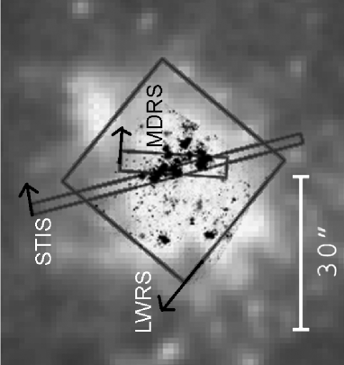
Figure 1: FUSE and HST/STIS apertures are plotted over the optical image from the POSS2 survey (B band). We superimposed the most massive stars in black as observed with STIS at 2000 Å. The arrows show the dispersion direction for each slit. North is up.

We first describe the observations in Sect. 2 and the data analysis in Sect. 3, with particular emphasis on the influence of the source extent on the absorption line profiles. In Sect. 4 we analyze the diffuse molecular hydrogen content, while in Sect. 5 we infer the neutral hydrogen column density. Metal column densities in the neutral gas are discussed in Sect. 6. We estimate the neutral gas chemical composition in Sects. 7 and 8 and eventually compare it with the ionized gas of the H ii region. Finally, in Sect. 9, we investigate how the presence of hidden saturated unresolved absorption components can be a major problem for determining the column density.

2 Observations

The ionizing cluster of NGC604 was observed with the FUSE telescope through the MDRS and LWRS entrances (see the log of the observations in Table 1). The source as observed in the far-UV, with an apparent size of $\sim$10”$\times$15” (see Fig. 1), should be considered as extended relative to the size of the apertures. Data were recorded through the LiF and SiC channels ($\sim 1000\textrm{-}1200$ Å and $\sim 900\textrm{-}1100$ Å resp.). These channels are independently calibrated and provide redundant data, making it possible to identify possible instrumental artifacts. The data were processed with the CalFuse $2.4$ pipeline. Figure 2 shows the LWRS spectrum over the full spectral range $\sim 900\textrm{-}1200$ Å. Apart from the lines of neutral species, a remarkable detection is the interstellar O vi line in NGC604, tracing hot gas, at a radial velocity of $-211\pm 25$ km s^-1($\lambda=1031$ Å). We did not observe any significant differences in the extracted spectrum whether correcting for the jitter of the satellite or not.

Table 1: Log of the observations.

	FUSE	FUSE	HST/STIS	IUE
PID	B018	A086	9096
Date	12/2003	09/2001	08/1998	1979-1984
Range (Å)	900-1200	900-1200	1150-1730	1150-1950
Exp. (ksec)	7	13	2	4.8-22.8
Aperture	4”$\times$20”	30”$\times$30”	52”$\times$2”	$\approx$10”$\times$20”
	(MDRS)	(LWRS)	G140L	SWP
Resolutiona	0.07 Å	0.07 Å	2 Å	5 Å

• Spectral resolution for a point-like source.

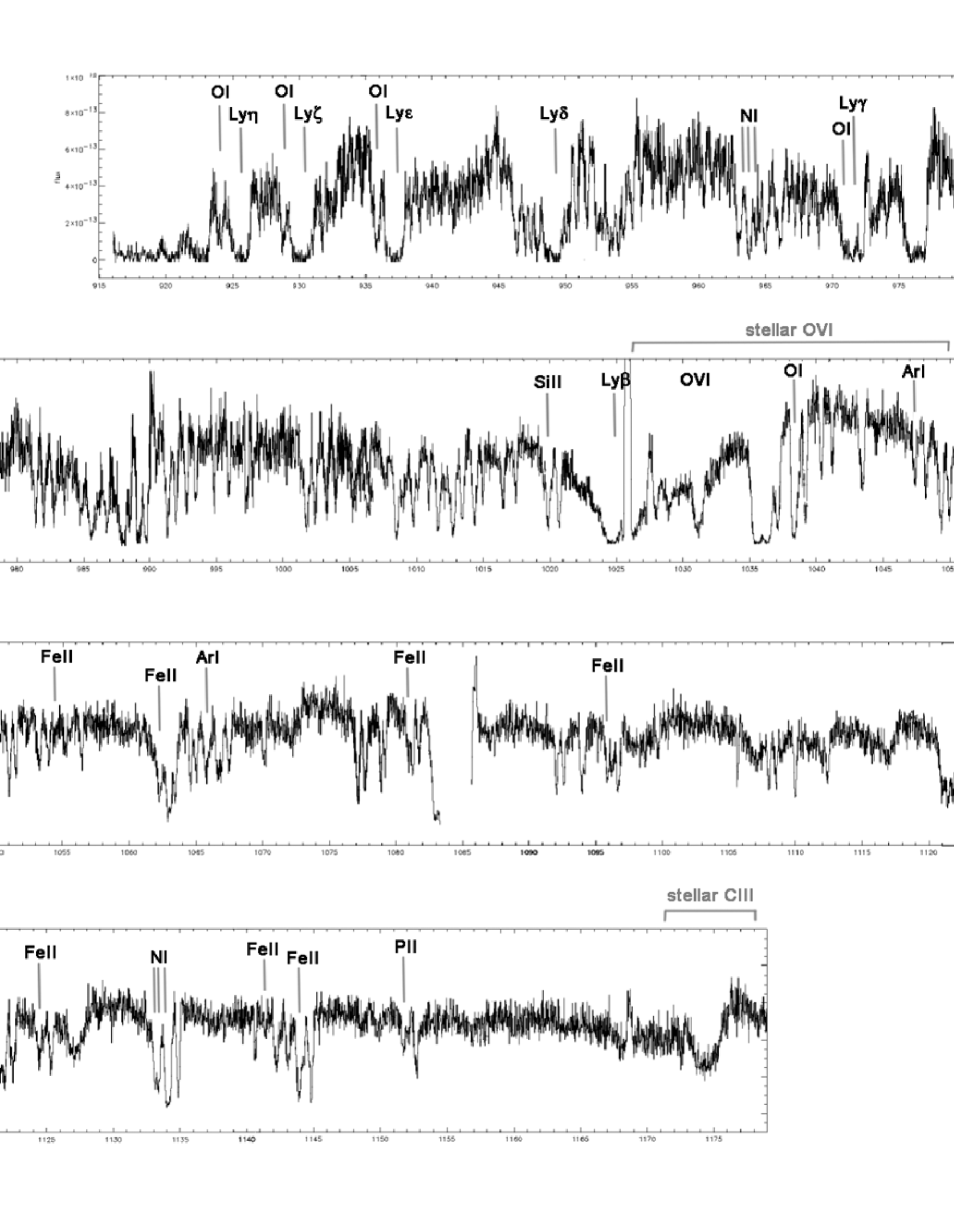
Figure 2: FUSE LWRS spectrum of NGC604, indicating the most prominent interstellar lines from NGC604. We also show the wavelength ranges of the two broad O vi and C iii stellar P Cygni profiles.

We investigated the neutral gas inhomogeneity by using HST/STIS spectra toward individual stars in the ionizing cluster (Sect. 5.4). These spectra were taken with the G140L grating using the FUV-MAMA detector, and have been kindly provided to us by F. Bruhweiler and C. Miskey. The extraction technique is described by Miskey et al. (2003).

We also used IUE archival data in the short-wavelength low-resolution mode to determine the H i content in NGC604 using the Ly$\alpha$ line (Sect. 5.3). We analyzed 10 IUE spectra with exposure times longer than $\sim 5$ ksec.

3 Data analysis

The most plausible physical situation in NGC604 is the presence of clouds with different physical properties that produce different absorption line components. Indeed, the multiple sightlines toward the massive stars in the NGC604 cluster contribute to the global spectrum of the region. However, due to resolution effects, we only observe a single component, and this is the assumption we make in a first analysis presented in this section. Jenkins et al. (1986) found that this assumption, even in the case of complex sightlines, does not yield significant systematic errors on the column density determination, unless very strongly saturated lines are present. We discuss this issue in detail in Sect. 9.

3.1 The profile fitting method

The interstellar absorption lines we observe appear symmetric and can be reproduced by a Voigt profile. We detect lines arising from both NGC604 and the Milky Way clouds lying along the sightline. The NGC604 absorption component is blue-shifted by $\sim-250$ km s^-1 ($\sim 0.8$ Å) with respect to the Galactic component ($\sim 0$ km s^-1). Another weaker absorption component is found at $\sim-150$ km s^-1, which is likely to be associated with a high velocity cloud in M33.

The data analysis was performed using the profile fitting procedure Owens (Lemoine et al. 2002) developed at the Institut d’Astrophysique de Paris by Martin Lemoine and the FUSE French Team. This program returns the most likely values of many free parameters such as temperatures ($T$), radial velocities ($v$), turbulent velocity dispersion ($b$), and column densities ($N$) of species, by a $\chi^{2}$ minimization of the fits of the absorption line profiles. The program also allows changes in the shape and intensity of the continuum, in the line broadening, and in the zero level. The errors on the $N$, $b$, $v$, and $T$ parameters are calculated using the $\Delta\chi^{2}$ method described in Hébrard et al. (2002), and they include the uncertainties on all the free parameters (notably the continuum level and shape). All the errors we report are within $2\,\sigma$.

The Owens procedure is particularly suited to far-UV spectra overcrowded with absorption lines, since it allows for a simultaneous fit of all lines in a single spectrum. This method allows us to investigate blended lines with minimum systematic errors: for example, an Fe ii line that is blended with an H₂ line can still be used to constrain the Fe ii column density, since the H₂ column density is well-constrained by all the other H₂ lines fitted simultaneously in the spectrum.

We derived column densities from profile fitting using two different approaches:

• Simultaneous fit. Species are arranged in several groups, each group defined by common $b$, $T$, and $v$ parameters. One group refers to species that we assume to be mainly present in the neutral phase (i.e., H i, N i, O i, Si ii, P ii, Ar i, and Fe ii), another group corresponds to the molecular hydrogen H₂, another one to the interstellar O vi, and the last group refers to the other minor species, mainly higher ionization states.

• Independent fits. Species may not entirely coexist in the same gaseous phase, hence we no longer assume similar $b$, $T$, and $v$. Each species is defined by its own physical parameters.

We are able to use the NGC604 spectra to compare the two approaches and to discuss in particular the reliability of the simultaneous-fit method. This one was indeed preferred for spectra of blue compact dwarf galaxies (see the references in the introduction) $-$ generally because of a relatively low signal-to-noise ratio $-$ but could introduce systematic errors with respect to the more realistic independent-fit method.

3.2 Stellar contamination and continuum

In our observations, the continuum arises from the combination of the spectra of numerous UV bright stars.

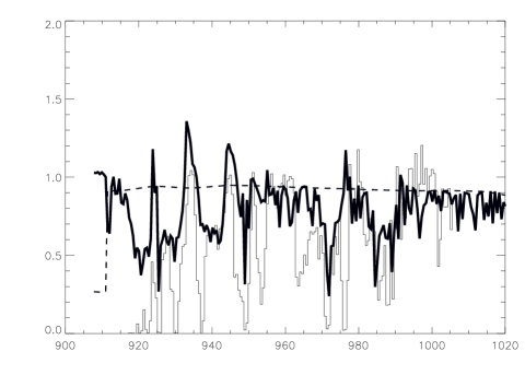
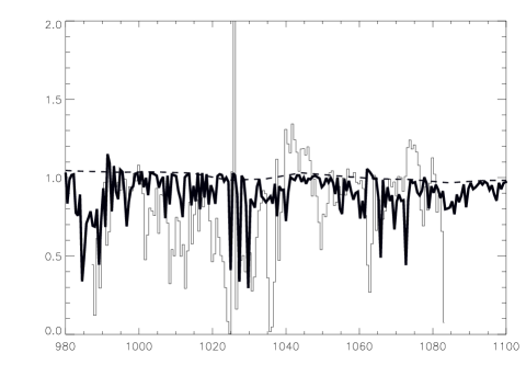
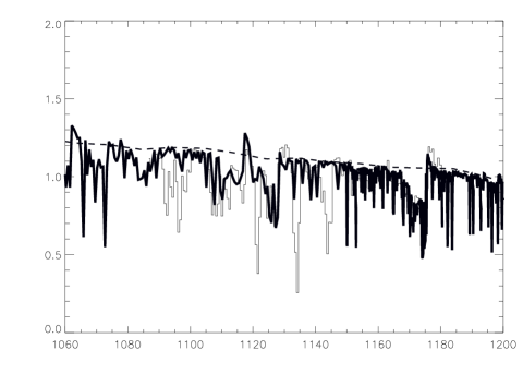
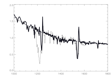
Figure 3: Theoretical stellar spectra (thick solid lines) are overplotted onto the observed FUSE and HST/STIS data (histograms). The flux (in arbitrary units) is plotted versus the wavelength (Å) for the three spectral regions between 900 Å and 1200 Å (FUSE wavelength range), and for the spectral window 1200-1800 Å (STIS wavelength range).

Contamination by stellar absorption lines could be an issue for the interstellar line fitting, especially for H i. However, the contribution of the photospheric H i lines becomes significant only when early B stars dominate (Gonzalez et al. 1997), i.e., for bursts older than $\sim 10$ Myr (Robert et al. 2003). The age of the burst in NGC604 is $\sim$3-5 Myr (see introduction). Hence, given this relatively young age, we expect the photospheric H i lines to be relatively narrow, and their contribution to be negligible as compared to the interstellar damped profile. We verified this assumption by comparing the observed FUSE and HST/STIS spectra with an ad hoc Starburst 99 synthetic model of a young stellar population. The latter was kindly provided by C. Leitherer and F. Bresolin (private communication), and it makes use of a new library of theoretical stellar atmospheres that does not include interstellar absorption lines. The adopted spectra assume an instantaneous 3.5 Myr old burst and a gas metallicity of 0.4 Z_⊙. The interstellar H i lines (see for instance Ly$\beta$ at 1025.7 Å and Ly$\alpha$ at 1215.7 Å) are not significantly contaminated by the $-$ relatively narrow $-$ photospheric lines (see Fig. 3). Notice that the region around the O vi ($\sim 1040$ Å) stellar line is not reproduced well because the input physics is still missing from the theoretical stellar atmosphere models we use.

This synthetic spectral model was also used as a safety check to compare with $-$ but not to constrain $-$ the continuum we adopted for the line profile fitting with Owens (see next sections), and no significant differences were found.

3.3 Influence of the apparent extent of the UV cluster on the line profiles

Interstellar absorption lines are broader in the FUSE LWRS spectrum than in the MDRS spectrum. The line broadening results from the convolution of several effects:

• The intrinsic line width, due to the thermal and the turbulent velocities. Considering the large turbulent velocities usually measured in BCDs and in NGC604 (see Sect. 6.1), the thermal component should be negligible:
  $\Delta\nu_{D}=\frac{\nu_{0}}{c}\times\sqrt{\frac{2kT}{m}+b^{2}}\approx\frac{\nu_{0}}{c}\times b$,
  where $\nu_{0}$ is the frequency and $m$ the mass of the species under consideration.

• The radial velocity dispersion of the clouds within the aperture. This effect is expected to be weaker for a single H ii region than for observations of entire galaxies containing several H ii regions.

• The instrumental line spread function (LSF). For bright point-like sources observed with FUSE, the FWHM of the LSF is $\sim 12$ pixels, i.e., $\sim 20$ km s^-1 (Hébrard et al. 2002).

• The misalignments of the individual sub-exposures. The final spectrum results from the co-addition of several exposures with possible wavelength shifts between individual spectra. This unavoidably introduces some misalignments because of the relatively low signa-to-noise ratio of each exposure. However, given the relatively good quality of the NGC604 observations, the misalignments do not yield a significant additional broadening.

• Finally, the spatial distribution of the UV-bright stars along the slit dispersion axis that results in wavelength smearing.

When comparing the FUSE spectra with the two different apertures, only the geometric effect due to the distribution of the massive stars within the apertures is likely to vary significantly. The Owens procedure makes it possible to estimate the line broadening parameter, which accounts for all the effects mentioned above, except the intrinsic line width, implying the turbulent velocity and the temperature, which is treated independently. Hence, we have here the opportunity of quantifying in a first approximation the aperture effects related to the observation of an extended source.

The most likely value of the line-broadening parameter for the MDRS (4”$\times$20” aperture) spectrum is $\sim 15$ pixels (i.e., $\sim 25$ km s^-1), which is close to the point-source LSF. By taking into account that a 30” source spreads the line by 100 km s^-1 (60 pixels), this translates into a spatial extent of about 5”, which is comparable to the size of the MDRS aperture in the dispersion direction. The most likely broadening value for the LWRS (30”$\times$30”) data is instead about 30 pixels. This is equivalent to a spatial extent of 16”, which is smaller than the size of the aperture and therefore would correspond to the actual extent of the UV bright stellar cluster (see the HST/STIS image at 2000 Å for comparison in Fig. 1).

As a conclusion, the line broadening parameter we infer for the FUSE observations is consistent with the extent of the source at the observed wavelength as constrained by the aperture size. The column densities derived in Sect. 6.2 take this broadening effect into account.

4 Molecular hydrogen

Table 2: H₂ column densities derived from the two FUSE observations. Errors are at $2\sigma$.

	H2,J=0	H2,J=1	H2,J=2	H2,J=3	H2,J=4	H${}_{\rm{2,tot}}^{\mathrm{a}}$
LWRS	$16.39^{+0.20}_{-0.29}$	$16.51^{+0.23}_{-0.31}$	$15.12^{+0.49}_{-0.53}$	$16.17^{+0.30}_{-0.57}$	$14.40^{+0.48}_{-0.60}$	$\textbf{16.86}^{+0.25}_{-0.34}$
detection levelb	$\sim 12\sigma$	$\sim 14\sigma$	$\sim 7\sigma$	$\sim 13\sigma$	$\sim 4\sigma$
MDRS	$16.08^{+0.32}_{-0.47}$	$16.60^{+0.16}_{-0.28}$	$15.08^{+0.58}_{-1.20}$	$16.29^{+0.22}_{-0.39}$	$14.30^{+1.12}_{-3.30}$	$\textbf{16.86}^{+0.23}_{-0.36}$
detection levelb	$\sim 6\sigma$	$\sim 6\sigma$	$\sim 2.5\sigma$	$\sim 6\sigma$	$\sim 2\sigma$

• Value obtained by summing over all detected rotational states.

• Calculated with the $\Delta\chi^{2}$ method, using all the observed lines.

FUSE gives access to many molecular hydrogen lines of the Lyman and Werner bands. The H₂ lines arising from Galactic clouds along the sightline are clearly present in our spectra at the radial velocity of $4\pm 5$ km s^-1. These lines are responsible for blending other atomic lines, including lines of the neutral species in NGC604. However, the column density of each rotational state of the Galactic H₂ is well-constrained given the large number of lines available, allowing correction for this blending effect.

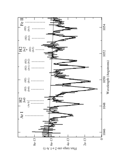
Figure 4: Detection of molecular hydrogen lines (at $\sim 1048.4$ Å and $\sim 1052.3$ Å) arising in NGC604. The thick line represents the fit to the data (histogram, FUSE MDRS spectrum). Lines labelled between parentheses refer to the Milky Way component, the others arise in NGC604.

In contrast to Bluhm et al. (2003), we detected H₂ in NGC604 in both LWRS and MDRS spectra (see Fig. 4). This positive detection has been enhanced by the opportunity given by the Owens procedure to fit simultaneously $-$ and thus gathering all the information of $-$ all the H₂ absorption lines.

The velocity we infer for H₂ lines in NGC604 is $-250.4\pm 2.1$ km s^-1 in the LWRS observation and $-252.2\pm 3.4$ km s^-1 in the MDRS. We did not detect H₂ from the weak absorption component at $\sim-150$ km s^-1. In Table 2 we report the detection levels and the column densities of each rotational state. We used these column densities to build the excitation diagram of Fig. 5. The ratio between the H₂ column densities in the $J=1$ and $J=0$ levels (ortho- to para-hydrogen) yields a rotational temperature of $T=112\pm 10$ K. This temperature can be identified as the gas kinetic temperature, since these two rotational states should be populated mainly by collisional processes. The higher excitation of levels $J=3$ and $J=4$ is common in the ISM and is due to non-collisional processes, such as UV photon pumping, shocks, and formation of H₂ on dust grains.

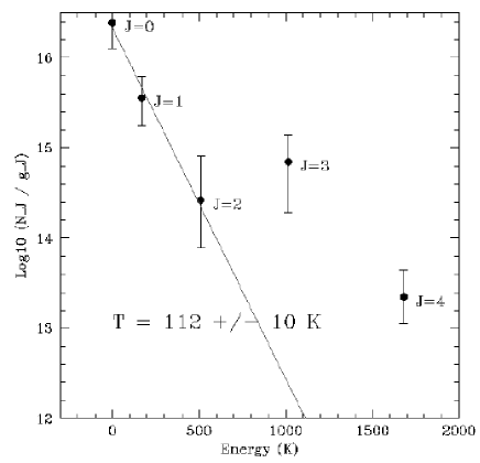
Figure 5: Excitation diagram of the diffuse H₂ in NGC604. Column densities of the H₂ rotational levels divided by their statistical weights are plotted against their excitation energies. The ratio of $J=1$ to $J=0$ levels yields a rotational temperature $T=112\pm 10$ K.

Given the fact that upper rotational states ($J>4$) are not detected, we choose to neglect their contribution to calculate the total molecular hydrogen column density which is found to be $\log N(\rm{H}_{2})=16.86^{+0.25}_{-0.34}$. The molecular fraction defined as $f_{\rm{H2}}=2\times N(\textrm{H}_{2})/[2\times N(\textrm{H}_{2})+N(\textrm{H\,{\sc i}})]$ is then $2.6\times 10^{-4}$ (see Sect. 5 for the adopted value of the H i column density). Such a low value can seem somewhat surprising in a star-forming region considering that H₂ is an important gas reservoir in which to form stars. Hoopes et al. (2004) found similarly low fractions in their sample of starburst galaxies, where upper limits of $f_{\rm{H2}}$ range from $4.9\times 10^{-6}$ to $1.6\times 10^{-4}$. It is likely that the diffuse molecular hydrogen is destroyed by the incident UV flux from the massive stars in the star-forming region. Most of the remaining molecules should be in dense clumps, which are opaque to far-UV radiation, and do not contribute to the observed spectra (Vidal-Madjar et al. 2000; Hoopes et al. 2004).

5 Neutral hydrogen toward NGC604

The broad interstellar H i absorption measured toward NGC604 cluster results from the blended lines arising in the Milky Way, in NGC604, and in the weak component at $\sim-150$ km s^-1. Note that, given the intermediate velocity of the latter, its H i absorption falls in the heavily saturated core of the main H i absorption line. Therefore, this component does not significantly modify the integrated H i absorption line profile along the sightline.

5.1 Galactic component

Interstellar clouds of the Milky Way contribute to the absorption line spectra toward NGC604. However, according to Velden (1970), the Galactic H i column density is expected to be somewhat lower than the intrinsic H i component. From the survey of Heiles (1975), the Galactic H i column density should be a few $10^{20}$ cm^-2. This is consistent with the estimates we obtained from the reddening of E(B-V)=0.09 (Israel & Kennicutt 1980). Indeed, by assuming that $N_{\rm{HI}}/\textrm{E(B-V)}=5.8\times 10^{21}$ cm^-2 mag^-1 (Bohlin et al. 1978), we find a Galactic H i column density of $\log N\textrm{(H\,{\sc i})}\approx 20.7$ (where the column density is expressed in atom cm^-2). This value agrees well with our estimate obtained from the FUSE data (see Sect. 5.2).

5.2 FUSE observations of Ly$\beta$

The H i Lyman lines from Ly$\beta$ to Ly$\mu$ fall within the FUSE wavelength range. However, in order to infer the H i column density from FUSE spectra, we can only reliably use Ly$\beta$, since it is the only H i line showing damping wings. The other Lyman lines fall in the flat part of the curve of growth, where there is degeneracy between the turbulent velocity and the column density. In addition, the higher-order H i Lyman lines are located in spectral regions that are more crowded by other contaminating absorption lines (e.g., Galactic H₂ or other atomic interstellar lines).

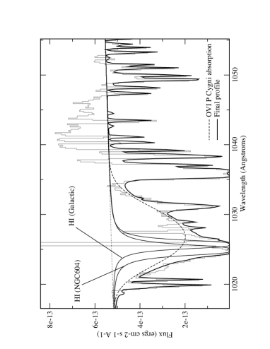
Figure 6: The interstellar Ly$\beta$ profile as observed in the FUSE LWRS spectrum is heavily contaminated by the stellar O vi P Cygni doublet absorption. The emission component of the latter was not accounted for in the fitting (see text). For display purposes, all the other interstellar absorption lines are not marked, and data are rebinned by a factor 8.

Nevertheless, the H i Lyman $\beta$ line in NGC604 is contaminated by the stellar O vi P Cygni doublet at 1031.9 Å and 1037.6 Å, as also observed by Cannon et al. (2004) in the starburst galaxy NGC625. The two stellar lines are heavily blended, resulting in a broad P Cygni shaped line. In an attempt to model the stellar O vi feature in order to further estimate the interstellar H i absorption, we decided to reproduce the absorption component of the total P Cygni profile using a Gaussian profile. This is a rough approximation since the theoretical asymmetrical P Cygni profile should be used instead. However, one can reasonably expect the global profile, which is the combination of the individual profiles of different types of stars, to have a roughly symmetrical absorption component (the C iii, C iv, and Si iv stellar absorptions indeed appear symmetrical in the FUSE and IUE spectra). We performed a simultaneous fit of the interstellar lines, in particular the H i line Ly$\beta$ in NGC604, together with the broad O vi stellar absorption. The velocity shift and the width of the latter were allowed to vary without any constraints. The emission component of the P Cygni profile was ignored for the fitting.

The best result, corresponding to the minimum $\chi^{2}$, is shown in Fig. 6. The stellar absorption has a likely width of $\sim 1300$ km s^-1 and a blue shift of $\sim-1500$ km s^-1. An H i column density of $\log N\textrm{(H\,{\sc i})}=20.7$ was derived for the Milky Way component (estimated uncertainty 0.3 dex at 2 $\sigma$), while a value of $\log N\textrm{(H\,{\sc i})}=20.75$ ($\pm 0.3$, see Fig. 7) was inferred for the H i in NGC604.

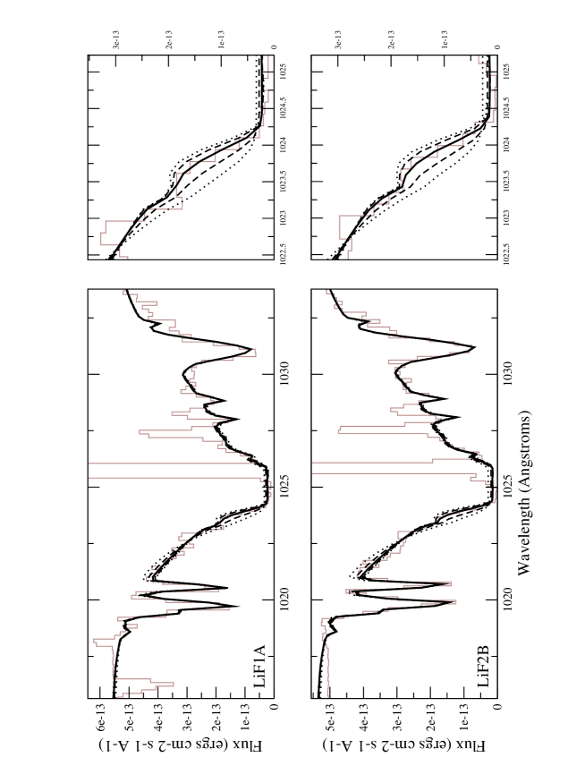
Figure 7: Profiles for an H i column density in NGC604 of $\log N\textrm{(H\,{\sc i})}=20.75$ (thick line), $\log N\textrm{(H\,{\sc i})}=20.75\pm 0.30$ (dashed lines), and $\log N\textrm{(H\,{\sc i})}=20.75\pm 0.60$ (dotted lines). Column densities of other species (including Galactic H i) are considered as free parameters in the fitting routine.

5.3 IUE observations of Ly$\alpha$

The H i column density can also be determined from the Ly$\alpha$ absorption signature in low-resolution SWP-IUE spectra (see Table 1). We investigated Ly$\alpha$ from 10 independent spectra (Table 3).

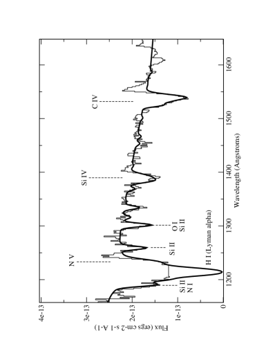
Figure 8: Example of a IUE spectrum toward NGC604. The thick line represents the fit to the data (histogram). Lines marked upwards are stellar in origin. The other lines are interstellar. The airglow emission around 1210 Å has been removed. The emission components of the P Cygni profiles have not been taken into account in the profile fitting.

For the profile fitting, we used the Galactic H i value of $\log N\textrm{(H\,{\sc i})}=20.7$, which is our best guess from the FUSE observations. In each spectrum, Ly$\alpha$ is blended with a single stellar N v P Cygni profile (see Fig. 8). To estimate this contamination, we decided to model the stellar N v absorption component using the same technique as in the previous section. The mean width of the stellar absorption N v in the IUE spectra was found to be $\sim 1200\pm 200$ km s^-1 and the mean velocity shift $\sim-1600\pm 150$ km s^-1. As a result, we inferred a mean H i column density in NGC604 of $\log N\textrm{(H\,{\sc i})}=21.07^{+0.17}_{-0.24}$.

Table 3: H i column density determinations (in cm^-2, logarithmic units) derived from the IUE spectra of NGC604.

Dataset	Exp. Time (ksec)	$\log N$(H i)
swp16034	10.8	$20.99^{+0.27}_{-0.72}$
swp16035	11.3	$21.17^{+0.12}_{-0.19}$
swp19154	18.0	$<21.30^{\textrm{a}}$
swp19181	15.3	$21.02^{+0.16}_{-0.20}$
swp24509	15.6	$20.85^{+0.11}_{-0.14}$
swp04162	4.8	$21.21^{+0.22}_{-0.40}$
swp05682	6.0	$21.01^{+0.29}_{-0.68}$
swp06638	4.8	$<21.33^{\mathrm{a}}$
swp07349	6.4	$21.27^{+0.07}_{-0.05}$
swp24508	5.4	$20.87^{+0.13}_{-0.09}$
Mean column density		$21.07^{+0.17}_{-0.24}$

• The H i Ly$\alpha$ absorption is severely contaminated by a terrestrial airglow.

5.4 H i inhomogeneities revealed by STIS

The H i column density derived from FUSE and IUE spectra could be different from the true H i column density, due to the presence of multiple unresolved absorbers along the many contributing sightlines. We investigated this issue and inquired how the result is affected by the inhomogeneities in the H i by analyzing individual stellar spectra from the long-slit, spatially resolved, HST/STIS data. A few sightlines were impossible to investigate because of edge effects in the MAMA detector, together with a location of the star at the border of the slit.

We first performed a profile fitting of Ly$\alpha$ in the single stellar spectra in order to infer the column density of the H i for each sightline. We adjusted the profile of the stellar N v line using the method described in the previous sections. We also assumed that the Galactic H i column density is identical for all the sightlines, given the relatively low angular extent of NGC604. The results of the profile fitting are reported in Table 4. We find variations up to 1 dex in the H i column density of NGC604, as compared to the uncertainties on the order of $\lesssim 0.4$ dex, suggesting inhomogeneities of the diffuse neutral gas in front of the ionizing cluster. This could be a source of systematic errors when determining the total column density from the integrated light of the cluster. However in our case, the mean value of the H i column density over each single sightline is comparable to the mean value weighted by the star luminosity (see Table 4), which is what we actually measure in the global spectrum of a star cluster.

Table 4: H i column density toward individual stars of NGC604 cluster, as derived from the Ly$\alpha$ line detected with HST/STIS.

Stara	Spectral typea	Flux at $\sim$1280 Åb	$\log N$(H i)
117	O4 II	4.0	$20.26^{+0.29}_{-0.40}$
564	O9 II	2.8	$20.95^{+0.16}_{-0.19}$
578b	O9 Ia	4.5	$20.87^{+0.05}_{-0.16}$
675	O7 II	2.8	$21.33^{+0.16}_{-0.13}$
690a	O5 III	1.8	$20.78^{+0.36}_{-0.75}$
690b	B0 Ib	3.4	$20.62^{+0.26}_{-0.40}$
825	O5 II	3.5	$20.36^{+0.36}_{-1.32}$
867a	O4 Iab	10.0	$20.70^{+0.25}_{-0.44}$
867b	O4 Ia	22.0	$20.71^{+0.29}_{-0.49}$
Mean column density			$20.84^{+0.20}_{-0.26}$
Flux-weighted mean column density			$20.77^{+0.23}_{-0.33}$

• From Miskey et al. (2003).

• In units of $\times 10^{-15}$ ergs cm^-2 s^-1 Å^-1.

In addition, we synthesized the global spectrum within the STIS 52”$\times$2” slit, summing each one of the extracted stellar spectra. In this way, we simulated the spectral observation of a cluster as a whole, i.e., our FUSE observations. Given the relatively high dispersion of the G140L grating ($\sim 2$ Å), combined with the width of the STIS slit, different positions of stars within the slit can lead to in a relative wavelength shift up to several thousands of km s^-1. We thus corrected the data for these shifts. This allowed us to reach an accuracy on the order of 1 pixel, corresponding to a velocity dispersion of less than $\sim 150$ km s^-1, comparable to the wavelength smearing along the FUSE LWRS aperture ($\sim 50$ km s^-1, Sect. 3.3). From the Ly$\alpha$ profile of this summed spectrum (see Fig. 9), we obtained a column density of $\log N\textrm{(H\,{\sc i})}=20.67^{+0.19}_{-0.22}$ for the H i in NGC604. This estimate is consistent within the errors with the ”simple” and ”luminosity-weighted” means reported in Table 4. This indicates that, in our integrated spectra, we are not misestimating the actual column density, even though the absorption arises from many sightlines intersecting clouds with different physical properties.

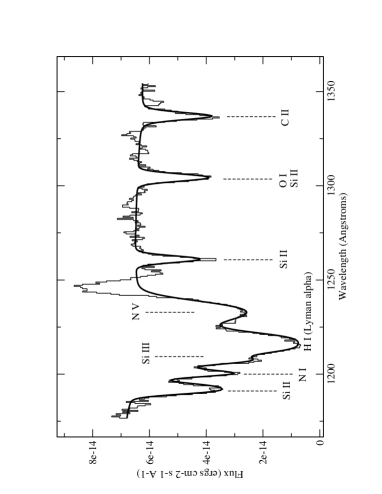
Figure 9: Profile fitting of the Ly$\alpha$ line from the global HST/STIS spectrum (obtained by summing the individual extracted stellar spectra). See Fig. 8 for a description of the plot.

5.5 The adopted H i column density in NGC604

Table 5: H i column density determinations using FUSE, IUE and HST/STIS data.

Instrument	Line	Remarks	Value
FUSE	Ly$\beta$	Corrected for the stellar O vi contamination	$20.75\pm 0.30$
IUE	Ly$\alpha$	Mean value of the sample spectra	$21.07^{+0.17}_{-0.24}$
HST/STIS	Ly$\alpha$	Mean value from the individual star spectra	$20.84^{+0.20}_{-0.26}$
HST/STIS	Ly$\alpha$	Flux-weighted mean value from the individual star spectra	$20.77^{+0.23}_{-0.33}$
HST/STIS	Ly$\alpha$	Profile fitting of the global spectrum	$20.67^{+0.19}_{-0.22}$
Radio	21 cm line	Quantity of H i in the whole region	$\sim 21.4$
Adopted column density for metal abundance derivations			$20.75\pm 0.30$

In Table 5 we report the various determinations obtained for the H i column density in NGC604. The neutral hydrogen was also investigated using radio observations. Israel et al. (1974) noticed a correlation between H ii region locations and large H i complexes in M33. By measuring the H i column density with the 21 cm line in emission, Dickey et al. (1993) found $\log N\textrm{(H\,{\sc i})}=21.38\pm 0.01$ ($45\textrm{"}\times 45\textrm{"}$ beam), while Newton (1980) found $21.43\pm 0.50$ ($47\textrm{"}\times 93\textrm{"}$ beam). The direct comparison between these measurements, which sample the H i in all the region, and the H i detected in absorption in front of the stellar cluster is not straightforward. Hence we only notice that the H i quantity measured in emission is larger than the one measured in absorption, which is what is expected given the source geometry. From now on we adopt the FUSE value for our abundance studies in the neutral medium, i.e., $\log N\textrm{(H\,{\sc i})}=20.75\pm 0.30$. This value, together with these errors, agrees closely with all the other determinations.

6 Heavy elements

We were able to identify many absorption lines in the FUSE spectra arising from heavy elements in the neutral ISM of NGC604 (see Fig. 2). From the profile fitting of these lines, we derived the turbulent velocities, radial velocities, and column densities of each species. The complete list of the lines we analyzed is reported in Table 6. In Fig. 10, we show the example of the $\lambda 1125.4$ Fe ii line profile fitting.

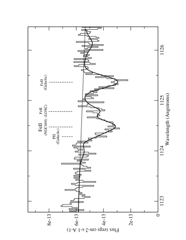
Figure 10: Result of the profile fitting method for the Fe ii line at 1125.4478 Å. Three absorption components are detected, NGC604, the line of sight cloud (LOSC) at $\sim-150$ km s^-1, and the Galactic component.

Table 6: Analyzed lines of the metallic species in NGC604, where $f$ is the oscillator strength, $\lambda_{\rm{rest}}$ the rest wavelength (from the tables of Morton 1991 & 2003), and $\lambda_{\rm{obs}}$ the observed wavelength as obtained with the independent fit method applied to the LWRS FUSE spectrum.

Species	$\lambda_{\rm{rest}}$	$\lambda_{\rm{obs}}$	$f$	comments
N i	963.9903	963.218	0.124$\times 10^{-1}$	saturated, blended with Galactic H2
	964.6256	963.853	0.790$\times 10^{-2}$	not saturated, blended with Galactic H2
	965.0413	964.269	0.386$\times 10^{-2}$	not saturated, blended with Galactic P ii and N i
	1134.1653	1133.257	0.146$\times 10^{-1}$	not saturated
	1134.4149	1133.507	0.287$\times 10^{-1}$	not saturated
	1134.9803	1134.072	0.416$\times 10^{-1}$	saturated, blended with Galactic N i
O i	924.9500	924.211	0.154$\times 10^{-2}$	not saturated, blended with Galactic H2
	929.5168	923.778	0.229$\times 10^{-2}$	barely saturated, blended with Galactic H2 and Ly$\zeta$
	936.6295	935.881	0.365$\times 10^{-2}$	saturated
	971.7382	970.962	0.124$\times 10^{-1}$	strongly saturated, blended with Ly$\gamma$
	1039.2304	1038.400	0.907$\times 10^{-2}$	strongly saturated, blended with Galactic H2
Si ii	1020.6989	1019.872	0.168$\times 10^{-1}$	not saturated
P ii	963.8005	962.997	0.146$\times 10^{1}$	strongly saturated, blended with Galactic H2
	1152.8180	1151.857	0.236$\times 10^{0}$	not saturated
Ar i	1048.2198	1047.364	0.263$\times 10^{0}$	not saturated
	1066.6599	1065.789	0.675$\times 10^{-1}$	not saturated
Fe ii	1055.2617	1054.457	0.615$\times 10^{-2}$	not saturated
	1062.1517	1061.342	0.291$\times 10^{-2}$	barely detected
	1063.1764	1062.366	0.600$\times 10^{-1}$	not saturated
	1063.9718	1063.160	0.475$\times 10^{-2}$	blended with Galactic Fe ii
	1081.8748	1081.050	0.126$\times 10^{-1}$	not saturated, blended with Galactic H2
	1096.8770	1096.040	0.327$\times 10^{-1}$	not saturated
	1112.0480	1111.200	0.446$\times 10^{-2}$	not saturated
	1125.4478	1124.589	0.156$\times 10^{-1}$	not saturated
	1127.0984	1126.218	0.282$\times 10^{-2}$	not saturated
	1133.6654	1132.801	0.472$\times 10^{-2}$	not saturated
	1142.3656	1141.494	0.401$\times 10^{-2}$	not saturated
	1143.2260	1142.354	0.192$\times 10^{-1}$	not saturated, blended with Galactic Fe ii
	1144.9379	1144.065	0.106$\times 10^{0}$	saturated

6.1 Kinematics

Using the results of the independent-fit method, we were able to compute the turbulent velocities of each species (see Table 7). For comparison, the turbulence measured in the ionized gas of the H ii region from H$\alpha$ observations is $28.3\pm 1.2$ km s^-1 in the core and $20.1\pm 2.0$ km s^-1 in the halo (Melnick 1980). Since turbulence does not depend on the ionic mass and, in our case, dominates the intrinsic line broadening (see Sect. 3.3), we expected a priori to find similar values of $b$ for all the species. However, we actually obtain values that are inconsistent with each other within the errors. This could be due to the fact that for most species we are only dealing with weak lines whose profile does not depend significantly on $b$. On the other hand, the small error bars seem to suggest a different explanation for this inconsistency. The absorption lines we are detecting may be composed of several unresolved components with various line parameters (i.e., width, column density, and radial velocity). As a result, the $b$ value derived from a single component analysis possibly has no physical meaning (Hobbs 1974).

Table 7: Turbulent velocities ($b$) in km s^-1, neglecting the temperature broadening component, where errors are given at $2\sigma$ and ’IF’ stands for independent fits (see Sect. 3.1).

Species	LWRS, IF	MDRS, IF
N i	$27.9^{+4.7}_{-3.9}$	$20.1^{+4.8}_{-4.0}$
O i	$26.5^{+5.3}_{-5.7}$	$37.2^{+5.4}_{-6.9}$
Si ii	$34.8^{+5.1}_{-7.3}$	$43.1^{+8.9}_{-6.6}$
P ii	$19.4^{+8.3}_{-3.9}$	$38.9^{+27.9}_{-27.4}$
Ar i	$29.7^{+10.5}_{-11.4}$	$20.4^{+7.1}_{-6.6}$
Fe ii	$33.8^{+2.5}_{-2.2}$	$56.5^{+4.2}_{-4.2}$
Mean value	$29\pm 13$	$36\pm 14$

The mean $b$ value derived from the independent fits is similar to the turbulent-velocity determination from the simultaneous fit, i.e., $29\pm 13$ vs. $30.7^{+1.8}_{-1.7}$ km s^-1 for the LWRS spectrum and $36\pm 14$ vs. $24.1^{+3.3}_{-3.2}$ km s^-1 for the MDRS spectrum. This demonstrates that the simultaneous fit effectively averages the $b$ parameter over the different atomic species.

Table 8: Radial velocities of the neutral species absorption lines in km s^-1, where ’IF’ stands for independent fits (see Sect. 3.1) and errors are given at 2 $\sigma$.

Species	LWRS, IF	MDRS, IF
N i	$-242.7^{+3.2}_{-2.8}$	$-235.7^{+3.8}_{-4.3}$
O i	$-239.8^{+1.9}_{-1.7}$	$-231.0^{+3.1}_{-3.6}$
Si ii	$-245.4^{+3.5}_{-2.5}$	$-245.5^{+4.5}_{-5.9}$
P ii	$-252.4^{+6.2}_{-2.8}$	$-250.8^{+10.2}_{-12.0}$
Ar i	$-242.9^{+2.9}_{-2.8}$	$-246.5^{+3.3}_{-3.1}$
Fe ii	$-239.8^{+1.9}_{-2.7}$	$-229.2^{+3.8}_{-4.1}$
Mean value	$-244\pm 7$	$-240\pm 10$

In addition to the turbulent velocities, we also derived the radial velocities from the absorption lines of the neutral species. Given the relatively large number of the lines we simultaneously analyzed for each species, we were able to reach accuracies smaller than the instrumental broadening on these determinations. Our results (see Table 8) suggest that the neutral gas is somewhat less blue-shifted than the ionized gas in the H ii region, for which the radial velocity as inferred from H$\alpha$ observations is $-256$ km s^-1 (Tenorio-Tagle et al. 2000). A similar trend in the radial velocities was found in the dwarf irregular galaxy NGC1705 and was attributed to a different origin of the two gaseous phases within an outflowing superbubble (Heckman et al. 2001). However, there is no evidence of strong gas ouflows/infall in NGC604.

6.2 Column densities

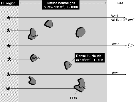
Figure 11: An illustration of the interface between the ionized gas of the H ii region and the surrounding neutral medium.

One usually models photodissociation regions (PDRs) as a single-interface H ii region/molecular cloud, and the material in the PDRs is generally assumed to be relatively uniform. However, on larger scales, the photodissociation front is likely to be rather clumpy, composed by small dense molecular clumps embedded in a more diffuse and mainly neutral medium. The PDRs are located on the surfaces of these clumps (Meixner & Tielens 1993). The clump distribution controls the far-UV photon penetration in the sense that the far-UV radiation passes between the dense clumps and is able to partially ionize the diffuse gas (see Fig. 11). According to the above-mentioned sketch, the ISM in NGC604 is probably quite complex and the absorption is likely to arise in different gaseous phases, i.e., diffuse ionized gas, diffuse neutral gas, or small dense H₂ clouds. However, the densest clouds are opaque to the far-UV radiation and do not contribute to the total UV spectrum. Moreover, we cannot see the direct contribution of the PDRs to the absorption spectrum, since the UV radiation generating these PDRs is blocked by the foreground associated dense molecular clouds. On the other hand, this contribution could manifest itself in scattered light, since dust is certainly present on the surfaces of the dense clumps (Maíz-Apellániz et al. 2004). However, the presence of scattered light has not yet been assessed. We thus expect the neutral absorption lines to arise mainly from the diffuse neutral gas in NGC604, with a possible contribution from the PDRs.

Table 9: Metal column densities in NGC604 from the LWRS and MDRS spectra (in logarithmic units of the column density in cm^-2), where errors are given at 2 $\sigma$, ’SF’ stands for the simultaneous fit method, ’IF’ stands for the independent fits (see Sect. 3.1), and ’LOSC’ stands for the line of sight cloud at $\sim-150$ km s^-1.

	NGC604	NGC604	NGC604	NGC604	LOSC	Galacticb
	LWRS, IF	LWRS, SF	MDRS, SF	”multi”a	LWRS, SF	LWRS, SF
N i	$15.31^{+0.34}_{-0.17}$	$15.14^{+0.02}_{-0.02}$	$15.26^{+0.06}_{-0.05}$	$[15.1,\gtrsim 16.0]$	$<12.31^{\mathrm{c}}$	$15.84$
O i	$16.52^{+0.19}_{-0.15}$	$16.26^{+0.05}_{-0.04}$	$16.40^{+0.34}_{-0.14}$	$[16.3,\gtrsim 17.0]$	$16.16^{+0.82}_{-0.46}$	$17.13$
Si ii	$15.54^{+0.11}_{-0.06}$	$15.52^{+0.04}_{-0.04}$	$15.62^{+0.10}_{-0.07}$	$[15.5,\gtrsim 16.5]$	$14.28^{+0.25}_{-0.36}$	$15.41$
P ii	$13.70^{+0.09}_{-0.08}$	$13.66^{+0.06}_{-0.07}$	$13.68^{+0.14}_{-0.15}$	$[13.7,14.0]$	$12.75^{+0.32}_{-0.58}$	$14.32$
Ar i	$13.86^{+0.07}_{-0.06}$	$13.95^{+0.04}_{-0.04}$	$14.06^{+0.07}_{-0.07}$	$[13.7,14.0]$	$<12.75^{\mathrm{c}}$	$14.21$
Fe ii	$14.89^{+0.03}_{-0.03}$	$14.88^{+0.02}_{-0.02}$	$14.94^{+0.04}_{-0.05}$	$[14.8,15.0]$	$14.51^{+0.15}_{-0.12}$	$14.95$

• Results from the multicomponent analysis are discussed in Sect. 9.

• Errors on the Galactic estimates are on the order of $\sim 0.15$ dex.

• Upper limits calculated at 2 $\sigma$.

In Table 9 we report the column densities inferred from the two FUSE observations with both methods, as explained in Sect. 3.1, i.e., independent fits (IF) for each element and simultaneous fit (SF) for several grouped elements. Determinations of Si ii, P ii, and Fe ii column densities, using the two approaches with the same LWRS spectrum, are consistent within the errors, while those of N i, O i, and Ar i are significantly different. The disagreement could be due to systematic errors introduced by the SF approach. This method assumes that species share temperatures, heliocentric velocities, and turbulent velocities. The errors associated to this assumption are not included in the uncertainties we mention.

The IF method was not used to determine column densities from the MDRS observation because of a signa-to-noise ratio too low that results in unstable solutions. Furthermore, the results from the two different observations (LWRS and MDRS apertures, SF method) do not in general agree with each other well. The inconsistencies could be explained by the different aperture sizes, together with the large extent of NGC604 cluster in the far-UV (see Sect. 2), or by the systematic effects discussed in the previous paragraph.

In their study of the diffuse molecular hydrogen content in M33, Bluhm et al. (2003) also derived O i, Ar i, and Fe ii column densities in NGC604 (and associated 1$\sigma$ errors) by using the curve-of-growth method based on the equivalent widths inferred from the same FUSE LWRS spectrum we analyzed. The authors obtained $16.20^{+0.30}_{-0.20}$ for O i, which is consistent with our LWRS, SF value, but significantly lower than the LWRS, IF value. Their derived Ar i column density, $13.65^{+0.15}_{-0.10}$, is also lower than our determinations. Finally, the estimate of the Fe ii column density, $15.00^{+0.10}_{-0.10}$, is only marginally consistent with our values.

7 Modelling the ionization structure with CLOUDY

In order to derive abundance ratios from column density measurements, it is generally assumed that the primary ionization state of one element is representative of its total abundance in the neutral gas. We expect to find all elements with larger ionization potential than that of hydrogen (13.6 eV) as neutral atoms in the H i gas. This is the case for N, O, and Ar, although some fraction of argon (and to a lesser extent nitrogen) can be singly ionized in low-density neutral regions, due to a large photoionization cross-section (Sofia & Jenkins 1998). Fe, P, and Si are mostly found as single-charged ions, with negligible amounts of neutral atoms. Thus N i, O i, Si ii, P ii, Ar i, and Fe ii should be the dominant forms of the respective elements in the neutral gas, and their column densities are thought to be representative of the abundances of the element.

However, ionization corrections may be needed since these atoms or ions can also exist in the ionized gas of the H ii region along the sightlines, contributing to the absorption lines we observe. In order to estimate this contamination, we modelled the ionized gas using the photoionization code CLOUDY (Ferland 1996; Ferland et al. 1998). We assumed that the H ii region is a homogeneous Strömgren sphere (with a radius $R_{s}$), ionized by a single star having the same radiation field as the stellar cluster. Although this is a very idealized situation, this is certainly sufficient for our purpose of obtaining rough estimates of the ionization corrections. The input N, O, Ar, and Fe abundances in the ionized gas are the observed abundances. They are taken from Esteban et al. (2002), which accounts for electronic temperature fluctuations and provides consistent abundances of these elements in the ionized gas from the same dataset. The input P and Si abundances are calculated assuming, respectively, that P/O is equal to the solar ratio (see Lebouteiller et al. 2005 for P/O measurements in the Milky Way) and that Si/O is equal to the mean value measured in the ionized gas of BCDs (Izotov et al. 1999). The hydrogen volumic density is from Melnick et al. (1980). We used two different stellar continua to constrain our models. In model (1), we use a stellar continuum built upon the observed flux at all wavelengths. Model (2) simply assumed a Kurucz stellar continuum at a temperature of 48 000 K.

Table 10: Optical emission-line intensities (normalized to $I$(H$\beta$)=100.0) given by the observations and by our models (see text).

Lines	H$\gamma$	H$\alpha$	$[$O iii$]$	$[$O iii$]$	$[$N ii$]$	$[$N ii$]$	He i	He i	He i
$\lambda$ (Å)	4340	6563	4959	5007	6548	6584	4471	6678	5876
NGC604, model (1)	47.1	291.2	90.3	260.9	11.4	33.6	4.1	3.3	11.7
NGC604, model (2)	47.0	294.0	81.8	236.2	10.0	29.7	4.2	3.4	12.1
NGC604, Esteban et al. (2002)	46.6	291.0	78.0	250.0	9.8	26.3	4.4	3.7	13.1
NGC604, Kwitter et al. (1981)	45.7	281.8	67.6	208.9	9.3	28.2	3.8	2.7	8.1
NGC604, Vilchez et al. (1988)	44.3	286.0	77.5	207.7	12.4	33.5	3.7	2.7	11.5
NGC5461	46.5	291.0	112.0	352.0	10.8	31.2	4.4	3.6	12.7
NGC5471	47.6	278.0	209.0	640.0	1.9	6.2	4.1	2.9	11.8
NGC2363	47.3	278.0	244.0	729.0	0.4	1.5	4.1	2.9	12.3

The resulting optical emission-line intensities obtained with both models are given in Table 10. For comparison, we report the values of three other giant H ii regions. It can be seen that some lines differ significantly for each object, allowing us to constrain the model. Results of the two models agree reasonably well with each other and with the observed intensities. From these models we calculated the relative ionization fractions of each species within the Strömgren sphere (see Fig. 12) and derived the expected column densities of N i, O i, Si ii, P ii, Ar i, and Fe ii in the ionized gas (assuming that half of the material is in front of the stellar cluster). These quantities are subtracted from the observed FUSE column densities in order to obtain the final column densities in the neutral gas alone (see column 3 of Table 11). The corrections are relatively small except for Si ii and P ii. This compares well with the findings of Aloisi et al. (2003) in IZw 18. The authors find that ionization effects are negligible for H, N, O, Ar, and Fe, the only exception being silicon.

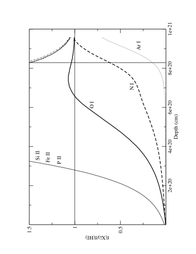
Figure 12: Ionization fraction of each species relative to H i, as a function of the distance to the ionizing source. O i, N i, and to some extent Ar i are well-coupled with H i in the neutral gas (i.e., for distances larger than $R_{s}=8.20\times 10^{20}$ cm, which is the radius of the Strömgren sphere).

Table 11: Abundances of N, O, Si, P, Ar, and Fe in the neutral gas, where IC stands for ionization correction (see Sect. 7) and errors are at $2\sigma$.

	Ion	IC (dex)	$\log$ (X/H)a	$[$X/H$]$	$[$X/H$]_{\rm HII}^{\mathrm{b}}$
N	N i	$-0.09$	$-5.70^{+0.30}_{-0.30}$	$-1.48^{+0.31}_{-0.31}$	$-0.32^{+0.32}_{-0.32}$
			$[-5.7,\gtrsim-4.8]$	$[-1.5,\gtrsim-0.6]^{\mathrm{c}}$
O	O i	$-0.08$	$-4.57^{+0.31}_{-0.31}$	$-1.23^{+0.32}_{-0.32}$	$+0.00^{+0.22}_{-0.22}$
			$[-4.5,\gtrsim-3.8]$	$[-1.2,\gtrsim-0.5]^{\mathrm{c}}$
Si	Si ii	$-0.34$	$-5.57^{+0.31}_{-0.31}$	$-1.08^{+0.35}_{-0.35}$	/d
			$[-5.6,\gtrsim-4.6]$	$[-1.2,\gtrsim-0.2]^{\mathrm{c}}$
P	P ii	$-0.15$	$-7.24^{+0.31}_{-0.32}$	$-0.60^{+0.33}_{-0.32}$	/d
			$[-7.2,\gtrsim-6.9]$	$[-0.6,-0.3]^{\mathrm{c}}$
Ar	Ar i	$-0.05$	$-6.85^{+0.31}_{-0.31}$	$-1.03^{+0.33}_{-0.33}$	$+0.25^{+0.20}_{-0.20}$
			$[-7.1,\gtrsim-6.8]$	$[-1.3,-1.0]^{\mathrm{c}}$
Fe	Fe ii	$-0.04$	$-5.91^{+0.30}_{-0.30}$	$-1.36^{+0.31}_{-0.31}$	$-1.02^{+0.22}_{-0.22}$
			$[-6.0,\gtrsim-5.8]$	$[-1.4,-1.2]^{\mathrm{c}}$

• Values derived from the simultaneous fit method using the FUSE LWRS spectrum (see Sect. 6.2), after respective ionization correction.

• Ionized gas abundances from Esteban et al. (2002).

• Values referring to the multicomponent analysis presented in Table 9 and discussed in Sect. 9.

• No direct abundance determinations exist in the ionized gas.

Note that we could not estimate the amount of species in higher ionization stages in the neutral gas. Indeed Ar i, and to a less extent N i, could be partly ionized into Ar ii and N ii in a low-density ISM, while hydrogen is still into H i. For this reason, we might underestimate the argon and nitrogen abundances in the neutral gas when using Ar i and N i for Ar and N. Depending on the hardness of the radiation field, Ar/H can be larger by $0.2$ up to $0.7$ dex than Ar i/H i (Sofia & Jenkins 1998). The situation is expected to be much less severe for N i, however.

8 Chemical abundances in the neutral and ionized gas

In Table 11 we report the abundances toward NGC604 in the neutral gas and, for comparison, in the ionized gas of the H ii region. For the latter we used abundances given in Esteban et al. (2002), instead of the older values from Kwitter et al. (1981) and Vilchez et al. (1988). This, because Esteban et al. homogeneously derived the N, O, Ar, and Fe abundances from a higher resolution optical spectrum, accounting for electronic temperature fluctuations. We estimate the Si abundance in the ionized gas by assuming that the abundance ratio Si/O is equal to the mean value measured in BCDs (Izotov et al. 1999). Abundances are normalized to the solar values from Asplund et al. (2004) as $[\textrm{X/H}]\leavevmode\nobreak\ =\leavevmode\nobreak\ \log\leavevmode\nobreak\ \textrm{(X/H)}\leavevmode\nobreak\ -\leavevmode\nobreak\ \log\leavevmode\nobreak\ \textrm{(X/H)}_{\odot}$. Figure 13 is a graphic representation of these data.

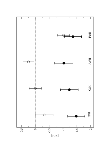
Figure 13: Abundances of N, O, Ar, and Fe in the neutral and ionized gas, compared to the solar values (from Asplund et al. 2004). We use the notation $[$X/H$]$ = $\log$ (X/H) $-$ $\log$ (X/H)_⊙. Empty circles are values for the ionized gas from Esteban et al. (2002). Filled circles indicate values in the neutral gas as determined from the simultaneous fit in the FUSE LWRS spectrum, using a single-component analysis. They may be underestimated for N, O, and Ar (see Sect. 9).

In the neutral gas the abundances of all heavy elements that we obtain are consistent within $2\sigma$ with the oxygen abundance, which is on the order of $1/10$ solar (see Table 11). If real (i.e., not driven by the large uncertainties in the H i column density), this consistency would be somewhat surprising, since we expect at least Si and Fe to be depleted onto dust grains. Indeed, the medium we are considering should be comparable to the diffuse neutral medium in front of stars like $\zeta$ Ophiuchi or $\mu$ Colombae in our own Galaxy. N, O, P, and Ar are not depleted or only a little (within a factor less than $\sim 3$) toward these Galactic sightlines, while Si and Fe show depletions by a factor of at least $\sim 3$ and 10, respectively (Savage & Sembach 1996; Snow & Witt 1996; Howk, Savage & Fabian 1999). In a similar way, the heavy element abundances in the ionized gas of the H ii region are also consistent within the errors with the O abundance, which is solar in this case. The only exception is the gaseous Fe, which is about $1/10$ solar.

If real, the observed abundance trends indicate that nitrogen, oxygen, and argon are lower by $\gtrsim 1$ dex in the neutral gas phase as compared to the ionized one. This confirms a similar trend already observed in blue compact dwarf galaxies, and it contrasts with the most recent finding of no offset in the $\alpha$-element content of the neutral and ionized gas in the nearby damped Lyman-$\alpha$ galaxy SBS 1543+593 (Bowen et al. 2005). Ionization corrections in the neutral medium cannot fully explain the similar offsets of N, O, and Ar in NGC604, since Ar is expected to be much more affected than N and O (Sect. 7).

Iron is instead the only element showing similar abundances in the two gaseous phases. The iron behavior requires that this element has the same gas abundance and depletion factor in both the neutral and ionized gas phases. This is rather surprising, because we expect iron to be underabundant in the H i region and depletion on grains to be similar or larger in the neutral medium compared to the H ii region (but see Sect. 9).

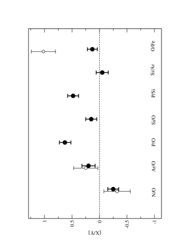
Figure 14: Abundance ratios in the neutral and ionized gas of NGC604. See Fig. 13 for a description of the plot. The abundances in the neutral gas weres determined using a single-component model.

For what concerns the relative abundance ratios, we observe the following behaviors (see Fig. 14). The $\alpha$-elements O, Si, and Ar are roughly in solar proportion in both the neutral and the ionized ISM. This seems to indicate that Ar does not suffer from the ionization effects typical of a low-density neutral medium (see Sect. 7) and that Si is not more depleted in the H i gas than in the H ii gas, another rather surprising result. In a similar way, the consistency of the (subsolar) abundance ratio N/O in both the neutral and ionized gas suggests that N is affected neither by ionization nor by depletion effects. The behavior of phosphorus in the neutral gas is also particularly intriguing, since P/O and P/Si in this gas seem to be super-solar, in disagreement with what found by Lebouteiller et al. (2005): these authors derived essentially solar P/O ratios for several sightlines sampling the Galactic diffuse ISM, as well as for a few damped Lyman-$\alpha$ systems and the ISM of the small Magellanic cloud toward the star Sk108.

We show in the next section that the N i, O i, and Si ii column density determinations may be severely affected by saturation of hidden velocity components. If this is indeed the case, the analysis of Sect. 6, which assumes a single absorbing neutral component with a large velocity dispersion in front of NGC604, would result in an underestimate of the abundances of these elements. Once hidden saturation is properly taken into account, it is possible to easily reconcile all the puzzling results from the behavior of the various heavy elements in a very simple way, i.e., by considering the possibility that the neutral and ionized gas could have similar abundances.

9 Multicomponent analysis

Instead of arising from a single neutral cloud with a large velocity dispersion, the interstellar lines we detect might be the blend of many unresolved absorption components whose widths and velocities are related to the ISM structure and to the source morphology. As we now show, this may result in a severe underestimate of the column densities for the most saturated lines if a single-component analysis is made. It is not possible with the present data to assess whether multiple saturated components contribute to the absorption lines we observe. However, it is possible to perform empirical tests and to calculate the uncertainties associated with the presence of multiple $-$ possibly saturated $-$ components. A detailed analysis can be found in Lebouteiller (2005). In this section, we summarize the method and the results.

9.1 Presence of hidden saturated components

To identify which lines can suffer from hidden saturation, we first consider the presence of a test component placed at various velocities within the broad line. We choose for this component a $b$-value of $2$ km s^-1, which we consider as the minimum value allowed for a single sightline intersecting a single interstellar cloud (Tumlinson et al. 2002 measured $b$ values systematically larger than $1.6$ km s^-1 toward stars of the Magellanic Clouds).

Among the detected lines in NGC604, Fe ii $\lambda 1142$ is the only one for which the test component can never be saturated due to the relatively low value of the oscillator strength. The other lines of Fe ii and all the lines of the other species could suffer from hidden saturation by a component with $b$ = $2$ km s^-1. Hence, the column density derived from the observed global $\lambda 1142$ Fe ii line should not be affected by the systematic errors associated with hidden saturated components, even in the center of the global line, where the optical depth is maximum. Note that it can still suffer from uncertainties due to the non-linear sum of the individual spectra (see previous section). The Fe ii column density obtained using the $\lambda 1142$ line alone is $\log N(\textrm{Fe\,{\sc ii}})=14.97\pm 0.07$, slightly higher than the value we found earlier using all the available lines ($14.88^{+0.02}_{-0.02}$, see Sect. 6.2). This confirms that using stronger Fe ii lines in addition to $\lambda 1142$ introduces systematic errors if there are hidden saturated components. However, the errors do not exceed $\sim 0.1$ dex in the case of Fe ii.

For other species, we cannot rule out that even their weakest observable lines could be made of saturated individual components. Although we have no information on the actual velocity component distribution responsible for the global profile, it is still possible to test various plausible distributions, which can somehow be constrained if we simultaneously adjust and fit all the lines of a given species, from the weakest line to the heavily saturated one.

9.2 Test of possible component distributions

We consider here various component distributions, fully defined by the number of components $n_{c}$, by the turbulent velocity $b$ of each component, and by the spacing ${\Delta}V$ between them (which can possibly be lower than $b$, depending on the number of components).

The ideal species to test for plausible distributions is Fe ii because of the large number of lines available, with a wide range of oscillator strengths. Fe ii might have a space distribution differing slightly from that of the other species, due to abundance and ionization inhomogeneities. However, here we only wish to test the method, so we ignore this problem.

We consider various distributions with $n_{c}$ varying between 1 and 20 and $b$ between 2 and 44 km s^-1 (which is the highest $b$ value for a single component, see Sect. 6.1), while ${\Delta}V$ is set so that the components are uniformly distributed within the observed Fe ii line widths. For a given line, the column densities in each component are considered as free parameters by the fitting procedure Owens.

We find that many component distributions provide a $\chi^{2}$ equal to or lower than the $\chi^{2}$ for a single-absorption component. We thus consider all these distributions as mathematically and physically plausible. The distributions give a total column density (sum of all the components) in agreement within 0.1 dex with the determination using a single component. Furthermore, we notice that satisfactory distributions implying components with low $b$ values (potentially responsible for saturation effects) also imply a large number of components $n_{c}$, so that the total column density is dispersed in many components with relatively low column densities. Typically, at least 13 components with $b=2$ km s^-1 were needed to adjust the lines. We do not find satisfactory distributions implying high column densities together with low $b$-values.

We used the velocity distributions that we found satisfactory to fit the Fe ii lines, to also fit the lines of the other species (N i, O i, Si ii, P ii, and Ar i). We discovered that the distributions do not introduce strongly saturated components in the P ii and Ar i lines, even when $b=2$ km s^-1. The column density we determined using the velocity distributions is similar to the estimate using a single-component fit within $\sim 0.2$ dex. However, several possible distributions imply that even the weakest N i, O i, and Si ii lines are made of saturated components. For these species, the sum of the column densities in the individual components can be larger than $2-3$ dex in comparison with the result of the single-component analysis.

Thus the column densities of N i, O i, and Si ii could be severely underestimated. On the other hand, the Fe ii and, to a lesser extent, the P ii and Ar i lines do not seem to be strongly affected by systematic errors due to the presence of hidden saturated components. We show the ranges of column densities derived from the multicomponent analysis in Table 9.

Focussing on the P ii, Ar i, and Fe ii column densities only, the interpretation of the abundances in the neutral gas differs from what is discussed in Sect. 8. Iron has similar abundances in the ionized and neutral phases, suggesting that the two gaseous phases could indeed have similar metallicities. The underabundance of Ar i could then be explained by the fact that argon can be partly ionized into Ar ii in this gaseous phase. The actual Ar/H would be closer to Ar ii/H i. This result would agree with the findings in IZw36 (Lebouteiller et al. 2004). Finally, little can be said about the abundances of N i, O i, and Si ii, which could well be similar to those in the H ii region. To conclude, the evidence of a difference in abundances in the H i and in the H ii gases essentially vanishes as a result of our tests.

10 Conclusion

This study provides the first detailed analysis of interstellar lines of H i, N i, O i, Si ii, P ii, Ar i, and Fe ii in the neutral medium in front of a giant H ii region in the spiral galaxy M33. Since NGC604 is a nearby system, we have been able to perform the necessary critical tests for analyzing possible selection effects.

• In the frame of a simple model, we have derived column densities of metals in the neutral gas of NGC604 from both FUSE LWRS and MDRS spectra. These independent estimates allowed us to quantify the effects of the source extent on the interstellar absorption line profiles.

• The continuum used for the profile fitting was checked by comparison with a theoretical stellar model. Besides, no significant contamination from stellar photospheric lines was found for the H i absorption lines we investigated.

• A particular attention was given to the neutral hydrogen column-density determination. The Ly$\beta$ line from the FUSE LWRS and MDRS spectra is contaminated by the O vi P Cygni doublet. We modelled this contamination to obtain the H i column density. Also, profile fitting of the Ly$\alpha$ absorption in HST/STIS spectra toward individual stars in the cluster NGC604 reveals inhomogeneities in the neutral gas. We finally adopted the FUSE value of $\log\leavevmode\nobreak\ N$(H i)=20.75 with a conservative error of $\pm$0.3 dex to account for all the possible uncertainties. Within the errors, this H i column density is consistent with the IUE determination using Ly$\alpha$ and with the 21 cm line radio observations.

• By modelling the ionization structure of the H ii gas with the photoionization code CLOUDY, we have shown that N i, O i, Ar i, and Fe ii are reliable tracers of the neutral gas, in contrast with Si ii and P ii, which require ionization corrections to obtain final abundances in the neutral phase.

Adjusting absorption lines with a single component, we find that N, O, Ar, and Si are underabundant in the neutral gas as compared to the ionized gas by factors $\gtrsim 10$, while Fe/H is similar in the two gaseous phases. This result is rather puzzling, since iron is expected to be equally or more depleted in grains in the neutral gas compared to the ionized one, and there is no reason it should be relatively more abundant in the neutral gas.

This led us to investigate in detail the influence of individual unresolved components in the analysis of absorption lines. Using the method and results of Lebouteiller (2005), we argue that N i, O i, and Si ii column densities can be severely underestimated if there are saturated hidden components, while Fe ii and, to some extent, Ar i and P ii should be more reliably determined. Since Fe is the only element to show similar abundances in the neutral and ionized gas, it is possible that all elements indeed have similar abundances in both media. The underabundance of Ar would then be due to the fact that we used Ar i/H i to estimate Ar/H, when (Ar i+Ar ii)/H i should be used instead.

- (1) Aloisi, A., Savaglio, S., Heckman, T. M., et al. 2003, ApJ, 595, 760
- Asplund et al. (2004) Asplund M., Grevesse N., Sauval J. 2004 ASP conf. series, in press
- (3) Bluhm, H., de Boer, K. S., Marggraf, O., Richter, P., & Wakker, B. P. 2003, A&A, 398, 983
- Bohlin et al. (1978) Bohlin, R. C., Savage, B. D., & Drake, J. F. 1978, ApJ, 224, 132
- Bowen et al. (2005) Bowen, D. V., Jenkins, E. B., Pettini, M., & Tripp, T. M. 2005, ApJ, 635, 880
- (6) Cannon, J. M., McClure-Griffiths, N. M., Skillman, E. D., & Côté, S. 2004, ApJ, 607, 274
- (7) Churchwell, E., & Goss, W. M. 1999, ApJ, 514, 188
- (8) Deul, E. R., & van der Hulst, J. M. 1987, A&AS, 67, 509
- (9) Dickey, J. M., & Brinks, E. 1993, ApJ, 405, 153
- (10) Dodorico, S., & Rosa, M. 1981, ApJ, 248, 1015
- (11) Drissen, L., Moffat, A. F. J., & Shara, M. M. 1993, AJ, 105, 1400
- Dunne et al. (2003) Dunne, L., Eales, S., Ivison, R., Morgan, H., & Edmunds, M. 2003, Nature, 424, 285
- (13) Esteban, C., Peimbert, M., Torres-Peimbert, S., & Rodríguez, M. 2002, ApJ, 581, 241
- (14) Ferland, G. J., Korista, K. T., Verner, D. A., et al. 1998, PASP, 110, 761
- (15) Ferland, G. J. 1996, Hazy, a Brief Introduction to CLOUDY 90, Univ. of Kentucky Physics Department Internal Report
- (16) Freedman, W. L., Wilson, C. D., & Madore, B. F. 1991, ApJ, 372, 455
- (17) Gonzalez Delgado, R. M., Leitherer, C., & Heckman, T. 1997, ApJ, 489, 601
- Gray & Edmunds (2004) Gray, M. D., & Edmunds, M. G. 2004, MNRAS, 349, 491
- (19) Hébrard, G., Lemoine, M., Vidal-Madjar, A., et al. 2002, ApJS, 140, 103
- (20) Heckman, T. M., Sembach, K. R., Meurer, G. R., et al. 2001, ApJ, 554, 1021
- Heiles (1975) Heiles, C. 1975, A&AS, 20, 37
- (22) Hobbs, L. M. 1974, ApJ, 191, 395
- Hollenbach & Tielens (1999) Hollenbach, D. J., & Tielens, A. G. G. M. 1999, Reviews of Modern Physics, 71, 173
- (24) Hoopes, C. G., Sembach, K. R., Heckman, T. M., et al. 2004, ApJ, 612, 825
- (25) Howk, J. C., Savage, B. D., & Fabian, D. 1999, ApJ, 525, 253
- (26) Israel, F. P., & Kennicutt, R. C. 1980, Astrophys. Lett., 21, 1
- (27) Israel, F. P., & van der Kruit, P. C. 1974, IAU Symp. 60: Galactic Radio Astronomy, 60, 227
- (28) Izotov, Y. I., & Thuan, T. X. 1999, ApJ, 511, 639
- (29) Jenkins, E. B. 1986, ApJ, 304, 739
- (30) Kunth, D., & Sargent, W. L. W. 1986, ApJ, 300, 496
- (31) Kunth, D., Lequeux, J., Sargent, W. L. W., & Viallefond, F. 1994, A&A, 282, 709
- (32) Kwitter, K. B., & Aller, L. H. 1981, MNRAS, 195, 939
- (33) Lebouteiller, V., Kunth, D., Lequeux, J., et al. 2004, A&A, 415, 55
- (34) Lebouteiller et al. 2005, A&A, 443, 509
- (35) Lebouteiller 2005, PhD University Pierre et Marie Curie, Paris
- (36) Lecavelier des Etangs, A., Désert, J.-M., Kunth, D., et al. 2004, A&A, 413, 131
- (37) Leitherer, C., Schaerer, D., Goldader, J. D., et al. 1999, ApJS, 123, 3
- (38) Lemoine, M., Vidal-Madjar, A., Hébrard, G., et al. 2002, ApJS, 140, 67
- Maiolino et al. (2004) Maiolino, R., Schneider, R., Oliva, E., Bianchi, S., Ferrara, A., Mannucci, F., Pedani, M., & Roca Sogorb, M. 2004, Nature, 431, 533
- (40) Maíz-Apellániz, J., Pérez, E., & Mas-Hesse, J. M. 2004, AJ, 128, 1196
- (41) Martin, C. L., Kobulnicky, H. A., & Heckman, T. M. 2002, ApJ, 574, 663
- Meixner & Tielens (1993) Meixner, M., & Tielens, A. G. G. M. 1993, ApJ, 405, 216
- (43) Melnick, J. 1980, A&A, 86, 304
- (44) Miskey, C. L., & Bruhweiler, F. C. 2003, AJ, 125, 3071
- (45) Moos, H. W., Cash, W. C., Cowie, L. L., et al. 2000, ApJ, 538, L1
- (46) Newton, K. 1980, MNRAS, 190, 689
- Pellerin (2006) Pellerin, A. 2006, AJ, 131, 849
- (48) Pettini, M., & Lipman, K. 1995, A&A, 297, L63
- (49) Robert, C., Pellerin, A., Aloisi, A., et al. 2003, ApJS, 144, 21
- (50) Savage, B. D., & Sembach, K. R. 1996, ARA&A, 34, 279
- (51) Snow, T. P., & Witt, A. N. 1996, ApJ, 468, L65
- Sofia & Jenkins (1998) Sofia, U. J., & Jenkins, E. B. 1998, ApJ, 499, 951
- (53) Tenorio-Tagle, G. 1996, AJ, 111, 1641
- (54) Tenorio-Tagle, G., Muñoz-Tuñón, C., Pérez, E., Maíz-Apellániz, J., & Medina-Tanco, G. 2000, ApJ, 541, 720
- (55) Thuan, T. X., Lecavelier des Etangs, A., & Izotov, Y. I. 2002, ApJ, 565, 941
- (56) Thuan, T. X., Lecavelier des Etangs, A. 2005 in press
- (57) Viallefond, F., Boulanger, F., Cox, P., et al. 1992, A&A, 265, 437
- (58) Velden, L. 1970, IAU Symp. 38: The Spiral Structure of our Galaxy, 38, 164
- Vidal-Madjar et al. (2000) Vidal-Madjar, A., et al. 2000, ApJ, 538, L77
- (60) Vilchez, J. M., Pagel, B. E. J., Diaz, A. I., Terlevich, E., & Edmunds, M. G. 1988, MNRAS, 235, 633
- (61) Wilson, C. D., & Matthews, B. C. 1995, ApJ, 455, 125