Time resolved spectroscopy of GRB 021004 reveals a clumpy extended wind

Abstract

High resolution spectroscopy of GRB 021004 revealed a wealth of absorption lines from several intermediate ionization species. The velocity structure of the absorber is complex and material with velocity up to $\lower 2.15277pt\hbox{$\;\buildrel>\over{\sim}\;$}3000$ km s^-1 is observed. Since only the blueshifted component is observed, the absorber is very likely to be material closely surrounding the gamma-ray burst. We use a time-dependent photoionization code to track the abundance of the ions over time. Thanks to the presence of absorption from intermediate ionization states at long times, we can estimate the location and mass of the components of the absorber. We interpret those constraints within the hypernova scenario showing that the mass loss rate of the progenitor must have been $\sim 10^{-4}\,M_{\odot}$ per year, suggestive of a very massive star. In addition, the wind termination shock must lie at a distance of at least $100$ pc, implying a low density environment. The velocity structure of the absorber also requires clumping of the wind at those large distances.

1 Introduction

The high luminosity of gamma-ray burst afterglows makes them ideal sources to probe their surrounding environment through absorption lines in their powerlaw, generally featureless spectra. In particular, time variability (or lack thereof) in the equivalent width of absorption lines can be used to constrain the size and density of the absorbing region surrounding the burst (Perna & Loeb 1998).

The association of GRBs with the collapse of massive stars (Stanek et al. 2003; Hjorth et al. 2003) makes absorption studies particularly useful as a new way to probe star-forming regions at intermediate and high redshifts and/or the last hundreds of years of the progenitor evolution. Lines associated with the material expelled by the star allow one to probe the velocity structure and metal content of the ejecta. The high quality and well sampled temporal evolution of the spectroscopic data gathered for GRB 021004 (Moeller et al. 2002; Matheson et al. 2003; Mirabal et al. 2003; Schaefer et al. 2003; Fiore et al. 2005; Starling et al. 2005) allows us for the first time to perform a detailed analysis.

GRB 021004 was detected by HETE II and an optical afterglow was detected within 10 minutes with an R-band magnitude of 15.34 (Fox et al. 2002). Superimposed on the standard power-law decay, the optical light curve shows several bumps (Holland et al. 2003), which can be interpreted either as density fluctuations (Lazzati et al. 2002; Heyl & Perna 2003), continuous activity of the inner engine or inhomogeneities in the fireball energy content (Nakar, Piran & Granot 2003). High resolution spectroscopy of the optical afterglow was reported by Fiore et al. (2005). Low-to-intermediate resolution spectroscopy was reported by Moeller et al. (2003), Mirabal et al. (2003), Matheson et al. (2003), Schaefer et al. (2003) and Starling et al. (2005). These observations revealed a large set of absorption lines spanning a velocity range of about $3000$ km s^-1 toward the observer. This is the only burst to date for which such high-velocity lines have been detected. The possibility of observing such an absorption system due to chance alignment of different absorbers was discussed and ruled out in previous work (see Schaefer et al. 2003; Mirabal et al. 2003; Fiore et al. 2005). Interpreted as absorption from the local GRB environment, the results of the spectroscopic follow-up studies are controversial. Starling et al. (2005) conclude that the lines must be coming from a fossil stellar wind with hydrogen enrichment from a companion. Mirabal et al. (2003) and Schaefer et al. (2003) attribute the lines to shells of material present around the progenitor. They also allow for the possibility of clumping. Neither of those studies took adequately into account the effect of the flash ionization of the burst photons on the environment.

High resolution spectroscopy ($R\sim 50000$) was obtained by Fiore et al. (2005). Several narrow components were resolved down to a width of a few tens of km s^-1, showing that some of the components observed at low resolution are in fact due to blending of finer velocity structures. Fiore et al. (2005) derived physical parameters for the absorbing medium modeling the ionization ratios with the code CLOUDY, which assumes ionization equilibrium. They obtained fairly constant ionization parameters for the different absorbers. They concluded that the absorber is stratified as a wind, since a $n\propto{}r^{-2}$ profile gives a constant ionization parameter over a broad range of distances. However, due to the highly time-dependent nature of the ionizing flux and the long recombination times with respect to the ionization times, their conclusions should be taken with caution. In this paper we combine all the available spectroscopic data and adopt a time-dependent photoionization code (Perna & Lazzati 2002) to determine the physical conditions of the absorber.

This paper is organized as follows: in $\S$2 we discuss the spectra of GRB 021004 and show that there is moderate evidence of time-variability in the equivalent width (EW) the observed CIV line. In $\S$3 we present our model for the light curve of GRB 021004 while the code and the data modeling technique are discussed in $\S$4 together with the results of the fit. We finally discuss our findings in $\S$5.

2 Spectrum of 021004

Figure 1: A portion of the high resolution spectrum of GRB 021004 (Fiore et al. 2005) showing the complex absorption from CIV ions. The two high velocity systems $A$ and $B$ discussed in the text are shown.

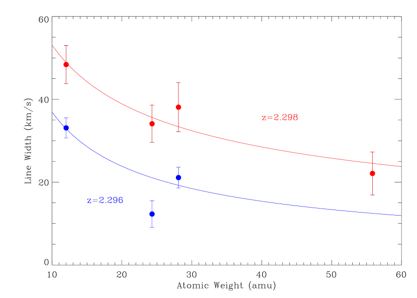
Figure 2: Line widths vs. ion mass for absorption lines in the $A$ and $B$ systems. Lines show fits with a thermal broadening model, which is statistically consistent with the data.

Fiore et al. (2005) were able to identify six absorption systems in the spectrum of GRB 021004 (see Fig. 1 of Fiore et al. 2005). These are characterized by the following velocities with respect to the Ly$\alpha$ emission frequency which sets the reference frame of the host galaxy ($z=2.328$): $v=0$ km s^-1 ($z=2.328$); $v\simeq-140$ km s^-1 ($z=2.328$); $v\simeq-220$ km s^-1 ($z=2.328$); $v=\simeq-630$ km s^-1 ($z=2.321$); $v\simeq-2730$ km s^-1 ($z=2.298$); $v\simeq-2900$ km s^-1 ($z=2.296$). The four low velocity systems are characterized by higher column densities and severely saturated line cores which prevent a robust measurement of the column density of the relative ions. They can be explained in the framework of a wind environment as absorption from material in the unshocked and shocked molecular cloud and/or from a previous stage of mass ejection from the progenitor star (Van Marle et al. 2005). We here concentrate on the two high velocity absorbers, characterized by velocities of order $3000$ km s^-1 that we call system $A$ and system $B$ (see Fig. 1). The analysis of the line widths of ions with different masses also shows that these two systems are simple, their width being due to thermal motions of the ions rather than to an underlying fine velocity structure (Fig. 2). The derived temperatures are: $T=1\times 10^{6}$ K ($z=2.298$); $T=3\times 10^{6}$ K ($z=2.296$). Throughout this paper we focus on the absorption of the CIV doublet $1550+1548$ Å and of the SiIV line at $1393$ Å.

In order to explore possible variations of the equivalent widths of these lines with time, we compiled all the data available in the literature (see above for references). The CIV data (which have larger signal to noise ratio than SiIV) are shown in Fig. 3. A fit with a constant yields $EW(t)=EW_{0}=1.59\pm 0.03$ with a $\chi^{2}/d.o.f.=26.6/12$. To test for variability we model the EW evolution with a linear function $EW(t)=EW_{0}+EW_{1}\,t$. We obtain $EW_{0}=1.67\pm 0.05$ and $EW_{1}=(-8.05\pm 3.20)\times 10^{-7}$ with $\chi^{2}/d.o.f.=20.3/11$. An F-test shows moderate evidence of variability at the $90\%$ level. Data have been taken with different telescopes and spectral resolutions. To test weather this may cause a spurious evolution of the EW, we show in the bottom panel of Fig. 3 the resolution with which each spectrum was taken. The absence of any clear trend makes us more confident of the reality of the detection of evolution in the CIV EW.

Figure 3: The equivalent width of the CIV doublet taken from the literature vs. time of observation. The best fit constant and time-variable models are overlaid (see text for more details). The F-test shows that the time-variable model provides a better description of the data at the $90\%$ confidence. The lower panel shows the resolutions of the spectra from which the EW measurement has been taken. They appear to be uncorrelated with time.

3 Models

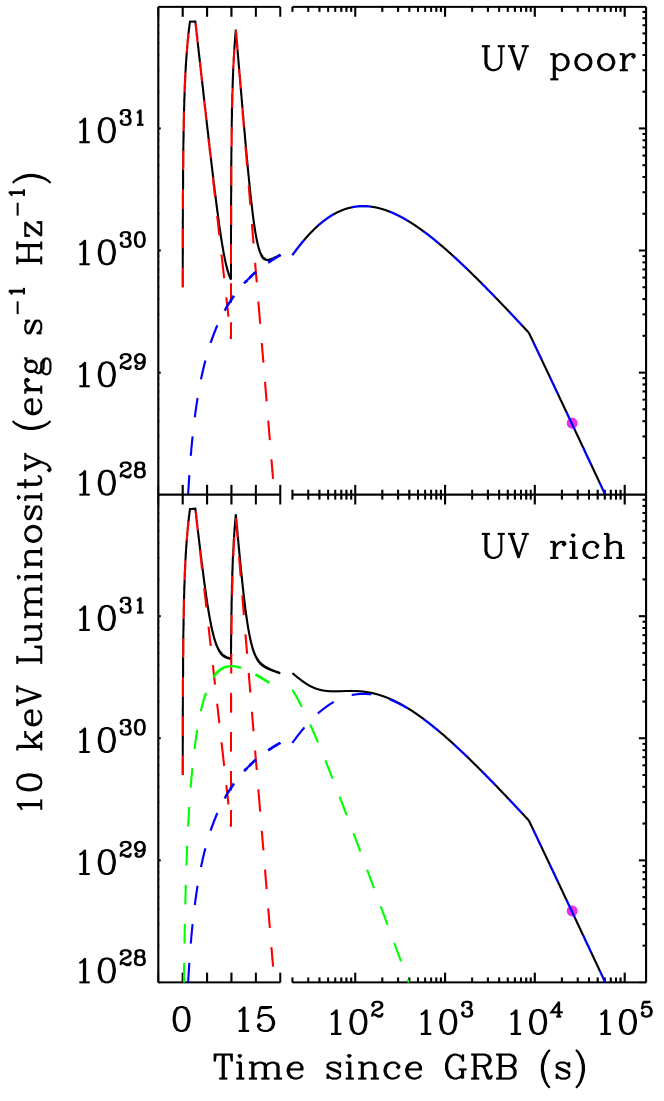
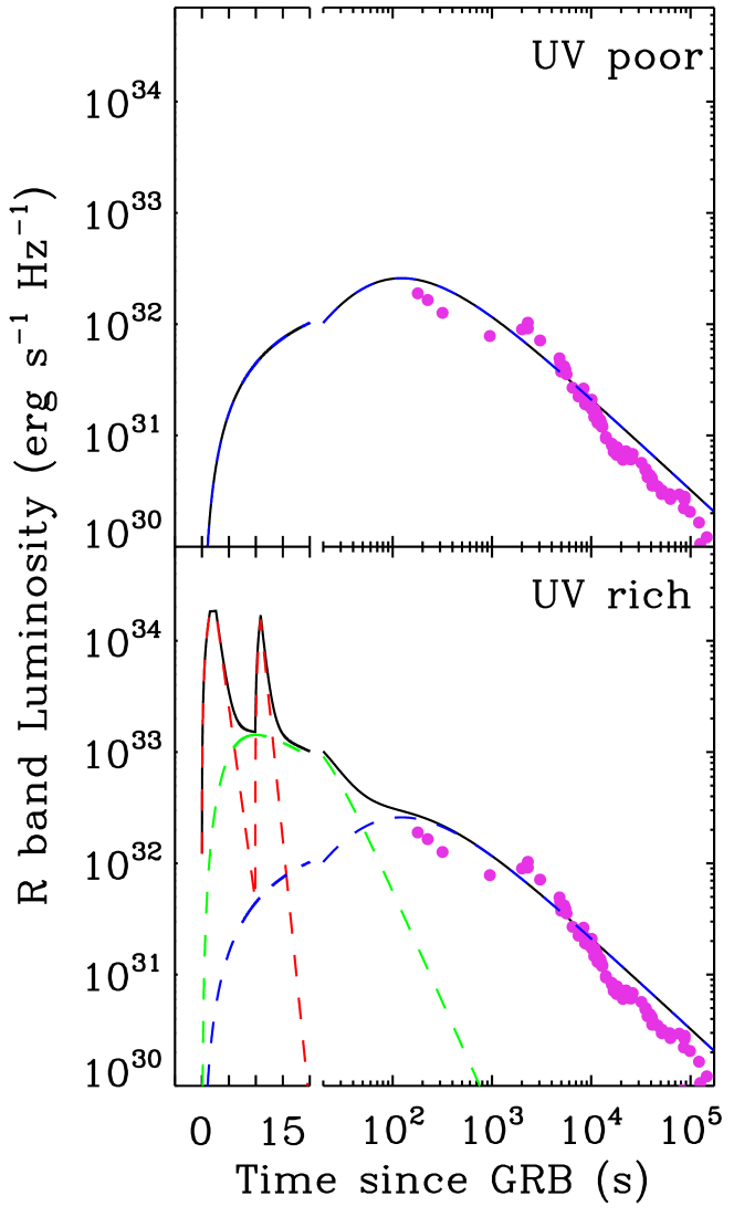
Figure 4: Left: X-ray (10 keV observed) light curve of GRB 021004 and its afterglow according to the model described in the text. Note that the first 20 seconds of the time scale are linear while the final ones are in logarithm. The top panels show the model with less UV radiation in the prompt and optical flash phases among those explored. The lower panels show the other extreme: a model in which the UV component is emphasized as much as the optical and X-ray constraints allow. The UV fluence is in all models dominated by the afterglow component and therefore the results differ only marginally between these two extremes. Right: Same as in the left panel but for the R-band.

We model the light curve of GRB 021004 with three components: the prompt phase, the afterglow and a possible optical flash.

The prompt phase is modeled with two pulses with a power-law spectrum (Barraud et al. 2003):

$$L(\nu,t)=4\times 10^{44}\,\nu^{-0.64}\,A(t)\qquad{\rm erg~{}s}^{-1}{\rm~{}Hz}^{-1}$$ (1)

where $A(t)=A_{1}(t)+A_{2}(t)+A_{3}(t)+A_{4}(t)+A_{5}(t)$:

$$A_{1}(t) = 0.157\,t\,\chi_{[0,1.5)}$$

$$A_{2}(t) = 0.235\,\chi_{[1.5,2.6)}$$

$$A_{3}(t) = 0.235\,e^{-{{t-2.6}\over{1.22}}}\,\chi_{[2.6,\infty)}$$ (2)

$$A_{4}(t) = (0.2\,t-1.98)\,\chi_{[9.9,10.9)}$$

$$A_{5}(t) = 0.2\,e^{-{{t-10.9}\over{0.9}}}\,\chi_{[10.9,\infty)}$$

where $\chi_{(a,b)}$ is the characteristic function of the interval $(a,b)$ ($\chi_{(a,b)}=1$ if $a<x<b$ and 0 otherwise). The normalization constant in Eq. 1 is chosen in such a way that $\int\,L\,dt\,d\nu=2\times 10^{52}$ erg in the $[7-400]$ keV band (Lamb et al. 2002). Given the lack of spectral information below $7$ keV observed ($23.2$ keV comoving), we allow for the possibility of a sharp break in the spectrum at this frequency, with $L(\nu)\propto\nu^{2}$ below $23.2$ keV.

The afterglow component (AG) is modeled with a broken power-law both for the temporal and spectral components. We model the afterglow spectral evolution in the framework of a fireball expanding in a homogeneous medium (Lazzati et al. 2002, but see Li & Chevalier 2003) with a power-law slope $p=2.1$ of the relativistic electron distribution (e.g. Holland et al. 2003). We obtain:

$$L(\nu,t)=5\times 10^{32}{{2\,t_{0}^{\alpha}}\over{\left(t^{0.3\alpha}+t_{0}^{0.3\left(\alpha-\beta\right)}\,t^{0.3\beta}\right)^{1/0.3}}}\,F(\nu,t)$$ (3)

where $t_{0}=43.2$ s, $\alpha=-2$, $\beta=0.825$ and

$$F(\nu,t)=\left\{\begin{array}[]{ll}\left({{\nu}\over{\nu_{0}}}\right)^{-0.55}&\nu<\nu_{B}(t)\\ \left({{\nu_{B}}\over{\nu_{0}}}\right)^{0.5}\left({{\nu}\over{\nu_{0}}}\right)^{-1.05}&\nu\geq\nu_{B}(t)\end{array}\right.$$ (4)

where

$$\nu_{B}(t)=2.5\times 10^{17}\,t^{-3/2}$$ (5)

and the time is in seconds.

In addition to the prompt and afterglow components, we allow for the presence of an optical flash (OF), as observed in GRB 990123 (Akerlof et al. 1999). In the case of GRB 021004, optical observations at such early times were not performed and the only constraints we have on reverse shock emission come from the fact that it could only marginally contribute to the afterglow at $t\lower 2.15277pt\hbox{$\;\buildrel>\over{\sim}\;$}600$ s (see also Kobayashi and Zhang 2003). We model the OF as (e.g. Draine & Hao 2002):

$$L(\nu,t)=2.2\times 10^{41}{{\left({{t}\over{t_{0}}}\right)^{2}}\over{\left[1+\left({{t}\over{t_{0}}}\right)^{2}\right]^{2}}}\left\{\begin{array}[]{ll}\nu^{-0.5}&\nu<\nu_{B}\\ \nu_{B}^{0.7}\,\nu^{-1.2}&\nu\geq\nu_{B}\end{array}\right.$$ (6)

where $\nu_{B}=8\times 10^{17}$ Hz.

While the afterglow is well constrained by the data, there is the possibility of a break in the prompt phase and there may be an optical flash. We therefore initially considered four different models. The two extreme versions, with the smallest flux in the optical-UV and with the highest flux in the optical-UV, are shown and compared to the observed photometry in Fig. 4. Even though the models in the figure look quite different, the optical-UV fluence is very similar since it is dominated by the late afterglow component, for which the spectrum is well constrained by the photometric data. Indeed, by running test fits, we confirmed that the characteristics of the absorber depend only marginally on the adopted spectral model. Therefore we concentrated the detailed analysis only on one model, the UV-poor one (upper panels of Fig. 4).

3.1 The absorber geometry

We explore two different geometries for the spatial distribution of the absorber. Given the high velocity of the absorber, it must be located in the unshocked part of the wind of the progenitor star. Therefore we first model our absorber as a smooth wind with density profile $n(R)\propto R^{-2}$. This model is characterized by two fitting parameters: the mass loss rate $\dot{M}$ in units of solar masses per year and the wind termination shock $R_{\rm{sh}}$ in parsec. The presence of structure in the velocity of the absorber suggests that the wind is clumped. We explore this possible geometry as follows. Given the fact that our computations are line-of-sight, we consider a thin shell geometry (with $\Delta R=0.1R$). This geometry is relevant if the clumps completely dominate the mass distribution. The model is characterized by two fitting parameters: the shell radius $R$ and the hydrogen column density $N_{H}$. Since the recombination times of free electrons onto ions are much longer than the times considered in the computation, we are insensitive to the density of free electrons. As a consequence, fixing a shell width does not imply any loss of generality.

The composition of the absorber is either a pure gas or a Milky Way like interstellar material, with a dust component. The metallicity can be varied as a free parameter. The dust component is a mixture of graphite and silicates (Mathis, Rumpl & Nordsieck 1977) with a size distribution

$$\frac{dn_{i}}{da}=A_{i}n_{H}a^{-\beta}$$ (7)

where $\beta=3.5$ (Mathis et al. 1977) in the range $a_{min}\simeq$ 0.005 $\mu$m, $a_{max}\simeq$ 0.25 $\mu$m. Given the data quality we did not deem it worth pursuing a deeper investigation allowing for different dust distributions.

Since the initial temperature of the absorbing material is not known, we explored a range of temperatures $10^{3}<T_{0}<10^{5}$ K. The upper limit represents the photospheric temperature of a massive WR star. We considered also lower temperatures since the wind cools adiabatically as it moves away from the star. We find that the late time ion populations are insensitive to the initial temperature $T_{0}$ for $T_{0}\lower 2.15277pt\hbox{$\;\buildrel<\over{\sim}\;$}10^{4}$ K (see Table 3).

4 Methods and results

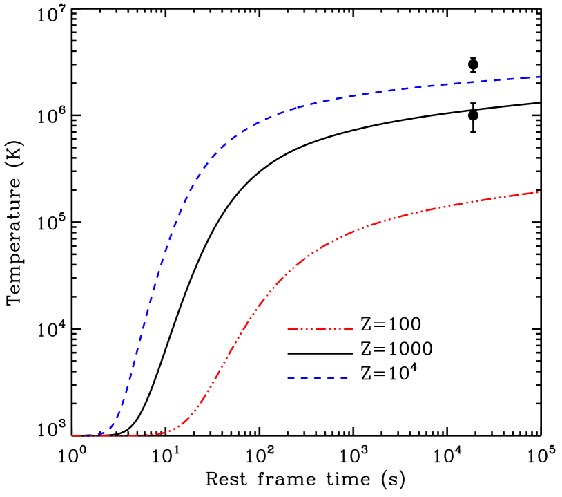
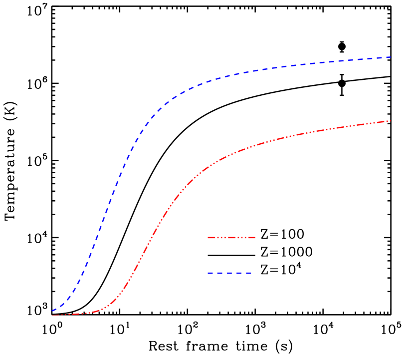
Figure 5: Temperature of the absorbing material as a function of time at a distance $R=100$ pc from the progenitor star. The left panel shows the results for the wind geometry while the right panel shows the shell geometry. Data are from the high resolution spectra of Fiore et al. (2005) as modeled in Fig. 2.

We use the time-dependent photoionization and dust-destruction code by Perna & Lazzati (2002; see also Perna, Lazzati & Fiore 2003) to follow the evolution of the dust distribution and of the ionization state of the gas under the intense flux of burst and early afterglow photons.

The column densities of CIV and SiIV provided by the simulations were converted into EW by using the full Voigt profile:

$$W_{\lambda}=\frac{\lambda^{2}}{c}\int^{\infty}_{0}1-e^{\frac{-\sqrt{\pi}e^{2}}{m_{e}c\Delta\nu_{D}}NfH(a,u)}d\nu$$ (8)

where $\Delta\nu_{D}$ is the Doppler width and $H(a,u)$ is the Voigt function given by:

$$\Delta\nu_{D}=\frac{\nu_{0}}{c}\sqrt{\frac{2kT}{m}}$$ (9)

$$H(a,u)=\frac{a}{\pi}\int^{\infty}_{-\infty}\frac{e^{-y^{2}}dy}{a^{2}+(u-y)^{2}}$$ (10)

The Voigt function parameters are $a=\Gamma/(4\pi\Delta\,\nu_{D})$ and $u=(\nu-\nu_{0})/(\Delta\,\nu_{D})$ and $\Gamma$ is the transition rate, approximated as $\Gamma=\gamma$, where $\gamma$ is the spontaneous decay rate.

The two systems $A$ and $B$ that make the high velocity absorption components are assumed to lie at the same distance from the burst since the data are not accurate enough to perform an independent fit. The two systems are blended in most of the medium resolution spectra from the literature. Thanks to the high resolution spectrum of Fiore et al. (2005), we can measure the ratio of CIV and SiIV column densities at $t=50$ ks as well as the temperature of the two absorbers (see Fig. 2). We derive temperatures of $T\sim 3\times 10^{6}$ K and $T\sim 10^{6}$ K for the systems $A$ and $B$, respectively. We also assume the same ionization for the two systems and conclude that system $A$ contains three times more material than system $B$.

The data for the high-velocity lines (the total EW for the $A$ plus $B$ components) are given in Tab. 1. There are two additional model parameters that must be selected before fitting the absorber properties as described above: the initial temperature of the absorber and its metallicity. The only constraint on metallicity comes from the spectroscopic observations of Mirabal et al. (2003) who detect Ly$\alpha$ absorption with proper motion of $\sim 3000$ km s^-1. Assuming that HI and CIV are the dominant ionic species of hydrogen and carbon, respectively, a metallicity of $\sim 1000$ is derived. However, given the temperature measured above, it is unlikely that the line ratio is a fair proxy to the metallicity and this datum must be taken with caution. For this reason we explore metallicities between $100$ and $10^{4}$ solar, with particular emphasis on the 1000 solar case (solar metallicities taken from Anders & Grevesse 1989). In all cases the He to H ratio is held solar as well as the Fe and Ni to H ratios, since WR winds are not supposed to be enriched of heavy elements that are synthesized in SN explosions. As we will see, the absorber temperature will provide additional evidence for this value of the metallicity.

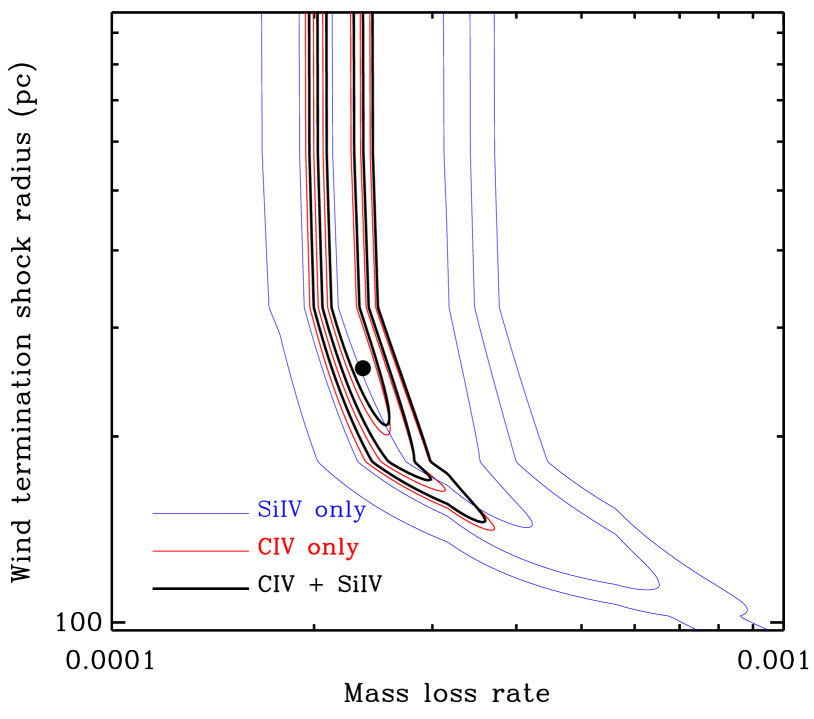
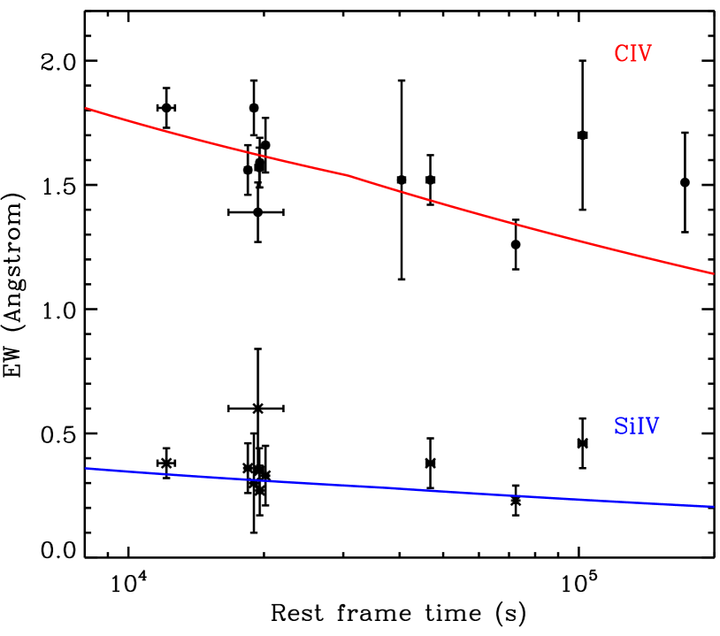
Figure 6: Best fit models for the wind geometry case. The left panel shows with a thick solid line the 1, 2 and 3 $\sigma$ confidence regions of the best fit model for the $Z=1000\,Z_{\odot}$ metallicity case. The broader contours (very thin blue line) show the confidence contours if only the SiIV data are considered. The medium thickness lines (red, almost indistinguishable from the thick ones) show the contours if only CIV is considered. The right panel shows the data with the best fit overlaid.

The initial temperature of the absorber could in principle be important since the ionic populations of CIV and SiIV vary sensibly around $T\sim 10^{5}$ K (Shull & Van Steenberg 1982). In local thermal equilibrium at $T=10^{6}$ K, only a minor fraction of CIV ($10^{-3.75}$) is expected and no significant presence of SiIV. This implies that the temperature of the absorbing blobs are affected by the burst irradiation. The irradiation temperature of the absorber depends on its metallicity, since the average ionization potential grows with metallicity. In Figure 5 we show the temperature of the absorber at the time of the high resolution spectroscopy of Fiore et al. (2005). In both the wind and shell case, high metallicity ($1000\,Z_{\odot}<Z<10^{4}\,Z_{\odot}$) produces temperatures in the observed range. A more accurate study cannot be performed since we fit a single zone model for the two absorbers while they have different temperatures. A different local metallicity or different radius can explain the difference.

Starling et al. (2005) considered a GRB jet characterized by a double structure, with a narrow component producing the GRB proper and a wider outflow producing the afterglow. They argued that in this case a lower mass loss rate and a smaller termination shock would agree with the data since most of the absorbing material would avoid the flash ionization caused by the prompt GRB phase. To check this idea we ran simulations with only the external shock afterglow component. We find that these simulations do not differ from our UV-poor model (the one widely explored in this work). Again, this is due to the fact that the optical-UV fluence is dominated in all cases by the external shock component. We therefore conclude that there is no evidence, from the spectroscopic data, that the jet of GRB 021004 had multiple components.

The results of our fits are reported in Table 3 for the wind case and in Table 2 for the shell (blob) case (see also Figures 6 and 7). Statistically, the two geometries are virtually indistinguishable. In both cases, the absorber lies at a distance of about 100 parsecs from the progenitor star (cf. also Fig. 8 for the wind case). This result is at odds with what previously discussed in the literature (Mirabal et al. 2003; Schaefer et al. 2003; Starling et al. 2005), where the flash ionization of the GRB and the early afterglow was not properly considered. It has important implications for the nature of the progenitor star and the ISM in which it is embedded.

It is important to note that this lower limit on the distance to the absorber is not due to the possible variability of the EWs. The fact that some CIV and SiIV absorption is seen several days after the GRB explosion requires the material to lie at a certain distance, otherwise all the CIV would be ionized to CV or higher and all the SiIV would be ionized to SiIV or higher. An order of magnitude estimate can be obtained by considering that the afterglow of GRB 021004 produced about $N_{\gamma}=4\times 10^{60}$ CIV ionizing photons. The ionization cross section of CIV is $\sigma_{CIV}=7\times 10^{-19}$ cm² (Verner & Yakovlev 1995). It follows that the distance of CIV ionization is approximately given, in optically thin conditions, by:

$$R=\sqrt{\frac{N_{\gamma}\,\sigma_{CIV}}{4\pi}}\sim 150\;\;{\rm pc}\;.$$ (11)

A more accurate estimate of the populations of CIV and SiIV can be seen in Fig. 8.

In addition to the reported fit, we performed test runs for the other continuum models described in $\S$ 3. As anticipated, we find that the change in the spectrum of the prompt emission affects the results only at a marginal level. We also investigated the difference between a dust rich (with solar dust-to-gas ratio and gas composition) and a dust poor environment (with all the elements in gaseous phase). Since the burst/afterglow are rich in UV radiation, the dust is thermally sublimated out to large radii. For this reason the results with and without an initial dust component are compatible within the errors, so we do not report them in detail here.

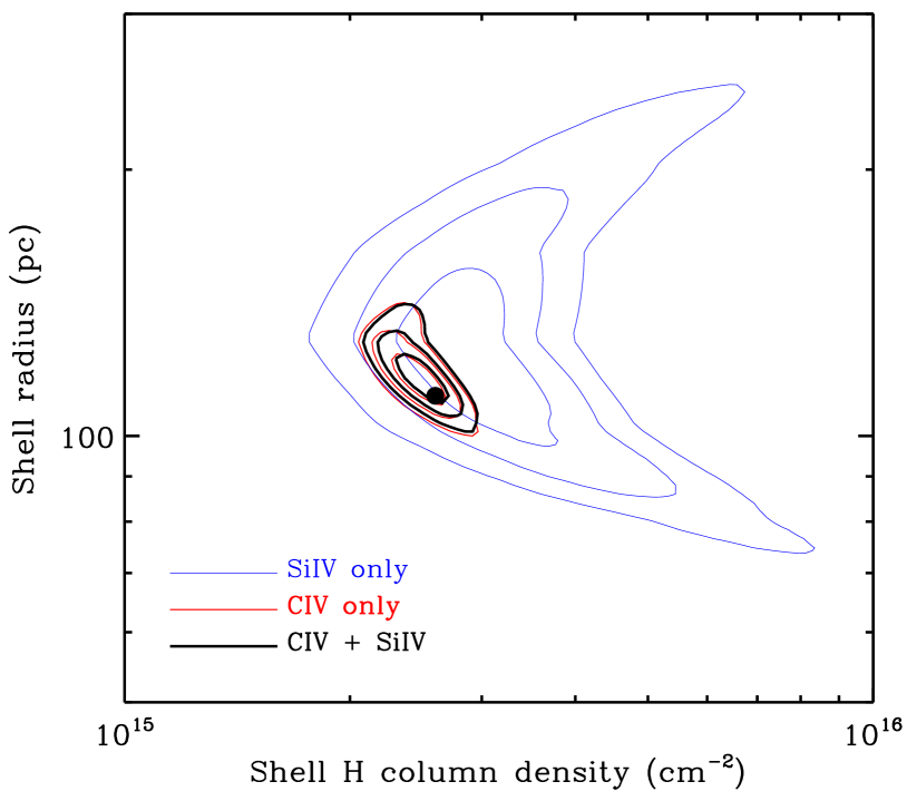
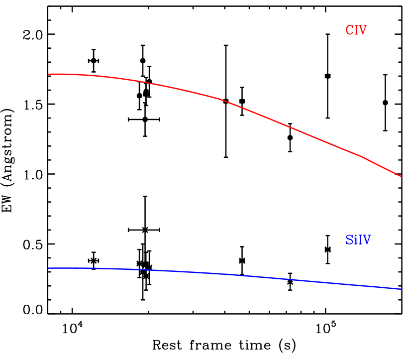
Figure 7: Same as Figure 6 but for the shell case.

For the wind case, the fit results are very similar, independent of the metallicity. In all cases the mass loss rate is relatively high, of the order of $10^{-4}$ solar masses per year. Given the distance from the burster and the wind speed, the episode of high mass loss took place approximately 30000 years before the GRB explosion.

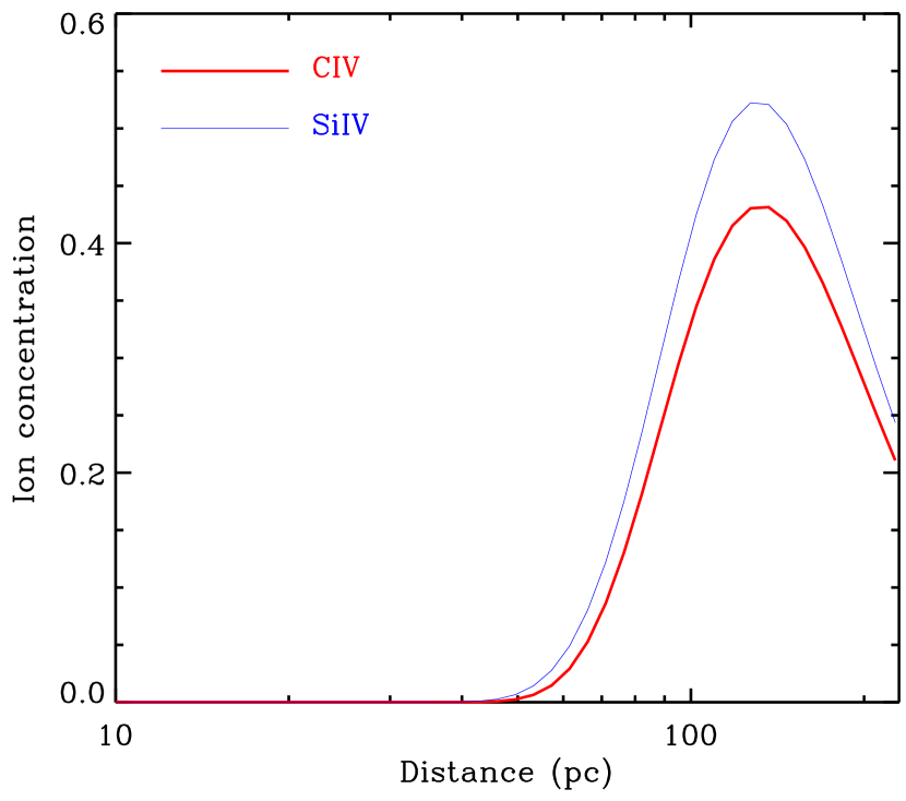
Figure 8: The radial distribution of the concentration of CIV (thick line) and SiIV (thin line) ions in the best fit wind model with metallicity 1000 solar (see text for more details. The concentrations are defined as the ratio of the ion density over the density of the element in any ionization status.

Table 1: Equivalent widths of the high-velocity lines. They are in Angstrom and in the GRB rest frame.

Time	error	element	lines	Wλ	error	ref.
40356.	1800	CIV	1548+1550	1.81	.08	(1)
40356.	1800	SiIV	1393.76	.38	.06	(1)
61202.7	900	CIV	1548+1550	1.56	.1	(3)
61202.7	900	SiIV	1393.76	.36	.1	(3)
63127.2	900	CIV	1548+1550	1.81	.11	(4)
63127.2	900	SiIV	1393.76	.3	.2	(4)
64422.	9000	CIV	1548+1550	1.39	.12	(5)
64422.	9000	SiIV	1393.76	.6	.24	(5)
64872.0	1300	CIV	1548+1550	1.57	.08	(6)
64872.0	1300	SiIV	1393.76	.35	.09	(6)
65044.1	900	CIV	1548+1550	1.59	.1	(7)
65044.1	900	SiIV	1393.76	.27	.1	(7)
66968.5	900	CIV	1548+1550	1.66	.11	(8)
66968.5	900	SiIV	1393.76	.33	.12	(8)
134275.	2400	CIV	1548+1550	1.52	.4	(2)
155592.	3000	CIV	1548+1550	1.52	.1	(6)
155592.	3000	SiIV	1393.76	.38	.1	(6)
240696.	900	CIV	1548+1550	1.26	.1	(6)
240696.	900	SiIV	1393.76	.23	.06	(6)
338832.	7000	CIV	1548+1550	1.7	.3	(9)
338832.	7000	SiIV	1393.76	.46	.1	(9)
571869.	3600	CIV	1548+1550	1.51	.2	(2)

References are: (1): Moeller et al. 2002; (2): Starling et al. (2005); (3): Our polarimetric spectra (0 rota); (4): Our polarimetric spectra (45 rota); (5): Schaefer et al. (2003); (6) Matheson et al. (2003); (7) Our polarimetric spectra (22 rota);(8) Our polarimetric spectra (67 rota); (9) Mirabal et al. (2003)

Table 2: Fit results for the wind geometry cases.

$T_{0}$ (K)	$Z/Z_{\odot}$	$R_{\rm{sh}}$ (pc)	$\dot{M}$ ($M_{\odot}$ y-1)	$\chi^{2}$ (prob)
$10^{3}$	$100$	$>215$	$(3.4\pm 0.4)\times 10^{-3}$	$22.9$ ($30\%$)
$10^{3}$	$1000$	$>210$	$(2.3\pm 0.3)\times 10^{-4}$	$22.9$ ($30\%$)
$10^{3}$	$10000$	$>80$	$(2.2\pm 0.3)\times 10^{-4}$	$22.9$ ($30\%$)

Table 3: Fit results for the shell geometry cases.

$T_{0}$ (K)	$Z/Z_{\odot}$	Radius (pc)	$N_{H}$ ($10^{15}$ cm-2)	$\chi^{2}$ (prob)	$M$ ($M_{\odot}$)
$10^{3}$	$1000$	$116_{-6}^{+14}$	$2.5\pm 0.3$	$28.3$ ($11\%$)	$86_{-3}^{+17}$
$10^{4}$	$1000$	$116_{-5}^{+14}$	$2.5\pm 0.3$	$28.3$ ($11\%$)	$86_{-4}^{+15}$
$10^{3}$	$100$	$121_{-9}^{+14}$	$28\pm 3$	$26.5$ ($15\%$)	$160_{-22}^{+44}$
$10^{3}$	$10000$	$121_{-9}^{+14}$	$0.28\pm 0.03$	$26.8$ ($14\%$)	$10_{-1.5}^{+2.5}$

5 Discussion

We have collected all the available spectroscopic data of GRB 021004 from the literature and compiled the time resolved evolution of the EW of CIV and SiIV absorption lines for the high velocity systems with $v\sim 3000$ km s^-1. We have then used our time dependent photoionization and dust-destruction code (Perna & Lazzati 2002) to model the evolution of the column densities of these ions under the intense radiation field of the GRB and its early afterglow. Previous work on subsets of these data (Mirabal et al. 2003; Schaefer et al. 2003; Starling et al. 2005) concluded that the observed absorption can be produced by material expelled by the GRB progenitor star under the form of a smooth wind. Wolf Rayet stars are the principal candidate due to the large speed and mass loss rate of their winds ((Nugis et al. 1998; Willis 1999 ; Nugis & Lamers 2000).

Wolf-Rayet stars are the final evolutionary stage of massive O-type stars, with initial main-sequence masses above about 35 M_⊙ (for solar metallicities). These stars eject material continuously in the form of line-driven winds. The observed mass loss rates of WC stars (those WR stars that show strong carbon lines) are $\sim 1-6\times 10^{-5}M_{\odot}{\rm yr}^{-1}$ and they produce winds with terminal velocities 800 - 3500 km s^-1 (Nugis et al. 1998; Willis 1999 ; Nugis & Lamers 2000). In the case of GRB progenitors there are not direct observations of the wind properties. Rykoff et al. (2004) argue that their mass loss may be substantially larger. Fitting the afterglow photometric data of GRB 030418 they find that a mass loss of $\sim 10^{-3}\,M_{\odot}$ yr^-1 is required.

WR wind terminal velocities can explain the observed blueshifted velocities we see within the high velocity system without invoking any further radiative acceleration mechanisms due to the GRB itself. In the conventional model of a wind-blown bubble formed by mass-loss from a massive star, the fast wind from a massive star expands into the slower ambient medium, which could be a fossil wind from a previous epoch, or even a molecular cloud. The fast wind sweeps up the medium into a thin, dense, swept-up shell. The high pressure behind this shell drives a reverse, or wind termination shock, into the freely expanding wind (Weaver et al. 1977; Dwarkadas 2005). Although WR stars form a late evolutionary stage of a massive star, which may undergo a large amount of mass-loss prior to the WR stage, this general picture provides a useful guide.

In this work we have shown how, by considering the flash ionization of the burst and early afterglow photons, we were able to further constrain the wind properties. In fact, the intense radiation flux fully photoionizes the gas and destroys dust particles out to a large radius. We have found that, in order for the remaining portion of the wind material at large radii to provide the required column density, the termination shock of the wind must lie at at least $\sim 100$ pc from the star and the mass loss rate from the progenitor star must have been large, of the order of $10^{-4}\,M_{\odot}$ per year. These constraints are much more restrictive than what concluded before and allow us to infer some important properties of the progenitor star. Once again, we emphasize how this conclusion does not depend on the possible decrease of the EW of the CIV line with time, but on the simple and robust observation of the presence of high velocity CIV several days after the burst explosion.

The value of the termination shock that we have determined is in the upper range of what generally discussed theoretically (Dwarkadas 2005; Fryer, Rockefeller & Young 2006). However, this large value can be achieved by a very massive progenitor evolving in a low-density environment. An illustrative example is shown in Figure 9, where we used a stellar evolution model provided by Meynet & Maeder (2003) for a 120 solar mass star. The model incorporates mass-loss from the star. We used the standard assumption that the velocity of the emitted wind is a given multiple of the escape velocity from the star at each time-step (Kudritzki & Puls 2000). The wind velocity and mass-loss rate are then used as input parameters to compute the evolution of the surrounding medium by means of the VH-1 code (Blondin & Lundqvist 1993; Dwarkadas 2005). As the star evolves, first as a main-sequence O star and then as a Wolf-Rayet star, the wind mass-loss parameters gradually change. The wind velocity, initially about 3500 km/s, drops to a low of about 1100 km/s and then increases again in the final stages to around 3000 km/s. The mass-loss rate increases from about $10^{-5}M_{\odot}$ yr^-1 to about twice that value. The ambient density was chosen to be about 10^-3 particles cm^-3, in order to have the wind termination shock form at a large radius (about 215 pc in this particular case). Our inference of a low-density environment for the progenitor of GRB 021004 could be interpreted within the context of the recent observations that some GRB progenitors have been expelled from their parent molecular clouds (Hammer et al. 2006). High velocity in OB stars are indeed not uncommon (Mdzinarishvili & Chargeishvili 2005). Another possibility for the creation of a low-density environment is that the massive star progenitor of the GRB was in a star cluster which created a superbubble; these structures are commonly observed in our own Galaxy as well as in nearby ones (e.g. Heiles 1978).

Figure 9: Characteristics of the bubble formed by the wind of a star of 120 $M_{\odot}$ expanding in a medium of density $10^{-3}$ cm^-3. The solid line shows the density (left y axis) while the dashed line shows the pressure (right y axis).

Finally, we have shown that a smooth wind is insufficient to fully account for the observations (Mirabal et al. 2003; Schaefer et al. 2003; Fiore et al. 2005; Starling et al. 2005). The structure in the velocity of the absorber suggests the presence of clumping, at least at a moderate level. To check if extreme clumping could explain the observations, we modeled the absorber as material concentrated in a shell of width $\Delta R=0.1R$, where $R$ is the radius of the shell. This configuration is relevant for the case of clumps with an angular size larger than the photon source (total covering). We found that the fits are statistically equivalent, but the physical constraints on the mass loss rate of the progenitor star are tighter ($\dot{M}\lower 2.15277pt\hbox{$\;\buildrel>\over{\sim}\;$}10^{-3}\,M_{\odot}$ per year). This is due to the fact that the material is more concentrated at a single radius with respect to a smooth wind.

The high resolution spectra of Fiore et al. (2005) allow us to set some constraints on the characteristics of the clumps. Since the line opacity is complete, the clumps must be larger than the source size. In addition, since we see two clumps, the surface filling factor must be close to unity. At the time of the observations, the transversal radius of the observable portion of the fireball is given by:

$$R_{\rm{fb}}(t)=c\,t\,\Gamma=3\times 10^{16}\frac{t}{2{\rm{days}}}\frac{\Gamma}{5}\qquad{\rm{cm}}$$ (12)

This is likely to be smaller than the dimension of clumps in the wind at a distance of $\sim 100$ parsec from the star.

It is possible that our estimate of the mass loss rate is moderately affected by the wind inhomogeneity. Consider a clumpy wind with a surface filling factor of $0.1$. In $90\%$ of the cases no high velocity absorption would be seen. Given that some absorption was detected, in $10\%$ of the cases velocity structure would be present. If this were the case, our $\dot{M}$ would be overestimated by a factor $\sim 10$.

These considerations on the presence of inhomogeneities in the wind of the GRB 021004 progenitor star should not come as a surprise. It has indeed been suggested for many years that WR winds are clumped (Moffat et al. 1988; Li et al. 2000). Clumping in the wind has been proposed as one scenario to solve the so-called “wind-momentum” problem present in these outflows. It has been noted by several authors that the momentum in the wind ${\dot{M}v_{\inf}}$ is several times the momentum flux (L/c) from the star (Barlow et al. 1981). Although this was initially explained away by scattering the radiation from the star more than once, it is unclear if there is sufficient opacity in the wind to accomplish this. Clumps solve this problem in two ways 1) by increasing the density and therefore increasing the luminosity by the $n^{2}$ factor in the emissivity (but see Brown et al. 2004) and 2) the consequence of clumping is to reduce empirically derived mass-loss rates of hot stars by about a factor of 3, thus reducing the wind momentum itself.

In summary, the complex spectra of GRB 021004 can be explained as a result of the absorption due to a very extended wind surrounding the GRB progenitor star. It also requires a sizably large mass loss rate of $\sim 10^{-4}\,M_{\odot}$ per year. The large radial development of the wind is likely due to a combination of the high mass loss, the wind speed and of a low density environment. Some degree of clumping is also required by the structure of the absorption in the velocity space. This study shows how time resolved medium-high resolution spectroscopy of the early GRB afterglow is a powerful tool to investigate the properties of the GRB environment and constrain the characteristics of the progenitor.

References

- [1] Anders, E., & Grevesse, N., 1989, Geochim. Cosmochim. Acta, 53, 197
- [2] Barlow, M. J., Smith, L. J., & Willis, A. J., 1981, MNRAS, 196, 101
- [3] Barraud C., et al., 2003, A&A, 400, 1021
- [4] Blondin, J. M., & Lundqvist, P. 1993, ApJ, 405, 337
- [5] Brown, J. C., Cassinelli, J. P., Li, Q., Kholtygin, A. F., Ignace, R., 2004, A&A, 426, 323
- [6] Draine, B. T. & Hao, L., 2002, ApJ, 569, 780
- [7] Dwarkadas, V. V. 2005, ApJ, 630, 892
- [8] Fiore, F. et al., 2005, ApJ, 624, 853
- [9] Fox, D. W., & Price, P. A. 2002, GRB Circular Network, 1671, 1
- [10] Fryer, C. L., Rockefeller, G., Young, P. A., 2006, ApJ 647, 1269
- [11] Hammer, F., Flores, H., D. Schaerer, D., Dessauges-Zavadsky, M., Le Floc’h, E., Puech, M., 2006, A&A 454, 103
- [12] Heiles, C. 1979, ApJ, 229, 533
- [13] Heyl, J. & Perna, R. 2003, ApJ, 586L, 13
- [14] Hjorth, J. at al., 2003, Nature, 423, 847
- [15] Holland S. T., Weidinger M., Fynbo J. P. U., et al., 2003, AJ, 125, 2291
- [16] Kudritzki, R-P. & Puls, J. 2000, ARA&A, 38, 613
- [17] Lamb D. et al. 2002, GCN 1600
- [18] Lazzati D., Rossi E., Covino S., Ghisellini G., Malesani D., 2002, A&A, 396, L5
- [19] Li, Q., Brown, J. C., Ignace, R., Cassinelli, J. P., Oskinova, L. M., 2000, ApJ, 357, 233
- [20] Li Z., Chevalier R. A., 2003, ApJ, 589, L69
- [21] Matheson, T. et al., 2003, ApJ, 582, L5
- [22] Mathis, J. S., Rumpl, W., & Nordsieck, K. H., 1977, ApJ, 217, 425
- [23] Mdzinarishvili T. G., Chargeishvili K. B., 2005, A&A, 431, L1
- [24] Meynet, G. & Maeder, A. 2003, A&A, 404, 975
- [25] Mirabal, N. et al., 2003, ApJ, 595, 935
- [26] Moeller, P. et al., 2002, A&A, 396, L21
- [27] Moffat, A. F. J., Drissen, L., Lamontagne, R., Robert, C., 1988, ApJ, 334, 1038
- [28] Nakar E., Piran T., Granot J., 2003, NewA, 8, 495
- [29] Nugis, T., Crowther, P. A., & Willis, A. J. 1998, A&A, 333, 956
- [30] Nugis, T., & Lamers, H. J. G. L. M. 2000, A&A, 360, 227
- [31] Perna, R. & Loeb, A. 1998, ApJ, 501, 467
- [32] Perna, R., & Lazzati, D. 2002, ApJ, 580, 261
- [33] Perna, R., Lazzati, D., & Fiore, F. 2003, ApJ, 585, 775
- [34] Rykoff, E. S. 2004, ApJ, 601, 1013
- [35] Sako, M., Kahn, S. M., Paerels, F., et al., to be published in “ High-resolution X-ray Spectroscopy Workshop with XMM-Newton and Chandra”, MSSL, Oct 24-25, 2002
- [36] Schaefer, B. et al., 2003, ApJ, 588, 387
- [37] Shull, J. M., Van Steenberg, M, 1982, ApJS, 48, 95
- [38] Stanek, K. Z. et al., 2003, ApJ, 591, L17
- [39] Starling, R. L. C. et al., 2005, MNARS, 360, 305
- [40] van Marle, A. J., Langer, N., García-Segura, G. 2005, A&A, 444,837
- [41] Verner, D. A., & Yakovlev, D. G., 1995, A&AS, 109, 125
- [42] Weaver, R., McCray, R., Castor, J., Shapiro, P., & Moore, R. 1977, ApJ, 218, 377
- [43] Willis, A. J. 1999, IAU Symp. 193: Wolf-Rayet Phenomena in Massive Stars and Starburst Galaxies, 193, 1