Bright Metal-Poor Stars from the Hamburg/ESO Survey.
I. Selection and Follow-up Observations from 329 Fields

Abstract

We present a sample of 1777 bright ($9<B<14$) metal-poor candidates selected from the Hamburg/ESO Survey (HES). Despite saturation effects present in the red portion of the HES objective-prism spectra, the data were recoverable and quantitative selection criteria could be applied to select the sample. Analyses of medium-resolution ($\sim 2$ Å) follow-up spectroscopy of the entire sample, obtained with several $2$ to $4$ m class telescopes, yielded 145 new metal-poor stars with metallicity $\mbox{[Fe/H]}<-2.0$, of which 79 have $\mbox{[Fe/H]}<-2.5$, and 17 have $\mbox{[Fe/H]}<-3.0$. We also obtained C/Fe estimates for all these stars. From this, we find a frequency of C-enhanced ($\mbox{[C/Fe]}>1.0$) metal-poor ($\mbox{[Fe/H]}<-2.0$) giants of $9\%\pm 2\%$, which is lower than previously reported. However, the frequency raises to similar ($>20\%$) and higher values with increasing distance from the Galactic plane. Although the numbers of stars at low metallicity are falling rapidly at the lowest metallicities, there is evidence that the fraction of carbon-enhanced metal-poor stars is increasing rapidly as a function of declining metallicity. For $\sim 60$ objects, high-resolution data have already been obtained; one of these, HE 1327$-$2326, is the new record holder for the most iron-deficient star known.

1. Introduction

The first systematic searches for metal-poor stars in the Galactic halo, by means of objective-prism surveys, began with Bond (1970, 1980, 1981) and Bidelman & MacConnell (1973). More recent surveys are the HK survey (Beers et al., 1985, 1992; Beers, 1999) and the Hamburg/ESO survey (HES; Wisotzki et al. 2000; Christlieb 2003). Over time, deeper surveys have became possible to reach further into the Galactic halo. The limiting magnitude of the HES is $B\sim 17.5$ mag as opposed to the earlier HK survey ($B\sim 15.5$ mag).

Particularly the HK survey and HES have both shown that a variety of astrophysically interesting and unusual objects can be found in a large sample of metal-poor stars. Some of these exhibit large overabundances of heavy neutron-capture elements that are synthesized in the s-process (e.g., Aoki et al. 2001; Van Eck et al. 2001), or in the r-process (e.g., CS 22892$-$052, Sneden et al. 1996, or CS 31082-001 Cayrel et al. 2001). In the case of strong r-process enhancement, nucleo-chronometry becomes possible based on the abundance of e.g., Th and U. Bright metal-poor stars are particularly useful for this task since the weak uranium line at 3859 Å is only detectable in very high-quality spectra. The availability of U, together with Th, as the U/Th chronometer drastically reduces the theoretical uncertainties on the derived ages, as compared to the more easily detectable Th/Eu ratio (Wanajo et al., 2002). Hence, a lower limit for the age of the Universe can be derived independently of other measurements such as WMAP (Spergel et al., 2006). Many C-enhanced metal-poor objects (hereafter CEMP; $\mbox{[C/Fe]}>1.0$) were discovered as they occur with increased frequency amongst metal-poor objects (e.g., Rossi et al. 1999). One of those is the very iron-deficient giant HE 0107$-$5240 ($\mbox{[Fe/H]}=-5.2$) that was found in a sample of $\sim 2000$ HES metal-poor candidates (Christlieb et al., 2002). This star provided critical observational material to the theories of the formation of the first objects in the Universe.

For elemental abundance studies involving isotopes, such as ⁶Li in metal-poor turnoff stars, or very weak and/or blended lines, such as uranium in some strongly r-process enhanced objects, it is crucial to be able to obtain high-resolution ($R>40,000$) spectra with a very high signal-to-noise ratio. Bright metal-poor stars are thus ideal targets. With the increased light-collecting power of current 8-10 m telescopes it is possible to achieve a $S/N$ of $200$ or more for such objects within reasonable exposure times.

Apart from the faint stars, the HES also contains large numbers of bright ($B<14$) stars. However, those have previously not been investigated. The main technical reason is the partial saturatation of the photographic plates, resulting in partially satured spectra. Despite an increased interest to search for more fainter metal-poor stars in the extended survey volume of the HES, recovering those brighter stars is well worth the effort, because they offer a variety of advantages over fainter stars. In general, for bright stars, the availability of various data sources, such as the photometric survey 2MASS (Skrutskie et al., 2006), or astrometric catalogs, e.g., US Naval Observatory CCD Astrograph Catalog (UCAC2; Zacharias et al. 2000), or the Southern Proper Motion Catalog (SPM3.1; Girard et al. 2004), provide useful additional information for the analysis of large samples of objects. Hence, more detailed analyses, including kinematic studies that make use of the full space motions, of many bright stars can be carried out more quickly and easily.

The HES thus provides the opportunity to quickly identify large numbers of bright metal-poor stars in a systematic fashion. Such objects provide important information in the intermediate magnitude range between the early objective prism surveys and the HES. For example, a second star, HE 1327$-$2326, with an extremely low iron abundance of $\mbox{[Fe/H]}=-5.4$ (Frebel et al., 2005, 2006; Aoki et al., 2006) was already recently discovered in the sample of bright HES stars discussed in this paper.

Here we present the sample of bright metal-poor candidates selected from the HES. The candidate selection is described in § 2, while the results of the follow-up observations of the sample are presented in § 3. In § 4 we outline our data analysis and the abundance results of the metal-poor stars found in the sample. In § 5 we briefly conclude with an outlook for future work concerning the newly-discovered stars.

2. The Hamburg/ESO Survey

2.1. Recovering the bright metal-poor stars

The HES is an objective-prism survey initially designed to search for bright quasars ($14<B<18$) in the southern sky (Wisotzki et al., 2000). Exploitation of the stellar content amongst the $\sim 4$  million digital spectra was initiated later. Thus far, 329 (out of 380) HES plates have been searched for metal-poor stars and other stellar objects, e.g., field horizontal branch stars (Christlieb et al., 2005) or DA white dwarfs (Christlieb et al., 2001b). The remaining plates have recently been processed and follow-up work is now underway.

The extraction and selection of objects in the HES from the photographic survey plates is described in the following. After the construction of an input source catalog using the Digitized Sky Survey (DSS), an astrometric transformation was established between the direct (photographic) and spectral plates that yielded the position of each object on the spectral plate. Thus, wavelength zero points were derived. The wavelength range of all HES spectra is set by the atmospheric cut-off at $3200$ Å and the sharp sensitivity cut-off of the IIIa-J emulsion at $5400$ Å. The survey spectra in the HES database were first classified into three groups: stars, ext, bright, with stars standing for spectra of point sources, ext for spectra of extended objects, and bright for possibly saturated spectra of point sources. These classes of spectra were extracted with different algorithms (Wisotzki et al., 2000). In particular, the spectra of objects above a saturation threshold were extracted by summing the values of the photographic density perpendicular to the dispersion direction in a wide range, and hence incorporating unsaturated regions of the cross-dispersion profile. This results in an extension of the dynamic range of the objective-prism plates by 2-3 magnitudes. Each object was assigned a 12 character HES designation such as “HE 1234$-$5678”. The digit combination is based on the B1950 coordinates of the object.

This paper investigates the stellar HES spectra classified as bright only. The main difference between star and bright is a brightness cut-off defined by the level of saturation. Figure 1 shows three bright survey spectra to demonstrate the different levels of saturation.

2.2. The calibration

We seek to select metal-poor stars in a wide color range, i.e., stars near the main-sequence turnoff point as well as subgiants and giants. Thus, it is important to apply a selection that takes into account the strength of the Ca II K line (which is the strongest metal absorption line in the optical wavelength range) as a function not only of the metallicity of a star, but also of its effective temperature. The strength of the Ca II K line can be measured in the HES spectra by means of the line index KP (a pseudo-equivalent width measurement in Å) as defined by Beers et al. (1999).

The algorithm we employ here to select such metal-poor candidates had previously only been used in conjunction with unsaturated spectra of faint stars (i.e., stars). Hence, it was first necessary to test whether or not the selection algorithm would be applicable to partially saturated spectra. We verified with HK survey stars (Beers et al., 1992) present on HES plates that the HES KP measurements are in good agreement with the measurements made in moderate-resolution (i.e., $\Delta\lambda\sim 2$ Å) follow-up spectra. However, the 298 HK survey stars used for this verification cover the magnitude range $13<B<14.5$, which corresponds only to the faint end of the bright sample (see Figure Bright Metal-Poor Stars from the Hamburg/ESO Survey. I. Selection and Follow-up Observations from 329 Fields for the $B$ distributions of the two samples). Later, we learned that for the brighter stars the saturation of their spectra becomes stronger, and results in a systematic underestimate of the KP index. Unfortunately, the same problem occurs for any stars with $\texttt{KP}>5$ Å, where the survey data underestimates the index strength, regardless the brightness of the star. It follows that the selection efficiency of metal-poor giants is low, because more metal-rich giants were mistaken as metal-poor. However, no metal-poor stars should be lost due this problem. This is illustrated in Figure Bright Metal-Poor Stars from the Hamburg/ESO Survey. I. Selection and Follow-up Observations from 329 Fields, where the KP measurements from the prism-survey are compared with those obtained from medium-resolution spectroscopic data.

It is also possible to measure the $B-V$ color directly from the HES spectra, using the “half power point” technique described by Wisotzki et al. (2000). The $B-V$ color of the unsaturated HES objects has an uncertainty of 0.1 mag (Christlieb et al., 2001a). Figure Bright Metal-Poor Stars from the Hamburg/ESO Survey. I. Selection and Follow-up Observations from 329 Fields shows that equally good results can be achieved for the HES bright stars fainter than $B\sim 13$. However, for the brighter stars the scatter increases significantly, and the $B-V$ color of the redder objects is systematically underestimated. This can be explained by the fact that the photographic emulsion is more sensitive in the red part of the HES spectra than it is in the blue. Thus, the saturation effects should appear first in the red, and they should be more pronounced for red stars. The consequences of this issue for our sample are further described in § 3.3.

2.3. The selection

In this section we briefly describe the selection of metal-poor candidates amongst bright HES stars. Initially, no CCD photometry was available for HES stars brighter than $B\sim 13$. Based on the results from the comparison with the HK survey sample, we concluded that the overall level of saturation was not too strong, and that the quality of our survey spectra would be sufficient to begin the search for bright metal-poor stars.

In the first step, we restricted the range of objects to be considered to $0.3<B-V<1.2$. This corresponds to stars redder than the main-sequence turnoff point for metal-poor stars of an age of about 12 Gyr, and bluer than the stars at the tip of the red giant branch. On both sides of the color range, the chosen cut-off allows for an error margin of about 0.1 mag. During the selection, we ignored any potential reddening of the stars. The HES stars are located at high galactic latitudes, and any reddening usually is considerably smaller than 0.1 mag (see e.g., Christlieb et al. 2005).

For the second step of the selection, we determined a cut-off line in the KP index versus $B-V$ color parameter space in the following way. A set of simulated stars with KP and $B-V$, equally distributed in the range 0–15 Å and 0.3–1.2 mag, was created. For these simulated stars, we estimated [Fe/H] using the techniques of Beers et al. (1999). All stars with metallicities in the range of $-2.6<\mbox{[Fe/H]}<-2.4$ were selected. A cut-off line was fit to this set of data. The result will be discussed in further detail in a forthcoming paper (N. Christlieb et al. 2006, in preparation). All HES stars with a KP index lower than the cut-off value determined for its $B-V$ color were selected as metal-poor candidates. This results in a metallicity cut-off at $\mbox{[Fe/H]}=-2.5$. Applying this technique yielded $5081$ raw candidates.

In the final step of the selection, the raw and extracted HES spectra of these objects and the corresponding area of the direct plates available in the DSS were inspected in order to eliminate false positives due to plate artifacts, scratches, dust on the HES plates, emulsion flaws, ghosts and object extraction at a slightly wrong position on the spectral plate (a mis-positioned extraction results in systematically too low values of the Ca II K index).

2.4. The visual inspection

The apparent strength of the Ca II K line at 3933 Å was visually estimated against the continuum. Depending on how strong the line appeared, the objects were classified into several metal-poor classes (mpc) : mpca — the spectrum clearly shows no Ca II K line; unid — it is unclear if a Ca II K line is visible in the spectrum or not; mpcb — a weak Ca II K line is visible; and mpcc — a significant Ca II K line appears against the continuum. The remaining stars were grouped into star — ordinary (metal-rich) star; hbab — hot horizontal branch A or B stars displaying (very) strong Balmer lines; art — plate artefact; ovl — overlap of spectra of optically close stars due to unfortunate dispersion direction; and gal — galaxy, the object appeared to be extended on the direct image of the DSS. We identified 3309 spectra as belonging to the non metal-poor classes.

This leaves 1767 bright metal-poor candidates to form our working sample. Figure Bright Metal-Poor Stars from the Hamburg/ESO Survey. I. Selection and Follow-up Observations from 329 Fields shows some examples of the four metal-poor classes, together with their follow-up spectra (see § 3 for more details). The division of the candidates into the classes resulting from the visual inspection is presented in Table 1.

For 1626 of the total 1767 stars there are HES $B$ magnitudes available; the remaining stars are beyond the bright end of the magnitude range covered by the photometric sequences used to calibrate the HES photometry (see Wisotzki et al. 2000 for a description of the HES photometry). The average magnitude of the bright stars is $B\sim 11.5$ mag. The B magnitude distribution of the sample of bright stars is shown in the top panel of Figure Bright Metal-Poor Stars from the Hamburg/ESO Survey. I. Selection and Follow-up Observations from 329 Fields, together with the distributions of the HK survey and the faint HES stars. All three samples complement each other in brightness, covering a range of almost 10 magnitudes.

Concerning the HES, one might expect that the sample of bright HES stars would smoothly add objects to the bright tail of the distribution of the faint HES stars. However, this is not the case. Rather, the combined HES stars show a bimodal distribution. The form of the distribution can be explained by a selection bias present in the sample of bright metal-poor candidates from the HES. As discussed in § 2.3 above, the saturation of the HES spectra of bright stars results in a systematic underestimation of their Ca II K line index, hence a large number of false positives enter the candidate sample. This effect is strongest for the brightest stars, thus, bright stars are strongly over-represented in the sample of bright metal-poor candidates.

If this explanation is correct, than the bimodal distribution should not be seen in the sample of confirmed HES metal-poor stars. Indeed, as shown in Figure Bright Metal-Poor Stars from the Hamburg/ESO Survey. I. Selection and Follow-up Observations from 329 Fields (thick lined envelope of bottom panel), the magnitude distribution is smooth when the false positives are removed.

2.5. Cross-correlation with other catalogs

In order to identify re-discovered stars in our sample and to gain additional information for as many sample stars are possible, a cross-correlation of the HES database with several catalogs was carried out. We identified stars in the 2MASS All Sky Data Release (Skrutskie et al., 2006) and obtained $J$, $H$ and $K$ magnitudes, in the UCAC2 (Zacharias et al., 2000) and in the SPM3.1 (Girard et al., 2004) catalog to retrieve proper motions. We then cross-correlated with the HK survey database, and found a number of stars from the HK survey in our sample. We also made use of the following catalogs: the non-kinematically selected stellar sample from Bidelman & MacConnell (1973), the kinematically selected metal-poor stars samples of Ryan & Norris (1991), and Carney et al. (1994). Finally, we made extensive use of the SIMBAD database. During this search many of our stars appeared in well-known surveys, such as the Guide Star Catalog, the Positions and Proper Motion Catalog, or the HIPPARCOS/TYCHO catalog. See Table 2 for the numbers of stars found in the catalogs and the SIMBAD database.

We are aware of $29$ stars in our sample known to have $\mbox{[Fe/H]}\lesssim-2.0$. It should be noted though, that, due to our selection criteria, our sample is supposed to only contain objects with $\mbox{[Fe/H]}<-2.5$. Hence, it is expected that stars with $\mbox{[Fe/H]}>-2.5$ are missing from our compilation of rediscovered objects. Many of these objects were found in several catalogs or studies. Twenty four of those are metal-poor stars. For $16$ of them, an analysis based on high-resolution spectroscopy can be found in the literature. The re-discovered HES stars are listed in Table 3, together with selected other names, as well as, where available, iron abundances based on medium- and/or high-resolution studies. For comparison, in column (2) we also list our final iron abundance estimate. Amongst the re-discovered stars are G64-12 (HE 1337+0012; Carney & Peterson 1981) and the well-known strongly r-process enhanced metal-poor star CS 22892-052 (HE 2214$-$1654; Sneden et al. 1996). These re-discoveries show that our technique is successful in finding metal-poor stars. We flagged the re-discovered stars as such and kept them in our database as reference objects and for statistical purposes (see § 4.2).

In Table 4 we list five rediscovered stars for which we determined $\mbox{[Fe/H]}<-2.0$, but which are horizontal-branch stars. From these rediscoveries, we learn that our technique also works for other types of stars (as long as the indices and colors are within their acceptable ranges): HE 0411$-$3558, for example, is a horizontal-branch (HB) star discovered by Beers et al. (1992) (CS 22186-005). They measured $\mbox{[Fe/H]}=-2.66$ from a medium-resolution spectrum, while Ryan et al. (1996) obtained $\mbox{[Fe/H]}=-2.77$ from high-resolution data. Our final estimate is $\mbox{[Fe/H]}=-2.86$, which agrees well with the two other iron abundances.

Our follow-up spectra do not include any gravity-sensitive indicators available which is accurate enough for allowing the determination of evolutionary status of the stars. Hence, our sample of metal-poor stars is likely to have some contamination by HB stars. The rediscovery of a HB star and a red HB star in our sample (as listed in Table 4) for which we measured $\mbox{[Fe/H]}<-2.0$ confirms this. To quantify the expected level of contamination in our sample, we determined the fraction of HB stars to metal-poor star in the catalog of Beers et al. (1992). Based on gravity-sensitive photometry, they classified all their spectra according to evolutionary status. It appears that amongst the more metal-poor stars in their sample, the frequency of HB stars is $5\%-10\%$. They also find $\sim 2\%$ RR Lyr variables. We thus conclude that the contamination by HB stars is acceptably low for our work, and does not pose any concerns to our conclusions.

Trying to identify the known metal-poor stars in our sample also suggested searching for stars that may have been lost in the process of visual inspection of the raw candidates. We checked all stars discarded during the inspection in the SIMBAD database. Of the 3309 stars, $\sim 1100$ had some sort of entry, and $\sim$250 of these had at least one reference listed. Only 5 stars have $\mbox{[Fe/H]}<-2.5$. Table 5 gives further details, including our classification of these stars. The two hbab classifications are not in disagreement with the original classification found in the literature (i.e., they are a hot turnoff star and horizintal branch star). Also, the object classified as ovl could technically not have been picked up as metal-poor.

From a cross correlation with the HK survey database, we identified 44 stars, of which 30 are known to be A-type stars (Wilhelm et al., 1999; Beers et al., 1996b). Of those 30, we classified 27 as hbab, while the remainder are ovl. The 4 emission-line objects and the one RR Lyr star were all correctly classified as star, and hbab, respectively. The remaining HK stars are more metal-rich than $\mbox{[Fe/H]}=-2.5$.

We conclude that no stars were missed that should have been selected by our algorithm. Based on this result, we infer that our visual selection mechanism works very well to select the most metal-poor stars in a given sample of pre-selected HES candidates.

3. Medium-resolution follow-up spectroscopy

3.1. Observations

The HES objective-prism spectra have a resolution of $\sim 10$ Å (i.e., $R=\lambda/\Delta\lambda\sim 400$) at the Ca II K line, and an average S/N ratio of $\sim 8/1$, which is of sufficient quality to select metal-poor candidates in large numbers. To obtain a more reliable estimate of the metallicity than was known from the survey data, higher-quality spectra were needed. Hence, medium-resolution follow-up observations were taken with several telescopes (SSO $2.3\,$m, KPNO $4\,$m, CTIO $1.5\,$m, ESO $3.6\,$m, CTIO $4\,$m, AAT $3.9$ m) in the periods Mar – Apr 2003, Aug 2003 – Apr 2004, and Sep – Oct 2004. The spectra were obtained with a wavelength range covering at least $3600-4800$ Å, with $R\sim 2,000$ and $S/N>20/1$ at the Ca II K line. Exposure times during good weather conditions varied between $t_{\rm{exp}}\sim 20-300$ s. Using longer exposure times, these stars could also be observed through thin clouds or during periods with poor seeing (i.e., FWHM $>2\farcs 0$). See Table 6 for more details on the follow-up observations. Due to the low spatial resolution of the DSS, from which the HES input catalog was created, several spectra of two stars with small angular separation (i.e., $\lesssim 3\farcs 0$) were not spatially resolved on the survey plates. Hence, the “pair” was recorded with only one HES designation. We identified $10$ of these “pairs” in the course of the medium-resolution observations. Since it was not possible to decide which of the two stars would have been the correct metal-poor candidate, both were observed, and the sample size consequently increased to 1777 objects.

3.2. Data reduction and processing

Depending on where the data were obtained, the reduction of the spectra was carried out using different software. SSO data were fully reduced with Figaro (Shortridge, 1993) and Fortran programs, the KPNO and CTIO data with IRAF routines, the ESO data with ESO/MIDAS (Warmels, 1992), and the AAT data with IRAF.

Radial velocities of the targets were determined, and the spectra shifted to the restframe. To obtain the most accurate radial velocities as possible from medium-resolution spectra we used the combined results of two different methods: (1) Measuring the position of the Balmer lines H$\beta$, H$\gamma$ and H$\delta$ and (2) Fourier cross-correlation template matching with a grid of model atmosphere synthetic spectra with different temperatures, gravities and metallicities.

From comparing the results obtained with the two methods, we found a systematic offset of $\sim 10$ km s^-1 of the cross-correlation method with respect to the Balmer line results. However, we verified with observations of several standard stars taken during the program that the Balmer line method had no offset. To correct this effect, we removed the offset from the cross-correlation radial velocities. We adopted a weighted average of the two radial velocity measurements, where available. The velocity uncertainties of the two methods are of the same order. The median of the weighted uncertainty in the Balmer line method is $\sim 7$ km s^-1 whereas it is $\sim 4$ km s^-1 in the cross-correlation method. The advantage of the cross-correlation method is that information from the entire spectrum is used rather than just three individual lines as in the Balmer line method. This leads to a more precise velocity determination with a lower uncertainty. The median of final, weighted velocity uncertainty is $\sim 3$ km s^-1. Further systematic uncertainties, e.g., due to telescope/instrument instabilities, have not been considered.

We seek to use [Fe/H] as a metallicity indicator of the stars. However, iron lines are not detectable in our medium-resolution spectra, particularly in those of our targeted metal-weak stars. Instead, the Ca II K resonance line at $3933$ Å is very strong and can easily be measured. We employ the Ca II K calibration of Beers et al. (1999) to estimate [Fe/H] for each program star. This is done using the Ca II K line index KP (Beers et al., 1999) and $B-V$. The KP index is obtained by comparing the mean flux of two continuum regions around the Ca II K line with the flux of the Ca II K line itself. Regarding the color, we use two differently derived estimates. (1) The color $(B-V)_{\rm J-K}$ obtained from the dereddened 2MASS $J-K$ (see § 3.3), and (2) the spectroscopically derived $(B-V)_{\rm HP2}$ color based on the HP2 line index and the Beers et al. (1999) method. The HP2 index is a measurement of the strength of the H$\delta$ line, which depends on the effective temperature of the star, and hence its color. An advantage of using a color derived from the HP2 index is its independence of reddening. Finally, we measure the Beers et al. GP index from a comparison of the mean flux of two continuum regions with the flux of the CH band (G-band) at 4300 Å. We use the GP index to calculate carbon abundance estimates of all stars with $\mbox{[Fe/H]}<-1.0$ (see § 4.3).

3.3. Comparison with accurate photometry

CCD photometry was obtained for 84 stars in the sample. Additional photoelectric photometry (e.g., Beers et al. 1985, 1992; Norris et al. 1999; Anthony-Twarog et al. 2000) is available for 298 HK survey stars rediscovered in the HES (see also § 2.2). We compared these data with the HES $B$ magnitudes initially derived from the DSS direct plates. The agreement is good, as shown in Figure Bright Metal-Poor Stars from the Hamburg/ESO Survey. I. Selection and Follow-up Observations from 329 Fields. The saturation effects present in the spectra, however, were expected to have an influence on our $B-V$. We used the combined data to test this. Figure Bright Metal-Poor Stars from the Hamburg/ESO Survey. I. Selection and Follow-up Observations from 329 Fields presents the comparison of the $B-V$ colors. There is a clear deviation from the one-to-one $B-V$ relationship with the brightness of the objects. From a division of the stars into three brightness bins it is apparent that the saturation effects set in for stars brighter than $B=13$, thus spoiling the survey color measurements for these stars. In retrospect, this somewhat contradicts our previous finding that the survey color measurements would not be strongly influenced by saturation effects (see § 2.2). However, this discrepancy can be understood for the following reason. Previously, we used a sample that was too faint to be consistent with our average brightness of $B\sim 11.5$ mag.

We had no knowledge at the outset of our project that the onset of the saturation occured at $B\sim 13$, which is the brighter limit of the HK survey calibration sample. As a consequence, we decided not to use the survey colors but replace them with new $B-V$ derived from the 2MASS $J-K$ colors. We obtained a regression for a sample of stars with known $B-V$ and $J-K$ colors (i.e., $B-V=0.2+0.642(J-K)+0.707(J-K)^{2}$). For the cases where no $J-K$ color was available we used colors derived from the HP2 index, failing which we adopted the original survey color. The new $B-V$ colors agree well with those derived from the HP2 index for stars with $B-V<0.7$. As expected, for stars cooler than this, the index becomes insensitive to temperature and the quality of the colors degrades.

The $(B-V)_{J-K}$ color distribution is shown in Figure Bright Metal-Poor Stars from the Hamburg/ESO Survey. I. Selection and Follow-up Observations from 329 Fields (hatched distribution). The majority of stars are turnoff stars ($B-V\sim 0.4$), with several stars hotter than $B-V=0.3$, which was our initial blue limit for the selection of the sample. From the clear distribution of initial HES colors in Figure Bright Metal-Poor Stars from the Hamburg/ESO Survey. I. Selection and Follow-up Observations from 329 Fields, it is apparent that the new, $(B-V)_{J-K}$, colors are bluer than $(B-V)_{\rm{HES}}$, and in agreement with the results from the photometric colors. This effect could explain why many A-type stars, rather than metal-poor stars, were found in the sample (for further discussion, see § 4.7).

Concerning the selection algorithm, we conclude that it will function correctly only if the survey $B-V$ color is replaced with a better estimate, such as one based on the 2MASS data.

4. Analysis of the sample

4.1. Iron abundance estimates

As described in § 3.2, we use the Ca II K line to estimate the iron abundance for each star. However, we first excluded all stars from the sample that were obviously misclassified, e.g., objects with He lines or Ca II K emission-line cores in the medium-resolution spectra. After that, we attempted to obtain abundances for stars with a KP index, in the range $0.0<\texttt{KP}\leq 9.5$ in three ways:

1. $\mbox{[Fe/H]}_{\rm{B-V}}$: Employing the Beers et al. (1999) calibration using the KP index together with the color derived from the dereddened 2MASS $J-K$ data, $(B-V)_{\rm J-K}$. For this method to be applicable, the color has to lie in the range $0.3<(B-V)_{\rm{J-K}}<1.0$.

2. $\mbox{[Fe/H]}_{\rm{HP2}}$: Employing the Beers et al. calibration using the KP index, together with the color derived from the HP2, $(B-V)_{\rm HP2}$. The index has to lie in the range $0.25\leq\texttt{HP2}\leq 5.3$

3. $\mbox{[Fe/H]}_{\rm{Rossi}}$: Iron abundance estimates using the regression provided by Rossi et al. (2005), based on the KP index and the 2MASS $J-K$ color. For the $J-K$ de-reddening, we adopted the approach of Bonifacio et al. (2000) to infer $E(J-K)$ from the Schlegel et al. (1998) $E(B-V)$. Following Rossi et al., the color has to lie in the range $0.2\leq(J-K)_{0}\leq 0.8$.

The ranges of the indices and colors are imposed by the limits of the calibrations used. Depending on the above criteria, not all methods could always be employed for each star, and many have only a partial set of iron abundance estimates.

We note that this work focuses on the identification of the more metal-poor stars in the sample. We thus concentrate on all objects with $\mbox{[Fe/H]}<-1.0$, and do not give further consideration to stars with higher metallicities. $\mbox{[Fe/H]}=-1.0$ is the upper metallicity limit of all the calibrations employed in this work, because the KP index begins to saturate for stars more metal-rich than $\mbox{[Fe/H]}\sim-1.5$ (Beers et al., 1999). We did not attempt to make use of the auto-correlation function technique (ACF; Beers et al. 1999) to determine iron abundance estimates for the stars more metal-rich than $\mbox{[Fe/H]}\sim-1.5$ in our sample. This would be beyond the scope of the present investigation of finding the more metal-poor stars in this sample. However, for a full kinematic analysis it would be desirable to obtain better abundance estimates for such stars.

To best determine whether a star has $\mbox{[Fe/H]}>-1.0$ we applied the following procedure. We weighted and averaged the abundances $\mbox{[Fe/H]}_{\rm{B-V}}$ and $\mbox{[Fe/H]}_{\rm{HP2}}$ to form the best estimate based on the Beers et al. (1999) method, $\mbox{[Fe/H]}_{\rm{HP2/B-V}}$. Compared to the values determined from the Rossi et al. 2005 calibration, we regarded the former to be the more robust estimates. We then discarded the iron abundance estimate of all stars with $\mbox{[Fe/H]}_{\rm{HP2/B-V}}>-1.0$. On the other hand, when the star had $\mbox{[Fe/H]}_{\rm{HP2/B-V}}<-1.0$, we averaged the $\mbox{[Fe/H]}_{\rm{B-V}}$ and $\mbox{[Fe/H]}_{\rm{Rossi}}$ values to form a best estimate based on the $J-K$ colors, $\mbox{[Fe/H]}_{\rm{J-K}}$. The $\mbox{[Fe/H]}_{\rm{HP2/B-V}}$ was not further considered. Finally, we were left with one abundance derived from the HP2 index ($\mbox{[Fe/H]}_{\rm{HP2}}$), as well as one obtained from the $J-K$ ($\mbox{[Fe/H]}_{\rm{J-K}}$).

Before calculating the final iron abundance from the $\mbox{[Fe/H]}_{\rm{HP2}}$ and $\mbox{[Fe/H]}_{\rm{J-K}}$ for the remaining stars, we weighted the methods according to their temperature sensitivity. We tested the change of the iron abundances to small variations of the input HP2 indices and $J-K$ colors. From that, we estimated that for stars with $\texttt{HP2}>2.5$ the iron abundances derived from the HP2 indices are more robust than those based on the $J-K$ colors. For stars with $\texttt{HP2}\leq 2.5$, both methods appeared to be about equally good. $\texttt{HP2}=2.5$ corresponds to $B-V\sim 0.5$, which automatically results in a division of dwarfs ($\texttt{HP2}>2.5$) and giants ($\texttt{HP2}\leq 2.5$). We note that in a magnitude-limited survey like ours, stars at $B-V>0.5$ are almost exclusively giants. The survey volume for cool dwarfs is neglible compared to the survey volume for the higher luminosity giants, which are seen up to much larger distances. In the following, we refer to dwarfs and giants according to their HP2 index. This is also the lower, cooler, limit at which the HP2 index begins to lose sensitivity to the $B-V$ color. Additionally, we split the dwarfs and the giants each into carbon-abundance-sensitive GP-strong and GP-normal categories. When calculating the final average iron abundance of GP-strong stars, no values from $\mbox{[Fe/H]}_{\rm{HP2}}$ were used. The appearance of a strong G-band at $4300$ Å may spoil the HP2 measurement. We used $\texttt{GP}>5.0$ as a limit for giants and $\texttt{GP}>4.0$ for dwarfs. With decreasing iron abundance, it is increasingly likely that GP-strong stars are very carbon rich (see also discussion in § 4.3).

Depending on availability of the various [Fe/H] estimates, we weighted and averaged the values to obtain the final estimate $\mbox{[Fe/H]}_{final}$. Table 7 shows the weights (for dwarfs and giants seperately) for each of the two iron abundance estimates used to form a specific, averaged value. In total we have identified $16\%$ of the sample stars to be genuinely metal-poor (i.e., 286 objects with $\mbox{[Fe/H]}<-1.0$). Table 8 lists further details on how many stars were found below a given metallicity. We note that more than half of these stars are giants (189 out of 286), despite the fact that our sample of 1777 stars comprises mostly dwarfs.

Due to the lower effective temperature, metal-poor giants are better candidates than dwarfs amongst which to search for e.g., strong r-process enhancement. The cooler the temperature, the stronger the absorption lines appear. This is of importance when searching amongst metal-deficient stars where lines are expected to appear weak. The use of such giants then allows the tracing of r-process enhancement down to the lowest metallicities.

Taking the number of previously identified metal-poor stars into account, the numbers of newly-discovered metal-poor objects in this work are shown in Table 8. For completeness, we also list the number of literature stars for which a high-resolution analysis has been reported.

We note here that for the most iron-poor star HE 1327$-$2326, a metallicity of $\mbox{[Fe/H]}_{final}=-4.3$ was obtained, based on its medium-resolution spectrum. The extremly low metallicity of [Fe/H]$=-5.4$ was only determined from high-resolution spectra. The discrepancy is due to interstellar Ca blending with the Ca II K line, which could not be resolved in the medium-resolution data. The overall metallicity covered by our sample ranges from $\mbox{[Fe/H]}_{final}=-4.3$ up to $\mbox{[Fe/H]}_{final}=-1$ (chosen upper limit).

4.2. Effective yields and the metallicity distribution function

In the present context, the “effective yield” describes the fraction of genuine metal-poor stars below a certain metallicity, compared with the total number of targeted stars (Beers, 2000). In Table 9 we compare the “effective yields” of our bright metal-poor stars with the faint HES and HK survey stars (data taken from Beers & Christlieb 2005). We obtain significantly lower overall effective yields for our work in comparison with the HES faint sample. This is not unexpected. Saturation effects had an important (negative) impact on the survey colors by which the bright metal-poor candidates were selected (see § 2.2), and led to the majority of the entire sample falling outside our criteria for potential metal-poor stars (see § 4.1). Apart from saturation issues, the majority of the sample is bright and thus likely to be relatively nearby. They might belong to the thick disk rather than the halo. Hence, the contamination by more metal-rich stars is larger compared to the sample of the HES faint stars, which is claimed to comprise $\sim 50\%$ stars with $\mbox{[Fe/H]}<-2.0$ (Beers & Christlieb, 2005). However, when comparing our effective yields with those of the HK survey (in its initial design with no available colors) they are of the same order.

The metallicity distribution function (MDF) of the stars with $\mbox{[Fe/H]}<-1.0$ from the HK survey and our bright star sample is presented in Figure Bright Metal-Poor Stars from the Hamburg/ESO Survey. I. Selection and Follow-up Observations from 329 Fields. Both samples include dwarfs and giants. The HES bright distribution for stars with $\mbox{[Fe/H]}<-1.0$ has one main peak at $\mbox{[Fe/H]}\sim-2.3$. This peak likely arises from the fact that the initial selection of bright stars was aiming to find stars whose Ca II K line strengths measured in the survey spectra indicated a metallicity of $\mbox{[Fe/H]}\lesssim-2.5$. Thus, in the case that the selection works well, the majority of the genuine metal-poor stars confirmed after the medium-resolution observations should spread around $\mbox{[Fe/H]}\sim-2.5$. This explanation is supported by the fact that almost half of the stars with $\mbox{[Fe/H]}<-1.5$ are fainter than $B=13$. Hence, this subsample does not contain as many of the brighter stars, whose initial selection as metal-poor candidates was influenced by saturation effects. However, the dip in the distribution at $\mbox{[Fe/H]}=-2.5$ cannot be explained in this way. No explanation, other than this may be a low number statistical effect, can currently be found for this dip.

Towards the higher metallicity cut-off of the MDF the number of stars rises significantly, likely due to incorrectly-selected objects. There is a link between a low selection efficiency and the brightness of the objects due to the saturation effects. About 95% of the stars in the range of $-1.5<\mbox{[Fe/H]}<-1.0$ are brighter than $B=13$. This is the brightness limit at which the saturation becomes much more severe for brighter stars. The combination of [Fe/H] uncertainties, e.g., from the limits of the calibrations itself or the loss of sensitivity to metallicity from $\mbox{[Fe/H]}\sim-1.5$ upwards, likely causes objects with a true $\mbox{[Fe/H]}>-1.0$ to appear in our MDF as metal-poor stars.

We wish to emphasize that despite the low overall effective yields, this sample has produced astrophysically important metal-poor stars. Based on our ongoing high-resolution observations of the most metal-poor stars from this sample we have found HE 1327$-$2326 ($\mbox{[Fe/H]}<-5.4$) and at least one strongly r-process enhanced star ($\mbox{[r/Fe]}\sim 2.0$, A. Frebel et al. 2006, in preparation). Results on further stars will be reported elsewhere (see also § 5).

4.3. Carbon abundance estimates

Metal-poor stars with enhanced carbon abundance are important to investigate, for example, the shape of the initial mass function and the formation and evolution of the first generations of stars. In recent years it has become apparent that the number of carbon-rich stars increases with decreasing metallicity (e.g., Beers & Christlieb 2005). The origin of this trend is not well understood. Our sample is well suited to investigate the frequency of CEMP stars amongst metal-poor stars.

One way to recognize carbon rich stars among metal-poor objects is by their G-band strengths (e.g., $\texttt{GP}\gtrsim 4.5$). Amongst the 1777 stars in our sample, $216$ have $\texttt{GP}>5$. Only $30$ stars, however, have $\texttt{GP}>6$, while $6$ objects have $\texttt{GP}>7$. When considering the subsample of stars with $\mbox{[Fe/H]}<-1.0$, the numbers become 43, 16, and 6, respectively. The index begins to saturate from $\texttt{GP}\sim 6$ but certainly, $\texttt{GP}\gtrsim 6$ indicates a very strong G-band. If the metallicity of a star is low and the GP index large, the star is very likely to be rich in C. Figure Bright Metal-Poor Stars from the Hamburg/ESO Survey. I. Selection and Follow-up Observations from 329 Fields illustrates a sequence of strengths of the G-band and the corresponding C abundance based on the Rossi et al. (2005) calibration (see below). As an example, we measured a G-band strength of $\texttt{GP}\sim 5.0$ for CS 22892$-$052, the well-studied r-process- and CEMP star which was rediscovered in our sample. Beers et al. (1992) obtained $\texttt{GP}\sim 5.5$ from their medium-resolution spectrum. They also derive $\mbox{[Fe/H]}=-3.0$, while we obtain $\mbox{[Fe/H]}=-3.1$. McWilliam et al. (1995) then obtained a carbon abundance of $\mbox{[C/Fe]}\sim 1.0$ (from high-resolution data), which is in good agreement with our value of $\mbox{[C/Fe]}=1.2$.

In general, the carbon abundance (with respect to H or Fe) can best be determined from high-resolution observations. In the absence of such data for the entire sample of stars with $\mbox{[Fe/H]}<-1.0$ we rely on a different approach. We use the newly available calibration of Rossi et al. (2005) to obtain estimates for the relative carbon abundances, [C/Fe]. Their regression is suitable for an analysis based on the KP and GP indices measured in medium-resolution spectra. We added the constraint $\texttt{GP}\geq 1.0$ to ensure that the G-band was clearly present in the spectrum. See Table 10 for the numbers of mildly ($\mbox{[C/Fe]}>0.5$) and strongly ($\mbox{[C/Fe]}>1.0$) carbon-enriched objects found amongst the 53 dwarfs and 121 giants with $\mbox{[Fe/H]}<-2.0$ in our study. The lower limits given in the table are due to the constraint on the GP index to be larger than 1.0, which introduces a bias against carbon-rich dwarfs. Figure Bright Metal-Poor Stars from the Hamburg/ESO Survey. I. Selection and Follow-up Observations from 329 Fields then shows [C/Fe] for the 234 objects with $\texttt{GP}>1.0$ and $\mbox{[Fe/H]}<-1.0$, plotted against their iron abundances [Fe/H]. An increased spread of carbon abundances with decreasing iron abundance is clearly seen. However, some stars are missing from the figure because we have not calculated C abundances for objects with low G-band strength (i.e., $\texttt{GP}<1.0$). Those stars would likely have low levels of C enhancement. As a consequence of this constraint on the GP index most of our metal-poor dwarfs have no carbon abundance estimate. Due to their higher temperature, the dwarfs are more strongly affected by this constraint than the giants. Hence, we note here that we did not attempt to derive a relative frequency of CEMP dwarfs. It is also worth mentioning that no [C/Fe] was estimated for the most iron poor dwarf/subgiant HE 1327$-$2326. There is no G-band visible in our medium-resolution spectrum ($\texttt{GP}=0.5$). Additionally, no stars similar to HE 1327$-$2326 are available in the calibration (Rossi et al., 2005). Any derived value for such a star would thus be untrustworthy. Finally, several authors in the literature have noted a general upper limit of C enhancement with respect to the Sun only (e.g., Ryan 2003, $\mbox{[C/H]}\sim-1.0$). We also find such an envelope at $\mbox{[C/H]}\sim-0.7$. However, we note that W. Aoki et al. (2006, in preparation) and S. Lucatello et al. (2006, in preparation) find an upper limit on carbon enhancement for carbon-enhanced metal-poor stars close to [C/H] = 0.0.

4.4. The frequency of C-enhanced metal-poor stars

If we now only consider the giants with $\mbox{[Fe/H]}<-2.0$ (which make up $\sim 70\%$ of the objects below that limit), we find the frequency of metal-poor giants with a strong carbon enhancement of $\mbox{[C/Fe]}\geq 1.0$ to be $\sim 9\%\pm 2\%$. If we take giants with $\mbox{[Fe/H]}<-2.5$, the frequency rises to $13\%\pm 4\%$, and to $25\%\pm 11\%$ amongst giants with $\mbox{[Fe/H]}<-3.0$. The uncertainties are based on Poisson statistics. One potential reason for the low percentage of carbon-enhanced stars below $\mbox{[Fe/H]}=-2.0$ may be that, for stars with $\texttt{GP}>6.0$, the calculated [C/Fe] has been underestimated by as much as 0.5 dex (Rossi et al., 2005). We have two stars with $\texttt{GP}=7.5$ and 7.9 which both have $\mbox{[C/Fe]}=0.9$. Thus, they fall just below our cut-off of 1.0. If those stars were to have an underestimated [C/Fe] by only 0.1 dex, the frequency of giants with $\mbox{[Fe/H]}<-2.0$ would rise to $11\%\pm 3\%$.

We note here that our frequency estimates are not affected by the constraint on the GP index (see above). Only stars with $\mbox{[C/Fe]}>1$ were counted and compared to the total number of stars with $\mbox{[Fe/H]}<-2.0$, $-2.5$ and $-3.0$, respectively. There clearly is a metallicity effect on the frequency of CEMP stars. It almost triples when stars with $\mbox{[Fe/H]}<-3.0$ are compared with those having $\mbox{[Fe/H]}<-2.0$. This is reflected in the larger spread of [C/Fe] with decreasing iron abundance.

Our average frequency of CEMP stars of $9\%$, however, is much lower than what is quoted in Beers & Christlieb (2005). They mention “at least 20%” amongst stars with $\mbox{[Fe/H]}<-2.0$. For a different sample of HK survey stars with $\mbox{[Fe/H]}<-2.5$, Marsteller et al. (2005) even find $\sim 25\%$ of the stars to be enhanced in carbon. Our low frequency is, in any case, of the same order as what was found by Cohen et al. (2005) ($14\%\pm 4\%$). S. Lucatello et al. (2006, in preparation), however, report that at least 20% of the stars with $\mbox{[Fe/H]}<-2.0$ from the large HERES sample of Barklem et al. (2005), based on high-resolution spectroscopic determinations, exhibit $\mbox{[C/Fe]}>1.0$.

We investigated the apparently low frequency farther by taking the sample of Beers, Preston & Shectman (1992; hereafter BPSII) to derive the percentage of their CEMP stars in the same fashion as adopted in the present work. A subsample of giants with $\texttt{HP2}<2.0$ was taken and [Fe/H] and [C/Fe] derived according to the Beers et al. (1999) method and the Rossi et al. (2005) calibration, respectively. The subset of objects with $\mbox{[Fe/H]}<-2.0$ and $\mbox{[C/Fe]}>1.0$ was then compared to our sample after applying the same constraints. Despite the different brightness and color distributions, as well as a different distance distribution (the BPSII sample being a little fainter and on average further away), we find their sample to have the same, low, percentage as obtained for ours ($\sim 9\%$). We note that by using the Beers et al. (1999) method to obtain the iron abundance estimates, we are also able to obtain estimates for the absolute magnitudes and distances of our stars.

We then tested whether there would be a variation in percentage with distance $Z$ from the Galactic Plane. Figure Bright Metal-Poor Stars from the Hamburg/ESO Survey. I. Selection and Follow-up Observations from 329 Fields shows the cumulative fractions of CEMP stars, where the fraction is defined as the number of C-enhanced objects amongst metal-poor stars further from the Plane than the indicated $Z$. We performed this for two samples with $\mbox{[Fe/H]}<-2.0$ (top and middle panels) and $\mbox{[Fe/H]}<-3.0$ (bottom panel). The top panel shows the frequency for both samples seperately. Both data sets exhibit very similar behavior. The numbers of objects, however, become low with increasing distance from the Plane. Hence, error bars have only been included in the middle and bottom panels, where the data sets are combined to obtain the best estimate for the increase in percentage of CEMP objects for two different metallicities cut-offs. Concerning the sample with $\mbox{[Fe/H]}<-2.0$, there is a plateau around $\sim 9\%$ out to $Z\sim 2$ kpc. However, as can be seen from Figure Bright Metal-Poor Stars from the Hamburg/ESO Survey. I. Selection and Follow-up Observations from 329 Fields (middle panel), the frequency begins to increase significantly when going to larger distances. Considering this behavior, the apparent discrepancy between our ratio and the Beers and collaborators values may be resolved if their samples would contain more (fainter) stars at larger distances from the Plane, compared to our sample. For example, at $Z\sim 3$ kpc, our figure suggest a frequency of $\sim 20-30\%$, in agreement with their reported estimates.

Motivated by the results from Figure Bright Metal-Poor Stars from the Hamburg/ESO Survey. I. Selection and Follow-up Observations from 329 Fields, we investigated the distribution of our “normal” metal-poor stars (i.e., with $\mbox{[Fe/H]}<-2$ and $\mbox{[C/Fe]}<1.0$) with distance from the Plane in order to compare it with the distribution of the CEMP stars only. In an attempt to quantify whether those two samples (’metal-poor’ and ’CEMP’ samples) were drawn from the same population, we performed a Kolmogorov-Smirnov (K–S) test (Siegel, 1956) on the combined sample as a function of $Z$. The result is presented in Figure Bright Metal-Poor Stars from the Hamburg/ESO Survey. I. Selection and Follow-up Observations from 329 Fields.

The K–S test rejects the null hypothesis that the two samples are drawn from the same parent population at the $5\%$ significance level. It is indicative, however, that for $Z\lesssim 2$ the two samples may actually come from the same population. Performing additional K–S tests on appropriate subsamples confirms that up to $Z\sim 1.4$ kpc, it can not be stated that the samples come from different populations. For larger $Z$, again, the null hypothesis is rejected at a $5\%$ singificance level, indicating that the samples are not drawn from the same population.

From Figures Bright Metal-Poor Stars from the Hamburg/ESO Survey. I. Selection and Follow-up Observations from 329 Fields and Bright Metal-Poor Stars from the Hamburg/ESO Survey. I. Selection and Follow-up Observations from 329 Fields it appears that two effects influence the production of CEMP stars. First, from the middle and bottom panel of Figure Bright Metal-Poor Stars from the Hamburg/ESO Survey. I. Selection and Follow-up Observations from 329 Fields, we find a relative increase of the CEMP frequency of $\sim 20\%$ when going from the sample with $\mbox{[Fe/H]}<-2$ to the one with $\mbox{[Fe/H]}<-3$. The bottom panel shows a plateau around $27\%$, while there is a steep increase with increasing distance from the Plane. The same pattern is found in the sample with $\mbox{[Fe/H]}<-2$ (middle panel). Due to low sample numbers, the error bars are quite large. However, it is indicative that the result would not be changed significantly if a different sample, containing more lower metallicity stars, would be employed to improve the statistics. The overall elevated level for the lower metallicity sample is consistent with previous findings of an increased frequency of CEMP stars with decreasing [Fe/H]. This behavior may indicate that it is easier to produce C-rich metal-poor stars in low-metallicity environments. However, it seems to be independent of the distance from the Galactic Plane.

The plateau at lower Z seen in Figure  Bright Metal-Poor Stars from the Hamburg/ESO Survey. I. Selection and Follow-up Observations from 329 Fields, together with the steep increase further out than $Z\sim 2$ kpc suggests that there is a second, distance-dependent, effect. This is also indicated by the results from the K–S tests. At $Z\sim 1.4$ kpc, a transition occurs between the thick disk and halo material, causing different chemical signatures (i.e. strong carbon enrichment) to gain significance in the pool of normal metal-poor stars. Estimates of the scale height of the thick disk vary from $\sim 750$ kpc up to $\sim 1.5$ kpc, where the bulk of the values is between 1 and 1.5 kpc (e.g., Norris 1999, and references therein). The distance at which we find this transition agrees well with the range of scale heights available for the thick disk. Our K–S tests supports a transition with respect to the production of CEMP stars. Beyond this transition distance, the excess of CEMP objects cannot be directly linked to the formation of normal metal-poor stars (i.e., the samples do not arise from same population). At lower $Z$, however, the distance distributions of normal metal-poor and CEMP stars can not be distiguished, suggesting a common origin for those two populations as well as for the two chemical elements.

The question now arises as to how the productions of the elements (in particular carbon and iron) are linked to each other and why they change with distance from the Galactic Plane. Our result indicates that the thick disk plays a role out to $Z\sim 2$ kpc, but is much less significant beyond that. Whether or not these differences are due to different mechanisms for the production of C in the thick disk and the halo remains to be investigated. Further studies with respect to the (matter) density distributions of the thick disk and halo populations for different metallicity ranges would clearly be desired to test our findings more extensively.

4.5. The catalog of bright metal-poor candidates

Table 11 presents results for the metal-poor stars identified in this work, while Table 12 summarizes results for the remaining, non metal-poor stars. The entire tables are only available electronically. A portion of each table is shown for guidance regarding their form and content.

Both tables share the following columns and are arranged as follows:
Columns 1, 2 and 3 lists the HE name, right ascension and declination (J2000).
Columns 4, 5, 6 and 7 list $B$, $B-V$ colors derived from HP2, $B-V$ from $(J-K)_{0}$, and $E(B-V)$.
Column 8 lists the heliocentric radial velocities.
Columns 9, 10 and 11 list the indices KP, HP2 and GP.

Table 11 contains additional columns:
Column 12 presents the iron abundance $\mbox{[Fe/H]}_{\rm B-V}$ derived from the KP and the $B-V$ color.
Column 13 presents the iron abundance $\mbox{[Fe/H]}_{\rm HP2}$ derived from the KP and the HP2 index.
Column 14 presents the iron abundance $\mbox{[Fe/H]}_{\rm Rossi}$ derived from the Rossi et al. (2005) calibration.
Column 15 presents the iron abundance $\mbox{[Fe/H]}_{final}$, the weighted and averaged iron abundance of $\mbox{[Fe/H]}_{\rm HP2}$ and $\mbox{[Fe/H]}_{\rm J-K}$.
Column 16 presents the carbon to iron abundance ratio [C/Fe].
Column 17 indicates whether the star has been rediscovered as metal-poor star with $\mbox{[Fe/H]}<-2.0$.

Table 12 also contains Column 12, which shows whether the object could be identified to be of a certain type of object, such as horizontal-branch star or emission-line object.

4.6. Measurement uncertainties

According to Wisotzki et al. (2000), the average dispersion of the HES magnitude for objects fainter than $B\sim 13$ is $\sigma_{B}\sim 0.2$ mag. From Figure Bright Metal-Poor Stars from the Hamburg/ESO Survey. I. Selection and Follow-up Observations from 329 Fields, we determine the dispersion for those fainter stars to be $\sim 0.1$ mag, with a small offset of $\sim 0.1$ mag. For the brighter objects, there is an offset of $\sim 0.2$ mag, while the dispersion is $\sigma_{B}\sim 0.2$ mag. As already shown in § 2.2, the HES $B-V$ color has an uncerainty of 0.1 mag for stars fainter than $B\sim 13$. However, as is apparent from Figure Bright Metal-Poor Stars from the Hamburg/ESO Survey. I. Selection and Follow-up Observations from 329 Fields, for brighter stars, the uncertainties dramatically increase for the brighter stars. Hence, they have not been used in the determination of the metallicities. The replacement $B-V$ color, obtained from the 2MASS $J-K$ color ($\sigma_{J-K}\sim 0.03$ mag), has a typical uncertainty of $\sigma_{B-V}\sim 0.06$ mag in dwarfs, and $\sigma_{B-V}\sim 0.10$ mag in giants, when the uncertainties in the regression coefficients are accounted for. The average $1\,\sigma$ uncertainty in our radial velocities is $\sim 3$ km s^-1, based on the two independent measurements.

Using multiple observations ($63$ stars twice, $9$ three times) we tested the accuracy of our index measurements. The standard error (based on small number statistics) of the indices are as follows: $\sigma_{\rm{KP}}=0.18$, $\sigma_{\rm{GP}}=0.15$ and $\sigma_{\rm{HP2}}=0.20$. Table 13 shows the uncertainties in the different iron abundance estimates for these changes of the individual input parameters as well as color changes. We simplified this uncertainty analysis by dividing the sample into dwarfs ($\texttt{HP2}>2.5$), and giants ($\texttt{HP2}\leq 2.5$) and assumed that the uncertainties would not change significantly for members of each group. Furthermore, we divided each group into the more metal-poor stars ($\mbox{[Fe/H]}<-2$) and more metal-rich ones ($\mbox{[Fe/H]}>-2$), to test whether there would be an effect with metallicity. Most uncertainties do not significantly differ between dwarfs and giants for each metallicity group, execpt in two cases (see Table 13 for details.)

Generally, the uncertainties are small, around $\sim 0.1$ dex per parameter change. It is apparent, though, that the major source of error arises from uncertainty in the $B-V$ color. For the more metal-poor objects it is $\sim 0.2$ dex, and doubles for stars with $\mbox{[Fe/H]}>-2$. This, however, is in agreement with the calibration losing sensitivity above $\mbox{[Fe/H]}\sim-1.7$ (Beers et al., 1999). To obtain reliable iron abundance estimates, other techniques, such as the ACF, would have to be employed in this metallicity range (see Beers et al. 1999). In any case, this behaviour argues for the use of the HP2 derived abundances. Even in the range where this method begins to lose sensitivity, (i.e., for cooler giants), the uncertainty for giants is still lower than that for the $B-V$ color. For stars with $\texttt{KP}<2$ Å, the uncertainty in [Fe/H] increases by a factor of $\sim 2-3$ compared to the typical value.

We are concerned that our uncertainties may be underestimated. This is apparent from our uncertainties for the [Fe/H] and [C/Fe] estimates based on the Rossi et al. (2005) calibration. Our derived values appear to be rather small, but when the uncertainties of the regression coefficients are taken into account, they increase to $0.5$ ($\mbox{[Fe/H]}<-2$) and $0.6$ dex ($\mbox{[Fe/H]}>-2$), where the dwarfs have $\sim 0.15$ dex lower values than the giants. A similar, but less strong effect occurs for [C/Fe], where the uncertainties raise to $\sim 0.2$ dex for all stars.

In Figure Bright Metal-Poor Stars from the Hamburg/ESO Survey. I. Selection and Follow-up Observations from 329 Fields a comparison is shown between our iron abundance estimates and literature values for the set of rediscovered stars. The mean deviation from the one-to-one relation is $\sim 0.2$ dex when comparing with the high-resolution literature data and $\sim 0.3$ dex for the medium-resolution literature values. These are in good agreement with the [Fe/H] uncertainties discussed above.

4.7. Other findings

Although we were searching for metal-poor stars, we coincidentally found several groups of other objects. The majority of these other objects are too hot or of some other nature to be identified as metal-poor in the present survey. Due to the sometimes very prominent He I lines in their spectra, we were able to visually identify 17 O- and B-stars. These objects are likely to have been selected due to their apparently weak Ca II K line strength resulting from their high temperatures, in combination with erroneous HES color information (see also the caption of Table 12). Also, about 330 stars have HP2 indices larger than 5.3, which is our upper limit for metal-poor main-sequence turnoff stars. A further 360 stars have $4.0<\texttt{HP2}<5.3$, for which we did not compute iron abundances (they either did not satisfy all the criteria for the [Fe/H] determination, or they were simply too metal-rich). $\texttt{HP2}=4.0$ corresponds to $B-V\sim 0.4$. We regard these objects as either main-sequence A-type or field horizontal-branch candidates. At least two stars in our sample for which we initially computed metallicities have been identified as A-type stars (CS 22185-008, CS 22185-025; Wilhelm et al. 1999; Beers et al. 1996b). They both have $\texttt{HP2}>5.3$. This suggests that many A-type stars may exist among these almost 700 objects.

Many of the cooler stars found in the sample exhibit strong Ca I absorption at $4226$ Å in their spectra. Seventeen stars exhibit emission cores in their Ca II H and K lines, some of which also show emission in the H$\delta$ line. From our cross-correlation with the HK survey, we know of two such stars previously identified as emission-line objects. Beers et al. (1994, 1996a) list emission-line HK objects which were found in the same fashion as ours, as by-products in the search for metal-poor stars. HE 1521$-$0033 (CS 22890-077= BS 16559-084; Beers et al. 1994) was marked to have “weak Ca II H and K core emission” while HE 0011$-$3837 (CS 31077-034; Beers et al. 1996a) was classified as having “moderate Ca II H and K emission”. Emission-line cores result from active chromospheres in late-type stars, which may be used to trace the structure of the outer stellar atmosphere. Figure Bright Metal-Poor Stars from the Hamburg/ESO Survey. I. Selection and Follow-up Observations from 329 Fields shows the spectrum of one such star. Further details on these objects can be found in Table 12.

It is beyond the scope of this investigation to track how many of our emission-line objects and field horizontal-branch stars have been previously identified by other studies. We believe, though, that there would be a number of stars that are already known in the literature.

Through our search with the SIMBAD database we also found that our sample contains at least three variables (of which two are RR Lyrae objects), one eclipsing binary, and one nova-like star. Another object is a double or multiple star. From selected high-resolution observations we know of at least two double-lined spectroscopic binaries. We marked those stars accordingly in Table 12 (column (12)).

5. Summary and outlook on future high-resolution spectroscopy

In this paper we have presented a sample of 1777 bright ($9<B<14$) metal-poor candidates selected from the Hamburg/ESO survey. Compared to the previously explored faint HES metal-poor stars, our sample contains stars whose objective-prism spectra suffer from saturation effects. The selection procedure has been described in detail, together with results from medium-resolution follow-up spectroscopy of the entire sample (Table 11). From the medium-resolution observations, the metallicity [Fe/H] was determined by means of the Beers et al. (1999) method involving the KP index and a spectroscopically or photometrically derived $B-V$ color. Based on the 2MASS $J-K$ colors, we also employed the Rossi et al. (2005) calibrations to obtain a third iron abundance estimate, as well as [C/Fe]. Where available, the iron abundances derived from the different methods were weighted and averaged. In total we have identified $16\%$ of the sample stars to be of metal-poor nature (i.e., 286 objects with $\mbox{[Fe/H]}<-1.0$). Of those, $174$ have $\mbox{[Fe/H]}<-2.0$, $98$ have $\mbox{[Fe/H]}<-2.5$, and $23$ have $\mbox{[Fe/H]}<-3.0$. Amongst those objects with $\mbox{[Fe/H]}<-2.0$, we found 13 carbon-rich objects with $\mbox{[C/Fe]}>1.0$ . Apart from the metal-poor stars, a few examples of other groups were also serendipitously identified (through the SIMBAD data base), such as main-sequence A-type stars, emission-line objects, variable stars and one nova-like star.

Due to rediscoveries of several metal-poor stars from the HK survey and other studies, $\sim 30$ of the 286 metal-poor stars are already known as such in the literature. This leaves $\sim 250$ bright objects newly classified as metal-poor. The effective yields of our sample are of roughly the same order as found in the HK survey. These are significantly lower than reported for the faint HES stars. This difference can largely be understood in terms of the saturation effects and the subsequent, adversely affected, selection. We also investigated the frequency of C-enhanced objects amongst metal-poor stars with distance from the Galactic Plane. Two effects are likely to play a role in the production of C-rich objects in the Galaxy. First, the frequency of CEMP stars is higher for lower-metallicity samples, perhaps indicating that the carbon production becomes more efficient with decreasing [Fe/H]. We find this effect to exist independent of distance from the galactic plane. The second effect is a plateau of the frequency of CEMP objects out to $Z\sim 2$ kpc (regardless of the sample metallicity cut-off), complemented with a steep increase for larger distances. This may be due to a different mechanism for the production of carbon and iron in the different populations. For the halo population, at least, the mechanism does not seem to be the same for normal metal-poor and CEMP stars.

Using 4-8m class telescopes snapshot spectroscopy ($R\sim 20,000$, $S/N>30$ per pixel at $\sim 4100$ Å) of selected targets with sufficiently low metallicity is well underway. Our general procedure is as follows. If a spectrum indicates any interesting features, e.g., r-/s-process enrichment or a metallicity as low as $\mbox{[Fe/H]}<-4.0$ we are obtaining higher resolution (R$>40,000$), higher signal-to-noise observations. These data are then used for a detailed abundance analysis. This has already been done for one bright star in particular, HE 1327$-$2326. Subaru/HDS data were obtained and revealed it to be the new record holder for the most iron-poor star known to date, with $\mbox{[Fe/H]}=-5.4$ (Frebel et al. 2005, 2006; Aoki et al. 2006). Further papers of this series on bright metal-poor stars from the HES will include the high-resolution spectroscopic analyses of the metal-poor objects indentified in the present study as well as the candidate follow-up spectroscopy of the remaining, yet unexplored, 51 HES fields (Frebel et al. 2006, in preparation).

Table 1Results of the visual inspection

Classa	Number	Comment
“mpca”	9	No Ca II K visible
“unid”	84	Uncertain if Ca II K visible
“mpcb”	248	Relatively weak Ca II K
“mpcc”	1426	Relatively strong Ca II K

Note. — 1767 objects were selected from the $5081$ raw candidates.

Table 2Bright candidates identified in other catalogs

Catalog	Number
HK survey; Beers et al. (1999)	26
Ryan & Norris (1991)	9
Carney et al. (1994)	5
Bidelman & MacConnell (1973)	1
SIMBAD (i.e., any other cat.)	$\sim 1250$
2MASS; Skrutskie et al. (2006)	1568
SPM3.1; Girard et al. (2004)	392
UCAC2; Zacharias et al. (2000)	1717

Table 3 Previous identifications of stars with $\mbox{[Fe/H]}_{\rm final}<-2.0$

HE name	$\mbox{[Fe/H]}_{\rm final}$	Other names	$\mbox{[Fe/H]}_{\rm{med.-res.}}$	$\mbox{[Fe/H]}_{\rm{high-res.}}$	References
HE 0002$-$3233	$-$2.86	CS 22961-023	$-$2.79	$\cdots$	1
HE 0007$-$1752	$-$2.16	CS 31060-043	$\cdots$	$-$2.06	2, 3
HE 0017$-$3646	$-$2.42	CS 30339-040	$-$2.26	$\cdots$	4
HE 0027$-$1221	$-$2.56	CS 31062-050	$\cdots$	$-$2.33	2, 5
HE 0039$-$2635	$-$3.60	CS 29497-034	$\cdots$	$-$3.60	6
HE 0054$-$2542	$-$3.05	CS 22942-019	$-$3.28	$-$2.64	4, 5
HE 0056$-$3022	$-$3.15	CD$-$30 298, a, b, c, d, e	$-$2.90	$-$3.30	7, 8
HE 0111$-$1118	$-$2.13	CS 22174-007	$-$2.55	$\cdots$	2, 1
HE 0236$-$0242	$-$2.13	CS 22954-015	$-$1.32	$\cdots$	4
HE 0311$-$1046	$-$3.39	CS 22172-002	$-$3.57	$-$3.61	9, 10
HE 0315$-$1528	$-$2.91	CS 22185-007	$-$2.48	$-$2.45	4, 3
HE 0317$-$3301	$-$2.85	CD$-$33 1173, a, b, c, d, e, g	$-$3.12	$-$3.30	11, 12
HE 0336$-$2412	$-$2.74	CD$-$24 1782, b, c, d, e	$-$2.70	$-$2.31	7, 13
HE 0409$-$1212f	$-$2.62	CS 22169-035	$-$3.08	$-$2.72	4, 14
HE 0926$-$0508	$-$2.80	BS 17572-100	$-$2.17	$\cdots$	1
HE 0938+0114	$-$2.70	BD+01 2341p, G 48-29, LP 608- 62	$-$2.70	$-$2.70	15, 16
HE 1144$-$1349	$-$2.75	BD$-$13 3442, a, b, c, g	$-$3.12	$-$3.14	11, 17
HE 1208+0040	$-$2.19	G 11-44, Ross 453, c, d, g	$-$2.37	$-$2.37	11, 18
HE 1337+0012	$-$3.12	G 64-12	$\cdots$	$-$3.52	19
HE 2002$-$5843	$-$2.76	CS 22873-128	$-$2.61	$-$2.88	4, 20
HE 2119$-$4653	$-$2.83	[M93]16090	$-$2.63	$\cdots$	21
HE 2138$-$1526	$-$2.25	CS 22944-11	$-$1.85	$\cdots$	4
HE 2214$-$1654	$-$3.17	CS 22892-52	$-$3.00	$-$3.10	4, 20
HE 2301$-$0248	$-$2.09	G28-31, LP 701-67, b, h	$-$2.33	$\cdots$	22

Note. — $\mbox{[Fe/H]}_{\rm{med.-res.}}$ and $\mbox{[Fe/H]}_{\rm{high-res.}}$ refer to the iron abundances based on medium- and high-resolution spectra first found in the literature. The corresponding references are given.

Table 4 Selected previous identification of other objects

HE name	Other names	Ref.	Comment
HE 0411$-$3558	CS 22186-005	1	HB
HE 2247$-$4113	CD-41 15048, a, b, c, d, e	2	RHB
HE 1252$-$0511	AT Vir, b, c, e	3	RR Lyr Var
HE 2325$-$4743	RV Phe, CD-48 14514, c	4	RR Lyr Var
HE 2210$-$4058	SON 7481	5	suspected RR Lyr Var

Note. — Selected other names; selected references which first referred to the nature of the star.

Table 5 Stars with $\mbox{[Fe/H]}<-2.5$ not identified as metal-poor in the visual inspection

HE name	Classification	Other names	[Fe/H]	Type	Ref.
HE 0038$-$2423	hbab	CS 29497-030	$-$2.8	TO (hot)	1
HE 0042$-$2141	hbab	CS 29527-057	$-$2.7	HB	2
HE 0303$-$2230	star	LP 831-70	$-$3.5		3
HE 2134$-$3940	ovl	CS 22948-027	$-$3.2	C-rich TO	4
HE 2131+0010	unid	G26-12, LP 638-7	$-$2.6	TO	4

Note. — For details on the classifications, see text. TO: Turnoff star, HB: Horizontal Branch Star

Table 6Telescopes used for the medium resolution observations

Telescope	Instrument	Observers	No.
2.3 m, SSO	DBS	Bessell, Frebel,	1477
		Norris, Thom
4.0 m, KPNO	R-C Spectrograph	Beers, Marsteller	92
1.5 m, CTIO	R-C Spectrograph	Rhee	82
3.6 m, ESO	EFOSC2	Fechner	67
4.0 m, CTIO	R-C Spectrograph	Beers, Rossi	46
3.9 m, AAO	RGO	Norris	13

Table 7 Weights applied to the iron abundances

Iron abundances		Weights
$\mbox{[Fe/H]}_{\rm{HP2}}$, $\mbox{[Fe/H]}_{\rm{B-V}}$	dwarfs	0.8, 0.2
	giants	0.5, 0.5
$\mbox{[Fe/H]}_{\rm{B-V}}$, $\mbox{[Fe/H]}_{\rm{Rossi}}$	dwarfs	0.5, 0.5
	giants	0.5, 0.5
$\mbox{[Fe/H]}_{\rm{HP2}}$, $\mbox{[Fe/H]}_{\rm{J-K}}$	dwarfs	0.7, 0.3
	giants	0.5, 0.5

Note. — “dwarfs” refers to $2.5<\texttt{HP2}<5.3$ and “giants” to $0.25<\texttt{HP2}\leq 2.5$. See text for further details.

Table 8Metal-poor stars found in the sample

[Fe/H] range	$N$	$N_{\rm{redisc.}}$	$N_{\rm{high-res.}}$	$N_{\rm{new}}$
$\mbox{[Fe/H]}<-2.0$	174	29	16	145
$\mbox{[Fe/H]}<-2.5$	98	19	14	79
$\mbox{[Fe/H]}<-3.0$	23	6	6	17

Table 9 “Effective yields” of the sample

Survey	No.	[Fe/H]
		$<-2.0$	$<-2.5$	$<-3.0$
HK survey/no $B-V$	2614	11%	4%	1%
HK survey/with $B-V$	2140	32%	11%	3%
HES bright (all)	1777	11%	6%	2%
HES bright ($B\geq 13$)	161	49%	31%	11%
HES bright ($B\geq 13$) dwarfs	155	33%	16%	2%
HES bright ($B\geq 13$) giants	106	58%	39%	15%
HES faint (dwarfs)	571	59%	21%	6%
HES faint (giants)	643	50%	20%	6%

Note. — Results for HK survey and faint HES giants are taken from Beers & Christlieb (2005).

Table 10CEMP stars with $\mbox{[Fe/H]}<-2.0$ found in the sample

Level of C enrichment		$N$
$\mbox{[C/Fe]}>0.5$	dwarfs	3
	giants	18
$\mbox{[C/Fe]}>1.0$	dwarfs	2
	giants	11

Table 11 The 286 bright metal-poor stars with $\mbox{[Fe/H]}<-1.0$

Star name	$R.A.$	$\delta$	$B$	$(B-V)_{\rm\texttt{HP2}}$	$(B-V)_{\rm J-K}$	$E_{\rm(B-V)}$	$v_{\rm rad}$	KP	HP2	GP	$\mbox{[Fe/H]}_{\rm B-V}$	$\mbox{[Fe/H]}_{\texttt{\scriptsize HP2}}$	$\mbox{[Fe/H]}_{\rm Rossi}$	$\mbox{[Fe/H]}_{\rm final}$	[C/Fe]	Redisc.
(1)	(2)	(3)	(4)	(5)	(6)	(7)	(8)	(9)	(10)	(11)	(12)	(13)	(14)	(15)	(16)	(17)
HE 0002$-$3233	00 05 32.3	$-$32 16 36	12.5	0.42	0.47	0.02	48	1.30	4.24	0.48	$-$2.98	$-$2.87	$-$2.67	$-$2.86	$\cdots$	*
HE 0003$-$0503	00 05 56.8	$-$04 47 06	11.4	0.47	0.82	0.03	$-$2	6.82	3.39	4.21	$-$2.28	$-$1.03	$-$2.23	$-$2.23	0.11
HE 0003$-$5106	00 06 29.8	$-$50 49 31	11.5	0.69	0.83	0.01	235	6.82	1.10	1.73	$-$2.35	$-$2.16	$-$2.26	$-$2.23	$-$0.67
HE 0007$-$1752	00 10 17.6	$-$17 35 38	12.2	0.60	0.65	0.03	216	5.44	1.63	1.96	$-$2.24	$-$2.12	$-$2.17	$-$2.16	$-$0.22	*
HE 0010$-$1316	00 13 30.7	$-$12 59 60	13.0	0.82	1.02	0.03	$-$86	7.81	0.72	2.12	$\cdots$	$-$1.94	$-$2.44	$-$2.19	$-$0.69
HE 0012$-$5643	00 15 17.1	$-$56 26 27	12.1	0.38	0.43	0.01	$-$285	1.15	4.51	0.30	$-$3.15	$-$3.00	$-$2.45	$-$2.94	$\cdots$
HE 0013$-$0257	00 16 04.2	$-$02 41 06	13.7	0.70	0.75	0.04	36	2.96	1.24	1.52	$-$3.37	$-$3.07	$-$3.32	$-$3.21	0.46
HE 0013$-$0522	00 16 28.1	$-$05 05 52	13.7	0.64	0.65	0.03	$-$183	3.56	1.25	2.02	$-$2.65	$-$2.65	$-$2.83	$-$2.69	0.43
HE 0015$-$0048	00 18 01.4	01 05 08	14.0	0.64	0.78	0.03	$-$46	4.84	1.25	3.94	$-$2.93	$-$2.38	$-$2.76	$-$2.61	0.55
HE 0017$-$3646	00 20 26.1	$-$36 30 20	13.6	0.54	0.61	0.01	375	3.88	2.47	0.62	$-$2.50	$-$2.30	$-$2.58	$-$2.42	$\cdots$	*
HE 0017$-$5616	00 20 11.2	$-$55 59 37	10.5	0.83	0.64	0.01	30	8.76	0.55	6.03	$-$0.88	$-$1.44	$-$1.12	$-$1.12	0.05
HE 0025$-$0223	00 28 28.3	$-$02 06 42	12.0	0.38	0.42	0.03	3	4.90	5.21	1.49	$-$1.48	$-$1.21	$-$1.57	$-$1.31	$-$0.31
HE 0027$-$1221	00 30 31.0	$-$12 05 11	13.7	0.59	0.50	0.03	14	2.85	1.71	6.56	$-$2.40	$-$2.56	$-$2.56	$-$2.56	1.78	*
HE 0030$-$5441	00 33 20.0	$-$54 24 43	11.1	0.37	0.42	0.02	0	4.52	5.03	1.30	$-$1.58	$-$1.01	$-$1.70	$-$1.20	$-$0.30
HE 0032$-$4056	00 34 33.7	$-$40 39 30	13.3	0.42	0.51	0.02	$-$66	1.63	4.24	0.39	$-$2.88	$-$2.69	$-$2.84	$-$2.74	$\cdots$

Note. — The table is available in its entirety only in electronic format. A portion is shown for guidance regarding its form and content.

Table 12 “Non-metal-poor”objects

Star name	$R.A.$	$\delta$	$B$	$(B-V)_{\rm\texttt{HP2}}$	$(B-V)_{\rm J-K}$	$E_{\rm(B-V)}$	$v_{\rm rad}$	KP	HP2	GP	Comm.
HE 0000$-$3017	00 03 21.9	$-$30 01 09	10.0	0.39	0.42	0.01	19	6.57	4.99	1.89
HE 0000$-$4401	00 03 11.7	$-$43 44 57	11.3	0.47	0.45	0.01	23	8.29	3.60	3.55
HE 0000$-$5703	00 02 43.0	$-$56 46 52	8.4	$\cdots$	0.27	0.01	40	2.59	9.37	1.16
HE 0001$-$4157	00 03 50.0	$-$41 40 18	11.5	0.64	0.53	0.01	21	9.15	1.73	5.47
HE 0001$-$4449	00 04 15.9	$-$44 32 31	11.7	0.46	0.45	0.01	27	7.53	3.53	2.92
HE 0001$-$5640	00 04 09.2	$-$56 24 06	10.4	0.43	0.43	0.01	$-$15	7.80	4.06	2.82
HE 0002$-$3822	00 04 43.2	$-$38 06 01	11.3	0.48	0.49	0.02	42	7.80	3.39	3.20
HE 0002$-$5625	00 04 45.6	$-$56 08 24	13.0	0.64	0.59	0.01	60	9.25	1.65	5.55
HE 0003$-$2658	00 06 28.0	$-$26 41 23	11.5	0.39	0.38	0.02	2	6.92	4.95	2.22
HE 0004$-$1224	00 07 18.2	$-$12 07 52	10.4	0.40	0.48	0.03	$-$22	7.33	4.59	2.64
HE 0004$-$1650	00 07 08.2	$-$16 34 17	11.4	0.67	0.53	0.03	75	9.47	1.44	5.50
HE 0005$-$4959	00 08 13.4	$-$49 43 18	10.7	0.43	0.43	0.01	22	7.76	4.01	2.78
HE 0005$-$5945	00 07 48.3	$-$59 28 60	10.9	0.37	0.35	0.01	29	4.80	6.50	1.30
HE 0006$-$0211	00 09 11.0	$-$01 54 56	11.8	0.50	0.46	0.04	4	8.34	3.02	3.85
HE 0006$-$1244	00 09 01.0	$-$12 28 14	11.0	0.77	0.60	0.03	45	9.36	0.84	5.89

Note. — HB=Horizontal Branch, He=He lines in the spectrum, Em=Emission lines in the spectrum, pec= , dist=distorted Ca K line, comp=possibly composited spectrum of two objects

Note. — The table is available in its entirety only in electronic format. A portion is shown for guidance regarding its form and content.

Table 13Typical uncertainties in the [Fe/H] and [C/Fe] measurements

	$\sigma_{\rm{B-V}}(0.06)$	$\sigma_{\rm{J-K}}$ (0.03)	$\sigma_{\rm{KP}}$ (0.18)	$\sigma_{\rm{HP2}}$ (0.20)	$\sigma_{\rm{GP}}$ (0.15)
	(a)/(b)	(a)/(b)	(a)/(b)	(a)/(b)	(a)/(b)
$\mbox{[Fe/H]}_{\rm{B-V}}$	0.17/0.45	$\cdots$	0.06/0.09	$\cdots$	$\cdots$
$\mbox{[Fe/H]}_{\rm{HP2}}$	$\cdots$	$\cdots$	0.07/0.08	0.05/0.11	$\cdots$
$\mbox{[Fe/H]}_{\rm{Rossi}}$	$\cdots$	0.13/0.13	0.05/0.05	$\cdots$	$\cdots$
[C/Fe]	$\cdots$	$\cdots$	0.06/0.04	$\cdots$	0.06/0.05

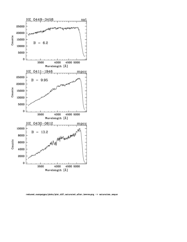
Figure 1.— Spectra displaying a sequence of saturation levels occurring in the survey. For comparison purposes, the three stars have been chosen to have similar color ($B-V\sim 0.45$). Saturation of the emulsion depends on the brightness of the object and the individual photographic plate. Typically, from $\sim 10,000$ counts onwards, the spectra are formed in the non-linear part of the characteristic curve of the photographic emulsion (which slightly varies with each plate). We call these spectra “saturated”. However, as shown in this figure the level of saturation varies and hence the recoverability of the data. The spectrum in the upper panel has been chosen in the visual selection as completely saturated (sat) and was excluded from further processing (for the definitions of the different classes see the text). The middle panel shows a spectrum which has been regarded as recoverable and thus selected as mpcc (see § 2.4). For comparison, an unsaturated spectrum is shown in the lower panel.

Comparison of the $B$ magnitude for the 85 stars in the sample (open circles) with available CCD photometry and the 298 HK calibration stars with photoelectric photometry (crosses). A typical error bar is also shown. As can be seen, the HK calibration sample is fainter than $B\sim 13$ and the agreement with the HES magnitudes is suitable for the search for metal-poor stars. However, no information could be gained concerning the magnitude quality of the brighter stars. This was only achieved after medium-resolution follow-up observations. The additional photometric data of brighter stars revealed that the HES magnitude measurements are somewhat influenced by the saturation effects. The accuracy of the magnitudes was considered sufficient for our current work.

Comparison of the KP index for all sample stars on the photographic plates and in the medium-resolution follow-up spectra. The measurement accuracy of the survey index is clearly affected by saturation of the spectra of stars with $B<13$. A typical error bar is shown in the bottom panel. See text for further details.

Comparison of CCD/photoelectric and survey $B-V$ colors as a function of brightness. Symbols are the same as in Figure Bright Metal-Poor Stars from the Hamburg/ESO Survey. I. Selection and Follow-up Observations from 329 Fields. The scatter becomes much larger for stars brighter that $B=13$, which reflects the onset of saturation effects in the spectra of these objects. A typical error bar is shown for the fainter stars.

Examples of objective-prism spectra (left panel) of the four different classes of metal-poor candidates and their corresponding medium-resolution follow-up spectra (right panel). From the top: classes mpcc, mpcb, unid and mpca. In the insets we show an expansion of the Ca II K region by which the survey spectra were classified. For further description of the classes, see text. We list the telescope employed at the top right corner. The KP and HP2 index, the $(B-V)_{0}$ color and the final iron abundance of each star are shown next to the follow-up spectra (see § 3.2 for more details on the indices). Despite the classification, there is no strong correlation between iron abundance and class.

$B$ magnitude distribution for the bright HES stars, the HK survey stars and the faint HES stars. The magnitude ranges of the samples complement each other and span a large range, from $B\sim 9$ to $B\sim 18$. Top panel: Note that the bimodal distribution of the bright and faint HES stars is due to a selection bias in the sample of bright HES stars (see text for details). Bottom panel: Same distribution as above, but the displayed stars are confirmed to have $\mbox{[Fe/H]}<-2.0$ by follow-up spectroscopy, and randomly selected such that the total numbers of HK survey stars, bright HES and faint HES stars are the same (i.e., 150). Note the smooth distribution, and the removal of the strong selection bias towards bright stars in the sample of bright HES stars that can be seen in the top panel.

$B-V$ color distribution for the bright metal-poor candidate sample as derived from the 2MASS $J-K$ data. When selecting the sample from the HES database, a temperature cut-off at $B-V=0.3$ has been made, based on the original HES colors. Due to the new colors, a few stars now have $B-V<0.3$ which is slightly hotter than has been regarded useful for our search. It is interesting to note here that the sample selected on the basis of the HES colors was originally thought to contain mostly giants. The new $B-V$ colors distribution suggests that the majority of the sample stars are dwarfs and field horizontal branch stars. This color shift is also reflected in Figure Bright Metal-Poor Stars from the Hamburg/ESO Survey. I. Selection and Follow-up Observations from 329 Fields.

Metallicity distribution (MDF) of some 4700 HK survey (upper panel) stars compared to our 293 metal-poor stars (lower panel). See text for discussion.

Sequence of spectra of GP-strong stars. Top panel: The only CH feature visible is the G-band at $\sim 4300$ Å. Middle panel: In addition to the G-band, strong CN molecular bands ($3883$ and $4215$ Å) are also present. These are already clearly visible in the survey spectrum. Bottom panel: The features are even stronger and C₂ bands become visible at e.g., $4738$ and $5165$ Å.

[C/Fe] for all stars with $\mbox{[Fe/H]}<-1.0$ as a function of [Fe/H]. An increased spread of [C/Fe] with decreasing metallicity is clearly seen.

Cumulative frequency of CEMP objects amongst metal-poor stars as function of the distance from the Galactic Plane $Z$. Note that the cumulative fraction is defined as the number of C-enhanced objects amongst metal-poor stars further from the Plane than the indicated $Z$. Top panel: The frequencies for both our and the BPSII sample. Middle panel: Combined data set with $\mbox{[Fe/H]}<-2.0$, overplotted with Poisson errorbars. Bottom panel: Same as middle panel, but for subset of stars with $\mbox{[Fe/H]}<-3.0$. See text for discussion.

Cumulative percentages of normal metal-poor (top curve) and CEMP stars (bottom curve) as a function of distance from the Galactic Plane $Z$. Based on the K–S test, the two samples come from different populations for $Z\gtrsim 2$ kpc. See text for discussion.

Comparison of our final metallicity estimates for rediscovered stars with values derived from medium- (filled circles) and high-resolution (open circles) spectra available in the literature (see Table 3 and text for further details).

Example of an emission-line object found in our sample. As CS 31077-034, this star was classified by Beers et al. (1996a) to have “moderate” Ca II H and K emission.

References

- Anthony-Twarog et al. (2000) Anthony-Twarog, B. J., Sarajedini, A., Twarog, B. A., & Beers, T. C. 2000, AJ, 119, 2882
- Aoki et al. (2006) Aoki, W., Frebel, A., Christlieb, N., Norris, J. E., Beers, T. C., Minezaki, T., Barklem, P. S., Honda, S., Takada-Hidai, M., Asplund, M., Ryan, S. G., Tsangarides, S., Eriksson, K., Steinhauer, A., Deliyannis, C. P., Nomoto, K., Fujimoto, M. Y., Ando, H., Yoshii, Y., & Kajino, T. 2006, ApJ, 639, 897
- Aoki et al. (2001) Aoki, W., Ryan, S. G., Norris, J. E., Beers, T. C., Ando, H., Iwamoto, N., Kajino, T., Mathews, G. J., & Fujimoto, M. Y. 2001, ApJ, 561, 346
- Aoki et al. (2002) Aoki, W., Ryan, S. G., Norris, J. E., Beers, T. C., Ando, H., & Tsangarides, S. 2002, ApJ, 580, 1149
- Barbuy et al. (1997) Barbuy, B., Cayrel, R., Spite, M., Beers, T. C., Spite, F., Nordstroem, B., & Nissen, P. E. 1997, A&A, 317, L63
- Barklem et al. (2005) Barklem, P. S., Christlieb, N., Beers, T. C., Hill, V., Bessell, M. S., Holmberg, J., Marsteller, B., Rossi, S., Zickgraf, F.-J., & Reimers, D. 2005, A&A, 439, 129
- Beers (1999) Beers, T. C. 1999, in ASP Conf. Ser. 165: The Third Stromlo Symposium: The Galactic Halo, ed. B. K. Gibson, R. S. Axelrod, & M. E. Putman, 202
- Beers (2000) Beers, T. C. 2000, in The First Stars. Proceedings of the MPA/ESO Workshop held at Garching, Germany, 3
- Beers et al. (1994) Beers, T. C., Bestman, W., & Wilhelm, R. 1994, AJ, 108, 268
- Beers & Christlieb (2005) Beers, T. C. & Christlieb, N. 2005, ARA&A, 43, 531
- Beers et al. (1985) Beers, T. C., Preston, G. W., & Shectman, S. A. 1985, AJ, 90, 2089
- Beers et al. (1992) —. 1992, AJ, 103, 1987
- Beers et al. (1999) Beers, T. C., Rossi, S., Norris, J. E., Ryan, S. G., & Shefler, T. 1999, AJ, 117, 981
- Beers et al. (1996a) Beers, T. C., Rossi, S., Ulrich, D., & Wilhelm, R. 1996a, AJ, 112, 1188
- Beers et al. (1996b) Beers, T. C., Wilhelm, R., Doinidis, S. P., & Mattson, C. J. 1996b, ApJS, 103, 433
- Bessell & Norris (1984) Bessell, M. S. & Norris, J. 1984, ApJ, 285, 622
- Bessell et al. (1991) Bessell, M. S., Sutherland, R. S., & Ruan, K. 1991, ApJ, 383, L71