Asteroseismic Diagnostics of Stellar Convective Cores

Abstract

We present a detailed study of the small frequency separations as diagnostics of the mass of the convective core and evolutionary stage of solar-type stars. We demonstrate how the small separations can be combined to provide sensitive tests for the presence of convective overshoot at the edge of the core. These studies are focused on low degree oscillation modes, the only modes expected to be detected in distant stars. Using simulated data with realistic errors, we find that the mass of the convective core can be estimated to within 5% if the total stellar mass is known. Systematic errors arising due to uncertainty in the mass could be up to 20%. The evolutionary stage of the star, determined in terms of the central hydrogen abundance using our proposed technique, however, is much less sensitive to the mass estimate.

1 Introduction

The theory of stellar structure predicts that the central region of massive stars ($M\geq 1.1M_{\odot}$) are convective, rather than radiative as is the case for the Sun. Since convective flows imply chemical mixing, the evolution of these stars is severely influenced by the presence, and the extent, of the convective core. The process of convective transport also involves the question of overshoot which implies the extension of the convective region beyond the classical border of convective stability. This causes more hydrogen to be supplied to the nuclear reactions going on in the core, thus effectively increasing the lifetime of a star on the main sequence. The present theories of convection are inadequate to provide a definite measure of the extent of overshoot and it is one of the free parameters in a stellar model. The uncertainty in the mass of the convective core, or its extension due to overshoot, directly translates into an error in the determination of the age of the star. This in turn would affect other studies based on stellar evolution like population synthesis in galaxies etc.

Figure 1: The hydrogen profile near the boundary of the convective core is shown for a $1.3M_{\odot}$ model with overshoot at different stages of evolution. The flat portion of the curve indicates the core which is fully mixed due to convection. It is clear that the size of the core increases during the first part of evolution before shrinking in later stages. Diffusion of hydrogen leaves a smoothed out step-like signature in the hydrogen profile as the core recedes with increasing age of the star.

The size of the convective core does not remain constant, and changes as the star evolves. The variation in the core size of a $1.3M_{\odot}$ star is illustrated in Fig. 1 through the change in the hydrogen profile as a function of fractional mass. For stars of mass $1.1\leq M/M_{\odot}\leq 2.0$ the core increases in size during the initial stages of evolution before beginning to shrink later. Furthermore, stellar models indicate that the extent and evolution of the convective core is quite different depending on whether or not convective overshoot is present (Fig. 2). It is, therefore, clear that a good test of the presence and extent of convective layers in the central region of massive stars will go a long way towards our understanding of stellar structure and evolution. While there is no direct method to look inside a star, the recent advances in asteroseismology does offer an opportunity to probe the innermost layers of stars. The frequencies of oscillation of a star depend on its global properties like the mass, radius etc, as well as the detailed internal structure, especially the location of layers of rapid change in density or chemical composition, and hence can be used to probe the inner layers.

Space-based asteroseismic missions such as MOST (Walker et al. 2003) and CoRoT (Baglin 2003) are expected to measure the oscillation frequencies of several stars with sufficient accuracy to enable a more detailed study of stellar structure than has been possible so far. Ground-based observations have already started measuring the frequencies of many stars despite the difficulties of such measurements. Unfortunately, none of these observations can or will be able to observe the intermediate degree modes of oscillation that have been so useful in solar studies. These missions can at most, hope to determine the frequencies of modes with degree $\ell\leq 3$. However, we are fortunate in the fact that the modes of low degrees ($\ell=0$–$3$) penetrate the central regions of a star and hence carry information about its deepest layers. We focus our study only on these modes.

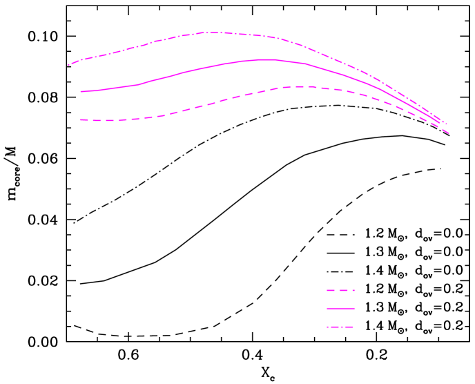
Figure 2: The evolution of the fractional mass of the convective core, $m_{\mathrm{core}}/M$ is shown for models of mass $1.2$, $1.3$ and $1.4M_{\odot}$. The black lines represent models without convective core overshoot and the other curves show models in which core overshoot ($0.2H_{P}$) has been incorporated.

It has been suggested that the oscillatory signal in the frequencies due to sharp features such as the boundaries of convective regions or ionisation zones can be used to estimate the location of these layers inside a star (Monteiro et al. 1998, 2000). While this technique appears to succeed for the base of the outer convective envelope or the second helium ionisation zone (Ballot et al. 2004; Basu et al. 2004), Mazumdar & Antia (2001) have shown that it would not work for the convective core due to a problem similar to aliasing in Fourier analysis. In this paper we show that combinations of frequency separations can provide a better knowledge of the core.

It is well known that the large scale properties like the mass and radius act mostly to scale the frequencies of nearly all modes of oscillation. Such scaling effects are apparent in the large separation, i.e., the difference in frequency of modes of successive order but of a particular degree. The large separations are also quite sensitive to the structure of the outer layers of a star, which are among the most uncertain aspects of theoretical stellar models. On the other hand, the so-called small separations, i.e., the small differences of frequency between modes of nearly same order but different degrees, are more affected by the deeper layers of a star. Therefore, the small separations are useful in investigating the central features, especially the extent of convective cores in massive stars.

Indeed, many efforts have been made to link the small frequency separations to the convective core in massive stars (for theoretical studies see, e.g., Dziembowski & Pamyatnykh 1991; Roxburgh & Vorontsov 2001). Using $\alpha$ Cen models, Guenther & Demarque (2000) had suggested to use the small separations to constrain the age of the stars. After oscillations were indeed detected in $\alpha$ Cen AB (Bouchy & Carrier 2002; Carrier & Bourban 2003; Bedding et al. 2004; Kjeldsen et al. 2005), different authors have made use of the small separations to constrain the parameters, especially the age, for these stars (Thévenin et al. 2002; Thoul et al. 2003; Eggenberger et al. 2004). Recently, Roxburgh & Vorontsov (2003) have demonstrated that the ratio of the small and large separations serve as a better diagnostic of the innermost layers of a star than the small separations alone. Miglio & Montalbán (2005) have used this technique to refine the seismic models for $\alpha$ Cen AB. Similarly, the small separations have proved to be useful for the seismic modelling of Procyon A as well (Eggenberger et al. 2005; Provost et al. 2006). Straka et al. (2005) have provided upper limits to the convective overshoot in Procyon A models using the frequency separations. In these studies, the frequency separations have been mostly used to find the best possible model that fits the observed data for a given star. In this paper we aim to present a general technique for probing specific properties of the central regions of a star, like the mass of the convective core, and the state of evolution of the star, using suitable combinations of the frequency separations.

While the large and small separation corresponding to each radial order encodes information about a different layer inside the star, and is, therefore, an independent diagnostic of the structure, there are also advantages in considering suitable average values of these separations. Firstly, the averaging over several radial orders removes the small-scale variations due to subtle differences in the internal structure, and enhances the effects of the more significant features of the stellar interior. Second: it is often not possible from observations to determine the frequency of modes of all radial orders for the same degree, and an average is often the best indication of the trend of frequencies. Third: while individual frequencies, and hence the separations are often susceptible to large observational errors, the average values of the large and small separations turn out to be robust quantities (Mazumdar 2005). The diagnostic power of the average separations can be utilised very well through the Christensen-Dalsgaard diagram (Christensen-Dalsgaard 1988) to determine the mass and age of a star. In this work, we show that they can also be used for more detailed study of the stellar interior and present a practical method involving the average values of small and large separations and combinations thereof to estimate the age of a star and the mass of the convective core.

In the next section we define new diagnostic quantities to probe the stellar core and outline our technique and describe the stellar models used in this work. Our results along with error estimates are presented in Section 3 with the concluding discussion in Section 4.

2 The Technique

The average large separation of radial modes is defined as

$$\Delta=\langle\nu(n+1,0)-\nu(n,0)\rangle,$$ (1)

where the angular brackets imply averaging over a range of radial order, $n$, appropriately chosen.

The small separation between modes of degree $\ell$ and $\ell+2$ is defined as

$$\delta_{\ell\,\ell+2}(n)=\nu(n,\ell)-\nu(n-1,\ell+2)$$ (2)

While comparing small separations between different pairs of modes (e.g., $(\ell=0,2)$ and $(\ell=1,3)$) it is convenient to scale the differences to eliminate the factor of $\ell(\ell+1)$ in the frequencies. Thus one may define the scaled small separations as (cf.  Christensen-Dalsgaard & Berthomieu 1991; Roxburgh & Vorontsov 2001)

$$D_{\ell\,\ell+2}(n)=\frac{\delta_{\ell\,\ell+2}(n)}{4\ell+6}=\frac{\nu(n,\ell)-\nu(n-1,\ell+2)}{4\ell+6}$$ (3)

In the rest of the paper, we will refer to this scaled definition, $D_{\ell\,\ell+2}$, simply as the “small separation”. The small separation between modes of degree $\ell=0$ and 2 are designated as $D_{02}$, and those corresponding to $\ell=1$ and 3 as $D_{13}$. Roxburgh & Vorontsov (2001) have demonstrated that these two sets of small separations encode similar, but somewhat different information about the central layers. This is explained by the fact that modes of different degree have different inner turning points, and therefore probe different layers. Thus, it might be useful to compare the two small separations, $D_{02}(n)$ and $D_{13}(n)$, of the same radial order.

In order to exploit the fine differences between $D_{02}(n)$ and $D_{13}(n)$, for each model, we define the following combinations of the small separations:

$$\theta(n_{1},n_{2})=\frac{\Delta_{\odot}}{\Delta}\,\left\langle D_{13}(n)-D_{02}(n)\right\rangle_{n=n_{1}\,\mathrm{to}\,n_{2}}$$ (4)

$$\eta(n_{1},n_{2})=\left(\frac{\Delta_{\odot}}{\Delta}\right)^{2}\,\left\langle(D_{13}(n)-D_{02}(n))^{2}\right\rangle_{n=n_{1}\,\mathrm{to}\,n_{2}}$$ (5)

where the arguments $n_{1}$ and $n_{2}$ indicate the limits of radial orders between which the averaging is carried out. $\Delta_{\odot}$ is the average large separation of the Sun ($\Delta_{\odot}\simeq 135\mu$Hz).

The properties of the quantities $\theta$ and $\eta$, and their sensitivity to different stellar parameters, would partly depend on the range of the radial order chosen for averaging. We deliberately choose relatively higher order modes ($n\geq 10$) for averaging to avoid contamination from mixed modes. In practice, however, the choice of the range for averaging would be primarily governed by the availability of data in different frequency ranges of the observed spectrum. For a complete set of frequencies of a solar-type star, we find that the range of $n=15$ to $28$ for $\theta$ and $n=10$ to $28$ for $\eta$ make these quantities ideally sensitive to stellar properties such as the convective core mass, $m_{\mathrm{core}}$ or the central hydrogen abundance, $X_{\mathrm{c}}$. In the rest of the paper, we shall assume these to be the respective ranges of averaging for $\theta$ and $\eta$, unless the range is stated explicitly.

We include the scaling factors $\Delta_{\odot}/\Delta$ in the definitions of $\theta$ and $\eta$ to reduce homology effects while comparing stars of different mass and radius. This factor essentially filters out the global scaling of the frequencies due to differences in the mean density of different stars, and enhances the effects of the structural details which we want to study.

We study the variation of these new diagnostic quantities, $\theta$ and $\eta$ with the age and evolution of the convective core in stars using a large number of stellar models. We restrict ourselves to stars with masses just a little higher than the mass of the Sun, namely, the range 1.2–1.4$M_{\odot}$. We study stellar models evolved to different ages on the main sequence for masses $1.2$, $1.3$ and $1.4M_{\odot}$. Ideally, the boundary of the growing convective core should be tracked by adjusting the mesh at each evolutionary step. However, since the current evolutionary code does not have that capability, the edge of the core is determined through the Schwarzschild criterion being tested over a very fine mesh in the central regions of the star. To compare with stars without convection in their cores, we also constructed a sequence of $1M_{\odot}$ models. We also vary the convective overshoot in the core, which is measured in units of the local pressure scale height, $H_{P}$. We use two sets of models with the overshoot parameter $d_{\mathrm{ov}}=0$ and $d_{\mathrm{ov}}=0.2$, where the amount of overshoot at the edge of the convective core is given by $d_{\mathrm{ov}}H_{P}$. For very small convective cores, the overshoot is limited to be a fraction of the core size instead of $H_{P}$. However, for most of the models that we consider, the size of the core is typically at least an order of magnitude larger than the pressure scale height at the boundary, so that we can simply use $d_{\mathrm{ov}}H_{P}$ as a measure of the overshoot.

The models used in this work were constructed using YREC, the Yale Rotating Evolution Code in its non-rotating configuration (Guenther et al. 1992). These models use the OPAL equation of state (Rogers & Nayfonov 2002), OPAL opacities (Iglesias & Rogers 1996), low temperature opacities of Alexander & Ferguson (1994) and nuclear reaction rates as used by Bahcall & Pinsonneault (1992). The models take into account diffusion of helium and heavy elements, using the prescription of Thoul et al. (1994). The initial chemical composition of the models was fixed at $(Y_{0}=0.26,Z_{0}=0.022)$.

3 Results

3.1 Testing for core overshoot

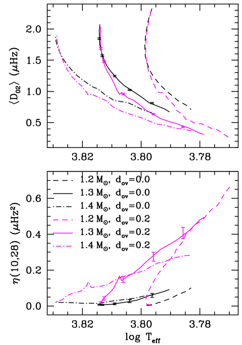
Figure 3: The evolution of the average small separation $\langle D_{02}\rangle$ (upper panel) and the new diagnostic $\eta$ (lower panel) as a function of the effective temperature are shown. The black lines represent models without overshoot while the other lines represent models with overshoot ($d_{\mathrm{ov}}=0.2$). For each mass the curves for models with and without overshoot diverge from the zero age main sequence. The errorbars represent $1\sigma$ errors in the respective quantities for relative frequency errors of $10^{-4}$, obtained through simulations described in Section 3.4.1. The significant kink in the curves, especially for overshoot models, correspond to the age of the star when the convective core stops expanding and begins shrinking.

As is clear from Fig. 2 the evolution of the central convective region of a star with age is significantly affected by the presence of overshoot. Indeed, we find that this important difference is reflected in the oscillation frequencies and consequently, the small separations. The presence of convective overshoot, therefore, might be tested through the small separations themselves. Di Mauro et al. (2003) have made a detailed investigation on how the frequency separations can be used to distinguish between models with and without overshoot for a post-main sequence star. Mazumdar (2005), however, has shown that during the main sequence phase the direct effect of overshoot on the small separations $D_{02}$ becomes noticeable only in the later stages of evolution. We investigate whether the average small separations, $\langle D_{02}\rangle$, or the quantity $\eta$ can provide any clue to the presence of overshoot in a given star.

In Fig. 3, we show how the average small separations $\langle D_{02}\rangle$ and the quantity $\eta$ vary as functions of the effective temperature as the star evolves on the main sequence, for models with and without core overshoot. The errorbars represent the $1\sigma$ errors in the ordinates for relative frequency errors of $10^{-4}$. These errorbars were obtained from Monte Carlo simulations with theoretical frequencies, described in detail in Section 3.4.1. It is evident that even if the mass of a star is known, $\langle D_{02}\rangle$ is barely sufficient to distinguish between models with and without overshoot at a given $T_{\mathrm{eff}}$. The tracks for $\eta$, on the other hand, are well separated, with the overshoot models producing much higher values of $\eta$ at a given $T_{\mathrm{eff}}$, irrespective of mass. While the $\langle D_{02}\rangle$ values for models with and without overshoot are nearly the same, especially near the zero age main sequence (ZAMS), the $\eta$ values of overshoot models diverge very rapidly beyond the ZAMS from those of non-overshoot models. Thus, if the location of a star on the HR diagram is known, the quantity $\eta$ can be used to test the presence of overshoot in the convective core. For large errors in frequency the errors in $\eta$ increase almost linearly (see Table 1); even for relative errors $5\times 10^{-4}$ the separation between the tracks is large enough to be distinctive to prove useful.

3.2 Estimating the convective core mass, $m_{\mathrm{core}}$

Figure 4: The scaled mass of the convective core, $(\Delta_{\odot}/\Delta)^{2}m_{\mathrm{core}}/M$ is plotted as a function of the average small separation, $\langle D_{02}\rangle$, for models without overshoot (upper panel) and with overshoot (lower panel). The dotted line shows the $\langle D_{02}\rangle$ values for a $1M_{\odot}$ model, for which the core is not convective. The errorbars represent $1\sigma$ errors in $\langle D_{02}\rangle$ for relative frequency errors of $10^{-4}$, obtained through simulations described in Section 3.4.1. The significant kink in the curves, especially for overshoot models, correspond to the age of the star when the convective core stops expanding and begins shrinking.

Figure 5: The scaled mass of the convective core, $(\Delta_{\odot}/\Delta)^{2}m_{\mathrm{core}}/M$ is plotted as a function of the diagnostic, $\eta$, for models without overshoot (upper panel) and with overshoot (lower panel). The dotted line shows the $\eta$ values for a $1M_{\odot}$ model, for which the core is not convective. The errorbars represent $1\sigma$ errors in $\eta$ for relative frequency errors of $10^{-4}$, obtained through simulations described in Section 3.4.1. The significant kink in the curves, especially for overshoot models, correspond to the age of the star when the convective core stops expanding and begins shrinking.

As evident from Figs. 1 and 2, the fractional mass of the convective core of a star of total mass of about $1.2$–$1.4$$M_{\odot}$ does not remain constant throughout its main sequence evolution. In particular, the convective core grows during the early part of evolution and then begins to shrink at later stages. The exact evolution of the core depends somewhat on the total mass and quite strongly on whether or not convective overshoot occurs. In either case, the relationship between the fractional mass of the core and the age of the star has opposite signs in two parts of evolution on the main sequence. Since the mass of the convective core is not monotonic with the age, it is difficult to associate the core mass directly with the small separations (and hence with $\theta$ or $\eta$), which vary generally monotonically with age. However, we find that if we scale the mass of the core with the factor $(\Delta_{\odot}/\Delta)^{2}$ which is related to the mean density of the star, the scaled mass is nearly monotonic with the age of the star. Of course, even this scaled mass of the core eventually decreases with increasing age towards the end of the main sequence when the core shrinks to a very small size. While theoretically this might appear to be somewhat ad hoc, it provides a practical way to overcome the difficult dichotomy of the core mass. Observationally, it is a perfectly suitable method since the average large separation can usually be measured to a fair degree of accuracy. If the scaled core mass can be determined using a seismic diagnostic, the actual mass of the core can easily be extracted through the average large separation.

We have also found from Fig. 3 that the value of $\eta$ is strongly dependent on the presence of overshoot. This implies that we need separate calibration curves for models with and without core overshoot. Since Fig. 3 itself provides a means of testing for the presence of overshoot, from a practical viewpoint, this does not pose a problem while dealing with a given star. We use multiple models at different ages of $1.2$, $1.3$ and $1.4M_{\odot}$ both with and without overshoot to produce the needed calibration curves.

We first investigate the variation of the average small separation, $\langle D_{02}\rangle$ with the scaled fractional core mass, $(\Delta_{\odot}/\Delta)^{2}m_{\mathrm{core}}/M$. In Fig. 4 we show the scaled core mass as function of $\langle D_{02}\rangle$, for stellar models of different mass, evolving through the main sequence. Every curve in this figure is an evolutionary track, which serves as a calibration curve to determine $(\Delta_{\odot}/\Delta)^{2}m_{\mathrm{core}}/M$ for a given target. The figure (and similarly Figs 5, 6 and 7) have been drawn such that the sense of evolution is from the left to the right along the $x$-axis.

This figure illustrates the fact that although models with the same core mass have largely different values of the small separation, the scaled core mass is almost monotonic with $\langle D_{02}\rangle$. It is worth mentioning that the kink in the curves shown in the lower panel of Fig. 4 is not an artifact of the stellar models. It is, in fact, intrinsic to the evolution of the star, and corresponds to the age when the increase of the core size stops and the core begins to shrink (cf. Fig. 2). Such a kink is also seen in the Christensen-Dalsgaard diagrams (Mazumdar 2005). The presence of the kink implies that a careful calibration needs to be carried out – perhaps two different calibrations for two segments of the evolutionary track. For comparison, we have also plotted the $\langle D_{02}\rangle$ values for a $1M_{\odot}$ model, which does not have a convective core at all. Every horizontal errorbar indicates the $1\sigma$ error in $\langle D_{02}\rangle$ due to relative frequency errors of $10^{-4}$, which would translate into a random error in the determination of $(\Delta_{\odot}/\Delta)^{2}m_{\mathrm{core}}/M$ through the local slope of the calibration curves. Given the wide separation of the curves corresponding to different masses, it is clear that such random error in estimating the core mass due to errors in frequencies is much smaller than the uncertainty due to the stellar mass. Therefore, to use this technique, one needs to have a fair idea of the mass of the star. We shall investigate both the random and systematic errors involved in detail in Sections 3.4.1 and 3.4.2 respectively.

Figure 6: The central hydrogen abundance, $X_{\mathrm{c}}$ is plotted as a function of the diagnostic, $\eta$, for models without overshoot (upper panel) and with overshoot (lower panel). The errorbars represent $1\sigma$ errors in $\eta$ for relative frequency errors of $10^{-4}$, obtained through simulations described in Section 3.4.1. The significant kink in the curves, especially for overshoot models, correspond to the age of the star when the convective core stops expanding and begins shrinking. For the no-overshoot models $\eta$ is poorly sensitive to $X_{\mathrm{c}}$ at early stages of evolution and hence it will not be possible to determine $X_{\mathrm{c}}$ for low values of $\eta$.

Figure 7: The central hydrogen abundance, $X_{\mathrm{c}}$ is plotted as a function of the diagnostic, $\theta$, for models without overshoot (upper panel) and with overshoot (lower panel). The errorbars represent $1\sigma$ errors in $\theta$ for relative frequency errors of $10^{-4}$, obtained through simulations described in Section 3.4.1. It turns out that the correlation of $\theta$ with $X_{\mathrm{c}}$ becomes poor beyond a certain evolutionary stage (depending on the mass) and the curves are truncated only to show the part that would be usable for the determination of $X_{\mathrm{c}}$.

We can also use the quantity $\eta$ as an additional diagnostic for the convective core. The variation of $\eta$ with $(\Delta_{\odot}/\Delta)^{2}m_{\mathrm{core}}/M$ is illustrated in Fig. 5. We find that $\eta$ is more sensitive to the core mass in the presence of overshoot. Actually, the use of $\eta$ as a diagnostic is restricted only to more evolved models in the absence of overshoot, especially for the $1.4M_{\odot}$ models. The presence of the kink again implies that for stars near that particular evolutionary stage the error in the core mass estimate will be larger. We also note that unlike $\langle D_{02}\rangle$, the range of values of $\eta$ for a star without a convective core, the $1M_{\odot}$ model, is restricted to much smaller values than that for stars with a convective core. This is one advantage that $\eta$ has, as a diagnostic of $m_{\mathrm{core}}$, over $\langle D_{02}\rangle$ (cf. Fig. 4).

3.3 Estimating $X_{\mathrm{c}}$

The central parts of a star change more rapidly than the outer layers with age. Thus, it is not surprising that the small separations, or combinations thereof, can be used as indicators of stellar age (Christensen-Dalsgaard 1988). We have investigated how sensitive the quantities $\eta$ and $\theta$ are to the stellar age, as measured in terms of the central hydrogen abundance, $X_{\mathrm{c}}$. Figs. 6 and 7 show the calibration curves. As with the core mass, we find that in the absence of overshoot $\eta$ is not very sensitive to $X_{\mathrm{c}}$ either. For overshoot models, however, $\eta$ may be used as an indicator of $X_{\mathrm{c}}$ throughout the main sequence phase, provided the mass is independently known. The quantity, $\theta$, on the other hand, serves as a good diagnostic for $X_{\mathrm{c}}$ in the early stages of evolution. Beyond a certain age, which depends slightly on the mass, $\theta$ no longer follows a regular pattern with $X_{\mathrm{c}}$. At younger ages, however, $\theta$ is less sensitive to the stellar mass, which would make it an excellent indicator of the evolutionary stage if the mass is not well-constrained. The quantities $\theta$ and $\eta$ also serve as complementary diagnostics of $X_{\mathrm{c}}$ at different stages of evolution.

3.4 Errors in estimation of $m_{\mathrm{core}}$ and $X_{\mathrm{c}}$

3.4.1 Random errors

Figure 8: The mass of the convective core, as determined through the calibration of $(\Delta_{\odot}/\Delta)^{2}m_{\mathrm{core}}/M$ vs $\langle D_{02}\rangle$ (Fig. 4), is plotted against the model value. Results are shown for test models both without (upper panel) and with (lower panel) overshoot. In each case, the calibration curve corresponding to the same mass and overshoot was used. The dotted lines show the values which would be obtained for a perfect match with the model. The errorbars show the ${\mathbf{3}}\sigma$ error estimates for relative frequency errors of $10^{-4}$.

Figure 9: The mass of the convective core, as determined through the calibration of $(\Delta_{\odot}/\Delta)^{2}m_{\mathrm{core}}/M$ vs $\eta$ (Fig. 5), is plotted against the model value. Results are shown for test models both without (upper panel) and with (lower panel) overshoot. In each case, the calibration curve corresponding to the same mass and overshoot was used. The dotted lines show the values which would be obtained for a perfect match with the model. The errorbars show the ${\mathbf{3}}\sigma$ error estimates for relative frequency errors of $10^{-4}$.

Table 1: Results of Monte Carlo simulations of determination of $m_{\mathrm{core}}$ and $X_{\mathrm{c}}$ for 5 test models at different ages with mass $M=1.3M_{\odot}$ and overshoot $d_{\mathrm{ov}}=0.2$ are shown. For each model the top row shows the original input model values. The three subsequent rows show the results for different quantities when relative errors in frequency of $1\times 10^{-4}$, $5\times 10^{-4}$ and $1\times 10^{-3}$ respectively are added to the model frequencies. In each case, the results represent the average and $1\sigma$ errors for 100 independent realisations of the simulated data. The blank entries indicate that the technique fails to extract the desired quantity either due to lack of sensitivity of the diagnostic, or too high an error in frequencies to use the calibration curves.

Age	$\Delta$		$\langle D_{02}\rangle$		$\theta$		$\eta$		$m_{\mathrm{core}}/M$				$X_{\mathrm{c}}$
									using		using		using		using
(Gyr)	($\mu$Hz)		($\mu$Hz)		($\mu$Hz)		($\mu$Hz2)		$\langle D_{02}\rangle$		$\eta$		$\eta$		$\theta$
1.300	108.862		1.689		0.093		0.020		0.083				0.604
	108.863$\pm$	0.017	1.689$\pm$	0.014	0.094$\pm$	0.025	0.026$\pm$	0.005	0.084$\pm$	0.001	0.088$\pm$	0.003	0.585$\pm$	0.012	0.602$\pm$	0.014
	108.869$\pm$	0.086	1.688$\pm$	0.067	0.099$\pm$	0.126	0.171$\pm$	0.052	0.084$\pm$	0.003	0.143$\pm$	0.018	0.394$\pm$	0.063	0.599$\pm$	0.070
	108.876$\pm$	0.173	1.687$\pm$	0.134	0.106$\pm$	0.252	0.620$\pm$	0.195	0.084$\pm$	0.007	– –		– –		0.578$\pm$	0.096
1.885	102.054		1.477		0.212		0.042		0.086				0.544
	102.055$\pm$	0.016	1.477$\pm$	0.012	0.213$\pm$	0.025	0.048$\pm$	0.009	0.084$\pm$	0.001	0.087$\pm$	0.004	0.540$\pm$	0.018	0.536$\pm$	0.014
	102.060$\pm$	0.081	1.475$\pm$	0.062	0.216$\pm$	0.126	0.195$\pm$	0.070	0.084$\pm$	0.004	0.131$\pm$	0.017	0.370$\pm$	0.074	0.539$\pm$	0.066
	102.067$\pm$	0.162	1.474$\pm$	0.124	0.221$\pm$	0.251	0.650$\pm$	0.234	0.085$\pm$	0.007	– –		– –		0.576$\pm$	0.092
3.000	88.636		0.957		0.408		0.148		0.092				0.411
	88.637$\pm$	0.014	0.957$\pm$	0.011	0.409$\pm$	0.025	0.156$\pm$	0.017	0.088$\pm$	0.001	0.090$\pm$	0.008	0.420$\pm$	0.037	0.435$\pm$	0.010
	88.642$\pm$	0.070	0.956$\pm$	0.055	0.414$\pm$	0.126	0.304$\pm$	0.098	0.090$\pm$	0.005	0.112$\pm$	0.011	0.281$\pm$	0.080	– –
	88.648$\pm$	0.141	0.955$\pm$	0.109	0.421$\pm$	0.252	0.759$\pm$	0.258	0.091$\pm$	0.009	– –		– –		– –
3.855	78.129		0.636		0.505		0.275		0.089				0.280
	78.130$\pm$	0.013	0.636$\pm$	0.010	0.506$\pm$	0.026	0.282$\pm$	0.025	0.088$\pm$	0.001	0.088$\pm$	0.002	0.286$\pm$	0.022	– –
	78.134$\pm$	0.062	0.635$\pm$	0.048	0.510$\pm$	0.128	0.433$\pm$	0.133	0.088$\pm$	0.002	0.092$\pm$	0.006	0.223$\pm$	0.068	– –
	78.139$\pm$	0.124	0.635$\pm$	0.097	0.515$\pm$	0.255	0.897$\pm$	0.322	0.089$\pm$	0.004	– –		– –		– –
4.400	71.480		0.428		0.550		0.407		0.080				0.173
	71.481$\pm$	0.011	0.428$\pm$	0.009	0.552$\pm$	0.026	0.415$\pm$	0.032	0.081$\pm$	0.001	0.080$\pm$	0.001	0.163$\pm$	0.018	– –
	71.485$\pm$	0.057	0.427$\pm$	0.046	0.557$\pm$	0.130	0.569$\pm$	0.177	0.080$\pm$	0.001	– –		– –		– –
	71.490$\pm$	0.114	0.426$\pm$	0.093	0.562$\pm$	0.260	1.040$\pm$	0.431	0.080$\pm$	0.001	– –		– –		– –

Having constructed calibration curves for the core mass and stellar age, the next step is to check whether we can use them for real data with errors. Since at present we do not have enough observational data to test these methods, we undertook a Monte-Carlo simulation where random errors with a Gaussian distribution that has a specified standard deviation were added to the exact frequencies of a given test model. All the necessary separations were then calculated with these error-added frequencies and the desired quantity ($m_{\mathrm{core}}$ or $X_{\mathrm{c}}$) was estimated using the calibration curves. Finally, the averages of the estimates along with errorbars were obtained from 100 such realisations. Typically we used five test models at different evolutionary stages for each mass to check the viability of the method. For each test model, it is assumed that the mass of the target star is known and that the question of overshoot has been settled independently – through a test like Fig. 3, or by some other constraint – so that we can use a calibration curve constructed for the same mass and overshoot. The systematic errors arising due to uncertainties in these respects will be treated separately in the next section.

Figures 8 to 11 show the results of these tests. In each figure we compare the original input model value of $m_{\mathrm{core}}$ and $X_{\mathrm{c}}$ against their estimated values. The errorbars indicate $3\sigma$ errors obtained assuming a constant relative error of 1 part in $10^{4}$ in frequencies. Such errors in frequencies are in line with the expectations from the CoRoT mission. Even recent ground-based observations have reached almost this level of precision (Bouchy & Carrier 2002). For the estimation of $m_{\mathrm{core}}$ we note that the error is introduced at two points – first when we determine the scaled core mass, $(\Delta_{\odot}/\Delta)^{2}m_{\mathrm{core}}/M$, from the calibration curves (Figs. 4 and 5) and then through the average large separation, $\Delta$ to extract $m_{\mathrm{core}}$. The error in $\Delta$ is, however, tiny compared to the contribution from the calibration curves while determining $(\Delta_{\odot}/\Delta)^{2}m_{\mathrm{core}}/M$.

For the set of models with $M=1.3M_{\odot},d_{\mathrm{ov}}=0.2$ we have also tested the method for higher error in the frequencies – relative errors of $5\times 10^{-4}$ and $1\times 10^{-3}$ were added to the frequencies. The results, presented in Table 1, show that the errors are propagated linearly and that the techniques to extract $m_{\mathrm{core}}$ and $X_{\mathrm{c}}$ begin to fail only at the level of $\delta\nu/\nu\simeq 10^{-3}$, which is ten times worse than the precision level expected from CoRoT. However, in some cases where the diagnostic is poorly sensitive to $m_{\mathrm{core}}$ or $X_{\mathrm{c}}$ in a particular phase of evolution (e.g., $\eta$ is a poor indicator of $X_{\mathrm{c}}$ at younger ages), even a small error in the diagnostic would possibly lead to a wrong value of $m_{\mathrm{core}}$ or $X_{\mathrm{c}}$ for a star in that phase of evolution, even if the errorbar remains small. This is what is seen in Table 1, for example, in the $X_{\mathrm{c}}$ values extracted from $\eta$ for relative frequency errors of $5\times 10^{-4}$.

Figure 10: The central hydrogen abundance, as determined through the calibration of $X_{\mathrm{c}}$ vs $\eta$ (Fig. 6), is plotted against the model value. Results are shown for test models both without (upper panel) and with (lower panel) overshoot. In each case, the calibration curve corresponding to the same mass and overshoot was used. The dotted lines show the values which would be obtained for a perfect match with the model. The errorbars show the ${\mathbf{3}}\sigma$ error estimates for relative frequency errors of $10^{-4}$. The technique does not work at younger ages for no-overshoot models due to the lack of sensitivity of $\eta$ to $X_{\mathrm{c}}$ (cf. Fig. 6). The instances of larger errorbars for $1.3$ and $1.4M_{\odot}$ occur when the test model is close to the kink in the calibration curve.

Figure 11: The central hydrogen abundance, as determined through the calibration of $X_{\mathrm{c}}$ vs $\theta$ (Fig. 7), is plotted against the model value. Results are shown for test models both without (upper panel) and with (lower panel) overshoot. In each case, the calibration curve corresponding to the same mass and overshoot was used. The dotted lines show the values which would be obtained for a perfect match with the model. The errorbars show the ${\mathbf{3}}\sigma$ error estimates for relative frequency errors of $10^{-4}$. The technique does not work at low values of $X_{\mathrm{c}}$ due to the non-regular variation of $\theta$ with $X_{\mathrm{c}}$ at more evolved stages (cf. Fig. 7).

3.4.2 Systematic errors

Figure 12: The mass of the convective core of $1.25M_{\odot}$ models, as determined by using the calibration curves of $1.2M_{\odot}$ and $1.3M_{\odot}$, is plotted against the model value. The upper panel shows results obtained using $\langle D_{02}\rangle$, while the lower panel shows results obtained using $\eta$ calibration. The dotted lines indicate the perfect match of the model and extracted values. The errorbars show the random ${\mathbf{3}}\sigma$ errors for relative frequency errors of $10^{-4}$. The unusually large errorbars correspond to the uncertainty introduced by the kink region in the calibration curves (Figs. 4 and 5).

Figure 13: The central hydrogen abundance of $1.25M_{\odot}$ models, as determined by using the calibration curves of $1.2M_{\odot}$ and $1.3M_{\odot}$, is plotted against the model value. The upper panel shows results obtained using $\theta$, while the lower panel shows results obtained using $\eta$ calibration. The dotted lines indicate the perfect match of the model and extracted values. The errorbars show the random ${\mathbf{3}}\sigma$ errors for relative frequency errors of $10^{-4}$.

In applying our technique to determine $m_{\mathrm{core}}$ and $X_{\mathrm{c}}$ of a given target star, we shall need to use calibration curves with approximately the same mass and overshoot as the target. In reality, however, these quantities are never a priori known exactly. Therefore, we need to investigate the extent of systematic errors in $m_{\mathrm{core}}$ and $X_{\mathrm{c}}$ arising due to the use of inexact calibration curves.

The question of overshoot is one that asteroseismology hopes to answer. Straka et al. (2005) have suggested a method of estimating overshoot through the small separations of $g$-modes. In Section 3.1 we have also demonstrated how $\eta$ can be used to detect the presence of core overshoot. For this study, however, we realise that the calibration curves are significantly dependent on overshoot and the systematic errors could indeed be large if an inexact value of core overshoot is used in the calibration ($\sim 40\%$ for an error of $\delta d_{\mathrm{ov}}\simeq 0.2$). Therefore, we conclude that an independent estimate of the core overshoot would be necessary to use our technique to determine $m_{\mathrm{core}}$ and $X_{\mathrm{c}}$ to better accuracy.

For solar-type stars the location on the HR diagram can be determined with a fair accuracy which often provides a reasonable estimate of the mass of the star. Usually, the mass of a solar-type star is known to within $0.10M_{\odot}$ purely from its spectral type and luminosity. We have investigated the systematic errors in $m_{\mathrm{core}}$ and $X_{\mathrm{c}}$ due to uncertainty in the mass by using calibration curves of both $1.2M_{\odot}$ and $1.3M_{\odot}$ for target models of $1.25M_{\odot}$. The results are shown in Figs. 12 and 13. The errorbars in these figures still indicate the random errors due to relative frequency errors of $10^{-4}$. As expected, $m_{\mathrm{core}}$ is systematically underestimated when a lower mass is used for calibration, and vice versa. For an error of $0.05M_{\odot}$ in mass, the systematic error in $m_{\mathrm{core}}/M$ is $\sim 0.015$ on average. Evidently, the systematic errors in $m_{\mathrm{core}}$ are much larger than the random errors arising due to errors in frequencies.

The situation is, however, different for the determination of $X_{\mathrm{c}}$. Fig. 13 shows that $X_{\mathrm{c}}$ can be determined fairly accurately from either $\theta$ (only at younger ages) or $\eta$ even if the mass is not known exactly. Importantly, there is no systematic trend in the error in $X_{\mathrm{c}}$ due to an incorrect estimate of the mass. The random errors actually span the range of uncertainty introduced due to an incorrect estimate of the mass. This is not surprising, given the closeness of the calibration curves for different masses in Figs. 6 and 7.

4 Discussion

We have presented the results of our study to relate the small frequency separations to the central layers of solar-type stars. We have shown that the average small separation, $\langle D_{02}\rangle$, can be used as a measure of the mass of the convective core in stars of mass $1.2$–$1.4M_{\odot}$. In addition, we also propose two combinations, $\theta$ and $\eta$, of the small separations of different pairs of degrees as new diagnostics of the mass of the convective core, $m_{\mathrm{core}}$ and the stellar age, in terms of $X_{\mathrm{c}}$. We have tested the applicability of our technique to data with errors by estimating the random and systematic errors in $m_{\mathrm{core}}$ and $X_{\mathrm{c}}$ through Monte Carlo simulations. The motivation behind the use of such combinations of $D_{02}$ and $D_{13}$ stems from the fact that while they both encode slightly different internal phase shifts (Roxburgh & Vorontsov 2001), their combination might be sensitive to the sharp discontinuity at the boundary of the core. A more thorough theoretical analysis of these diagnostic quantities is required to understand their features better. It turns out that the diagnostic value of $\eta$ and $\theta$ can be maximised with an appropriate choice of the frequency ranges indicated here. A different choice of the frequency range is not only feasible, but might, in fact, be necessary depending on the availability of data. A detailed error analysis using calibration curves with the available observed frequencies to be used for the averaging would, however, be necessary in order to apply the technique to real data.

It turns out that all the calibration curves depend on convective overshoot in the core, and therefore we would need an independent estimate of the extent of overshoot in order to determine $m_{\mathrm{core}}$ and $X_{\mathrm{c}}$ to better than $40\%$. We find that the new diagnostic $\eta$ itself is, however, a good indicator of the presence of overshoot. The values of $\eta$ are much larger in the presence of overshoot, irrespective of the mass.

The mass of the convective core changes as the star evolves. For solar-type stars with mass less than $2M_{\odot}$, it increases with age during the first part of evolution on the main sequence before shrinking down slowly in the later part. The values of the small separations, however, decrease monotonically with age, being more sensitive to the general evolution than to the size of the core. We attempt to account for the general change in the mean density with age by scaling the mass of the convective core with the large separation. We find that the average small separation, or the new diagnostic $\eta$, varies almost monotonically with the scaled core mass, $(\Delta_{\odot}/\Delta)^{2}m_{\mathrm{core}}/M$. This scaling enables us to calibrate $\langle D_{02}\rangle$ or $\eta$ against the core mass. It turns out that the random error in determining $m_{\mathrm{core}}$ through $\langle D_{02}\rangle$ is smaller than that through $\eta$. On the other hand, the systematic errors due to inaccuracy in the total mass of the target star in the calibration curves can be as large as up to $20\%$ for typical mass errors of $10\%$.

We have also shown that the new diagnostic quantities, $\eta$ and $\theta$ may be used to estimate the age of a main sequence star. We find that they serve as nearly complementary indicators of the central hydrogen abundance – while $\theta$ is a fairly good indicator of $X_{\mathrm{c}}$ during the early phase of evolution, $\eta$ can be used at more evolved stages. Both of these quantities, as diagnostics of $X_{\mathrm{c}}$, are fairly insensitive to mass, which make them better indicators of the evolutionary stage of a star than the small separations themselves. The actual age of the star in terms of years would, of course, still depend heavily on the stellar mass. The random errors due to errors in frequency actually dominate the systematic errors due to uncertainty in mass. $X_{\mathrm{c}}$ can be determined to $5\%$ for typical frequency errors of $\sim 0.1\mu$Hz. We note that $\eta$ is more sensitive to both $m_{\mathrm{core}}$ and $X_{\mathrm{c}}$ when overshoot is included in the models.

While the age of the star determined through $\eta$ or $\theta$ is quite independent of stellar mass, the determination of the mass of the convective core depends on the total mass of the star. Further, both of these techniques are sensitive to the extent of convective overshoot in the core. We have, in this work, provided a method to test the extent of overshoot through the diagnostic $\eta$ itself. The estimate of the stellar mass, however, needs to be obtained independently. For the fortunate cases of binary stars (e.g., as in $\alpha$ Cen, Pourbaix et al. 1999), the mass is usually known to a high accuracy from dynamic considerations. Even for single stars, a precise location on the HR diagram and a good estimate of the metallicity often helps to constrain the mass. In any case, a detailed correlation analysis between the age, the stellar mass and the extent of overshoot will be needed to correctly estimate the uncertainty in the results obtained from this technique.

References

- Alexander & Ferguson (1994) Alexander D.R., Ferguson J.W., 1994, ApJ, 437, 879
- Baglin (2003) Baglin A., 2003, AdSpR, 31, 345
- Bahcall & Pinsonneault (1992) Bahcall J.N., Pinsonneault M.H., 1992, Rev. Mod. Phys., 64, 885
- Ballot et al. (2004) Ballot J., Turck-Chièze S., & García R. A., 2004, A&A, 423, 1051
- Basu et al. (2004) Basu S., Mazumdar A., Antia H. M., & Demarque, P., 2004, MNRAS, 350, 277
- Bedding et al. (2004) Bedding T. R., Kjeldsen H., Butler R. P., McCarthy C., Marcy G. W., O’Toole S. J., Tinney C. G., Wright J. T., 2004, ApJ, 614, 380
- Bouchy & Carrier (2002) Bouchy F., Carrier F., 2002, A&A, 390, 205
- Carrier & Bourban (2003) Carrier F., Bourban G., 2003, A&A, 406, L23
- Christensen-Dalsgaard (1988) Christensen-Dalsgaard J., 1988, in Advances in Helio and Asteroseismology, eds. J. Christensen-Dalsgaard & S. Frandsen (Reidel), 295
- Christensen-Dalsgaard & Berthomieu (1991) Christensen-Dalsgaard J. & Berthomieu G., 1991, Solar interior and atmosphere, University of Arizona Press, 401
- Di Mauro et al. (2003) Di Mauro M.P., Christensen-Dalsgaard J., Kjeldsen H., Bedding T.R., Paternò L., 2003, A&A, 404, 341
- Dziembowski & Pamyatnykh (1991) Dziembowski W.A., Pamyatnykh A.A., 1991, A&A, 248, L11
- Eggenberger et al. (2004) Eggenberger P., Charbonnel C., Talon S., Meynet G., Maeder A., Carrier F., Bourban G., 2004, A&A, 417, 235
- Eggenberger et al. (2005) Eggenberger P., Carrier F., Bouchy F., 2005, NewA, 10, 195
- Guenther & Demarque (2000) Guenther D.B., & Demarque P., 2000, ApJ, 531, 503
- Guenther et al. (1992) Guenther D.B., Demarque P., Kim Y.-C., Pinsonneault M.H., 1992, ApJ, 387, 372
- Iglesias & Rogers (1996) Iglesias C.A., Rogers F.J., 1996, ApJ, 464, 943
- Kjeldsen et al. (2005) Kjeldsen H., et al., 2005, ApJ, 635, 1281
- Mazumdar (2005) Mazumdar A., 2005, A&A, 441, 1079
- Mazumdar & Antia (2001) Mazumdar A., Antia H.M., 2001, A&A, 377, 192
- Miglio & Montalbán (2005) Miglio A., Montalbán J., 2005, A&A, 441, 615
- Monteiro et al. (1998) Monteiro M. J. P. F. G., Christensen-Dalsgaard J., & Thompson M. J., 1998, in Proc. IAU Symp. 185, New eyes to see inside the Sun and stars, ed. F.-L. Deubner, J. Christensen-Dalsgaard & D. W. Kurtz (Kluwer, Dordrecht) 315
- Monteiro et al. (2000) Monteiro M. J. P. F. G., Christensen-Dalsgaard J., & Thompson M. J., 2000, MNRAS, 316, 165
- Pourbaix et al. (1999) Pourbaix D., Neuforge-Verheecke C., Noels A., 1999, A&A, 344, 172
- Provost et al. (2006) Provost J., Berthomieu G., Martić M., 2006, MmSAI, 77, 474
- Rogers & Nayfonov (2002) Rogers F.J., Nayfonov A., 2002, ApJ, 576, 1064
- Roxburgh & Vorontsov (2001) Roxburgh I.W., Vorontsov S.V., 2000, MNRAS, 317, 151
- Roxburgh & Vorontsov (2001) Roxburgh I.W., Vorontsov S.V., 2001, MNRAS, 322, 85
- Roxburgh & Vorontsov (2003) Roxburgh I.W., Vorontsov S.V., 2003, A&A, 411, 215
- Straka et al. (2005) Straka C.W., Demarque P., Guenther D.B., 2005, ApJ, 629, 1075
- Thévenin et al. (2002) Thévenin F., Provost J., Morel P., Berthomieu G., Bouchy F., Carrier F., 2002, A&A, 392, L9
- Thoul et al. (1994) Thoul A.A., Bahcall J.N., Loeb A., 1994, ApJ, 421, 828
- Thoul et al. (2003) Thoul A., Scuflaire R., Noels A., Vatovez B., Briquet M., Dupret M.-A., Montalban J., 2003, A&A, 402, 293
- Walker et al. (2003) Walker G., et al., 2003, PASP, 115, 1023