Anisotropy of the Cosmic Neutrino Background

Abstract

The cosmic neutrino background (CNB) consists of low-energy relic neutrinos which decoupled from the cosmological fluid at a redshift $z\sim 10^{10}$. Despite being the second-most abundant particles in the universe, direct observation remains a distant challenge. Based on the measured neutrino mass differences, one species of neutrinos may still be relativistic with a thermal distribution characterized by the temperature $T\sim 1.9$K. We show that the temperature distribution on the sky is anisotropic, much like the photon background, experiencing Sachs-Wolfe and integrated Sachs-Wolfe effects.

Relic particles from the early universe carry a wealth of information about the origin and history of the cosmos. Relic photons, in the form of the cosmic microwave background (CMB), have revealed the conditions in the universe back to a redshift $z\sim 1100$, when the universe was $\sim 400,000$ years old. Relic gravitational waves from inflation are anticipated to provide a snapshot of the cosmos at $z\sim 10^{27}$, just $\sim 10^{-35}$ seconds after the Big Bang. In the present investigation, we consider the cosmic neutrino background (CNB), a sea of relic neutrinos which carry information about the conditions in the universe at a redshift $z\sim 10^{10}$ and time $t\sim 1$ sec. We expect the CNB to be characterized by a Fermi-Dirac distribution at temperature $T=1.9$ K, with slight anisotropies owing to inhomogeneities in the universe at, and since, $z\sim 10^{10}$. Our goal is to calculate the CNB anisotropy spectrum.

The CNB was formed when the neutrino sea dropped out of thermal equilibrium with the other matter and radiation of the early universe. The Standard Model neutrinos, $\nu_{i}$ for $i=\{e,\,\mu,\,\tau\}$, were coupled to the electron content of the early universe primarily through the interaction $\nu_{i}+\bar{\nu}_{i}\leftrightarrow e^{-}+e^{+}$, for which the neutrino-antineutrino cross section is the limiting factor. The average annihilation rate

$$\Gamma = \frac{16\,G_{F}^{2}}{\pi^{3}}(g_{L}^{2}+g_{R}^{2})T^{5}$$ (1)

$$g_{L}^{2}+g_{R}^{2} = \begin{cases}\sin^{4}\theta_{W}+(\frac{1}{2}+\sin^{2}\theta_{W})^{2}&\text{for $\nu_{e}$}\cr\sin^{4}\theta_{W}+(-\frac{1}{2}+\sin^{2}\theta_{W})^{2}&\text{for $\nu_{\mu,\tau}$}\end{cases}$$

kept the neutrinos in good thermal contact with the cosmic fluid until $\Gamma\sim H$. (See Refs. KolbTurner ; Hannestad:2006zg .) Since the universe expands with temperature as

$$H(T)=\frac{1.66g_{*}^{1/2}T^{2}}{M_{Pl}}\,,$$ (2)

we obtain decoupling temperatures of $T_{\nu_{e}}=2.4$ MeV and $T_{\nu_{\mu,\tau}}=3.7$ MeV, using accepted Standard Model parameters. These temperatures correspond to a redshift $z\sim 10^{10}$, occuring very shortly before $e^{-}e^{+}$ freeze-out, at $T\simeq m_{e}\,/\,3$. Thereafter, the CNB evolved as a Fermi-Dirac distribution with a cooling temperature $T_{\nu}=(4/11)^{1/3}T_{\gamma}$ relative to photons. The present-day value is $T_{\nu}=1.946$ K.

All three species of CNB neutrinos remained relativistic until the temperature dropped below their rest mass. Cosmological bounds indicate the mass of the heaviest neutrino to be $0.04\,{\rm eV}\lesssim m_{\nu_{i}}\lesssim(0.2-0.4)\,{\rm eV}$ Kayser while measurements of neutrino mass differences yield $\Delta m_{12}^{2}\approx 8\times 10^{-5}\,{\rm eV}^{2}$ (solar neutrinos) and $\Delta m_{23}^{2}\approx 2.5\times 10^{-3}\,{\rm eV}^{2}$ (atmospheric neutrinos), establishing that at least two neutrino flavors have masses $\gtrsim 10^{-2}$ eV SKref ; SNOref ; Kamref . These results allow for the possibility that one mass eigenstate has $m<T_{\nu}=1.6\times 10^{-4}$ eV and therefore remains relativistic. For this investigation we assume one surviving relativistic species.

The predicted variations in the CNB intensity are obtained from its phase-space distribution,

$$f(x^{i},\,P_{j},\,\tau)=f_{0}(q)[1+\Psi(x^{i},\,q,\,n_{j},\,\tau)],$$ (3)

where $f_{0}(q)$ is the background, Fermi-Dirac neutrino distribution at momentum $q$. The neutrino temperature perturbation is $\Delta=-\Psi(d\ln f_{0}/d\ln\epsilon)^{-1}$. We assume that neutrino decoupling takes place instantaneously. Hence, the perturbation $\Psi$, at comoving location $x^{i}$ and conformal time $\tau$ for neutrinos moving in the direction $n_{j}$, evolves according to the collisionless Boltzmann equation,

$$\frac{\partial\Psi}{\partial\tau}+i\frac{q}{\epsilon}(\vec{k}\cdot\hat{n})\Psi+\frac{d\ln f_{0}}{d\ln q}\left[\dot{\phi}-i\frac{\epsilon}{q}(\vec{k}\cdot\hat{n})\psi\right]=0.$$ (4)

We follow the notation of Ref. Ma:1995ey where $\epsilon=\sqrt{q^{2}+a^{2}m^{2}}$, $a$ is the expansion scale factor normalized to unity at present, and $\phi,\,\psi$ are the gravitational potentials in the conformal-Newtonian gauge. Hereafter we assume that anisotropic stress perturbations are negligible, so that $\psi=\phi$. Parametrizing the neutrino’s flight with conformal variable $\lambda$, we can write $-\partial_{\lambda}=\partial_{\tau}+\frac{q}{\epsilon}\hat{n}\cdot\vec{\nabla}$ for the derivative along the path of a neutrino from decoupling to the observer. Then defining $\Gamma\equiv d\ln f_{0}/d\ln\epsilon$, the Boltzmann equation simplifies to

$$\partial_{\lambda}\left(\Gamma\Delta\right)+\Gamma\left[\partial_{\lambda}+\left(\frac{q^{2}}{\epsilon^{2}}+1\right)\partial_{\tau}\right]\phi=0.$$ (5)

Integrating along the line-of-sight $\lambda$ from decoupling to the present, we find the solution

$$\Delta_{0} = -\phi_{0}+\frac{\Gamma_{dec}}{\Gamma_{0}}\left(\Delta_{dec}+\phi_{dec}\right)$$ (6)

$$+ \frac{1}{\Gamma_{0}}\int_{dec}^{0}d\lambda\,\left[\Gamma_{,\lambda}\,\phi-\Gamma(\frac{q^{2}}{\epsilon^{2}}+1)\phi_{,\tau}\right].$$ (7)

We may neglect $\phi_{0}$, which contributes only to the temperature anisotropy monopole. The remaining terms on the first line give the anisotropy due to the initial temperature fluctuations and gravitational potential at decoupling. In the limit of relativistic particles, for which $\Gamma_{dec}=\Gamma_{0}=$ constant, this last term corresponds to the Sachs-Wolfe effect (SW) SachsWolfe . The terms on the second line give the anisotropy due to line-of-sight variations in the spectral shape, $\Gamma$, and gravitational potential. In the relativistic limit only the latter term survives, in the form of the integrated Sachs-Wolfe effect (ISW) Rees .

Decoupling occurs deep in the radiation era when the neutrinos are relativistic and the neutrino density perturbation contrast mirrors the total energy density perturbation contrast, $\delta_{\nu}=\delta$. In turn, the total density contrast is proportional to the gravitational potential, $\delta=-2\phi$, which is a constant on large scales. Consequently, the initial perturbations can be expressed in terms of the gravitational potential at decoupling,

$$\Delta+\phi\,|_{dec}=\frac{1}{4}\delta_{\nu}+\phi\,|_{dec}=\frac{1}{2}\phi|\,_{dec}\,.$$ (8)

Applying this result to (7), we find that the present-day, large-angle temperature anisotropy is

$$\Delta_{0}=\frac{1}{2}\frac{\Gamma_{dec}}{\Gamma_{0}}\phi_{dec}+\frac{1}{\Gamma_{0}}\int_{dec}^{0}d\lambda\,\left[\Gamma_{,\lambda}\,\phi-\Gamma(\frac{q^{2}}{\epsilon^{2}}+1)\phi_{,\tau}\right].$$ (9)

For relativistic neutrinos, the large-angle temperature anisotropy is due to SW and ISW contributions, $\Delta_{0}=\frac{1}{2}\phi_{dec}-2\int_{dec}^{0}d\lambda\,\phi_{,\tau}$.

Let us consider the anisotropy arising solely from the gravitational potential at decoupling. In this case, the temperature pattern in a direction $\hat{n}$ on the sky is given by

$$\Delta_{0}(\hat{n})=\frac{1}{2}\frac{\Gamma_{dec}}{\Gamma_{0}}\phi_{dec}(\hat{n})\,.$$ (10)

The ratio of spectral shape functions is

$$\frac{\Gamma_{dec}}{\Gamma_{0}}\approx\frac{q}{\sqrt{q^{2}+m^{2}}}\frac{1-e^{-\sqrt{q^{2}+m^{2}}/kT_{0}}}{1-e^{-q/kT_{0}}}$$ (11)

where we take $m\,a_{dec}\ll q$. In the case of neutrinos which are non-relativistic today, $q\ll m$ so that $\Gamma_{dec}\ll\Gamma_{0}$. Hence, the temperature anisotropy is suppressed by a factor $\sim(q/m)^{2}$. However, in the case of relativistic neutrinos, $\Gamma_{dec}=\Gamma_{0}$, so this contribution to the temperature anisotropy is similar to the CMB Sach-Wolfe effect, but with two notable differences. First, the CNB has a prefactor to the gravitational potential correlation of $1/4$ where the CMB has $1/9$, reflecting the difference in the equation of state of the dominant form of energy (matter in the case of the CMB, and radiation in that of the CNB) at the time the background is emitted. Second, although the long-wavelength gravitational potential is a constant in both the radiation and matter eras, the constant differs by a factor of $9/10$ as the potential decays by $10\%$ across the radiation-matter transition. (For simplicity, we ignore the effect of neutrino anisotropic stress on the evolution of perturbations.) Including the difference in the mean temperature of the background,

$$\Delta T\,|_{CNB,SW}=\frac{3}{2}\times\frac{10}{9}\times\left(\frac{4}{11}\right)^{1/3}\times\Delta T\,|_{CMB,SW}\,,$$ (12)

we see that the SW temperature anisotropy in the CNB is $\sim 1.2$ times as strong as in the CMB.

Next consider the anisotropy arising along the neutrino path. There are two such terms in equation (7), one arising from $\Gamma_{,\lambda}$ and the second from $\phi_{,\tau}$. To estimate the magnitude of the first term, we note that $\Gamma$ is nearly a constant while the neutrinos are still relativistic, so the contribution at early times is negligible. At late times, $\Gamma_{,\lambda}\propto{\cal H}\Gamma_{0}$ where the constant of proportionality is of order unity for neutrinos with $q\simeq kT_{0}$. The resulting contribution to the temperature anisotropy is $\Delta_{0}\propto\,\int^{0}d\lambda\,\phi{\cal H}$, very similar to the standard ISW. Considering the second term, the only significant contribution to the temperature anisotropy occurs at late times, when $\Gamma/\Gamma_{0}\to 1$ and the gravitational potential evolves due to the onset of accelerated cosmic expansion. At these late times, $q\ll\epsilon$ so the nonrelativistic ISW is approximately half the amplitude of the standard ISW.

In the case of relativistic neutrinos, the ISW effect is nearly the same as for photons, with one difference. Neutrino decoupling takes place in the radiation era, so neutrinos receive an additional ISW contribution due to the time-varying potential across the radiation-matter transition. The photons do not fully experience this early-ISW effect because CMB last scattering takes place at the tail end of this transition. Considering only the late-time ISW, after $z\lesssim 10$,

$$\Delta T\,|_{CNB,ISW}=\left(\frac{4}{11}\right)^{1/3}\times\Delta T\,|_{CMB,ISW}$$ (13)

so the CNB ISW is smaller by a factor of $\sim 0.7$ than the CMB. However, these rough estimates ignore the early ISW effect for the CNB, the interference between the SW and ISW contributions, and the wavelength dependence of the gravitational potential.

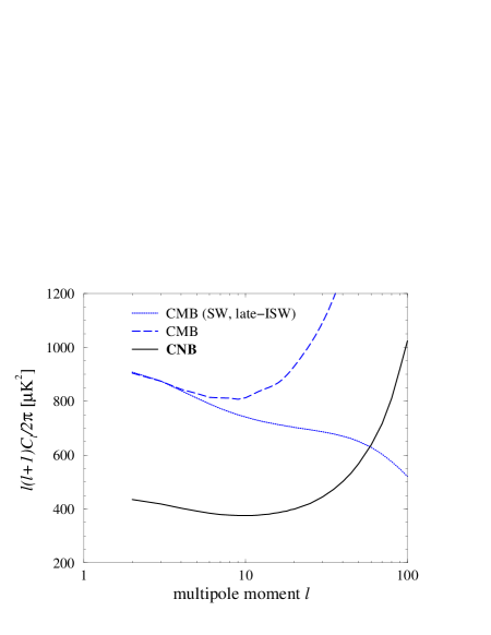
Figure 1: The temperature anisotropy power spectrum for a species of relativistic neutrinos is shown for multipole moments $\ell<100$. The sources of anisotropy are SW and ISW effects, including intrinsic perturbations of the neutrino spectrum at decoupling, which occured at $z\sim 10^{10}$. For comparison, we also show the SW and late-ISW contributions to the CMB anisotropy spectrum calculated following the same method. The amplitude is set by using $A_{WMAP}=0.9$ Spergel:2006hy ; CMBfast . We also show the full CMB power spectrum calculated using CMBfast Seljak:1996is .

We now present the results of detailed calculations of the CNB temperature anisotropy spectrum. We assume relativistic neutrinos, so that the temperature fluctuations are given by

$$\Delta_{0}(\hat{n}) = \frac{1}{2}\phi(\tau_{dec},(\tau_{0}-\tau_{dec})\hat{n})$$ (14)

$$+ 2\int^{\tau_{0}-\tau_{dec}}_{0}d\lambda\,\phi_{,\tau}(\tau_{0}-\lambda,\lambda\hat{n}).$$ (15)

We assume a primordial spectrum of scale-invariant density perturbations, where the Fourier modes of the gravitational potential obey $\langle\phi(\vec{k})\phi(\vec{k}^{\prime})\rangle=4\pi k^{3}P_{\phi}(k)\delta(\vec{k}+\vec{k}^{\prime})$, with a power spectrum $P_{\phi}(k)=Ak^{n_{s}-4}$. For the power-law index, $n_{s}=1$. The background cosmology is modeled as a spatially-flat FRW spacetime filled by a three-component fluid, consisting of radiation, matter, and cosmological constant. The Hubble constant evolves as

$$H(a)=H_{0}\sqrt{\Omega_{m}({a_{0}}/{a})^{3}+\Omega_{r}({a_{0}}/{a})^{4}+\Omega_{\Lambda}}$$ (16)

where we use $H_{0}=100\,h$ km/s/Mpc, $h=0.7$, $\Omega_{m}=0.3$, $\Omega_{r}=4.2\times 10^{-5}/h^{2}$, and $\Omega_{\Lambda}=1-\Omega_{m}-\Omega_{r}$. The evolution of the gravitational potential due to adiabatic density perturbations is determined by Mukhanov ; Ma:1995ey

$$\ddot{\phi}+3{\cal H}(1+c_{s}^{2})\dot{\phi}+\left(2\dot{\cal H}+(1+3c_{s}^{2}){\cal H}^{2}+c_{s}^{2}k^{2}\right)\phi=0$$ (17)

where the dot indicates the derivative with respect to conformal time, ${\cal H}=\dot{a}/a=aH$, and the adiabatic sound speed is $c_{s}^{2}=\frac{1}{3}/(1+\frac{3}{4}\frac{\rho_{m}}{\rho_{r}})$. Initial conditions are chosen so that $\phi=1,\,\dot{\phi}=0$ deep in the radiation era. Last scattering occurs sharply at $z=10^{10}$ for the CNB ($1100$ for the CMB). Finally, the $C_{\ell}$’s are obtained by evaluating

$$C_{\ell}=(4\pi)^{2}A\,\int d\ln k\,\left(\frac{1}{2}\phi(\tau_{dec},k)j_{\ell}(k(\tau_{0}-\tau_{dec}))+2\int_{0}^{\tau_{0}-\tau_{dec}}d\lambda\,\phi_{,\tau}(\tau_{0}-\lambda,\lambda)j_{\ell}(k\lambda)\right)^{2}.$$ (18)

To normalize to WMAP, we set the constant $A=200\pi A_{WMAP}({T_{\nu}}/{T_{CMB}})^{2}\mu K^{2}$. The resulting multipole spectrum is shown in Figure 1, our main result. It is interesting to note that, whereas the CNB SW effect is much stronger than for the CMB, a strong, negative cross-correlation between the early-ISW and the SW effects greatly reduces the overall anisotropy power spectrum on large angular scales. We limit our power spectrum to $\ell<100$; on smaller angular scales we expect the effects of bulk anisotropic pressure or shear, which we have ignored, to be important. For comparison, we also show the SW and late-ISW contributions to the CMB, as well as the full CMB. These results are consistent with the earlier results of Hu et al. Hu:1995fq , where the CNB anisotropy in a SCDM universe was considered. Overall, the rms temperature fluctuations in the CNB are smaller than for the CMB.

The anisotropy power spectrum for non-relativisitic neutrinos is shown in Figure 2. Since the spectrum depends on the momentum of the neutrinos, we focus on values of momentum $q\sim T_{\nu}$ for comparison with anisotropies at the peak of the relativistic neutrino flux spectrum. We see that the overall amplitude is comparable to the relativistic result at the lowest multipoles, as seen in Figure 2, but is much smaller otherwise, due to the suppression of the SW contribution from decoupling. The dominant effect is due to the $\Gamma_{,\lambda}\phi$ term in the line-of-sight integration in equation (9), whereas the $\phi_{,\tau}$ term contributes a much smaller fraction than in the relativistic case. In the limit $q\gg m_{\nu}>T_{\nu}$ the relativistic result is obtained. Although low energy neutrino capture by galaxies is an anisotropic effect which removes the slowest-moving particles from the power spectrum, the mass estimates used and the currently favored upper bounds predict a negligible amount of gravitational clustering.

Figure 2: The temperature anisotropy power spectrum for a species of non-relativistic (NR) neutrinos is shown. We use neutrino mass $m_{\nu}=0.05$ eV and momentum $q=T_{\nu}$. The results do not change appreciably for $0.1\leq q/T\leq 10$. The SW effect is strongly suppressed, and only a line-of-sight term contributes to the anisotropy. For comparison, we also show the relativistic (R) CNB anisotropy spectrum.

Our analysis thus far treats the primordial neutrinos analogously to CMB photons. However, there are several important ways in which neutrinos differ from photons: exclusive interaction via the weak force, spin-statistics, mass, and flavor oscillation. The first factor has been taken into account in determining the neutrino decoupling time, and ignoring important CMB phenomena such as reionization. Even in the early universe, when conditions were extremely hot and dense, neutrino scattering was negligibly rare. Present day interactions with interstellar matter are far less significant in comparison with electromagnetic processes. The CNB should also differ from the CMB in the absence of an acoustic peak. The second factor means that neutrinos obey Fermi-Dirac statistics. The primordial, relativistic neutrinos have a thermal, blackbody spectrum, but very low momentum neutrinos could be degenerate, a possibility which we will not explore DegenerateNeutrinos . The third factor is significant, as only one of the neutrino mass states may be relativistic today. This also leads to the fourth, final factor: flavor oscillation. The neutrino flavor states $\nu_{j}$, $j=\{e,\,\mu,\,\tau\}$ are a superposition of mass eigenstates, $\nu_{i}$, $i=\{1,\,2,\,3\}$. Hence, the flavor of an individual neutrino oscillates with time.

The CNB neutrinos have travelled over $\sim 45$ Gpc from the time of decoupling to the present. Very early on, the universe was dense enough to be characterized as electron-flavored matter, a distinction which determined the type of matter oscillations. However the vast majority of the subsequent travel by neutrinos has occurred in vacuum, where the path-length for neutrino mixing is very short. We can use the two-flavor mixing model as an approximation, whereby the mixing probability is

$$P(\nu_{i}\to\nu_{j})=\sin^{2}2\theta_{ij}\sin^{2}\left(\frac{\Delta m_{ij}^{2}L}{4E_{\nu}}\right)$$ (19)

Using $E_{\nu}\sim T_{\nu}$ we find a microscopic oscillation length. Hence, the CNB should be well mixed Khlopov1981 , with flavor abundances dictated by the mixing angles $\theta_{ij}$. This means the spectrum of primordial $\nu_{e}$’s should be a mixture of relativistic $\nu_{1}$’s and nonrelativistic $\nu_{2,3}$’s. Similarly, the anisotropy spectrum should be a mixture.

The anisotropy power spectrum for the $e,\,\mu,\,\tau$-neutrinos will be a mixture of the spectra for the relativistic and nonrelativistic neutrino mass eigenstates. Since the anisotropy for the relativistic species rapidly dominates with increasing multipole moment, we can ignore the nonrelativistic contributions to leading order. Also, sufficiently low-momentum, nonrelativistic neutrinos will get gravitationally captured in galaxies and clusters. Since we are assuming an inverted neutrino mass spectrum, the lightest neutrino is $\nu_{1}$. We refer to the lepton mass mixing matrix to determine what fraction $\nu_{1}$ contributes to the flavor eigenstates, and to the temperature anisotropy in a particular flavor. For $\nu_{e}$, this matrix element is $c_{12}c_{13}$ where $c_{ij}\equiv\cos\theta_{ij}$, so the temperature anisotropy of electron neutrinos is $\Delta T(\nu_{e})=c_{12}c_{13}\Delta T(\nu_{1})$. The power spectrum is quadratic in this fraction, $C_{l}(\nu_{e})=(c_{12}c_{13})^{2}C_{l}(\nu_{1})$. Using currently accepted values of the mixing angles, $\theta_{12}\approx 34^{\circ}$ and $c_{13}\approx 1$ Kayser , then the electron neutrino temperature anisotropy power spectrum is approximately $70\%$ of the relativistic CNB amplitude given in Figure 1.

Thus, we have determined the large-angle CNB temperature anisotropy. It is important to note that there is an extensive literature on cosmological neutrinos (e.g. Lesgourgues:2006nd ) including their effect on the CMB. In fact,the existence of the CNB Dicke1965 ; Gerstein1966 was immediately anticipated following the discovery of the CMB by Penzias and Wilson Penzias1965 . Predictions of neutrino number density anisotropies have been attempted, with an eye toward their effect on the CMB power spectrum Trotta , however there are too many free parameters for such work to be conclusive. Instead, our approach in analogizing microwave background temperature variations to the neutrino background seems to have been largely avoided, but there is no reason we should expect primordial neutrinos not to undergo SW and ISW effects. The one notable exception is Ref. Hu:1995fq in which the full Boltzmann equations for the neutrino brightness perturbation is evolved in a cold dark matter dominated universe with $\Omega_{m}=1$. Although this is a standard by-product of CMB calculations, their Figure 12 is the only other display of the CNB anisotropy power spectrum of which we are aware.

It would be surprising if there are foreground neutrino sources which contaminate the CNB. Although there exists a rich background of astrophysical, atmospherical, and terrestrial neutrino sources, it is hard to believe that the spectrum extends down to $1.9$ K, considering that the exclusive weak-force interaction would prevent any process but redshifting from reducing conventional neutrino energies by that many orders of magnitude.

We also note that none of the current proposals for CNB detection would be capable of observing the angularly dependent anisotropy behavior described in this paper. Of all prospects for measurement, annihilation with UHE neutrinos due to a resonance with Z bosons would likely give the most unequivocal proof for the existence the CNB Gelmini:2004hg . In this scenario, a burst of cosmic rays from a topological defect is anomalously absorbed by the CNB, causing observers of the UHE$\nu$’s to see dips at characteristic energies corresponding to the three masses of the CNB neutrinos. However the discovery of a topological defect required to produce the cosmic rays would be so astounding in its own right that this method does not currently seem promising.

We expect the CNB anisotropy is nearly impossible to detect directly. First, the cross section for a relic neutrino to scatter off a nucleus is tremendously low. Estimating $\sigma\approx G_{F}^{2}E_{\nu}^{2}\simeq 4\times 10^{-64}{\rm cm}^{2}$, this makes dark matter detection look easy. Second, a threshold energy $E_{\nu}\sim 10^{-4}$ eV, many orders of magnitude below the detection sensitivity of current experiments, would be needed to see the peak of the CNB spectrum; more still to see the minute anisotropic temperature variations. Third, the large volume of material necessary to build a suitable detector makes for poor angular resolution. Nonetheless, the anisotropic CNB is there.

The hurdles in even observing the CNB are so significant that to speculate as to its angular appearance must seem somewhat presumptuous. We make no assertions about the feasibility of such a prospect beyond noting that many of the accomplishments in neutrino physics experimentation were completely unanticipated or considered unattainable until shortly before their implementation. We recall Wolfgang Pauli’s remark shortly after conceiving of the neutrino in 1930 Hoyle : “I’ve done a terrible thing today, something which no theoretical physicist should ever do. I have suggested something that can never be verified experimentally.” Hopefully, a discussion of CNB properties will someday cease to seem as exclusively theoretical as it does today, just as the neutrino itself once did to Pauli.

- (1) E. W. Kolb and M. S. Turner, The Early Universe, Addison-Wesley (1990).
- (2) S. Hannestad, arXiv:hep-ph/0602058.
- (3) B. Kayser, “Neutrino Mass, Mixing, and Flavor Change,” in The Particle Data Group (S. Eidelman et al.), Phys. Lett. B592, 1 (2004).
- (4) S. Fukuda et al., [Super-Kamiokande Collaboration], Phys. Lett. B539, 179 (2002).
- (5) Q. R. Ahmad et al., [SNO Collaboration], Phys. Rev. Lett. 89, 011301 (2002); ibid., 011302 (2002).
- (6) K. Eguchi et al., [KamLAND Collaboration], Phys. Rev. Lett. 90, 021802 (2003).
- (7) C. P. Ma and E. Bertschinger, Astrophys. J. 455, 7 (1995).
- (8) R. K. Sachs, A. M. Wolfe, Astrophys. J. 147, 73 (1967).
- (9) M. J. Rees, D. W. Sciama, Nat. 217, 511 (1968).
- (10) V. F. Mukhanov, H. A. Feldman and R. H. Brandenberger, Phys. Rept. 215, 203 (1992).
- (11) D. N. Spergel et al., “Wilkinson Microwave Anisotropy Probe (WMAP) three year results: arXiv:astro-ph/0603449.
- (12) See CMBfast (www.cmbfast.org) documentation for an explanation of the WMAP normalization.
- (13) U. Seljak and M. Zaldarriaga, Astrophys. J. 469, 437 (1996).
- (14) W. Hu, D. Scott, N. Sugiyama and M. J. White, Phys. Rev. D 52, 5498 (1995).
- (15) K. Ichikawa and M. Kawasaki, Phys. Rev. D 67, 063510 (2003).
- (16) Ya. B. Zeldovich and M. Khlopov, Sov. Phys. Usp. 24, 755 (1981).
- (17) J. Lesgourgues and S. Pastor, Phys. Rept. 429, 307 (2006).
- (18) R. H. Dicke, P. J. E. Peebles, P. G. Roll, and D. T. Wilkinson, Astrophys. J. 142, 414 (1965).
- (19) S. S. Gerstein and Ya. B. Zeldovich, Sov. Phys. JETP Lett. 4, 120 (1966).
- (20) A. A. Penzias and R. W. Wilson, Astrophys. J. 142, 419 (1965).
- (21) R. Trotta and A. Melchiorri, Phys. Rev. Lett. 95, 011305 (2005).
- (22) G. B. Gelmini, Phys. Scripta T121, 131 (2005).
- (23) F. Hoyle, Proc. Roy. Soc. London A 301, 171 (1967).