Spitzer SAGE survey of the Large Magellanic Cloud II: Evolved Stars and Infrared Color Magnitude Diagrams

Abstract

Color–magnitude diagrams (CMDs) are presented for the Spitzer SAGE (Surveying the Agents of a Galaxy’s Evolution) survey of the Large Magellanic Cloud (LMC). IRAC and MIPS 24 $\mu$m epoch one data are presented. These data represent the deepest, widest mid–infrared CMDs of their kind ever produced in the LMC. Combined with the 2MASS survey, the diagrams are used to delineate the evolved stellar populations in the Large Magellanic Cloud as well as Galactic foreground and extragalactic background populations. Some 32000 evolved stars brighter than the tip of the red giant branch are identified. Of these, approximately 17500 are classified as oxygen–rich, 7000 carbon–rich, and another 1200 as “extreme” asymptotic giant branch (AGB) stars. Brighter members of the latter group have been called “obscured” AGB stars in the literature owing to their dusty circumstellar envelopes. A large number (1200) of luminous oxygen–rich AGB stars/M supergiants are also identified. Finally, there is strong evidence from the 24 $\mu$m MIPS channel that previously unexplored, lower luminosity oxygen–rich AGB stars contribute significantly to the mass loss budget of the LMC (1200 such sources are identified).

1 Introduction

The Spitzer Space Telescope (Spitzer), with its rapid wide field mapping capability and sensitivity, allows us to survey the thermal emission produced by mass loss from individual evolved stars in the nearest galaxies. Meixner et al. (2006) presented the Spitzer SAGE (Surveying the Agents of a Galaxy’s Evolution) survey of the Large Magellanic Cloud (LMC) along with a detailed description of its goals, expected extent in depth and coverage and some preliminary results. The SAGE survey is designed to enable studies of the life–cycle of baryonic matter, as traced by dust emission, in the LMC. In this work, we focus on one corner stone of this life–cycle, the dusty evolved star population, which is returning matter to the interstellar medium. Coupled with detailed star formation history (SFH) studies at optical wavelengths, SAGE provides the opportunity to link specific LMC populations to their dust content as a function of key parameters such as metallicity and age. Such analyses can, in turn, be used to validate predictive models of infrared emission in high redshift galaxies. In the present paper, we focus on the necessary first step of identification and characterization of the dusty evolved star populations.

SAGE provides a global view of the dust producing stellar populations in the LMC that will contribute to our understanding of evolved stars. Essentially all significant, dusty, mass-losing stars in the LMC will be detected by SAGE as it provides the deepest, widest survey in the near– and mid-infrared wavelengths (3–24 microns) produced to date for this nearby galaxy. These wavelengths are particularly well suited to the investigation of the late stages of stellar evolution because once beyond the near–infrared (five microns), emission from circumstellar dust can become the dominant source of emission over the radiation from the photosphere. By eight microns, many LMC sources show appreciable emission from dust, and the MIPS 24 micron band is extremely sensitive to cool envelopes with excess dust emission even for sources with little evidence of strong dust excess at shorter wavelengths.

SAGE builds on and leverages a wealth of past observations of evolved stars in the LMC. Optical (MCPS; see Zaritsky et al., 2004, and http://ngala.as.arizona.edu/dennis/mcsurvey.html) and near–infrared surveys, for example, DENIS (Epchtein et al., 1994) and 2MASS (Skrutskie et al., 2006), have provided a global view of the LMC at shorter wavelengths. See Cioni et al. (2006) and Nikolaev & Weinberg (2000) for LMC data from these two surveys, respectively. The Infrared Astronomy Satellite (IRAS, Neugebauer et al., 1984) revolutionized the study of evolved stars by observing objects with luminous dusty envelopes at long wavelengths. This survey has provided samples of stars in the LMC to be observed in greater detail up to the present, including spectroscopic observations with Spitzer; see Zijlstra et al. (2006) and Markwick–Kemper et al. (2005). However, IRAS was only sensitive enough to observe the brightest sources in the LMC (Schwering, 1989) from which several hundreds of mass–losing evolved star candidates could be identified (Loup et al., 1997). The successful Midcourse Space Experiment (MSX, Price et al., 2001) was about four times more sensitive and provided a full LMC survey (Egan et al., 2001). SAGE should be roughly 1000 times more sensitive than MSX when complete (Meixner et al., 2006, the present data are roughly 400 times more sensitive). While near–infrared and optical surveys of the LMC have identified lower mass evolved stars, only SAGE has the depth to detect such stars at wavelengths necessary to explicitly explore their dust properties. The ISOCAM Magellanic Cloud Mini–Survey (see Cioni et al., 2003) has provided a preliminary mid–infrared view of the LMC over a small field of view (0.3 square degrees) near the depth of SAGE.

The SAGE sensitivity and areal coverage of the entire LMC will allow a detailed quantitative derivation of the global mass loss budget from all stellar populations when combined with existing and future mid–infrared spectroscopic observations of the asymptotic giant branch (AGB) stars and supergiants; for example, see van Loon et al. (1999), van Loon et al. (2005), Markwick–Kemper et al. (2005), and Zijlstra et al. (2006). Several studies have derived detailed SFHs in the LMC from a variety of field locations and clusters (Holtzman et al., 1999; Olsen, 1999) using principally optical color–magnitude diagrams (CMDs) and sophisticated stellar models and fitting techniques (e.g. Harris & Zaritsky, 2001). Recently, Cioni et al. (2006) made a global SFH calculation using the 2MASS and DENIS surveys. Their new models still have difficulties producing the correct mix of observed carbon–rich AGB stars (C–rich or C–stars) versus oxygen–rich AGB stars (O–rich or M stars), but their extension to these wavelengths of the general technique is a great advance. With SAGE, we will be able to associate the mass–loss and chemical properties of the AGB stars in the LMC with their known evolutionary state from existing SFH studies. This coupling can then be used to investigate, with precision, the evolutionary status of galaxies which lie at much larger distances through the development and testing of detailed population synthesis models (for example, see Mouhcine & Lançon, 2003).

In this paper, we continue the analysis begun by Meixner et al. (2006) by presenting CMDs of the survey data for the first of two epochs. We lay the ground work for the detailed analysis to come when the full SAGE survey is available by dissecting the observed CMDs and indicating where various LMC and fore and background populations reside in these diagrams. The present paper covers approximately 49 square degrees in the IRAC bands and MIPS 24 $\mu$m band.

2 The SAGE Catalog and Epoch One Source List

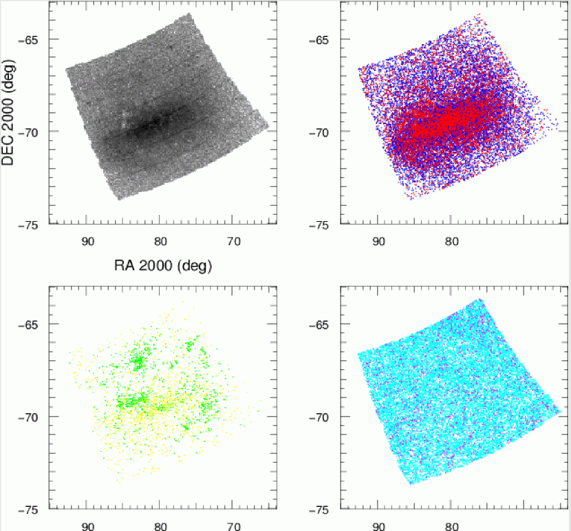
Figure 1: Positions of IRAC sources for the epoch one dataset covering approximately 49 square degrees centered on the Large Magellanic Cloud. The upper left panel shows the source density in gray scale, highlighting the stellar bar. The figure shows sources detected at $J$, [3.6], and [8.0]. The points are color coded according to stellar or object type (see text and Figure 3 for details). The upper right panel shows the distribution of carbon–rich (red) and oxygen–rich (blue) stars. The lower left panel shows the “extreme” asymptotic giant branch stars (yellow) and luminous oxygen–rich stars and M supergiants (green). The lower right panel shows two source types which may be dominated by background galaxies: the spatial distributions are uniform (see text). The magenta points in this panel show objects with strong $J-$[8.0] excess while the cyan objects have no $J-$band counterparts.

The SAGE epoch one catalog is discussed by Meixner et al. (2006). The present source list contains the first epoch data for the IRAC (3.6 $\mu$m, 4.5 $\mu$m, 5.8 $\mu$m, and 8.0 $\mu$m) bands processed by the IRAC pipeline as of May 04, 2006. This amounts to a coverage of approximately 49 square degrees (Figure 1). The current IRAC source list includes a merged source list with the 2MASS point source catalog. Details of the SAGE IRAC pipeline processing are given by Meixner et al. (2006); the pipeline is based on the GLIMPSE pipeline (Benjamin et al., 2003). Briefly, the IRAC data were taken such that a typical point on the sky was observed twice within a $\sim$ one degree square “tile.” The frames are analyzed with a custom DAOPHOT (Stetson, 1987) package developed by the GLIMPSE team. The catalog photometry is based upon combining the individual frame photometry (i.e., photometry is not done on the mosaic tiles). Each tile itself overlaps at the edges with adjacent tiles and the comparison of source photometry between tiles results in more detections in the overlap regions. The IRAC bands and 2MASS catalog photometry are merged in the so–called “cross–band” merge step of the pipeline which is based upon positional matching (see Meixner et al., 2006, and references therein for details) of the final flux calibrated sources in each IRAC and 2MASS band. Systematic offsets in the IRAC–2MASS merging are less than 0.3^′′.

The combined IRAC–2MASS source list analyzed in this paper contains approximately four million sources with a 3.6 $\mu$m data point (the deepest IRAC band in terms of SAGE photometry). There are approximately 820000 sources with $J$ and [3.6] magnitudes of which nearly 650000 have errors less than 0.1 mag in each of $J$ and [3.6]. An additional 10000 sources have individual $J$ and [3.6] errors less than 0.2 mag and the remainder have errors of less than 0.3 mag. The present dataset further has 250000 8 $\mu$m sources which also have 3.6 $\mu$m data (90$\%$ have [8.0] and [3.6] photometry with errors less than 0.1 mag). The analogous numbers for $J$ and 8 $\mu$m are 230000 and 91$\%$. The IRAC uncertainties are those reported by the custom DAOPHOT package used in the pipeline and so include photon statistics and fitting uncertainties. The 2MASS errors are taken from the 2MASS point source catalog. The initial frames delivered from the Spitzer Science Center (SSC) are flux calibrated (SSC pipeline version s12.0). A network of 238 absolute calibration stars has been developed near the area observed by SAGE (137 stars overlap the SAGE survey area) using the identical technique by which IRAC primary standards were established (Cohen et al., 2003). Comparison between predicted and observed magnitudes for stars in this network indicate that ensemble systematic uncertainties in any IRAC band do not exceed the five percent level.

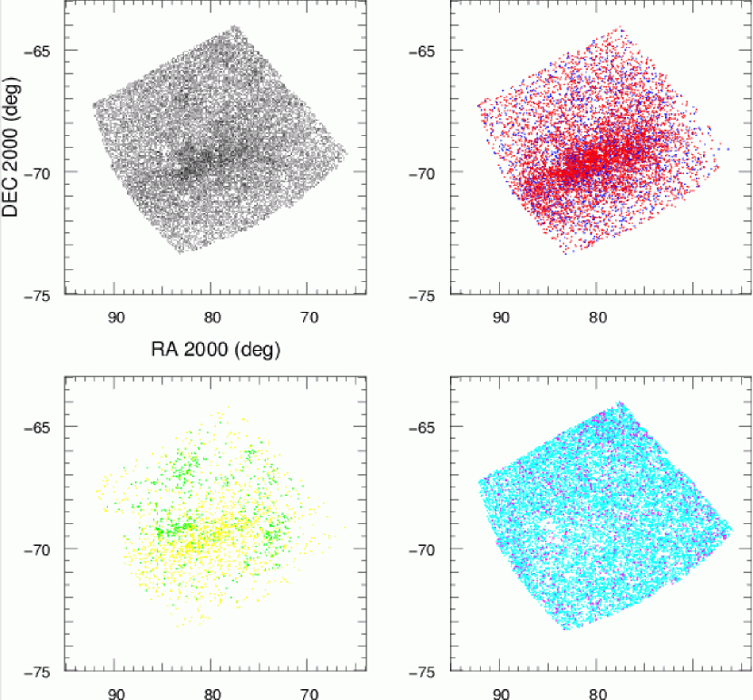
Figure 2: Same as Figure 1, but for sources detected at 24 $\mu$m and matched to IRAC counterparts.

The present source list for the MIPS 24 $\mu$m band covers a similar area as for the IRAC source list (Figure 2). The 24 $\mu$m source list (64800 sources) is for epoch one data processed as of May, 19 2006. Details of the MIPS processing are given by Gordon et al. (2005) and Meixner et al. (2006). The MIPS data were observed in sets of scans with each set covering a four degree by 25 arcminute strip. The photometry was extracted via PSF fitting using the StarFinder program (Diolaiti et al., 2000).

The IRAC and MIPS data presented here were merged after assembly of the individual catalogs by the respective pipeline teams. The IRAC sources (those with valid 8 $\mu$m magnitudes) were matched within 1^′′ of the MIPS 24 $\mu$m sources, choosing the closest companion if multiple possibilities existed. This resulted in 27741 matches with a an average difference in position of 0.42^′′ (and systematic offsets in RA of $-$0.024^′′ and DEC of $-$0.004^′′) and a distribution of offsets with one sigma standard deviation of approximately 0.25^′′. The 24 $\mu$m pixel size is 2.6^′′ and the diffraction limited $\lambda$/D is approximately 6^′′. Crowding induced errors in the IRAC photometry and the matching of sources between IRAC and MIPS are discussed in appendix A below.

About 42$\%$ of the MIPS sources have IRAC matches. What about the other 58$\%$? This number of non–matches suggests a large number of very red sources toward the LMC. As the analysis below will suggest, some of these may be background galaxies not detected by IRAC. Others could be embedded sources in the LMC, and many could be slightly extended sources which have no point–like IRAC counterpart. Detailed analysis of the 24 $\mu$m and other MIPS channels will be the subject of a subsequent SAGE paper.

3 Color–Magnitude Diagrams

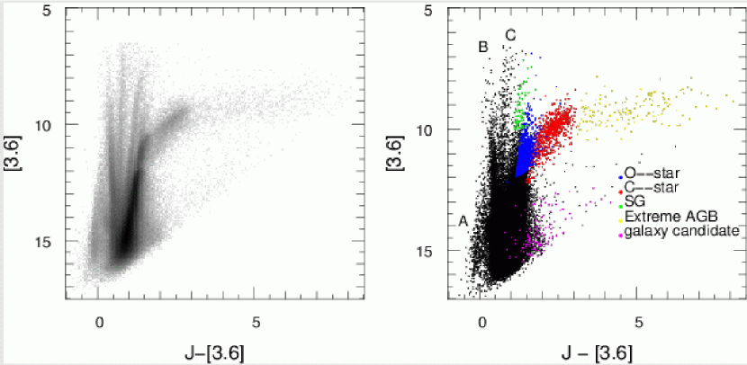
Figure 3: $J-$[3.6] $vs.$ [3.6] color–magnitude diagram (CMD, right panel) and associated Hess diagram (left panel). The tip of the red giant branch is located at [3.6] $=$ 11.85 mag. The color coding is as follows. All points in the source list are shown as black dots. Blue dots are oxygen–rich asymptotic giant branch (AGB) stars, and red dots are carbon–rich AGB stars. The yellow dots represent “extreme” AGB stars while the green dots are M supergiants and luminous oxygen–rich stars. The magenta dots may be predominantly background galaxies (see text). In the Hess diagram, the red giant branch is the most densely populated region. The peak density is approximately 2400 stars in a 0.045$\times$0.055 square magnitude pixel and occurs at $J-$[3.6], [3.6] $=$ 0.8, 15.6. The prominent sequences are described in the text; see also Table 1. The features labeled as A, B, and C correspond to the same features seen in the 2MASS CMD (Nikolaev & Weinberg, 2000). For clarity, only every 10th source is plotted in the CMD (all points are plotted in the Hess diagram).

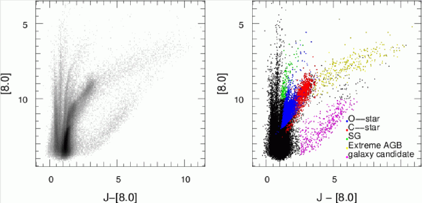
Figure 4: Same as Figure 3, but for the $J-$[8.0] $vs.$ [8.0] color–magnitude diagram and corresponding Hess diagram. For clarity, only every 5th source is plotted in the CMD.

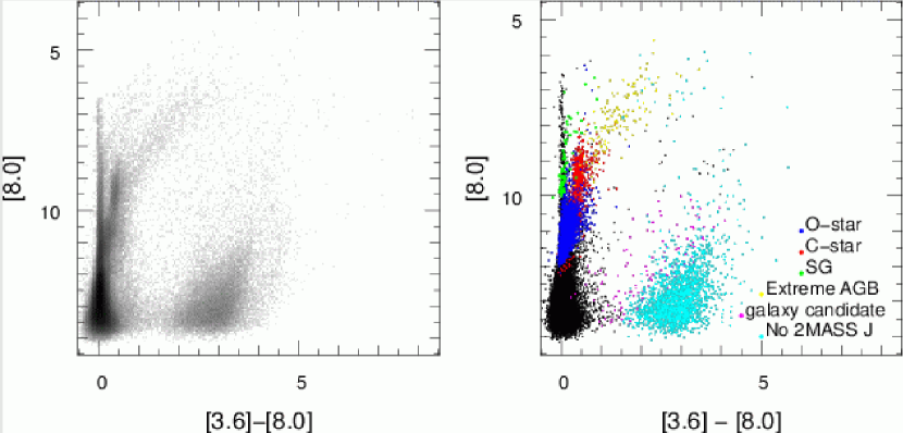
Figure 5: Same as Figure 3, but for the [3.6]$-$[8.0] $vs.$ [8.0] color–magnitude diagram and Hess diagram. Additionally, the cyan points may be dominated by background galaxies, but which have no 2MASS $J-$band detection. The brightest cyan points ([3.6] $\mathrel{\hbox{\hbox to0.0pt{\hbox{\lower 4.0pt\hbox{$\sim$}}\hss}\hbox{$<$}}}$10 mag) are probably mostly luminous LMC sources; see text. For clarity, only every 10th source is plotted in the CMD.

Figures 3–6 present four Hess diagrams (Hess diagrams are a two dimensional histogram of the CMD which give the number of stars per unit magnitude and color with the grayscale representations graphically showing the relative source densities) and their corresponding CMDs produced with IRAC, MIPS, and 2MASS photometry. The Hess diagrams are binned into 200$\times$200 pixels (i.e., bins of color and magnitude).

There is a wealth of information in these diagrams. Egan et al. (2001) presented near–infrared$+$mid–infrared CMDs for the entire LMC from the MSX satellite and 2MASS (Skrutskie et al., 2006). The MSX sensitivity is approximately eight magnitudes brighter than SAGE, so that the present survey will greatly extend the mid–infrared view of the LMC begun by IRAS and MSX.

In the following, all near–infrared photometry has been taken from the 2MASS point source catalog (Skrutskie et al., 2006). These data have been merged with the SAGE photometry using the SAGE IRAC pipeline (see above). The diagrams in this paper use IRAC and MIPS photometry converted to magnitudes using the following zero points (Reach et al., 2005; Engelbracht et al., 2006): [3.6] zero mag $=$ 280.9 Jy, $\lambda_{\circ}$ $=$ 3.55 $\mu$m; [8.0] zero mag $=$ 64.13 Jy, $\lambda_{\circ}$ $=$ 7.872 $\mu$m, [24] zero mag $=$ 7.15 Jy, $\lambda_{\circ}$ $=$ 23.68 $\mu$m.

3.1 IRAC and 2MASS Color–Magnitude Diagrams

Earlier “all–LMC” surveys by IRAS and MSX had sensitivities 1000 times less than SAGE. While these surveys could detect the brightest sources in the LMC, it has been more difficult to put them in the overall context of the entire stellar population. In the following sections we analize the SAGE CMDs with an emphasis on identifying the main evolved star populations and enumerating their relative contributions to the total source counts. This basic accounting will help guide future detailed studies using the SAGE data base as well as provide a comprehensive means for selecting follow–up targets for spectroscopic study.

3.1.1 $J-$[3.6] vs. [3.6]

The 3.6 $\mu$m channel is by far the most sensitive of the IRAC bands and as such provides the deepest photometry to compare to 2MASS. Nikolaev & Weinberg (2000) presented the 2MASS CMD for the LMC. Comparison of their Figure 3 with the $J-$[3.6] $vs.$ [3.6] diagram shown in Figure 3 shows the same sequences with perhaps slightly more “contrast” in the features owing to the longer baseline in wavelength. Starting with $J-$[3.6] $vs.$ [3.6], the first prominent finger ($J-$[3.6] $\mathrel{\hbox{\hbox to0.0pt{\hbox{\lower 4.0pt\hbox{$\sim$}}\hss}\hbox{$<$}}}$0.5) reaching to bright magnitudes ([3.6]$\sim$6) corresponds to region “B” of Nikolaev & Weinberg (2000), young A–G supergiants. There is clearly a slope to this finger indicating predominantly an LMC population (foreground sequences appear vertical due to the varying distance of the sources which smears out their magnitudes but not their colors). The brightest objects in this sequence include Galactic K and G dwarfs. To the blue and fainter of this feature lies the OB star locus in the LMC (region “A” of Nikolaev & Weinberg, 2000).

The next sequence to the red is the vertical one reaching to bright magnitudes. This finger consists mainly of foreground dwarfs and giants (region “C” of Nikolaev & Weinberg, 2000). In fact, Nikolaev & Weinberg (2000) find $\mathrel{\hbox{\hbox to0.0pt{\hbox{\lower 4.0pt\hbox{$\sim$}}\hss}\hbox{$>$}}}$70$\%$ of the stars in this region of the diagram are Galactic foreground. The importance of this contamination declines at lower brightnesses relative to the rest of the diagram as is clearly seen in the Hess diagram. Simple models of Galactic structure (for example, Blum et al., 1995) predict only several late M stars in the LMC foreground owing to their rarity. The remaining sequences in the $J-$[3.6] $vs.$ [3.6] diagram are predominantly LMC red giant branch stars (RGB), AGB stars and late–type (mostly M) supergiants (SG).

Cioni et al. (2006) computed star formation history models of the LMC using the 2MASS CMD and new stellar models (Marigo et al., 2003). The Marigo et al. (2003) models could, for the first time, reach the observed red colors of the C–stars and thus explain the origin of their location in the CMD. Based on their analysis of the 2MASS CMD, Cioni et al. (2006) divided the region above the tip of the RGB (TRGB) into O–rich and C–rich zones using relations for the 2MASS $J-K$ color and $K$ magnitude. In Figures 3–6 the blue and red points correspond to Cioni et al.’s photometric division of O–rich and C–rich stars, respectively, using 2MASS colors (their equations 5–7). The C–star and O–rich star loci are well defined and separated in our CMDs, lending support to the Cioni et al. (2006) criterion.

The green points in Figure 3 (and following figures) represent M SG and luminous, O–rich M stars. The locus was obtained by using a cut in the $J-K$ $vs.$ $K$ plane which paralleled the Cioni et al. (2006) relation for O–rich AGB stars, but was displaced to the blue enough to encompass the obvious sequence in Figure 3 (left panel) for the $J-$[3.6] $vs.$ [3.6] diagram. Cross reference with SIMBAD (here and elsewhere in this work, SIMBAD searches are associated with a 5^′′ search radius) shows that several of the Elias, Frogel, & Humphreys (1985) supergiants fall on this sequence as well as luminous M stars identified by Massey (2002). Nikolaev & Weinberg (2000) confirm the presence of known M SG on the associated $J-K$ sequence. These luminous, late–type stars are young and thus trace regions in the LMC of recent star formation (M SG have ages of about 10 Myr while the most luminous AGB stars are a few hundreds of Myr). This is seen in Figures 1 and 2; contrast the clumpy and non–uniform distribution of the young stars with the more smooth distribution of the older C–stars and O–stars. The distribution of young M supergiants qualitatively matches the structure seen in other tracers of star formation in the LMC; see, for example, the H_α map of Gaustad et al. (2001) and the UV map of Smith et al. (1987). These and other tracers are conveniently summarized in Figure 1 of Meixner et al. (2006).

The yellow points in Figure 3 represent a group of objects which show the effects of dusty circumstellar envelopes. These “extreme” AGB stars are discussed in the next section where their $J-$[8.0] color is used to define their selection. Likewise, a sequence which may be dominated by background galaxies is given by the magenta points in Figure 3. These sources are defined by their $J-$[8.0] color also (see below), and shown in the $J-$[3.6] $vs.$ [3.6] CMD to demonstrate how their excess color is dominated by longer wavelength emission.

3.1.2 $J-$[8.0] $vs.$ [8.0]

C–stars have $J-$[3.6] color which extend up to about 3.0 ($J-K$ $\mathrel{\hbox{\hbox to0.0pt{\hbox{\lower 4.0pt\hbox{$\sim$}}\hss}\hbox{$<$}}}$2.1); at this point, the sequence continues at nearly constant [3.6] brightness (see Figure 3) to very red colors (whereas the $K$ magnitudes break sharply to fainter brightnesses here). In the $J-$[8.0] $vs.$ [8.0] CMD shown in Figure 4, the analogous break occurs at $J-$[8.0] $\approx$ 3.5 with the [8.0] data points trending to brighter magnitudes, but with different slope than before. We have drawn this “break” in the apparent C–star relation arbitrarily at $J-$[3.6] $=$ 3.1 and coded the redder objects with [3.6] $\geq$ 10.5 as yellow points in Figures 3–6. We call these stars “extreme” AGB stars. The brightest members of this sequence (IRAS sources) and the red stars above it have been the subject of numerous earlier studies to search for and characterize obscured AGB stars. See, for example, Loup et al. (1997); van Loon et al. (1999). While most of the objects in this sequence are C–stars, not all of them are (see, for example, Zijlstra et al., 2006); spectroscopic confirmation is required to confidently place any particular source in the C–star or M–star category. A number of investigators have also studied representatives of the “extreme” star sequence in detail at shorter wavelengths. Hughes & Wood (1990) investigated the AGB stars which span the “visible” C–star locus and bluest part of the present “extreme” star locus ($J-$[8.0] $\mathrel{\hbox{\hbox to0.0pt{\hbox{\lower 4.0pt\hbox{$\sim$}}\hss}\hbox{$<$}}}$4).

The separation of the stellar sequences becomes more apparent in the $J-$[8.0] $vs.$ [8.0] diagram. The prominent middle vertical sequence (“C”) now breaks into two clear sequences with foreground late K giants further to the red than earlier G type giants.

An obvious sequence of sources becomes evident in the $J-$[8.0] $vs.$ [8.0] diagram. These points are color coded in magenta. As pointed out by Meixner et al. (2006), comparison of the [8.0] number counts to those for deep extragalactic fields (Fazio et al., 2004) indicates these are predominantly background galaxies. The same sources are shown in the $J-$[3.6] diagram where they merge with the bottom of the LMC RGB. This indicates a strong 8 $\mu$m excess, presumably due to polycyclic aromatic hydrocarbons (PAHs); see, for example, Dale et al. (2005). This population is the bright component of a much larger population which is discussed in the next section. The number of sources of various populations in the CMDs discussed in this section and below are summarized in Table 1.

3.2 The IRAC and MIPS Color–Magnitude Diagrams

3.2.1 [3.6]-[8.0] $vs.$ [8.0]

The [3.6]$-$[8.0] $vs.$ [8.0] Hess diagram and CMD are shown in Figure 5. The LMC and foreground stars are compressed, generally, to the blue except for the extreme AGB stars. In fact, some of these are so extreme that they are not detected at $J$ in 2MASS. The brightest ([8.0] $\mathrel{\hbox{\hbox to0.0pt{\hbox{\lower 4.0pt\hbox{$\sim$}}\hss}\hbox{$<$}}}$7), reddest ([3.6]$-$[8.0] $\mathrel{\hbox{\hbox to0.0pt{\hbox{\lower 4.0pt\hbox{$\sim$}}\hss}\hbox{$>$}}}$1.5) objects (both yellow and cyan) are typically IRAS sources and/or MSX (Egan et al., 2001) LMC sources, a number of which have already been observed spectroscopically with the Spitzer IRS (Zijlstra et al., 2006; Markwick–Kemper et al., 2005, see also the following section).

The faint cloud of objects centered at 3, 12.5 (cyan points) in Figure 5, is likely dominated by background galaxies. These objects have no $J-$band counterparts and so appear to form the fainter extension of the magenta sources discussed above (all objects in this diagram colored cyan have no $J$ band counterpart in the 2MASS point source catalog whether they are bright, red AGB stars or faint red galaxy candidates). Young stellar objects (YSOs) have similar colors as those for the background galaxies discussed here (see Whitney et al., 2004; Meixner et al., 2006). Detection of YSOs will therefore require a careful analysis of background counts, consideration of the spatial location (i.e. in or near young clusters) or clustering of such objects, and most likely, follow up spectroscopy. The investigation of YSOs in the LMC is a major focus of the SAGE team and will be discussed in detail in future publications.

We have queried the SWIRE extragalactic survey database (Lonsdale et al., 2004) to estimate the number of background sources expected. Table 2 shows the number of sources per square degree with 10 $<$ [8.0] $<$ 13.5 mag and [3.6]$-$[8.0] $>$ 1.5 mag for three of the SWIRE fields and our SAGE data. A direct comparison between SAGE and SWIRE is difficult for several reasons. The SAGE data are not complete; thus the SAGE counts should be considered a lower limit. The SWIRE photometry comes from Sextractor (Bertin & Arnouts, 1996) while SAGE uses DAOPHOT. The criteria for detecting extended objects is different for these two methods. It is possible that slightly extended, faint, objects are extracted by DAOPHOT as point sources. In Table 2, we compare the SAGE counts to the SWIRE counts for which the extracted objects are classified as point–like, indeterminate, and slightly extended in [3.6] (as determined from the SWIRE database 3.6 $\mu$m extended source flag with values $-$1, 0, and 1 respectively).

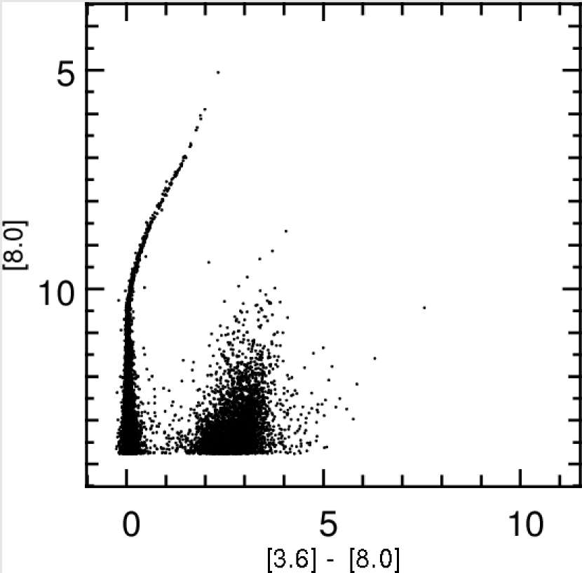
Figure 7: The [3.6]$-$[8.0] $vs.$ [8.0] color–magnitude diagram for the SWIRE survey toward the ELAIS N1 field which covers nine square degrees. The distribution and number (see text and Table 2) of faint, red galaxies are similar to that for the SAGE LMC survey (Figure 5). The curved blue sequence is presumably due to non–linearity in the [3.6] counts due to the 30s SWIRE exposures (SAGE uses 0.6s exposures to obtain linear data in this range). The SWIRE sources are limited to the SAGE brightness limit in Figure 5.

A large fraction of the faint red objects appear to be background galaxies. One of the SWIRE fields is plotted in Figure 7. This CMD looks qualitatively the same as Figure 5 in the region fainter than [8.0] $=$ 10 mag and for [3.6]$-$[8.0] $>$ 1.5 mag; the distribution of magnitudes and colors is similar including the rather sharp redward cut–off at [3.6]$-$[8.0] $=$ 3.5 mag and the small number of sources brighter than [8.0] $=$ 11 mag. The SAGE data have more counts per square degree than all the SWIRE fields. This suggests some of the faint, red objects belong to the LMC; however a definitive count of the LMC background will require observations in fields near the LMC. Indeed, the surface density of the putative background population towards the LMC appears uniform (magenta and cyan points, Figure 1) compared to the LMC stellar populations.

3.2.2 [8.0]$-$[24] $vs.$ [24]

Moving to longer wavelengths, the [8.0]$-$[24] $vs.$ [24] diagram (Figure 6) further compresses the bluer stellar sequences such that only stars with very strong emission in [24] stand out. In Figure 6, Spitzer IRS photometry is over–plotted on the SAGE data for a sample of sources investigated by Markwick–Kemper et al. (2006). Many of these are highly obscured objects. Markwick–Kemper et al. (2006) have classified the objects according to the scheme of Kraemer et al. (2002). This scheme identifies objects with silicate features in the circumstellar envelope (“S”, typically O–rich stars in the LMC, but could also be young, embedded stars) and carbonaceous features (“C”, typically C–stars). In addition, objects can be classified as planetary nebulae (PNe or “P”).

The population of sources identified above with background galaxies (same sources from the [3.6]$-$[8.0] $vs.$ [8.0] CMD with no $J-$band counterparts, cyan points) is well differentiated from stars in this diagram. We have argued above that most of these are probably background galaxies (the brightest sources include known LMC objects; see below). It is clear that our counts for [24] are not complete for all [8.0]$-$[24] as evidenced by the sloping cut–off at the red limit of Figure 6 for [24] $<$ 11 mag and [8.0]$-$[24] $>$ 3 mag. Nevertheless, a comparison to the SWIRE data shows that we should expect approximately 200–400 galaxies per square degree (see Table 2) with 7 $<$ [24] $<$ 11 mag. This compares with approximately 250 per square degree for the SAGE data.

As mentioned in the preceding section, some LMC YSOs are expected to be included in the SAGE source counts at all brightness levels. This can already be verified for the brightest, reddest objects. The IRS sources plotted in Figure 6 include four “S” objects which are generally the brightest, reddest objects and lie in the part of the CMD where massive YSOs are expected (Whitney et al., 2004; Meixner et al., 2006). Two of these sources are associated with young objects and may indeed be embedded, massive YSOs. Source MSX LMC 1200, the brightest “S” source in Figure 6, is identified as a likely compact H II region by van Loon et al. (2001). Source MSX LMC 1786 is identified with a molecular cloud (Johansson et al., 1998) by Egan et al. (2001). The other two “S” sources (MSX LMC 906 and MSX LMC 1436) have no further identification apart from 2MASS catalog id’s. Model colors and magnitudes for massive YSOs (Whitney et al., 2004) also show that these objects can have the same colors as those near the bright, red end of the “extreme” star sequences in Figures 5 and 6, though such objects should be rare even compared to AGB stars. The context, i.e. whether an object is found in or around a region of star formation, will be important in determining the it’s precise nature (particularly those sources which are completely obscured at shorter wavelengths).

The narrow vertical sequence at [8.0]$-$[24] $=$ $-0.2$ is composed predominantly of stars with $J-$[8.0] $\leq$ 1.0 (i.e. blue LMC stars and foreground objects). A sequence of points falls near [24] $=$ 10 but in between the main stellar and extragalactic loci. These sources have blue colors at shorter wavelengths and so are not obvious on any of the previous diagrams as they merge with the numerous LMC AGB stars at shorter wavelengths. But the sequence stands out at 24 $\mu$m, trending to larger values of [8.0]$-$[24] excess (see Figure 6 and the tip of the sequence marked by an “F”). This sequence is discussed further below.

4 Discussion

The Hess diagrams and CMDs presented in Figures 3–6 can be used to assess the relative importance to the mass loss budget in the LMC. Detailed model calculations will be made once the full SAGE data set is in hand and there are appropriate template spectra to assess the stellar envelope dust properties as a function of location in these diagrams. The SAGE team and others have existing and planned Spitzer and ground based spectroscopic follow–up programs underway. Some of the brightest mass–losing sources in the LMC have already been analyzed (see, for example, Zijlstra et al., 2006). These sources are prolific, but rare mass–losing objects. The full impact of the less luminous stars on the AGB has yet to be quantified.

The effect of dust in shaping the infrared CMDs is clear at a glance from Figures 3–6 and considering the 2MASS $H-K$ $vs.$ $K$ CMD (Nikolaev & Weinberg, 2000). In the latter, even at $Ks$ (2.1 $\mu$m), the tail of extreme AGB stars decreases in brightness for redder colors. This suggests the primary effect at short wavelengths is circumstellar extinction. In the $J-$[3.6] $vs.$ [3.6] diagram of Figure 3, the extreme star branch has essentially constant brightness. By 8 $\mu$m, the sequence is increasing in brightness clearly indicating that the circumstellar envelopes are exhibiting successively more excess emission. The [8.0]$-$[24] $vs.$ [24] CMD shows that the majority of the reddest objects are the fainter objects we have identified with background galaxies. However, at the brightest and reddest this sequence seems to merge with the luminous stellar sources (i.e. the “extreme” AGB and SG stars). Indeed a survey of the SIMBAD catalog shows a number of these objects to be PNe and other bright, stellar, IRAS sources (one Wolf–Rayet star and several objects associated with HII regions, as well as obscured AGB stars). Of the 236 sources with [8.0]$-$[24] $>$ 3.0 mag and [24] $<$ 7.0 mag, 10 are known PNe and 13 are classified as IRAS or IR sources (of which Loup et al., 1997, discuss four as obscured AGB stars), The majority have no other counterparts in the SIMBAD data base.

This general picture is confirmed by the Spitzer IRS sources plotted in Figure 6. The stars identified as “C” lie among the “extreme” stars where many C–rich objects are expected. The “S”, or silicate, sources lie among these, but also slightly to the red and at brighter magnitudes where the M supergiants (green points) and luminous AGB stars predominate. The IRS PNe lie at bright magnitudes and red colors as do several massive YSOs as discussed in § 3.2.2. Clearly SAGE will provide a host of new mass losing objects to follow up in detail.

While there are differences in detail, the location of the basic LMC AGB and supergiant sequences correspond remarkably well to those predicted from Galactic models (moved to the distance of the LMC, distance modulus$=$18.5) for the analogous objects (Wainscoat et al., 1992; Cohen, 1993, 1994, 1995). In particular, this includes the general location, extent, and slope of the “extreme” AGB stars in Figures 3 and 4, as well as the position of the most luminous supergiants and O–rich objects above the extreme stars. The predicted positions of the Galactic objects such as PNe and HII regions are also in rough agreement with the objects identified above in the [8.0]$-$[24] $vs.$[24] CMD (Figure 6).

Figure 3 shows the most dominant Spitzer population by number is the red giants. The RGB is the most densely populated sequence with a tip magnitude of TRGB([3.6])$=$ 11.85. There are approximately 650000 stars on the RGB below the TRGB in the epoch one data set. The peak number density (2400 stars in a 0.0475$\times$0.0625 square magnitude pixel) occurs at $J-$[3.6], [3.6] $=$ 0.8, 15.6. The RGB number density drops rapidly to a value $\sim$ 25$\%$ of its value just to the faint side of the tip. Approximately 74$\%$ of the stars in the $J-$[3.6] $vs.$ [3.6] CMD above the TRGB are O–rich, C–rich, and SG types. Roughly 12$\%$ of stars above the TRGB are foreground giants and dwarfs with the remainder being mostly blue LMC supergiants according to the discussion in §3.

The AGB stars and supergiants can be divided up among those with strong mass loss (the so called “extreme” stars) and those whose colors suggest weaker mass loss or less dusty envelopes. Of the latter, most of the objects can be classified as O–rich or C–rich based on the $J-K$ $vs.$ $K$ classification of Cioni et al. (2006). The red tail of C–stars (literally where Figure 3 shows red points) stretches to approximately $J-$[3.6] $=$ 3.1 where the density of objects drops significantly toward redder colors (see Figure 3). This color limit is a useful indicator of the extreme or obscured AGB stars as it corresponds roughly to the point in the $J-K$ $vs.$ $K$ CMD where the AGB stars become fainter at redder color (exhibiting strong circumstellar extinction). The C/O star ratio (not including the “extreme” stars) is 0.39 (see Table 1). This value is somewhat lower than given by Cioni et al. (2006); however, the data analized by Cioni et al. (2006) includes stars at over a larger area than considered here and for which the number of C–stars is significant. A full analysis of the C/O star ratio with position will follow in a subsequent paper.

According to the models of Marigo et al. (2003), the position of the C–stars in the red tail (Marigo et al., 2003, discuss this in terms of $J-K$) is due to cooler temperatures resulting from their molecular opacity differences compared to the O–rich stars. The opacity difference is a direct result of the changing molecular equilibrium as dredge up changes the ratio of C/O (and hence the important molecular constituents in the C–rich phase compared to the O–rich phase). The colors are thus “photospheric” in nature, and not until the obvious break in the CMDs (e.g., $J-$[3.6] $=$ 3.1) does dust significantly affect the colors. The majority of stars in the red tail of Figure 3 are optically visible C–stars with objective prism identifications given by Blanco & McCarthy (1990) and Kontizas et al. (2001). About 25$\%$ of the sources identified as C–stars here have no previous identification in the SIMBAD database (but are 2MASS sources).

Comparison of the [3.6]$-$[8.0] $vs.$ [8.0] and [8.0]$-$[24] $vs.$ [24] CMDs suggests the relative importance of mass loss can be seen among the different AGB stars. The green SGs lie to the blue of the yellow extreme stars in the former diagram, but generally to the red in the latter. The SGs thus appear to have cooler, perhaps more extended, dust envelopes. The red “visible” C–stars generally have little or no 24 $\mu$m excess, whereas a subset of the blue O–rich AGB stars exhibit increasing amounts of excess emission and presumably mass loss. This sequence is approximately at constant [8.0] magnitude ($\approx$ 10.5). This group of AGB stars is well above the TRGB in the shorter wavelength CMDs and represents the brightest tip of stars classified as O–rich just at the transition to the “visible” C–star locus in the $J-$[8.0] $vs.$ [8.0] CMD (Figure 4). The group of stars is clearly visible as a slight enhancement in density in the Hess diagram (Figure 4) above and to the red of the thin finger of AGB stars which rise above the TRGB (i.e. at $J-$[8.0], [8.0] $\approx$ 1.5, 10.5). Fainter O–rich AGB stars are not detected at high signal–to–noise in this preliminary data set at 24 $\mu$m. Even so, this is striking evidence for mass loss in lower luminosity stars than has generally been explored in the LMC.

Van Loon et al. (1999) derived mass loss rates from a sample of 57 stars in the LMC chosen by their infrared excess. Their analysis suggests lower luminosity AGB stars have mass loss rates $\mathrel{\hbox{\hbox to0.0pt{\hbox{\lower 4.0pt\hbox{$\sim$}}\hss}\hbox{$>$}}}$10^-7 M_⊙ yr^-1. The SAGE 24 $\mu$m data reach somewhat below the luminosities probed by van Loon et al., and the epoch one data will be combined with epoch two photometry, allowing SAGE to reach even fainter sources at 24 $\mu$m (0.4 mag). The fact that the low luminosity mass losing sources we have identified above (Figure 6, “F”) span a range of 24 $\mu$m excess from no excess to $\sim$ 2 mag suggests they represent the faintest population of dusty sources with significant mass loss (10^-7 $\mathrel{\hbox{\hbox to0.0pt{\hbox{\lower 4.0pt\hbox{$\sim$}}\hss}\hbox{$>$}}}$M_⊙ yr^-1 $\mathrel{\hbox{\hbox to0.0pt{\hbox{\lower 4.0pt\hbox{$\sim$}}\hss}\hbox{$>$}}}$10^-8) in the LMC. Thus, the full SAGE catalog should detect the all the important mass losing sources in the LMC. Adding up the first epoch SAGE sources identified here as “extreme” AGB stars, SG/luminous AGB, and the present lower luminosity O–rich AGB stars, we find approximately 10$\%$ of the evolved stars above the TRGB are likely significant mass–loss sources.

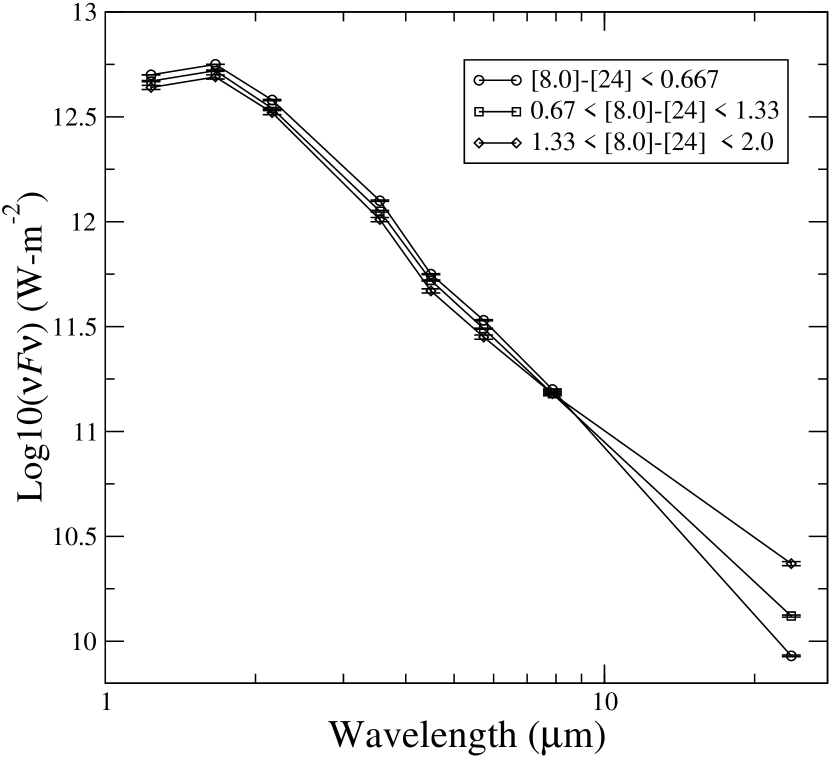
Figure 8: Spectral energy distributions (SED) for the average source in each of three [8.0]$-$[24] color bins as indicated in the plot. The SEDs are very similar until 8 $\mu$m. The 24 $\mu$m flux increases suggesting a sequence of stars at the tip of the AGB (see text and Figures 3 and 4) exhibiting increasing amounts of mass loss from a “bare” AGB star (open circles) to an AGB star with a cool circumstellar envelope (open diamonds). The error bars represent the error in the mean for the average photometry in each color bin constructed from 632, 439, and 75 stars (see text).

In Figure 8, the average spectral energy distribution (SED) is plotted for these low luminosity AGB sources. The sample of stars is arbitrarily divided into three bins of varying [8.0]$-$[24] color ([8.0]$-$[24] $\leq$ 0.67, 0.67 $\leq$ [8.0]$-$[24] $<$ 1.34, 1.34 $\leq$ [8.0]$-$[24] $<$ 2.0) to show the increasing excess emission along the sequence at constant 8 $\mu$m brightness. There are 632, 439, and 75 stars in these bins, respectively. To contribute to a given bin, a star is required to have valid photometry for each 2MASS, IRAC, and MIPS (24 $\mu$m) band; hence, there are more stars plotted in Figure 6 than represented in Figure 8 since the former includes objects for which there is no required $H$, [4.5], or [5.8] photometry.

The sources in all bins have very similar SEDs up to 8 $\mu$m, but then exhibit increasing 24 $\mu$m flux indicative of successively more cool dust emission which we suggest is due to increasing mass loss among otherwise very similar objects. Careful scrutiny of Figure 8 shows that the stars with the least amount of 24 $\mu$m excess are the brightest at shorter wavelengths, while those with the most excess are fainter at the shorter wavelengths. The cool dust envelopes are likely providing additional extinction at the shorter wavelengths. While not shown in the figure, arbitrarily scaling the SEDs to match in the near infrared shows that they are nearly identical until about 6.8 $\mu$m. At this point, a clear but small excess begins to show at 8 $\mu$m. This fact, and the fact that no fainter population of obvious mass losing stars is evident in the much deeper CMD shown in Figure 4 provides support for our claim that SAGE will detect all the important mass losing sources in the LMC.

Could these objects be chance alignments of “normal” AGB stars and background (dusty) galaxies at 24 $\mu$m? To estimate the possible number of chance alignments, consider the SWIRE number counts given above. The IRAC–24 $\mu$m search radius was 1^′′. The total area covered by all 24 $\mu$m sources is then 28000 sources $\times$ the area per 24 $\mu$m source $=$ 0.007 square degrees. Multiplying this by the number of SWIRE galaxies per square degree (253) gives two chance alignments per 28000 24 $\mu$m sources).

5 Summary

Epoch one data for the SAGE survey of the entire LMC have been presented for the Spitzer IRAC bands and the MIPS 24 $\mu$m band. For the first time, an infrared view is presented which places the bright IRAS and MSX sources in context. The Spitzer (and 2MASS) CMDs are dominated by red giants (650000 red giants to the present epoch one limit of the survey) and AGB stars.

For epoch one of the SAGE survey, we find approximately 18000 oxygen–rich AGB stars, 7000 carbon–rich stars, 1200 late–type supergiants (or luminous oxygen–rich stars), and 1200 “extreme” AGB stars (optically obscured or enshrouded AGB stars) which represent the high mass loss rate evolved star population in LMC. Of the approximately 30000 evolved stars above the tip of the red giant branch, some 10$\%$, can be readily identified with dusty mass–losing envelopes. The C/O star ratio is approximately 40$\%$ (46$\%$ if all the “extreme” stars are considered as C–rich). This is an average value which can be compared to the C/O star ratio maps of Cioni et al. (2006) which give a range of approximately 0.2–0.6.

The 24 $\mu$m channel of the MIPS instrument clearly shows that lower luminosity AGB stars (which are not remarkable at IRAC wavelengths) have excess emission indicating cool dusty envelopes and mass loss. This population has been largely unexplored to date, and SAGE will be uniquely powerful in allowing a quantitative assessment of its overall impact on the LMC.

Approximately 12$\%$ of the stars above the tip of the red giant branch are foreground dwarfs and giants. The Hess diagrams suggest the relative contamination should be less at fainter magnitudes. Extragalactic populations stand out in the longer wavelength color–magnitude diagrams (those which include 8 $\mu$m and 24 $\mu$m data points) as objects with fainter magnitudes and red colors (perhaps in part due to excess PAH emission at these wavelengths), but the numbers are not large compared to the total. This background contribution agrees well with published Spitzer galaxy counts in other fields of view.

The authors would like to acknowledge useful discussions with Mark Dickinson about SWIRE and the background galaxy counts. The plots and analysis in this article made use of the Yorick programing language. This article made use of the SIMBAD database at the CDS, and this research has been funded by NASA/SST grant 1275598 and NASA grant NAG5–12595. The authors would also like to acknowledge the comments of an anonymous referee regarding stellar crowding the relation between IRAC and MIPS sources. Addressing these comments has strengthened our results.

6 Appendix

Given the difference in IRAC and MIPS point spread function (PSF) size (2^′′ and 6^′′, respectively), the issue of source matching between the two and the impact of crowding on the color–magnitude diagrams (CMD) needs to be addressed. In §2, we described the matching of MIPS and IRAC sources within a 1^′′ radius. In the case of multiple sources, the closer source is assumed to be the appropriate match. Depending on the level of crowding of IRAC sources within the MIPS PSF, this matching technique could associate a fainter IRAC source with the sum of multiple MIPS 24 $\mu$m sources leading to spurious red colors (for example in the finger of low luminosity oxygen rich asymptotic giant branch, AGB, stars discussed in §4).

In order to quantify the effect of the multiple IRAC sources within the MIPS PSF we re–ran the matching of IRAC and MIPS sources with a 6^′′ radius (i.e, twice the size of the MIPS PSF full width at half maximum). This matching resulted in a total of approximately 30000 sources (10$\%$ more than the previous matching discussed in §2). The distribution of offsets was similar to the original with a tail to larger matches out to $\sim$ 6^′′. The mean offset changed from 0.4^′′ to 0.7^′′ and the systematic offsets in RA and Dec between the two datasets remained much less than 0.1^′′ as before.

Two MIPS sources had as many as five matches within this new large radius, four MIPS sources had four matches, 41 MIPS sources were matched with three IRAC sources, and 1058 MIPS sources had two IRAC matches. The ratio of the sum of 8 $\mu$m flux due to all sources in the 6^′′ radius to that of the chosen match (closest source) was less than 1.5 in more than half of all of the multiple source cases while 248 matches had flux ratios greater than 2.0. The number of double matches is sufficient enough to be interesting since some of the sequences identified in the CMDs above had a similar number of stars identified.

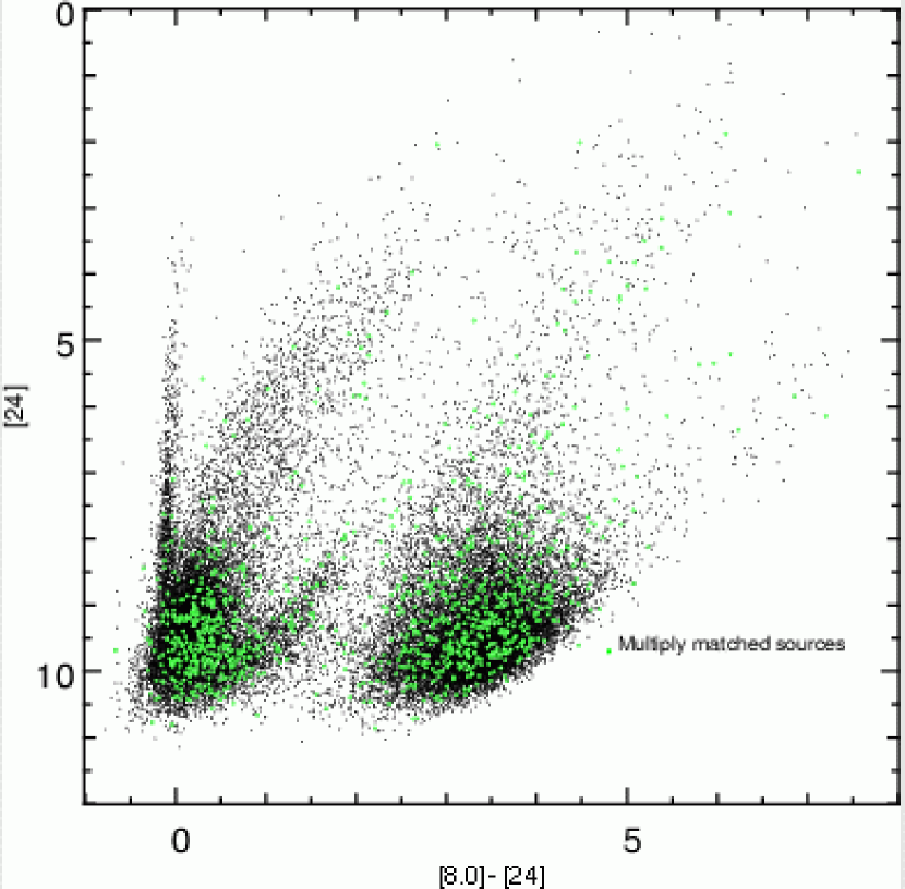
Figure 9: The [8.0]$-$[24] $vs$ [24] color–magnitude diagram (CMD). This is the same as Figure 6, except for an IRAC–MIPS matching radius of 6^′′. A few percent of all the matches have multiple IRAC sources within the larger radius used to find a MIPS 24 $\mu$m source (green dots). The majority of multiples are double with about 50 triple matches, four quadruple, and two quintuple. The distribution of matches suggests the stellar sources and background galaxies are similarly affected in the CMD, and the total number of multiply matched sources for any sequence in the CMD is small: there are 30000 black points in this diagram and 1103 green points. See the appendix for details.

To assess the impact of the multiple sources, they are overplotted on the [8.0]$-$[24] $vs$ [24] color–magnitude diagram (CMD) in Figure 9. It is immediately clear that the multiply matched sources sample the CMD uniformly. Because their number is only 3.7 $\%$ percent of the total, we conclude that they have no significant impact on the sequences of stars in the CMD. The bulk of multiple sources lie in the region of highest source density in the “bar” feature of the LMC. Plotting the CMD for sources in the less crowded region above the bar shows that all the prominent features of the CMD described in the text remain.

This conclusion is based on the assumption that the IRAC 8 $\mu$m counts are complete for the magnitude range considered. This is indeed the case. Figure 10 shows the 8 $\mu$m luminosity function for all the IRAC 8 $\mu$m sources in the SAGE epoch 1 data presented here (approximately 260000) sources. The maximum source density is approximately 45000 per square degree and the counts are rising to [8.0] $=$ 13 mag (about two full magnitudes below the faintest stellar sources in Figure 6). The 8 $\mu$m crowding limit can be explicitly calculated following the formalism of Olsen et al. (2003). The 8 $\mu$m maximum surface density results in a 17 magnitude per square arcsecond surface brightness for the luminosity function shown in Figure 10. Extrapolating the source counts to 38th magnitude results in a surface brightness of 16.6 magnitudes per square arcsecond. Following the prescription of Olsen et al. (2003), this latter surface brightness results in crowding induced errors of only 2$\%$ in the [8.0] photometry to [8.0] $=$ 10.5 mag for a 2^′′ IRAC PSF. Thus the 8 $\mu$m counts should be nearly 100 $\%$ complete at the magnitude level represented in Figure 6, and the chance of associating a spurious faint 8 $\mu$m source with multiple 24 $\mu$m sources in the MIPS beam is negligible.

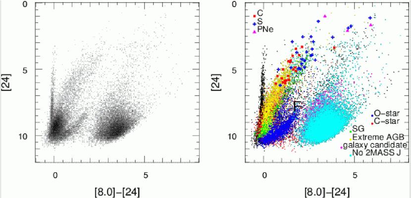
Figure 6: Same as Figure 5, but for the [8.0]$-$[24] $vs.$ [24] color–magnitude diagram and Hess diagram. The brightest cyan points ([24] $\mathrel{\hbox{\hbox to0.0pt{\hbox{\lower 4.0pt\hbox{$\sim$}}\hss}\hbox{$<$}}}$7) correspond to luminous LMC stars and other objects such as planetary nebulae and young emission–line sources. A number of the cyan objects lie at the tip of the yellow extreme asymptotic giant branch (AGB) star sequence and thus are likely luminous AGB stars that are completely obscured at shorter wavelengths. This picture is confirmed by the plotted Spitzer IRS spectroscopy sources, “C”, “S”, and “PNe” which indicate carbonaceous, silicate, and PNe features, respectively (see text for details). As in Figure 5, most of the cyan points ([24] $\mathrel{\hbox{\hbox to0.0pt{\hbox{\lower 4.0pt\hbox{$\sim$}}\hss}\hbox{$>$}}}$7) are probably background galaxies (see text and Figure 2). The sequence of oxygen–rich (O–rich) AGB stars (blue dots) include a prominent “finger” reaching to [24], [8.0]$-$[24] $\sim$ 8.5, 2.0. These are O–rich stars at nearly constant [8.0] magnitude (10.5, see Figure 4 and 8) at the tip of the AGB which appear to have increasing amounts of mass–loss (see text). The tip of this finger is indicated with an “F” in the plot.

Figure 10: The 8 $\mu$m luminosity function for all 8 $\mu$m sources in the present epoch 1 dataset. This luminosity function is used to show that the data in Figures 6 and 9 are not significantly affected by point source crowding. See the appendix for details.

Table 1: Spitzer SAGE Stellar Populations

Population	Diagram	Number of Sources	$\%$ of Total	Figure Color
Point sources with both $J$ and [3.6]	$J-$[3.6] $vs.$ [3.6]	821305	100	black
Red giant branch stars	$J-$[3.6] $vs.$ [3.6]	650000	79
Point sources brighter than TRGB	$J-$[3.6] $vs.$ [3.6]	42897	5
Carbon–rich AGB stars	$J-$[3.6] $vs.$ [3.6]	6935	1	red
Oxygen–rich AGB stars	$J-$[3.6] $vs.$ [3.6]	17875	2	blue
Supergiant/luminous Oxygen rich AGB	$J-$[3.6] $vs.$ [3.6]	1240	0.1	green
Extreme AGB stars	$J-$[8.0] $vs.$ [8.0]	1228	0.1	yellow
Galactic foreground brighter than TRGB	$J-$[3.6] $vs.$ [3.6]	4995	1
Background galaxy candidates I	$J-$[8.0] $vs.$ [8.0]	1887	1	magenta
Background galaxy candidates II	[3.6]$-$[8.0] $vs.$ [8.0]	17735	7	cyan
24 $\mu$m sources with IRAC counterparts	[8.0]$-$[24] $vs$ [24]	27741	100	black
Faint Oxygen–rich AGB stars with mass loss	[8.0]$-$[24] $vs.$ [24]	1158	4	blue

Table 2: Background Galaxy Counts

Field	[8.0] Counts deg-2	[24] Counts deg-2
SWIRE ELAIS N1	288	372
SWIRE ELAIS N2	153	160
SWIRE ELAIS S1	183	224
SWIRE XMM	231	299
SWIRE Chandra DFS	214	278
SWIRE Lockman Hole	247	321
SAGE	400	253

References

- Benjamin et al. (2003) Benjamin, R.A., et al. 2003, PASP, 115, 953
- Bertin & Arnouts (1996) Bertin, E., & Arnouts, S. 1996, A&AS, 117, 393
- Blanco & McCarthy (1990) Blanco, V. M., & McCarthy, M. F. 1990, AJ, 100, 674
- Blum et al. (1995) Blum, R. D., Carr, J. S., Sellgren, K., & Terndrup, D. M. 1995, ApJ, 449, 623
- Cioni et al. (2003) Cioni, M.-R. L., et al. 2003, A&A, 406, 51
- Cioni et al. (2006) Cioni, M.-R. L., Girardi, L., Marigo, P., & Habing, H. J. 2006, A&A, 448, 77
- Cohen (1993) Cohen, M. 1993, AJ, 105, 1860
- Cohen (1994) Cohen, M. 1994, AJ, 107, 582
- Cohen (1995) Cohen, M. 1995, AJ, 444, 874
- Cohen et al. (2003) Cohen, M., Megeath, T.G., Hammersley, P.L., Martin—Luis, F., & Stauffer, J. 2003, AJ, 125, 2645
- Dale et al. (2005) Dale, D. A., et al. 2005, ApJ, 633, 857
- Diolaiti et al. (2000) Diolaiti, E., Bendinelli, O., Bonaccini, D., Close, L., Currie, D., & Parmeggiani, G. 2000, A&AS, 147, 335
- Egan et al. (2001) Egan, M. P., Van Dyk, S. D., & Price, S. D. 2001, AJ, 122, 1844
- Elias, Frogel, & Humphreys (1985) Elias, J. H., Frogel, J. A., & Humphreys, R. M. 1985, ApJS, 57, 91
- Engelbracht et al. (2006) Engelbracht, C. et al. 2006, in preparation
- Epchtein et al. (1994) Epchtein, N., et al. 1994, Ap&SS, 217, 3
- Fazio et al. (2004) Fazio, G. G., et al. 2004, ApJS, 154, 39
- Gaustad et al. (2001) Gaustad, J. E., McCullough, P. R., Rosing, W., & Van Buren, D. 2001, PASP, 113, 1326
- Gordon et al. (2005) Gordon, K., et al. 2005, PASP, 117, 503
- Harris & Zaritsky (2001) Harris, J., & Zaritsky, D. 2001, ApJS, 136, 25
- Holtzman et al. (1999) Holtzman, J. et al. 1999, AJ, 118, 2262
- Hughes & Wood (1990) Hughes, S. M. G., & Wood, P. R. 1990, AJ, 99, 784
- Johansson et al. (1998) Johansson, L. E. B., et al. 1998, A&A, 331, 857
- Kontizas et al. (2001) Kontizas, E., Dapergolas, A., Morgan, D. H., & Kontizas, M. 2001, A&A, 369, 932
- Kraemer et al. (2002) Kraemer, K. E., Sloan, G. C., Price, S. D., & Walker, H. J. 2002, ApJS, 140, 389
- Lonsdale et al. (2004) Lonsdale, C., et al. 2004, ApJS, 154, 54
- Loup et al. (1997) Loup, C., Zijlstra, A. A., Waters, L. B. F. M., & Groenewegen, M. A. T. 1997, A&AS, 125, 419
- Marigo et al. (2003) Marigo, P., Girardi, L., & Chiosi, C. 2003, A&A, 403, 225
- Markwick–Kemper et al. (2005) Markwick–Kemper, F., Leisenring, J., Meixner, M., van Dyk, S., & Szczerba, R. 2005, IAU Symposium, 231, 134
- Markwick–Kemper et al. (2006) Markwick–Kemper, F., Leisenring, J., Meixner M., Van Dyk S. D., Speck, A.K., Dijkstra, C., Szczerba R., Cami, J., & Ueta T. 2006, in preparation.
- Massey (2002) Massey, P. 2002, ApJS, 141, 81
- Meixner et al. (2006) Meixner, M. et al. 2006, submitted to the AJ
- Mouhcine & Lançon (2003) Mouhcine, M., & Lançon, A. 2003, MNRAS, 338, 572
- Neugebauer et al. (1984) Neugebauer, G., et al. 1984, ApJ, 278, L1
- Nikolaev & Weinberg (2000) Nikolaev, S., & Weinberg, M. D. 2000, ApJ, 542, 804
- Olsen (1999) Olsen, K. A. G. 1999, AJ, 117, 2244
- Olsen et al. (2003) Olsen, K. A. G., Blum, R. D., & Rigaut, F. 2003, AJ, 126, 452
- Price et al. (2001) Price, S. D., Egan, M. P., Carey, S. J., Mizuno, D. R., & Kuchar, T. A. 2001, AJ, 121, 2819
- Reach et al. (2005) Reach, W. T., et al. 2005, PASP, 117, 978
- Schwering (1989) Schwering, P. B. W. 1989, A&AS, 79, 105
- Smith et al. (1987) Smith, A. M., Cornett, R. H., & Hill, R. S. 1987, ApJ, 320, 609
- Stetson (1987) Stetson, P. B. 1987, PASP, 99, 191
- Skrutskie et al. (2006) Skrutskie, M. F., et al. 2006, AJ, 131, 1163
- van Loon et al. (1999) van Loon, J. T., Groenewegen, M. A. T., de Koter, A., Trams, N. R., Waters, L. B. F. M., Zijlstra, A. A., Whitelock, P. A., & Loup, C. 1999, A&A, 351, 559
- van Loon et al. (2001) van Loon, J. T., Zijlstra, A. A., Bujarrabal, V., & Nyman, L.-Å. 2001, A&A, 368, 950
- van Loon et al. (2005) van Loon, J. T., Cioni, M.-R. L., Zijlstra, A. A., & Loup, C. 2005, A&A, 438, 273
- Wainscoat et al. (1992) Wainscoat, R. J., Cohen, M., Volk, K., Walker, H. J., & Schwartz, D. E. 1992, ApJS, 83, 111
- Whitney et al. (2004) Whitney, B. A., Indebetouw, R., Bjorkman, J. E., & Wood, K. 2004, ApJ, 617, 1177
- Zaritsky et al. (2004) Zaritsky, D., Harris, J., Thompson, I.B. & Grebel, E.K. 2004, AJ, 128, 1606
- Zijlstra et al. (2006) Zijlstra, A. A., et al. 2006, astroph/0602531