Comparison of Magnetic Field Structures on Different Scales in and around the Filamentary Dark Cloud GF 9

Abstract

New visible polarization data combined with existing IR and FIR polarization data are used to study how the magnetic field threading the filamentary molecular cloud GF 9 connects to larger structures in its general environment. We find that when both visible and NIR polarization data are plotted as a function of extinction, there is no evidence for a plateau or a saturation effect in the polarization at $A_{\rm V}\approx$ 1.3 as seen in dark clouds in Taurus. This lack of saturation effect suggests that even in the denser parts of GF 9 we are still probing the magnetic field. The visible polarization is smooth and has a well-defined orientation. The IR data are also well defined but with a different direction, and the FIR data in the core region are well defined and with yet another direction, but are randomly distributed in the filament region. On the scale of a few times the mean radial dimension of the molecular cloud, it is as if the magnetic field were ‘blind’ to the spatial distribution of the filaments while on smaller scales within the cloud, in the core region near the IRAS point source PSC 20503+6006, polarimetry shows a rotation of the magnetic field lines in these denser phases. Hence, in spite of the fact that the spatial resolution is not the same in the visible/NIR and in the FIR data, all the data put together indicate that the field direction changes with the spatial scale. Finally, the Chandrasekhar and Fermi method is used to evaluate the magnetic field strength, indicating that the core region is approximately magnetically critical. A global interpretation of the results is that in the core region an original poloidal field could have been twisted by a rotating elongated (core$+$envelope) structure. There is no evidence for turbulence and ambipolar diffusion does not seem to be effective at the present time.

1 Introduction

With the measurement of visible linear polarization of field stars, followed by developments of Near and Far Infrared (respectively NIR and FIR) and submillimetric polarimetry, it is now possible to trace magnetic field structures from the scale of the Milky Way to that of star forming regions and cores. In the diffuse Interstellar Medium (ISM), the general assumption that elongated dust grains usually have their smallest axis aligned in a direction comparable to that of the local magnetic field has lead to a toroidal representation of the Galactic magnetic field. A similar topology of the magnetic field can also sometimes be observed in other galaxies (e.g. Scarrott et al. (1990)). On the smaller scales of molecular clouds, a similar relation exists between grain alignment and magnetic field directions (see Lazarian (2003) for an exciting review on the subject) and many topologies of the magnetic field are suspected to exist. Among others, helicoidal, toroidal, poloidal and hourglass configurations have been proposed to interpret observed polarization patterns, taking care of the physical conditions in these environments (e.g., Orion A, M17). However, one of the most important limitations of linear polarimetry is that we only get a two-dimensional projected average representation of the magnetic field topology because of the integration on the plane of the sky of the contribution to the polarized emission due to each aligned grain, or its dichroic absorption for visible/NIR observations. This leads to a degeneracy problem since many three dimensional (3D) topologies of the field can produce identical polarization patterns. A method to get rid of this degeneracy problem is the use of models. On the scale of relatively nearby filamentary molecular clouds and cores, this method has been used and allows in some cases to select one field topology among many possible ones (e.g., Matthews et al. (2001), Vallée et al. (2003)).

In addition to models, other diagnostics of magnetic fields can be used to lift the degeneracy due to the plane-of-sky integration. When column densities are high enough, observations of the Zeeman effect can yield the line-of-sight component of the magnetic field strength (e.g. Crutcher (1999)). Finally, by determining the ion-to-neutral molecular line-width ratio in non turbulent regions with a linear flow, it is possible to determine the angle between the field direction and the line of sight (Houde et al. (2000a), Houde et al. (2000b), Houde et al. (2001)). By combining all three methods together, we get the 3D field topology (e.g., Houde et al. (2002) for M17, Houde et al. (2004) for Orion A). The observation of Zeeman splitting of spectral lines requires bright dense cores, but even in other regions, it is possible to get the 3D geometry of the field even if the field strength is unknown.

These methods can inform us about how magnetic fields can contribute to cloud dynamics, but our ultimate goal is to understand the competition between gravitational, thermal, magnetic, and turbulent forces. More specifically, magnetic fields and turbulence are both competing to slow down the star formation process, otherwise stars would form much faster than observations show. Combining polarization modeling techniques (e.g., Fiege & Pudritz (2000)) and predictions for magnetized simulations of turbulence (e.g., Heitsch et al. (2001), Padoan et al. (2001)), one can hope to be able to determine the relative contributions of magnetic fields and turbulence.

To reach this goal, and to understand how magnetic fields thread the dark filaments, and to put observational constraints on modeling we propose to make comparisons of magnetic fields as seen in and around individual objects. This approach, namely a multi-scale analysis of the magnetic field, has begun to be done via comparisons of visible, NIR, FIR and/or submm polarization data in the OMC1 (Schleuning (1998)), OMC3 (Matthews et al. (2001)) and GF 9 regions (Jones (2003)). In these works, aspects of the galactic magnetic field extending on tens of degrees are compared with aspects of the clouds probed in the densest regions of the clouds with resolutions $\sim 10^{\prime\prime}$, but there is generally a lack of information between these two scales. Here we present observations at an intermediate scale, as much as the presence of field stars allows it, to have a clearer view of the topology of the field at the interface ISM/filamentary molecular clouds. From a general point of view, this approach should provide new insights on the way magnetic fields and clouds are dynamically coupled and shaped. In this paper we address this problem for the GF 9 filamentary molecular cloud region. A forthcoming paper will address the more complex situation for the Orion A region.

A description of data available about GF 9 is given in section 2. Observations and observational results are presented in section 3. An analysis and a discussion follow in section 4, and our conclusions are given in section 5.

2 The GF 9 Region

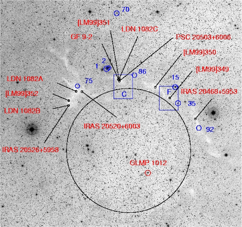
Figure 1: DSS red plate of GF 9 and its environment with reverse colors. Various regions appearing in catalogs are identified in the Figure. GLMP 1012 is a post AGB star (see text for explanations). Boxes are regions observed by Ciardi et al. (1998), Ciardi et al. (2000) with letters C and F indicating the core region and the filament regions respectively. Positions of stars S1, S2, S15, S35, S70, S75, S86 and S92 are shown. The ‘constellation’ formed by stars S75, S70, S86, S35 and S92 can be used to compare the polarization pattern shown in Figure 2 with the location of the densest regions of the ISM as seen in the visible. The great black circle suggests the circular shape of the GF 9 filaments. The densest parts of the ISM forming GF 9 are located to the north of this circle, and small faint clouds are located in the south.

The GF 9 dark filamentary structures have been catalogued first as B150 by Barnard (1927), L1082 by Lynds (1962) and GF 9 by Schneider & Elmegreen (1979). A first estimate of the distance to these condensations as $d=440$ pc was determined by Viotti (1969) (See Hilton & Lahulla (1995)) but an estimate of $d=200$ pc to the extreme class 0 object GF 9-2 based on star counts was reported more recently by Wiesemeyer (1998). The first estimate is reported in catalogs or works on relatively large core samples by Benson & Myers (1989), Goodman et al. (1993), Dobashi et al. (1994), Lee & Myers (1999), Furuya et al. (2003), while the second one is reported in works by André et al. (2000), Furuya et al. (2003) and Froebrich (2005). Assuming $d=200$ pc, GF 9-2 (see Figure 1) has a luminosity $L_{\rm bol}=0.3L_{\odot}$, an envelope mass $M_{\rm env}\sim 0.5M_{\odot}$, a ratio $L_{\rm submm}/L_{\rm bol}\sim 10\%$ and a bolometric temperature $T_{\rm bol}\leq 20$K. No outflow manifestation, nor structures are detected but infall motions are observed (Güsten (1994), Wiesemeyer (1997), Wiesemeyer (1998) and André et al. (2000)). GF 9-2 must be particularly young since it has a H₂O maser but no detected outflow (Furuya et al. (2003), Furuya et al. (2005)).

Two $\approx 8^{\prime}\times 10^{\prime}$ regions, namely GF 9-core and GF 9-fila, have been observed by Ciardi et al. (1998), Ciardi et al. (2000). The two areas are shown in Figure 1 by blue boxes identified by C and F. The GF 9-core region is associated with the IRAS point source class 0 protostar PSC 20503+6006, but also with GF 9-2 and an object named [LM99]351. JHK photometry of these two regions probe similar masses but the filament region is consistent with a uniform-density cylindrical cloud, while the core region contains a centrally condensed core with the highest extinction region lying to the north of the IRAS point source. CO, ¹³CO and CS surveys of these two regions give consistent views with these two pictures, but also reveal infall/outflow motions in order to explain CS line broadening in the core region where n${}_{\rm H_{2}}\approx 15000\pm 3000$ cm^-3 (assuming $d=440$ pc). In the filament region, n${}_{\rm H_{2}}\approx 6000\pm 1200$ cm^-3 (see Table 2 in Ciardi et al. (2000)). CO and NH₃ observations of three regions with an infrared association are presented by Benson & Myers (1989). These sources are IRAS 20520+6003, 20526+5958 and 20503+6006, and they are associated respectively with the LDN 1082A, B and C cores. An analysis of these data by Goodman et al. (1993) shows that motions consistent with uniform rotation in dense cores are present in LDN 1082A and LDN 1082B, while not in LDN 1082C. However recent works by Furuya et al. (2005) show a velocity gradient along the major axis in the core in GF 9-2 which could be due to a rotation of the core. ¹³CO observations by Dobashi et al. (1994) have also been done at 3 positions in GF 9. Referring to Lee & Myers (1999), objects named [LM99]349 and [LM99]350 (see figure 1) have no associated embedded young stellar objects (EYSO) while [LM99]351 ($\approx 1^{\prime}$ west of GF 9-2) and [LM99]352 have associated EYSO.

First $\lambda=184$ $\mu$m FIR polarimetry observations from space with ISO in GF 9 were done in the core and filament regions by Clemens et al. (1999). Additional measurements at $\lambda=1.65$ $\mu$m on 9 stars shining through the same regions of GF 9 are also reported by Jones (2003). Finally, 850 $\mu$m polarimetry observations were done at the JCMT by Jane S. Greaves in 1998 at one position in the filament.

Initially, the relatively small heliocentric distance of GF 9, its filamentary shape, and potentially interesting FIR measurements in this region were the major factors which motivated us to conduct visible polarimetry around these filamentary dark structures.

3 Observational results

3.1 Observations

The observations were carried out on the 1.6 m telescope at the Observatoire du Mont-Mégantic (OMM), Québec, Canada, between 2000 September and 2003 July using a 8.2 arcsecond aperture hole and a broad band red filter (RG645: 7660 Å central wavelength, 2410 Å FWHM). Polarization data were taken with Beauty and the Beast, a two-channel photoelectric polarimeter, which uses a Wollaston prism, a Pockels cell, and an additional quarter wave plate. The data were calibrated for polarization instrumental efficiency, instrumental polarization (due to the telescope mirrors) and zero point of position angles using a prism, non polarized and polarized standard stars, respectively. On average, the instrumental polarization was $0.081\pm 0.061\%$ and was subtracted. The observational errors were calculated from photon statistics and also include uncertainties introduced by the previously mentioned calibrations. The final uncertainty on individual measurements of the polarization $P$ is usually around $0.1\%$. For more details on the instrument and the observational method, see Manset & Bastien (1995).

The JCMT data archive has been used and a treatment of the data taken in 1998 was done with commonly used SCUBA data reduction routines. Data were taken in relatively strong water vapour absorption ($\tau_{\rm CSO}>0.08$) conditions, and we finally got very low signal to noise polarization ratios and no significant results out of noise were found.

3.2 Visible polarization measurements

Most of the stars were chosen with the GSC interface at the Canadian Astronomy Data Center (CADC). The others were selected directly on Digitized Sky Survey (DSS) red plates. All stars observed are compiled in Table 1. Column 1 gives the GSC number. Column 2 shows a GF 9 star designation number used in this paper. Columns 3 and 4 give equatorial coordinates at epoch 2000. Degrees of polarization and equatorial position angles with their uncertainties are given in columns 5 and 6 respectively. Column 7 gives the visible extinction coefficient $A_{\rm V}$ from the Dobashi et al. (2005) atlas. Finally, 1 is tabulated in column 8 when $P>3\sigma_{\rm P}$ (meaning $\sigma_{\theta}<9.5^{\circ}$), otherwise 0 is tabulated in this column. We note that when a star has no GSC number, not much information is generally available about it.

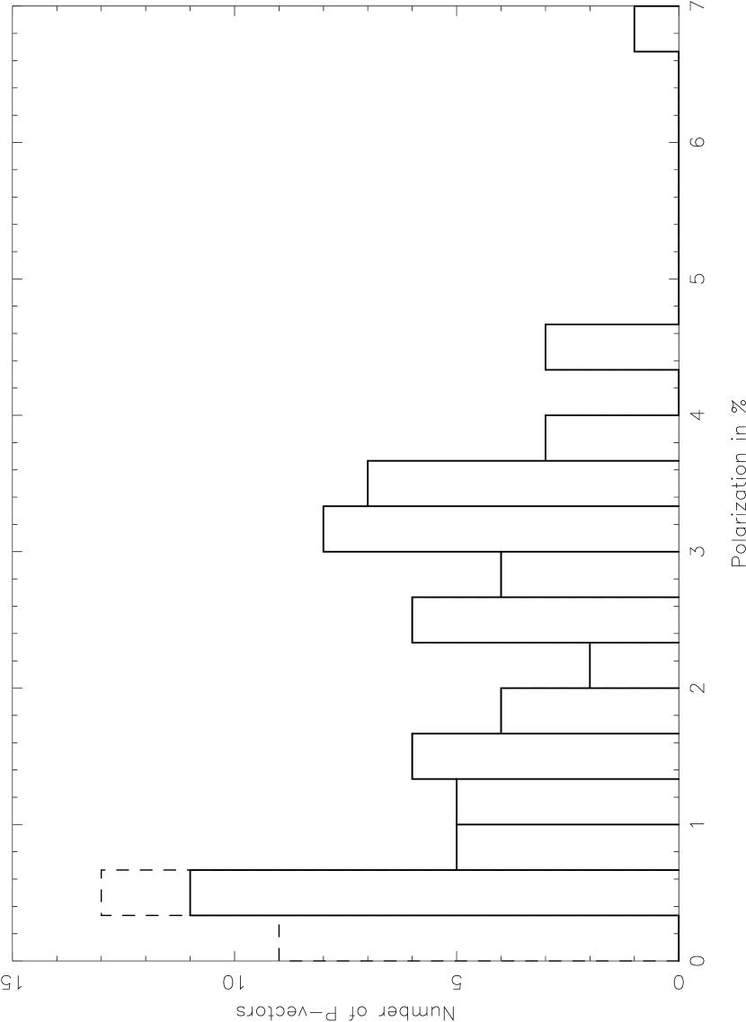
Figure 3: Histogram of polarization in GF 9. Data for which $P>3\sigma_{P}$ (See last column in Table 1) are shown with bold lines. For this set of data, the mean and the dispersion of the distribution of the degrees of polarization are $\overline{P}=2.22\%$ and $S_{\rm P}=1.33\%$ respectively.

Figure 2 presents a polarization map of stars for which the polarization degree meets the condition $P>3\sigma_{\rm P}$. This map is to be compared to Figure 1. The histogram of the degree of polarization is shown in Figure 3. If we only consider data for which $P>3\sigma_{P}$ (data shown with full lines), the mean and the standard deviation of the distribution are $\overline{P}=2.22\%$ and $S_{P}=1.33\%$, respectively. The histogram of the position angles is shown in Figure 4. If we only consider data for which $\sigma_{\theta}<9.5^{\circ}$ (data shown with full lines), the mean position angle and the standard deviation of this well peaked distribution are $\overline{\theta}=127.4^{\circ}$ and $S_{\theta}=25.5^{\circ}$, respectively. This means a standard deviation of 0.445 rad, comparable to those found for clouds with embedded clusters (see Myers $\&$ Goodman 1991b).

Stars S35, S70, S75, S86 and S92 are identified on both maps in Figures 1 and 2. Stars S35 and S86 are suspected to have variable linear polarization. These stars are located in the continuity of two filaments but in gaps where extinction appears to be relatively low. The data relative to these stars are compiled in Table 2 with the respective Julian Date (J.D.) of each measurement appearing in the last column.

The position angle of stars S70, S75 and S92 differ significantly from the mean direction of the other stars ($\overline{\theta}=127.4^{\circ}$ with $S_{\theta}=25.5^{\circ}$). Star S70 is a visual binary whose components fit both in the aperture hole used for the observations; its position angle is perpendicular to this mean position angle. Thus, we may be in the presence of a physical binary system with circumstellar material, or of a single system presenting intrinsic polarization and a background star. The difference of the position angles of stars S75 and S92 with the average value may be related to their position relative to the clouds as seen on Figure 1. Star S75 ($A_{V}=3.3$) is located north-east of IRAS 20520-6003 at the edge of two filamentary structures mainly parallel. Comparatively, star S92 is also located in a dense region ($A_{V}=2.1$) in a small filamentary structure oriented mostly north-south. Given their large extinction, these two sources could either be deeply embedded in their clouds or be young stellar objects surrounded with disks in which multiple scattering can produce a relatively high degree of polarization (e.g., Bastien & Ménard (1990)). Without multiwavelength data it is difficult to distinguish between these possibilities.

Three stars in our sample, GF 9 S1, GF 9 S2 and GF 9 S15 have measured spectral types and visual magnitudes. However we could not get reliable distances from these values. The $A_{V}$ values obtained are negative or yield very large distances. Similarly using $A_{V}$ values from Dobashi et al. (2005), we could not get reliable distances.

3.3 Variations of $P$ with A_V

In order to study the variations of the degree of polarization with visible extinction, we used the Dobashi et al. (2005) catalog to determine $A_{\rm V}$, in the direction of each star for which polarization measurements are available. This catalog is the first version of the atlas and catalog of dark clouds derived by using the optical database Digitized Sky Survey I (DSS), and applying a traditional star-count technique to 1043 plates contained in the DSS. Using the visible extinction coefficient $A_{\rm V}$ listed in Table 1, values of $P(\lambda=7660{\rm\AA})$ against $E_{\rm{B-V}}$, where $E_{\rm{B-V}}=\frac{A_{V}}{3.1}$, are shown in Figure 5. For all stars, except GF 9 S35 and GF 9 S86 (suspected variables), data directly observed at this wavelength are shown with crosses. Assuming NIR data from Jones (2003) and visible data probe the same types of grains, the Serkowski law,

$$P(\lambda)=P_{max}\rm{exp}[-Kln^{2}(\frac{\lambda_{\max}}{\lambda})],$$ (1)

where $\rm{K}=1.15$, is used to derive the relation $P_{\rm V}=1.97P_{\rm H}$. This relation is used to convert the H-band data to equivalent $\lambda=7660{\rm\AA}$ data, assuming $\lambda_{\rm max}=7660{\rm\AA}$. These equivalent data are listed in Table 3 and are shown with diamonds in Figure 5. As was previously mentionned by Jones (2003), no saturation of $P$ can be seen at about $A_{\rm V}\approx 1.3$ (or $E_{\rm{B-V}}\approx 0.4$), and $P_{\rm V}\approx 1.6\%$, as observed in cold dark clouds in Taurus (See Arce et al. (1998)). Data in the visible confirm this analysis but over the whole filament and the region surrounding it, and not just in the core region. Thus, while not universal, it is possible in some regions to probe magnetic fields inside dark clouds via polarimetry of background stars as suggested here by data taken in the visible and in the NIR.

4 Analysis and Discussion

4.1 Ambient Magnetic Field Orientation in the Vicinity of GF 9

As can be seen in Figure 2 and in the histogram of position angles in Figure 4, the polarization pattern in the vicinity of GF 9 is relatively well oriented on the plane of the sky with a mean direction of $\overline{\theta}=127.4^{\circ}$ and a standard deviation $S_{\theta}=25.5^{\circ}$. Since the filament has an incurved concentric shape reminiscent of supernova remnants (Schneider & Elmegreen (1979)), one can ask if a possible object at the origin of this shape could be located somewhere in the region delimited by the black circle traced in Figure 1. A possible candidate seems to be the post AGB star GLMP 1012 (see Figure 1) but given its distance estimate $d=$ 3 kpc (Preite-Martinez (1988)) compared with those of GF 9, even by considering $50$ km s^-1 winds, it is difficult to defend the view that this source can be responsible for the shape of the filaments. However since the problem is tridimensional, a source at the origin of such a shape could also be located outside of the domain defined by this circle. Maybe such a source exists but has not been detected, or the apparent concentric shape of the dense ISM is only a projection effect and other mechanisms, such as turbulent fluctuations in the ISM or density waves, are at the origin of its formation. A quick look in the catalogs reveals no potential candidate in a circle a few degrees in diameter around the position R.A.(2000) = 20${}^{\rm h}50^{\rm mn}53^{\rm s}$ and Dec.(2000) $=59^{\circ}51^{\prime}59^{\prime\prime}$.

If now one compares the direction of the inferred magnetic field with the orientation of the filamentary structures on the plane of the sky, it seems that the magnetic field has approximately the same orientation over an arc circle which covers about 135^o, from a position angle (P.A.) = 270^o to 45^o as measured from the center of the circle in Figure 1. When looking at both maps from east to west in Figure 1 and 2, a slow rotation of the direction of the field is present, the average directions near the core and near the filament regions differ by about 10^o (see Table 4), significantly under the variation in P.A. of the filament over the whole region. Moreover from east to west, there is a great dispersion in the orientation of the filamentary structures, thus it is hard with this two dimensional representation to see a direct impact of the field on the apparent shape of the filaments. This is in agreement with the fact that in other regions there is no prefered projected angle on the plane of the sky between the directions of the ambient magnetic field and the orientation of the filamentary structures (e.g. Myers & Goodman (1991b), Heyer et al. (1987)). See also Heiles et al. (2000) for a discussion on this subject.

4.2 Multiscale Analysis of the Magnetic Field

4.2.1 From filamentary clouds scale to cores scale

Comparisons of the orientation of the magnetic field according to the visible, IR and FIR data around and in the core and the filament regions can be done by looking at the maps in Figures 6 and 7 respectively. In the core region, when going from visible to IR, to FIR data, one can see an anticlockwise rotation of the P.A. by about 63^o in total. For each of these two regions, the means and dispersions of the degree of polarization and of the P.A. of the visible, IR and FIR data are compiled in Table 4. The P.A. for the FIR data corresponds to the observed polarization, rotated by 90^o to give the direction of the magnetic field. In Figures 6 and 7, only FIR data for which the P.A. is approximately the same when using the KLC instrumental polarization and the C-off instrumental polarization (Clemens 1999) are shown. The degree of polarization of the FIR data is not considered in the present analysis. Table 4 also includes similar information for the whole GF 9 region and for the local galactic scale, to be discussed below.

Comparison of Visible and IR data

First, visible and IR data do not probe the same regions on the plane of the sky. Visible data probe the more diffuse parts around prestellar cores while the IR data probe the denser phases where protostellar cores are present. Secondly we note that in the core region the IR vectors have approximately the same orientation which implies that the IR polarization is not intrinsic to each star but produced by dichroic absorption by aligned grains. This statistical argument, however, does not apply in the filament region where only one IR measurement with sufficient signal-to-noise ratio is available. Thirdly, in both cases the resolution used with each technique is comparable. Fourthly, the simple fact that the ‘IR’ magnetic field has not the same orientation than the ‘visible’ one implies that if the grains observed with these two techniques have identical properties, and if their dichroic absorption properties are the same at both IR and visible wavelengths, then the net polarization produced by aligned grains located in the densest parts of the cloud dominates the net polarization produced by aligned grains located in the foreground diffuse ISM. All these facts, in addition to the dependence of $P$ with $A_{\rm V}$ mentionned in section 3.3, suggest that there is a real rotation of the magnetic field lines in the core region when moving across the plane of the sky.

Comparison of IR and FIR data

Firstly, IR and FIR data probe the same regions on the plane of the sky in both the core and the filament regions. Secondly we note that in the core region the FIR vectors are very well aligned but not with the same P.A. than the IR vectors. IR data result from a magnetic field oriented at P.A. $\approx 171^{\circ}$ while FIR data suggest a magnetic field oriented at P.A. $\approx 19^{\circ}$. Thirdly, the resolution with these two techniques is not the same. The FIR data resolution is $\approx 80^{\prime\prime}$, many times the ‘pencil’ beam resolution of the IR and visible data. Finally, FIR observations probe the radiation emitted by grains mainly located in the densest parts of the cloud while IR observations probe grains located between the stars and the observer.

When looking at Figure 6, we see that IR and FIR data cover a common area $\approx 4^{\prime}\times 4^{\prime}$ in size. Thus if these two observational techniques probe the same column densities but at two different resolutions, one should be able to explain the rotation of the magnetic field lines as seen at these two wavelengths. A first hypothesis is that a given magnetic field morphology leads to several orientations according to the resolution at which it is observed (See Fiege & Pudritz (2000), but also Heitsch et al. (2001)). However, here we see that IR data are spatially distributed through FIR data, thus by using a simple principle of juxtaposition it seems impossible to reproduce the mean orientation of FIR vectors seen through $\approx 80^{\prime\prime}$ beams by combining several IR vectors with very small cross sections. On the other hand, since the mean position angle of the stars observed in the visible is not the same than the one for stars observed in the IR, these IR-observed stars should not be foreground to the clouds, but rather embedded in or background to the clouds. In what follows we review possible explanations for the shift in position angles.

(1) The stars observed in the IR could be located inside the GF 9 core. If this was the case, the impact of their presence on their immediate environment should be observed. IRAS observations of these stars show that their luminosities satisfy $L_{\rm submm}/L_{\rm bol}\sim 10\%$ (see section 2), which would argue against them being Class 0 sources, i.e., very young. Therefore, we reject the hypothesis that these IR stars are all embedded in the GF 9 core.

(2) The stars observed in the IR could be background to the GF 9 core region. This is suggested by their position in the $P-E_{\rm B-V}$ diagram shown in Figure 5. Two possibilities can be invoked to explain the difference in position angles:
(a) A first and may be naive approach is assume that grains along the line of sight to the GF 9 core are all at the same temperature, and that both the IR and FIR observational techniques probe all grains with the same efficiency. If this is right, the mean position angles observed at both wavelengths should be similar, except for the known 90⁰ difference between them. In this scenario, the difference in position angles is explained by a second cloud or filamentary structure located behind the GF 9 core, and in which dust grains would be aligned differently.
(b) A second and probably more realistic scenario is to emphasize differences related to the intrinsic nature of both observational techniques. Based on point (1) mentioned above, the assumption of a dust temperature gradient for an externally heated cloud seems reasonable. In this case, the FIR measurements should be more sensitive to “cold” dust grains aligned in the densest regions of the core than to “hot” dust grains aligned in the envelope and in the diffuse ISM. On the other hand, IR observations should probe all the grains along the line of sight, independently of their temperature. Thus grains aligned differently in the envelope than in the denser core should both contribute to the IR polarization position angle, explaining the offset in position angles.

While scenario (2b) does not reject the possibilty of a second cloud or filament evoked in (2a), it has the benefit to propose a simple and consistent explanation. Thus we prefer scenario (2b), in which the intermediate position angles of IR vectors shown in figure 6 may result from a vectorial addition of both FIR and visible vectors covering this region and its vicinity.

Comparisons of the magnetic fields orientations with the cores elongations

We compare in Table 5 the orientations of five protostellar cores spread into the filaments with the magnetic field orientations. Orientations of the cores L1082A, B and C were determined with the $(J,K)=(1,1)$ lines of NH₃ while orientations of the LM cores are based on the visible DSS data At first sight we see that, except for L1082B, these dark condensations have a tendency to be elongated along the filaments as was noticed by Myers et al. (1991a) (see Figures 1 and 2). Names, positions and P.A. of these cores are shown in Table 5 in columns 1 through 4 respectively. For objects LM351 and L1082C, located in the core region, and for objects LM349 and LM350, located in the filament region, the offset, $|\Delta\theta_{7660}|$, on the plane of the sky between the P.A. of each protostellar core and the mean magnetic field orientation probed with visible data is shown in column 5. The same is done with the IR and FIR measurements in columns 6 and 7 respectively. These offsets were not estimated for L1082B since the magnetic field direction is undersampled around this object.

On larger scales, the magnetic field is mostly along the minor axis of the cores, as can be seen in Figure 2. However, on smaller scales, if we accept that IR measurements can probe the magnetic field in dense regions as it is suggested by the variations of $P$ with $A_{V}$ shown in Figure 5, we see that a rotation of the field is apparent in the core region. On this smaller spatial scale the field is well aligned in the core region in a direction mainly parallel to the cores’ major axes. Turbulence models such as those developed by Padoan et al. (2001) show that matter may flow onto cores along filaments with the field being stretched along the filaments. In such a case, the field would tend to be along the major axis of the elongated low-density structures connected with higher density cores. However, such models show that the polarization pattern probing dust in the low density structures would be chaotic rather than smooth and well aligned. Moreover, Furuya et al. (2005) showed recently that a velocity gradient of 2.3 km s^-1 pc^-1 is present along the major axis of the core GF9-2 but none along its minor axis. Therefore, if we assume that sources named LM351, L1082C and GF 9-2 are associated to a common spatial volume traced with different tracers, and if we assume that the velocity gradient along the major axis of GF 9-2 is due to rotation of the core, this picture suggests that an original poloidal field has been twisted on small scales by the rotation of the core into a toroidal field. This would be consistent with a magnetic support model.

On the other hand, this effect does not seem to be present in the filament region where the magnetic field probed with IR data is mainly parallel to the small axes of the cores detected in this area, in approximately the same direction than the magnetic field seen at greater scales. But on the other hand if FIR measurements are reliable, the chaotic FIR polarization pattern suggests that turbulence plays an active role in the filament region.

Finally comparison of both regions suggests a magnetic field interacting differently, and maybe less with its surrounding medium in the filament than it does in the core region, in agreement with the evolutionary stage of these two regions. Additional IR data would be necessary to confirm this point, and the quality of FIR measurements should of course be confirmed in both regions.

4.2.2 From the filamentary clouds scale to the local Galactic scale

The mean orientation of the ambient magnetic field can also be compared to the local Galactic magnetic field orientation. Figure 8 shows a polarization map in Galactic coordinates based on measurements compiled by Heiles (2000) with data for which $P/\sigma_{P}>3$. The region presents a complicated picture because we are looking down a spiral arm and possibly because of the influence of the Cygnus star-forming complex. In their works Heiles (1996) and Walawender et al. (2001) have used a large set of polarization data and studied the inferred magnetic field geometry in this part of the Galaxy. At first sight, the simple picture of a toroidal magnetic field implies that the magnetic field lines should point in the direction toward $l=90^{\circ},b=0^{\circ}$. In their statistical study Walawender et al. (2001) show that this trend is effectively real and are also able to detect the curvature of the local spiral arm. As mentionned by Jones (2003), since GF 9 is at a relatively close distance it is probably threaded by the magnetic field in the local spiral arm. Jones compares the orientation of the mean IR vector in the core region with the visible vectors on a greater scale, and shows that this vector points in the direction of the ‘vanishing point’ approximately located at $l=90^{\circ},b=0^{\circ}$. We can see this vector denoted by ‘IR’ in Figure 8. We also show the mean visible vector ‘V’ in this map. It does not point in the same direction than the ‘IR’ vector but it is approximately parallel to its nearest neighbours. All these facts suggest that it is preferable to use data probing the diffuse parts of the ISM in the environments of molecular clouds to compare ambient to the cloud and Galactic magnetic field’s orientations.

4.3 Magnetic field strength and magnetic flux in the core region

In order to estimate if the core region observed in CS by Ciardi et al. (2000) is magnetically supercritical or magnetically subcritical, we use the Chandrasekhar & Fermi (1953) method to estimate the magnetic field strength. The magnetic field strength in the plane-of-sky is estimated with the expression:

$$B_{\rm pos}\approx 9.3\sqrt{n(\rm H_{2})}\frac{\Delta\rm(V)}{\delta\phi}\mu{\rm G},$$ (2)

where $\delta\phi$ is the polarization P.A. dispersion in degrees, $n(\rm H_{2})$ is the molecular hydrogen density in molecules cm^-3, $\Delta\rm V=\sqrt{8ln2}\delta\rm(V)$ is the FWHM line width in km s^-1, and $\delta\rm V$ is the velocity dispersion (see Crutcher (2004)).

We use only the IR data for the core region since we have no way of estimating the turbulent velocity dispersion for the larger area corresponding to the visible data. The value $\delta\phi=5.9^{\circ}$ is taken from Table 4 using the Jones IR data. This value is provided by a relatively small set of six measurements for which the mean of the uncertainties is $6.7^{\circ}$. If instead of a direct average, we use a weighted average for estimating the dispersion in P.A., we get $7.2^{\circ}$. Finally, working with the P.A. directly instead of the vectors, the dispersions are $6.4^{\circ}$ and $6.0^{\circ}$, weighted and unweighted respectively. All these values are close to each other and reflect the fact that there is little dispersion in P.A. in the cloud. Therefore, we believe that despite the small number of measurements, we nevertheless have a representative value for the dispersion. The various parameters that we used for the CS core region and our results are shown in Table 6.

Once $B_{\rm pos}$ is derived, we estimate $\lambda_{\rm obs}$, the observed mass to flux ratio $(\frac{M}{\phi_{B}})_{observed}$ normalized to its critical value. This observed normalized mass to flux ratio is subject to geometrical bias, as explained by Crutcher (2004). In the case of estimating the total field from the plane-of-sky component of the field, two of the three components are known and the correction factor for $\lambda_{\rm obs}$ is then $\pi/4$, which corresponds to $\lambda_{\rm c}$ given in Table 6. This correction is statistical in nature since we do not know the appropriate angle for any individual object. In fact, there may not be a line of sight component to the field. Using $\delta\phi=8.9^{\circ}$ for the dispersion in P.A. to take into account the uncertainties in the measurements would decrease the magnitude of $B_{\rm pos}$ and increase the magnitude of $\lambda_{\rm obs}$ and $\lambda_{c}$ by about 50%. For comparison, the dispersion in P.A. for the visible data around the core region is $12.4^{\circ}$ (Table 4). With this value (even though we are outside the area for which the CS line-widths have been measured), the values of $\lambda_{\rm obs}$ and $\lambda_{\rm c}$ are larger by about 110%. These values are probably too large because the visible data cover a much larger area than just the core region. Also, a bias exists in the Chandrasekhar-Fermi method that tends to cause estimated field strentghs to be too large and thus to underestimate values of $\lambda_{\rm obs}$ (e.g. Heitsch et al. (2001)).

What is the effect of the distance $d$ on these results? The column density $N$ is used to get the gas mass, so $M\propto r^{2}$, where $r$ is the radius of the cloud, assumed to be spherical. The density $n\propto M/volume\propto r^{-1}$. Since $r\propto d^{-1}$, $n\propto d$, $B_{pos}\propto d^{1/2}$ and $\lambda\propto d^{-1/2}$. If the distance is 200 pc instead of 440 pc as assumed for the values given in Table 6, $\lambda$ would be closer to unity by about $\sqrt{2}$.

Is there additional possible evidence for a subcritical core? Crutcher (2004) identified two other tests to distinguish between ambipolar diffusion and turbulence as supporting mechanisms for star formation. If ambipolar diffusion is acting, one would expect an hourglass configuration for the magnetic field. But the distribution of the IR polarization vectors (see Fig 6) suggests a smooth field, or even a slight curvature in the opposite direction than expected for an hourglass shape. A third test identified by Crutcher (2004), if ambipolar diffusion is acting one expects $B\propto\rho^{\kappa}$ with $\kappa$ approaching 1/2 for larger densitites ($\gtrsim 100$ cm^-3). The values derived here are more or less compatible with this relation (see Figure 1 in Crutcher (1999)). In addition, the comparison of the magnetic field orientations with the elongations of the cores seen in Table 5 is not in general compatible with ambipolar diffusion, since in that case the cores would be perpendicular to the direction of the magnetic field.

Taking all the above arguments into account, our data suggest that the GF 9 core region is approximately magnetically critical. Ambipolar diffusion does not appear to be supported. Also, turbulence would produce a randomness in the polarization vectors which is not observed. The picture presented in section 4.2.1 of an original poloidal field which is transformed into a toroidal field by rotation appears most plausible.

5 Conclusions

Visible linear polarization data taken at the Mont-Mégantic Observatory on 78 stars in the vicinity of the dark filamentary cloud GF 9 were presented and compared with available NIR and FIR polarization data covering part of the same region. Our main conclusions are:

On a scale of a few times the mean radial dimension of the molecular clouds, the magnetic field is smooth and well-ordered, and appears to be ‘blind’ to the spatial distribution of the filaments.

On smaller scales in the core region, NIR polarimetry shows a rotation of the magnetic field lines when reaching into the denser parts.

There is no evidence for saturation of polarization as a function of extinction for both the visible and NIR data, suggesting that even in the denser regions the same grain properties and grain alignment mechanisms apply, and that the magnetic field is still being probed adequately there.

Finally, the magnetic field strength was estimated with the Chandrasekhar & Fermi (1953) method. The results would suggest that the core region is approximately magnetically critical.

All these facts put together suggest that in GF 9 the magnetic field changes direction with the spatial scale. The field differs by $35^{\circ}$ in the GF 9 core compared to the surrounding region. Ambipolar diffusion does not appear to be supported given the current evidence. The effects expected from turbulence are definitely missing. A global interpretation of the results is that an original poloidal field could have been twisted into a toroidal configuration by a rotating elongated structure during its collapse.

Future work should check if the trend in polarization position angles to rotate counterclockwise with increasing wavelength still continues in the submm. Also, as the lack of saturation of polarization as a function of extinction suggests, if dust grains are magnetically aligned there should be no polarization hole in the submm in the core and the filament regions. As an additional benefit, submm polarization would afford a higher spatial resolution than the FIR data discussed here.

We thank the Conseil de recherche en sciences naturelles et en génie du Canada for supporting this research. The authors thank J. S. Greaves for providing information about observations of GF 9 with SCUBAPOL at the JCMT, as well as B. Malenfant and G. Turcotte for their helpful and friendly support during observations at Mont-Mégantic Observatory. We also thank an anonymous referee for his constructive comments and helpful suggestions. This work made extensive use of the SIMBAD database at the Canadian Astronomy Data Center, which is operated by the Dominion Astrophysical Observatory for the National Research Council’s Herzberg Institute of Astrophysics.

Table 1: Visible polarization data.

GSC	GF9	$\alpha(2000)$	$\delta(2000)$	$P\pm\sigma_{P}$	$\theta\pm\sigma_{\theta}$	AV	$\frac{P}{\sigma_{P}}>3$
number	number	(h mn s)	(∘ ’ ”)	($\%$)	(∘)	(Mag.)
no	91	20:47:23.5	+60:12:59.5	0.55$\pm$0.18	136.1$\pm$9.4	1.61	1
0424600447	40	20:47:25.8	+60:17:41.2	3.43$\pm$0.13	121.6$\pm$1.0	1.34	1
no	120	20:47:34.0	+59:51:54.4	4.36$\pm$0.29	113.7$\pm$1.9	2.09	1
0424601275	46	20:47:35.4	+60:03:35.1	0.24$\pm$0.12	87.1$\pm$13.8	1.89	0
no	92	20:47:47.6	+60:01:02.2	6.75$\pm$0.29	179.8$\pm$1.2	2.14	1
0424601151	57	20:47:48.0	+60:06:49.4	3.99$\pm$0.13	106.7$\pm$0.9	1.78	1
0424600411	31	20:47:50.2	+60:14:40.6	3.56$\pm$0.11	120.2$\pm$0.9	1.39	1
0396300254	48	20:48:01.0	+59:57:01.1	1.99$\pm$0.12	139.0$\pm$1.7	1.89	1
no	98	20:48:01.1	+60:00:47.1	0.41$\pm$0.26	79.9$\pm$18.1	2.13	0
0424600967	47	20:48:08.4	+60:00:24.6	2.63$\pm$0.13	124.4$\pm$1.4	1.66	1
0424600359	39	20:48:11.5	+60:18:52.2	3.21$\pm$0.11	115.4$\pm$1.0	1.14	1
0424601339	36	20:48:17.9	+60:06:26.9	0.68$\pm$0.13	138.2$\pm$5.5	2.22	1
0424600585	18	20:48:20.5	+60:01:15.2	0.70$\pm$0.10	135.3$\pm$4.1	1.66	1
0424600629	17	20:48:25.5	+60:10:11.9	0.06$\pm$0.09	37.3$\pm$49.6	1.97	0
0424600469	11	20:48:27.7	+60:32:54.5	0.82$\pm$0.11	128.1$\pm$3.9	0.64	1
0424601143	13	20:48:30.0	+60:24:59.4	1.08$\pm$0.09	115.2$\pm$2.4	0.98	1
0424601171	16	20:48:32.5	+60:15:08.4	3.36$\pm$0.11	119.1$\pm$1.0	1.43	1
0424600521	10	20:48:40.8	+60:32:15.1	0.54$\pm$0.12	132.5$\pm$6.1	0.66	1
0424600727	35	20:48:44.2	+60:09:52.9	see Table 2		2.17
0424601053	34	20:48:46.5	+60:09:42.4	3.99$\pm$0.12	109.5$\pm$0.8	2.17	1
0424600659	54	20:48:47.1	+60:12:49.4	3.21$\pm$0.13	116.7$\pm$1.1	1.73	1
0424600961	37	20:48:47.3	+60:01:45.4	2.14$\pm$0.13	127.0$\pm$1.7	1.24	1
0424601093	53	20:48:51.3	+60:13:46.1	3.39$\pm$0.12	118.5$\pm$1.0	1.69	1
0424600621	15	20:48:51.4	+60:15:27.6	0.61$\pm$0.04	151.5$\pm$1.8	1.38	1
0424600109	14	20:49:03.7	+60:18:57.7	0.97$\pm$0.13	129.9$\pm$3.7	1.27	1
0424601169	52	20:49:07.1	+60:05:05.0	3.28$\pm$0.13	126.3$\pm$1.1	1.17	1
0424600721	55	20:49:09.6	+60:18:43.4	3.54$\pm$0.13	115.8$\pm$1.0	1.56	1
0424600857	9	20:49:13.6	+60:30:03.6	$1.40\pm$0.11	131.6$\pm$2.3	0.75	1
no	90	20:49:14.1	+60:12:44.5	4.42$\pm$0.59	108.4$\pm$3.8	2.19	1
0424600123	8	20:49:14.4	+60:29:21.0	2.70$\pm$ 0.12	130.0$\pm$1.3	0.80	1
0424601087	38	20:49:15.7	+60:16:26.1	0.56$\pm$0.13	155.2$\pm$6.3	1.97	1
0424600963	51	20:49:18.6	+60:05:50.6	3.18$\pm$0.12	124.6$\pm$1.1	1.17	1
0424600281	56	20:49:18.7	+60:20:20.9	3.52$\pm$0.10	120.6$\pm$0.8	1.42	1
0396300376	19	20:49:33.3	+59:56:54.5	0.50$\pm$0.11	149.4$\pm$6.4	0.82	1
0424600981	7	20:49:33.7	+60:27:11.5	1.24$\pm$0.13	117.9$\pm$2.9	0.85	1
0396300020	20	20:49:41.5	+59:56:15.7	0.61$\pm$0.11	135.6$\pm$5.3	0.82	1
0424601133	21	20:49:44.1	+60:03:12.3	2.44$\pm$0.11	129.6$\pm$1.3	0.84	1
0424601015	6	20:50:04.3	+60:24:04.9	0.35$\pm$0.09	117.0$\pm$7.6	1.35	1
0424601131	42	20:50:25.7	+60:24:15.8	3.44$\pm$0.11	123.6$\pm$0.9	1.56	1
0424601183	50	20:50:25.8	+60:10:52.6	2.75$\pm$0.11	139.3$\pm$1.2	1.04	1
0424601341	33	20:50:31.9	+60:13:00.4	2.77$\pm$0.12	139.7$\pm$1.2	1.49	1
0424601127	44	20:50:36.8	+60:26:15.6	1.25$\pm$0.12	123.6$\pm$2.7	1.06	1
0424601041	32	20:50:37.2	+60:15:38.6	0.27$\pm$0.12	156.0$\pm$12.2	1.84	0
no	86	20:50:45.3	+60:20:01.4	see Table 2		2.36
0424600477	41	20:50:46.3	+60:23:26.3	2.53$\pm$0.15	127.3$\pm$1.7	1.39	1
0396300338	22	20:50:48.3	+59:58:22.0	1.86$\pm$0.11	132.8$\pm$1.7	0.77	1
0396300620	23	20:50:56.2	+59:59:30.6	0.51$\pm$0.12	180$\pm$6.7	0.73	1
0424600655	29	20:51:07.8	+60:11:24.2	2.63$\pm$0.13	136.2$\pm$1.4	1.34	1
0424601145	27	20:51:11.2	+60:06:26.2	3.14$\pm$0.10	133.0$\pm$0.9	1.06	1
0424601213	28	20:51:12.6	+60:08:53.9	2.48$\pm$0.12	139.2$\pm$1.4	1.16	1
0424601111	4	20:51:12.8	+60:25:15.5	1.36$\pm$0.09	133.3$\pm$1.8	1.33	1
0424600103	5	20:51:16.2	+60:33:19.9	1.32$\pm$0.13	124.3$\pm$2.8	1.14	1
no	70	20:51:32.3	+60:41:41.3	3.15$\pm$0.28	28.4$\pm$2.6	1.02	1
0424701143	43	20:51:33.6	+60:25:05.5	1.42$\pm$0.10	136.4$\pm$2.0	1.44	1
0424701033	45	20:51:34.7	+60:14:03.5	0.42$\pm$0.12	133.3$\pm$8.1	2.07	1
0424701049	30	20:51:43.7	+60:11:50.0	0.23$\pm$0.11	52.2$\pm$13.9	1.59	0
0396300164	24	20:51:49.2	+59:54:15.5	0.09$\pm$0.10	73.0$\pm$32.4	1.01	0
0424701155	26	20:51:51.7	+60:05:31.0	3.23$\pm$0.11	130.1$\pm$1.0	1.13	1
0424701211	3	20:51:53.4	+60:25:18.5	0.68$\pm$0.09	176.8$\pm$3.5	1.36	1
no	85	20:51:55.4	+60:19:00.0	0.11$\pm$0.43	91.8$\pm$57.7	2.29	0
0424701127	2	20:51:57.1	+60:22:44.6	0.13$\pm$0.07	87.4$\pm$15.7	1.87	0
no	71	20:52:01.8	+60:38:13.2	0.61$\pm$0.17	123.8$\pm$8.2	1.13	1
0424701215	1	20:52:02.7	+60:22:27.9	0.11$\pm$0.08	90.7$\pm$20.9	1.87	0
0424701115	25	20:52:04.5	+60:03:55.6	2.29$\pm$0.11	132.7$\pm$1.4	1.11	1
0424701085	72	20:52:23.2	+60:32:48.4	1.76$\pm$0.16	123.2$\pm$2.7	1.36	1
no	75	20:53:25.7	+60:16:32.6	1.25$\pm$0.23	85.7$\pm$5.3	3.29	1
no	68	20:53:42.0	+60:24:07.8	3.86$\pm$0.17	171.6$\pm$1.3	2.39	1
no	66	20:53:52.0	+60:26:37.7	4.48$\pm$0.34	152.8$\pm$2.1	2.52	1
no	59	20:53:52.8	+60:35:44.6	3.06$\pm$0.22	125.9$\pm$2.1	1.45	1
no	74	20:53:55.6	60:15:51.6	0.38$\pm$0.17	158.9$\pm$12.6	3.20	0
no	69	20:53:55.7	+60:22:55.9	1.47$\pm$0.20	131.6$\pm$3.8	2.72	1
no	69bis	20:53:59.0	+60:22:50.0	1.47$\pm$0.26	139.4$\pm$5.1	2.72	1
no	61	20:54:01.3	+60:39:55.3	0.50$\pm$0.16	146$\pm$9.2	1.15	1
no	77	20:54:27.8	+60:11:16.5	2.85$\pm$0.17	129.4$\pm$1.7	1.93	1
no	65	20:54:28.8	+60:26:53.5	1.42$\pm$0.21	143$\pm$4.2	2.32	1
0424700062	62	20:54:31.3	+60:32:40.7	2.53$\pm$0.15	141.3$\pm$1.7	1.90	1
no	64	20:54:53.0	+60:29:35.7	0.30$\pm$0.18	102.7$\pm$17.2	2.28	0
0424700686	73	20:56:15.6	+60:17:41.9	1.89$\pm$0.15	139.3$\pm$2.2	1.94	1

Table 2: Stars with suspected variable polarization. Coordinates are given in Table 1.

GF9	$P\pm\sigma_{P}$	$\theta\pm\sigma_{\theta}$	J.D.
number	$(\%)$	(o)	(days)
35	2.75$\pm$0.12	135.8$\pm$1.3	2,452,054.64583
35	0.43$\pm$0.13	$163.2\pm$8.7	2,452,141.72222
86	10.70$\pm$0.41	131.3$\pm$1.1	2,452,830.75347
86	12.41$\pm$0.37	15.4$\pm$0.8	2,452,835.78125

Table 3: NIR polarization data of Jones (2003) and equivalent $\lambda=7660{\rm\AA}$ polarization data in the core and in the filament regions. Visible extinction coefficients are from Dobashi et al. (2005).

Star	$P_{\rm H}\pm\sigma_{P_{\rm H}}$	$P_{7660}\pm\sigma_{P_{7660}}$	$A_{\rm V}$
	$(\%)$	$(\%)$	(Mag.)
C1	1.9$\pm$0.6	$3.7\pm 1.2$	2.34
C2	1.4$\pm$0.3	$2.8\pm 0.8$	2.34
C3	4.2$\pm$1.0	$8.3\pm 2.0$	2.60
C4	1.7$\pm$0.3	$3.4\pm 0.8$	2.34
C5	4.0$\pm$0.9	$7.9\pm 1.8$	2.60
C6	2.7$\pm$0.6	$5.3\pm 1.2$	2.34
F2	1.9$\pm$0.4	$3.7\pm 0.8$	2.19

Table 4: Means and dispersions of polarization and position angles at various wavelengths and various scales (see figures 6, 7, 2 and 8 respectively).

	Core region	Filament region	GF 9 scale	Galactic scale
$\overline{P}_{7660,\rm V}\pm S_{{P_{7660,\rm V}}}$ ($\%$)	$2.17\pm 0.93$	$2.62\pm 1.27$	$2.22\pm 1.33$	$1.44\pm 1.26$
$\overline{\theta}_{7660,\rm V}\pm S_{{\theta_{7660,\rm V}}}$ (∘)	$136.0\pm 12.4$	$126.1\pm 13.1$	$127.4\pm 25.5$	$72.0\pm 43.3$
$\overline{P}_{\rm H}\pm S_{{P_{\rm H}}}$ ($\%$)	$2.65\pm 1.10$	$1.9\pm 0.4$
$\overline{\theta}_{\rm H}\pm S_{{\theta_{\rm H}}}$ (∘)	$171.2\pm 5.9$	$137.0\pm 6.0$
$\overline{P}_{\rm FIR}\pm S_{{P_{\rm FIR}}}$ ($\%$)	…	…
$\overline{\theta}_{\rm FIR}+90^{\circ}\pm S_{{\theta_{\rm FIR}}}$ (∘)	$\approx 19$	random

Table 5: Position angles of cores in GF 9 and offsets with the mean magnetic field position angles as measured in the three different passbands.

Core	$\alpha(2000)$	$\delta(2000)$	P.A.	$|\Delta\theta_{7660}|$	$|\Delta\theta_{\rm H}|$	$|\Delta\theta_{\rm FIR}|$	Location
name	(h mn ${}^{\rm s})$	(∘ ’ ”)	(∘)	(∘)	(∘)	(∘)
LM349	20 49 6.9	60 11 48	47	$\approx 72$	$\approx 90$	random	F
LM350	20 49 46.5	60 15 40	49	$\approx 70$	$\approx 88$	random	F
LM351	20 51 28.0	60 18 33	43	$\approx 91$	$\approx 51$	$\approx 24$	C
LM352	20 53 49.9	60 11 27	…	…	…	…	…
L1082C	20 51 27.4	60 19 00	7	$\approx 53$	$\approx 15$	$\approx 12$	C
L1082A	20 53 29.6	60 14 41	…	…	…	…	…
L1082B	20 53 50.3	60 09 47	48	?	?	?	…

Table 6: Magnetic field strength in CS cores.

Parameter	GF9 Core
$n$ (H2 cm-3)	15000 $\pm$ 3000
$N$ (H2 cm-2)	9.9 $10^{21}$
$R(pc)$	0.16
$M$ $(M_{\bigodot})$	$15\pm 3$
$T_{K}(K)$	$7.5\pm 0.5$
$\Delta\rm V$ ($km/s$)	0.88$\pm$ 0.20
$\delta\phi$ $(^{\circ})$	$5.9$
$B_{\rm pos}$ ($\mu G$)	170$\pm$56
$\lambda_{\rm obs}$	$\approx$ 0.44
$\lambda_{\rm c}$	0.35

Figure 2: Visible polarization map of GF 9. The C and F rectangles are the core and the filament regions observed by Ciardi et al. (1998), Ciardi et al. (2000). Stars S75 and S92 are embedded in the filament and have a polarization with a different orientation from the mean orientation of the ambient magnetic field. Object S70 is a visual binary. Crosses show the positions of stars S35 and S86 for which variable polarization is suspected (See Table 2). Only data for which $P>3\sigma_{P}$ are represented in the Figure. Bold vectors with sizes of $2\%$ show position angles of cores LM349, LM350, LM 351, L1082C and L1082B. (See Figure 1).

Figure 4: Histogram of position angles of polarization in GF 9. Data for which $P>3\sigma_{P}$ (meaning $\sigma_{\theta}<9.5^{\circ}$) are shown with bold lines. For this set of data, the mean and the dispersion of the distribution of the position angles are $\overline{\theta}=127.4^{\circ}$ and $S_{\theta}=25.5^{\circ}$ respectively.

Figure 5: Variations of $P$ with $E_{\rm{B-V}}$. $A_{\rm V}$ data from Dobashi et al. (2005) were used to compute $E_{\rm{B-V}}$. The full line delineates the upper envelope $P\leq 9.0E_{\rm{B-V}}$ (Serkowski et al. (1975)). A linear fit to the whole data set is shown by the dashed line and is given by $P\approx 4.3E_{\rm{B-V}}$. Dotted lines reproduce the truncation in the $(P,E_{\rm{B-V}})$ relation observed by Arce et al. (1998) in dark clouds in Taurus. X symbols: broadband red data from Observatoire du Mont-Mégantic. Diamonds: NIR data from Jones (2003) converted to red-equivalent data (see section 3.3).

Figure 6: Polarization map around and into the core (C) region observed by Ciardi et al. (1998), Ciardi et al. (2000). Bold vectors represent visible data. Thin vectors are IR data from Jones (2003) with $P=1.5\%$ for clarity. Vectors with intermediate size are ISO FIR-90^∘ rotated data from Clemens et al. (1999) with $P=2.5\%$ for clarity. Only FIR data for which the position angle is approximately the same when using the KLC intrumental polarization and the C-off instrumental polarization are shown.

Figure 7: Polarization map in the filament region. Same as in Figure 6, but around and into the filament (F) region observed by Ciardi et al. (1998), Ciardi et al. (2000).

Figure 8: Galactic polarization map around GF 9. Visible data from the Heiles catalog in a $30^{\circ}\times 30^{\circ}$ box centered at position $(l_{c}=95^{\circ},b_{c}=+10^{\circ})$ are shown. The IR symbol denotes the mean IR polarization of data taken in the GF9 core region by Jones (2003). The V symbol shows the mean visible polarization from our data in the vicinity of the core region.

References

- André et al. (2000) André, Ph.; Ward-Thompson, D. and Barsony, M. 2000, Protostars and Planets IV, p59
- Arce et al. (1998) Arce, H. G.; Goodman, A. A.; Bastien, P.; Manset, N. and Sumner, M. 1998, ApJ 499, L93
- Barnard (1927) Barnard, E. E. 1927, Atlas of Selected Regions in the Milky Way, Carnegie Institute of Washington
- Bastien & Ménard (1990) Bastien, P. and Ménard, F. 1990, ApJ 364, 232
- Benson & Myers (1989) Benson, P. J. Myers, P. C. 1989, ApJSS, 71, 89
- Chandrasekhar & Fermi (1953) Chandrasekhar, S. and Fermi, E. 1953, ApJ 118, 113
- Ciardi et al. (2000) Ciardi, D. R.; Woodward, C. E.; Clemens, D. P.; Harker, D. E. and Rudy, R. J. 2000, AJ 120, 393
- Ciardi et al. (1998) Ciardi, D. R.; Woodward, C. E.; Clemens, D. P.; Harker, D. E. and Rudy, R. J. 1998, AJ 116, 349
- Clemens et al. (1999) Clemens, D.; Kraemer, K. and Ciardi, D. 1999, Workshop on ISO Plarisaton Observations, Eds. R.J. Laureijs R. Siebenmorgen. ESA-SP 435, p.7
- Crutcher (2004) Crutcher, R. M. 2004, Astrophysics and Space Science, v. 292, Issue 1, p. 225
- Crutcher (1999) Crutcher, R. M. 1999, ApJ 520, 706
- Crutcher et al. (2004) Crutcher, R. M.; Nutter, D. J.; Ward-Thompson, D. and Kirk, J. M. 2004, ApJ 600, 279
- Dobashi et al. (2005) Dobashi, K.; Uehara, H.; Kandori, R.; Sakurai, T.; Kaiden, M.; Umemoto, T. and Sato, Fumio 2005, PASJ 57, SP1, 1
- Dobashi et al. (1994) Dobashi, K.; Bernard, J. P.; Yonekura, Y. and Fukui, Y. 1994, ApJSS 95, 419
- Fiege & Pudritz (2000) Fiege, D. J. and Pudritz, R. E. 2000, ApJ 544, 830
- Froebrich (2005) Froebrich, D. 2005, ApJS 156, Issue 2, pp. 169-177
- Furuya et al. (2003) Furuya, R. S.; Kitamura, Y; Wootten, A.; Claussen, M. J. and Kawabe, R. 2003, ApJSS, 144, 71
- Furuya et al. (2005) Furuya, R. S.; Kitamura, Y; Shinnaga, H. 2005, Poster presented at Protostars and Planets V, no 8087
- Goodman et al. (1993) Goodman, A. A.; Benson, P. J.; Fuller, G. A. and Myers, P. C. 1993, ApJ 406, 528
- Goodman et al. (1995) Goodman, A. A.; Jones, T. J.; Lada, E. A. and Myers, P. C. 1995, ApJ 448, 748
- Güsten (1994) Güsten, R. 1994, in The Cold Universe, eds. Th. Montmerle et al. (Editions Frontières: Gif-sur-Yvette), p.169
- Heiles et al. (2000) Heiles, C.; Goodman, A. A.; McKee, C. F. and Zweibel, E. G. 2000, Protostars and Planets IV, p279
- Heiles (2000) Heiles, C. 2000, AJ 199, 923
- Heiles (1996) Heiles, C. 1996, ApJ 462, 316
- Heitsch et al. (2001) Heitsch, F.; Zweibel, E. G.; Mac Low, M-M.; Li, P.; Norman, M. L., 2001, ApJ 561, 800
- Heyer et al. (1987) Heyer, M. H.; Vrba, F. J.; Snell, R. L.; Schloerb, F. P., Strom, S. E., Goldsmith, P. F. & Strom, K. M. 1987, ApJ 321, 855
- Hilton & Lahulla (1995) Hilton, J. Lahulla, J.F. 1995, AASS 113, 325
- Houde et al. (2002) Houde, M.; Bastien, P.; Dotson, J. L.; Dowell, C. D.; Hildebrand, R. H.; Peng, R.; Phillips, T. G.; Vaillancourt, J. E. and Yoshida, H. 2002, ApJ 569, 803
- Houde et al. (2000a) Houde, M.; Bastien, P.; Peng, R.; Phillips, T. G. and Yoshida, H. 2000a, ApJ 536, 857
- Houde et al. (2000b) Houde, M.; Peng, R.; Phillips, T. G.; Bastien, P. and Yoshida, H. 2000b, ApJ 537, 245
- Houde et al. (2001) Houde, M.; Phillips, Thomas G.; Bastien, P.; Peng, R. and Yoshida, H. 2001, ApJ 547, 311
- Houde et al. (2004) Houde, M.; Dowell, C. D.; Hildebrand, R. H.; Dotson, J. L.; Vaillancourt, J. E.; Phillips, T. G.; Peng, R. and Bastien, P. 2004, ApJ 604, 717
- Jones (2003) Jones, T. J. 2003, AJ, 125, 3208
- Lazarian (2003) Lazarian, A. 2003, JQSRT 79-80, 881-902
- Lee & Myers (1999) Lee, C. W. Myers, P. C. 1999, ApJSS 123, 233
- Lynds (1962) Lynds, B. D. 1962, ApJS 7, 1
- Manset & Bastien (1995) Manset, N. and Bastien, P. 1995, PASP 107, 483
- Matthews et al. (2001) Matthews, B. C.; Wilson, D. W. and Fiege, J. D. 2001, ApJ 562, 400
- Myers et al. (1991a) Myers, P. C., Fuller, G. A., Goodman, A. A., Benson, P. J. 1991a, ApJ, 376, 561
- Myers & Goodman (1991b) Myers, P. C. and Goodman, A. A. 1991b, ApJ 373, 509
- Padoan et al. (2001) Padoan, P.; Goodman, A. A.; Draine, B. T.; Juvela, M.; Nordlund, Å. and Rögnvaldsson, Ö. E. 2001, ApJ 559, 1005
- Preite-Martinez (1988) Preite-Martinez, A. 1988, AA 76, 317
- Scarrott et al. (1990) Scarrott, S. M.; Rolph, C. D.; Semple, D. P. 1990, In Galactic and Interstellar Magnetic Fields, IAU Symposium 140, edited by R. Beck and P. P. Kronberg (Kluwer, Dordrecht), p. 245
- Serkowski et al. (1975) Serkowski, K., Mathewson, D. L., Ford, V. L. 1975, ApJ vol. 196, p. 261-290.
- Schleuning (1998) Schleuning, D. A. 1998, ApJ 493, 811
- Schneider & Elmegreen (1979) Schneider, S. Elmegreen, B. G. 1979, ApJSS 41, 87
- Vallée et al. (2003) Vallée, J. P.; Greaves, J. S. and Fiege, J. D.2003, ApJ 588, 910
- Viotti (1969) Viotti, N. R. 1969, Mem. Soc. Astron. Italiana, 40, 75
- Walawender et al. (2001) Walawender, J. M., Zweibel, E. G. Heiles, C. 2001, BAAS, 198, 41.05
- Wiesemeyer (1998) Wiesemeyer, H. 1998, ASP Conf. Series, Vol. 132., 189
- Wiesemeyer (1997) Wiesemeyer, H. 1997. The spectral signature of accretion in low mass protostars. PhD dissertation, University of Bonn