Analytical Study of Diffusive Relativistic Shock Acceleration

Abstract

Particle acceleration in relativistic shocks is studied analytically in the test-particle, small-angle scattering limit, for an arbitrary velocity-angle diffusion function $D$. Accurate analytic expressions for the spectral index $s$ are derived using few ($2-6$) low-order moments of the shock-frame angular distribution. For isotropic diffusion, previous results are reproduced and justified. For anisotropic diffusion, $s$ is shown to be sensitive to $D$, particularly downstream and at certain angles, and a wide range of $s$ values is attainable. The analysis, confirmed numerically, can be used to test collisionless shock models and to observationally constrain $D$. For example, strongly forward- or backward-enhanced diffusion downstream is ruled out by GRB afterglow observations.

Diffusive (Fermi) shock acceleration (DSA) is believed to be the mechanism responsible for the production of non-thermal, high-energy distributions of charged particles in collisionless shocks in numerous, diverse astronomical systems FermiAcc . Particle acceleration is identified in both non-relativistic and relativistic shocks, examples of the latter including shocks in gamma-ray bursts (GRB’s, where shock Lorentz factors $\gamma\gtrsim 100$ are inferred) grb , jets of radio galaxies Jets , active galactic nuclei AGNjets and X-ray binaries (micro-quasars) microquasars .

Collisionless shocks in general, and the particle acceleration involved in particular, are mediated by electromagnetic (EM) waves, and are still not understood from first principles. No present analysis self-consistently calculates the generation of EM waves and the wave-plasma interactions. Instead, the particle distribution (PD) $f$ is usually evolved by adopting some Ansatz for the scattering mechanism (e.g. diffusion in velocity angle) and neglecting wave generation and shock modification by the accelerated particles (the ”test-particle” approximation). This phenomenological approach proved successful in accounting for non-relativistic shock observations. For such shocks, DSA predicts a (momentum $p$) power-law spectrum, $d^{3}f/dp^{3}\propto p^{-s}$, where $s$ is a function of the shock compression ratio $r$, $s=3r/(r-1)$ NonRelDSA . For strong shocks in an ideal gas of adiabatic index $\Gamma=5/3$, $s=r=4$ (i.e. $p^{2}d^{3}f/dp^{3}\propto p^{-2}$), in agreement with observations.

Analysis of GRB afterglow observations suggested that the ultra-relativistic shocks involved produce high-energy PD’s with $s=4.2\pm 0.2$ grb_s . This triggered a numerical study of test-particle DSA in such shocks, $s$ calculated for a wide range of $\gamma$, various equations of state, and several scattering mechanisms (Bednarz98, ; Kirk00, ; Achterberg01, , and references therein). For isotropic, small-angle scattering in the ultra-relativistic shock limit, where upstream (downstream) fluid velocities normalized to the speed of light $c$ approach $\beta_{u}=1$ ($\beta_{d}=1/3$), spectral indices $s_{0;ur}=4.22\pm 0.02$ were found Bednarz98 ; Kirk00 ; Achterberg01 , in accord with GRB observations.

DSA analysis is more complicated when the shock is relativistic, mainly because $f$ becomes anisotropic. Monte-Carlo simulations EarlyMonteCarlo ; Bednarz98 ; Achterberg01 and other numerical techniques NumericalStudiesA ; Kirk00 ; NumericalStudiesB have thus been applied to the problem. For isotropic, small-angle scattering, an approximate expression for the spectrum was found Keshet05 ,

$$s_{0}=(3\beta_{u}-2\beta_{u}\beta_{d}^{2}+\beta_{d}^{3})/(\beta_{u}-\beta_{d})\mbox{ ,}$$ (1)

and shown to agree with numerical results; in particular it yields $s_{0;ur}=38/9\simeq 4.22$. Although $s$ was calculated numerically for various scattering mechanisms NumericalVeriousDiffusion , little qualitative understanding of the dependence of $s$ upon the scattering Ansatz has emerged. This motivates an analytical study of DSA in relativistic shocks, which may facilitate/test future self-consistent shock models.

This letter presents the first rigorous, fully analytical study of DSA in relativistic shocks. The (common) assumptions made are (i) the test-particle approximation; (ii) small-angle scattering, given by some velocity-angle diffusion function $D$; and (iii) $D$ is separable into an angular part times a space/momentum-dependent part. For discussion and physical examples of $D$, see FermiAcc ; NumericalStudiesA ; Kirk00 . In the analysis, $N$ angular moments of $f$ are used (and higher moments neglected) to accurately calculate $s$ even for small $N$. The moments are generalized in order to accelerate the convergence with $N$ and to obtain $s$ and $f$ for arbitrary $D$. For isotropic diffusion, the analysis reproduces and justifies previous results such as Eq. (1), good results obtained even with $N=2$. For anisotropic diffusion, the dependence of $s$ upon $D$ is analyzed, and is numerically confirmed and complemented. It is shown that $D$ can be constrained using observations, e.g. in GRB afterglows. The analysis works equally well for arbitrarily large $\gamma$, for which numerical methods become exceedingly difficult. Here we outline the main steps of the derivation and present its primary implications; the full analysis is deferred to a detailed, future paper.

Formalism.— Consider an infinite shock front at $z=0$, with flow in the positive z direction. Relativistic particles with momentum $\mathbf{\tilde{p}}$ much higher than any characteristic momentum in the problem are assumed to diffuse in the direction of momentum, $\tilde{\mu}\equiv\cos(\mathbf{\tilde{p}}\cdot\mathbf{\hat{z}}/\tilde{p})$, according to some diffusion function (DF) $\tilde{D}_{\mu\mu}$. The steady-state PD then satisfies the stationary transport equation NumericalStudiesA

$$\gamma_{i}(\beta_{i}+\tilde{\mu}_{i})\frac{\partial f(\tilde{\mu}_{i},\tilde{p}_{i},z)}{\partial z}=\frac{\partial}{\partial\tilde{\mu}_{i}}\left[\widetilde{D}_{\mu\mu}^{(i)}(\tilde{\mu}_{i},\tilde{p}_{i},z)\frac{\partial f}{\partial\tilde{\mu}_{i}}\right]\mbox{ ,}$$ (2)

where $\gamma=(1-\beta^{2})^{-1/2}$ is the fluid Lorentz factor and $i\in\{u,d\}$ are upstream/downstream indices, written henceforth only when necessary. Parameters are measured in the fluid frame (when marked by a tilde) or in the shock frame (otherwise), so the Lorentz invariant PD $f(\tilde{\mu},\tilde{p},z)$ is the density in a mixed-frame phase-space. The absence of a characteristic momentum scale implies that a power-law spectrum is formed, as verified numerically Bednarz98 ; Achterberg01 . With our assumption that $\widetilde{D}_{\mu\mu}$ is separable in the form $\widetilde{D}_{1}(\tilde{\mu})\widetilde{D}_{2}(\tilde{p},z)$, we may thus write Eq. (2) as

$$(\beta+\tilde{\mu})\partial_{\tilde{\tau}}q(\tilde{\mu},\tilde{\tau})=\partial_{\tilde{\mu}}[(1-\tilde{\mu}^{2})\widetilde{D}(\tilde{\mu})\partial_{\tilde{\mu}}\tilde{q}]\mbox{ ,}$$ (3)

where $f(\tilde{\mu},\tilde{p},z)\equiv\tilde{q}(\tilde{\mu},\tilde{\tau})\tilde{p}^{-s}$, and the spatial dimension was rescaled as $\tilde{\tau}\equiv\gamma^{-1}\int_{0}^{z}\widetilde{D}_{2}(\tilde{p},\check{z})d\check{z}$. The reduced DF $\widetilde{D}(\tilde{\mu})\equiv\widetilde{D}_{1}(\tilde{\mu})/(1-\tilde{\mu}^{2})$ is constant for isotropic diffusion.

Continuity across the shock front requires that $f_{u}(\tilde{\mu}_{u},\tilde{p}_{u},z=0)=f_{d}(\tilde{\mu}_{d},\tilde{p}_{d},z=0)$, where upstream and downstream quantities are related by a Lorentz boost of velocity $c(\beta_{u}-\beta_{d})/(1-\beta_{u}\beta_{d})$. Absence of accelerated particles far upstream and their diffusion far downstream imply that $f_{u}(z\to-\infty)=0$ and $f_{d}(\tilde{\mu}_{d},\tilde{p}_{d},z\to+\infty)=\tilde{f}_{\infty}\cdot\tilde{p}_{d}^{-s}$, where $\tilde{f}_{\infty}>0$ is constant (isotropic PD). Eq. (3) has been solved numerically under the above boundary conditions for specific choices of $\tilde{D}(\mu)$ Kirk00 .

Angular Moments.— In the shock frame, only a small fraction of the particles travel nearly parallel to the flow ($\mu\simeq\pm 1$), unlike the upstream frame where a substantial part of $f$ is beamed into a narrow, $\tilde{\mu}_{u}<-1+\gamma_{u}^{-1}$ cone. Angular moments of the shock-frame PD, $\int_{-1}^{1}\mu^{n}f\,d\mu$, thus diminish as $n\geq 0$ increases, suggesting that the problem can be approximately formulated using a finite number of low-$n$ moments. Next, we derive and solve equations for the spatial behavior of these moments; the boundary conditions are then used to determine $s$.

We work in the shock frame and use only shock frame variables henceforth, incorporating the Lorentz boosts into the transport equations. Writing Eq. (3) in the shock frame, using $p=\tilde{\gamma_{i}}\tilde{p}_{i}(1+\beta_{i}\tilde{\mu}_{i})$ and $\mu=(\tilde{\mu}_{i}+\beta_{i})/(1+\beta_{i}\tilde{\mu}_{i})$, we find that on each side of the shock

$$\mu\,\partial_{\tau}q(\mu,\tau)=\frac{\partial_{\mu}\left\{(1-\mu^{2})D(\mu)\partial_{\mu}\left[(1-\beta\mu)^{s}q\right]\right\}}{(1-\beta\mu)^{s-3}}\mbox{ ,}$$ (4)

where we defined $q(\mu,\tau)p^{-s}\equiv\tilde{q}(\tilde{\mu},\tilde{\tau})\tilde{p}^{-s}$, $D(\mu)\equiv\widetilde{D}(\tilde{\mu})$, and $\tau\equiv\gamma^{4}\tilde{\tau}$. An immediate consequence is that

$$\int_{-1}^{1}(1-\beta\mu)^{s-3}\mu\,q(\mu,\tau)d\mu=g=\mbox{const}\mbox{ ,}$$ (5)

where the boundary conditions yield $g_{u}=0$ and $g_{d}\propto\tilde{f}_{\infty}$. Eq. (5) is an expression of particle number and energy conservation in the fluid frame Keshet05 . A more general corollary of Eq. (4) is that for any function $h(\mu)$ for which $h/\mu$ is finite and continuously differentiable,

$$\partial_{\tau}\int_{-1}^{1}h(\mu)q(\mu,\tau)d\mu=\int_{-1}^{1}(1-\beta\mu)^{s}q$$ (6)

$$\times\partial_{\mu}\left\{\left(1-\mu^{2}\right)D(\mu)\partial_{\mu}\left[h(\mu)\mu^{-1}\left(1-\beta\mu\right)^{-(s-3)}\right]\right\}d\mu.$$

The spatial dependence of an angular moment $F_{n}(\tau)\equiv\int_{-1}^{1}\mu^{n}q(\mu,\tau)\,d\mu$ is given by Eq. (6) with $h=\mu^{n}$, if $n\geq 1$. Expanding the RHS integrand as a power series around $\mu=0$, we find that $\partial_{\tau}F_{n}$ is given by a linear combination of the moments $F_{a},F_{a+1}\ldots F_{b}$. Here, $a=\mbox{Max}\left\{0,n-3\right\}$, $b=n+2+n_{D}$, and $n_{D}$ is defined as the order of the power series of $D$ around $\mu=0$, $D(\mu)\propto 1+d_{1}\mu+d_{2}\mu^{2}+\cdots$, such that $n_{D}=0$ for isotropic diffusion. In matrix form, we may write

$$\partial_{\tau}\mathbf{F}(\tau)=\mathbf{A}\cdot\left(\begin{array}[]{c}F_{0}(\tau)\\ \mathbf{F}(\tau)\end{array}\right),$$ (7)

where $\mathbf{F}\equiv\left(F_{1},F_{2},\ldots\right)^{T}$. The (infinite) matrix $\mathbf{A}$ depends on $\beta$, $s$ and $D(\mu)$, so $\mathbf{A}_{u}\neq\mathbf{A}_{d}$. The boundary conditions imply that $\{F_{n}\}$ are continuous across the shock front $\tau=0$, vanish as $\tau\rightarrow-\infty$, and are finite for $\tau\rightarrow+\infty$. We show that a good, converging (in $N$) approximation to the solution is obtained using a small number $N+1$ of moments, $F_{0}\ldots F_{N}$, and neglecting higher order terms. This reduces $\mathbf{F}$ to an $N$-component vector and $\mathbf{A}$ to an $N\times(N+1)$ matrix.

The spatial dependence of the zero’th moment $F_{0}$ cannot be related to $n\geq 0$ angular moments through Eq. (6). This difficulty can be circumvented by adding an additional constraint to the system of equations. Expanding the integrand in Eq. (5) yields $\mathbf{G}(\beta,s)\cdot\mathbf{F}(\tau)=g$, or

$$F_{1}-(s-3)\beta F_{2}+\frac{1}{2}(s-3)(s-4)\beta^{2}F_{3}+\cdots=g\mbox{ ,}$$ (8)

independent of $D(\mu)$. Eq. (8) and its spatial derivative can be used to eliminate $F_{0}$ and $F_{N}$ from Eq. (7), giving an approximate, closed set of $\check{N}=N-1$ (or less, if $A$ is degenerate) ordinary differential equations (ODE’s),

$$\partial_{\tau}\mathbf{\check{F}}(\tau)=\mathbf{\check{A}}\cdot\mathbf{\check{F}}+g\mathbf{\check{G}}\mbox{ ,}$$ (9)

where $\mathbf{\check{F}}\equiv(F_{1},F_{2},\ldots,F_{\check{N}})^{T}$. Here, $\mathbf{\check{A}}\in M_{\check{N}}$ and $\mathbf{\check{G}}$ are functions of $\mathbf{A}$ and $\mathbf{G}$ obtained by combining Eqs. (7) and (8). For the relevant range of $s$, $\mathbf{\check{A}}$ is diagonalizable over $\mathcal{R}$. Thus, there exists a real matrix $\mathbf{P}\in M_{\check{N}}$, such that $(\mathbf{P}^{-1}\mathbf{\check{A}}\mathbf{P})_{mn}=\lambda_{n}\delta_{mn}$ and the eigenvalues $\{\lambda_{n}\}$ of $\mathbf{\check{A}}$ are real. The solution of Eq. (9) is then

$$F_{n}(\tau)=\sum_{m=1}^{\check{N}}\left[P_{nm}c_{m}e^{\lambda_{m}\tau}-gP_{nm}(\mathbf{P}^{-1}\mathbf{\check{G}})_{m}\lambda_{m}^{-1}\right].$$ (10)

The integration constants $c_{m,u}$ and $c_{m,d}$ along with $g_{d}$ and $s$ constitute $2\check{N}+1$ free parameters, as $\mathbf{F}$ is unique only up to an overall constant. The boundary conditions typically impose $2\check{N}+2$ constraints, so the problem is over-constrained. It is natural to relax the requirement that $F_{N}$ be continuous across the shock, as it is relatively small and $\partial_{\tau}F_{N}$ is relatively sensitive to neglected moments $n\gtrsim N$. The resulting discontinuity of $F_{N}$ at $\tau=0$ then provides an estimate of the approximation accuracy.

As an example, consider the simplest non-trivial approximation, where moments $F_{n}$ with $n>N=2$ are neglected. This is motivated, for example, by the suppression of $G_{n}$ [see Eq. (8)], $A_{1,n}$ and $A_{2,n}$ for $n>2$, if $s\simeq 4$. Here $\check{N}=1$, and the (single) ODE yields $F_{1}(\tau)=ce^{\lambda\tau}+g\check{G}\lambda^{-1}$. For isotropic diffusion, $\lambda=6\beta-(s-2)(s-3)(s-4)\beta^{3}$. In most cases of interest (where $s<5$) $\lambda>0$, corresponding to exponential decay upstream and divergence downstream. Therefor, $c_{d}$ must vanish, so $f_{d}$ is uniform in this approximation. This gives a cubic equation for $s$, independent of $g_{d},c_{u}$,

$$(s-3)\beta_{u}=\left.\frac{F_{1}}{F_{2}}\right|_{\tau=0}=\beta_{d}+\frac{2(s-1)\beta_{d}}{2+(s-2)(s-3)\beta_{d}^{2}}\mbox{ .}$$ (11)

The real root of this equation, shown in Figure 1, already agrees with numerical results and with Eq. (1) at a $\sim 5\%$ level ; in particular it yields $s_{0;ur}=4.27$. However, in this simple approximation $F_{0}$ is not continuous across the shock front (it has a $\lesssim 20\%$ jump), $s$ does not depend on $D_{u}(\mu)$, and its dependence on $D_{d}(\mu)$ is inaccurate.

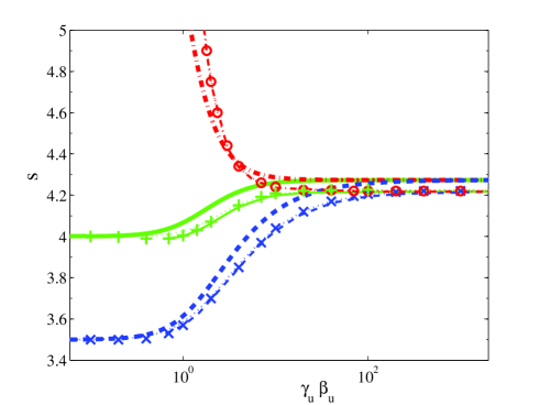
Figure 1: DSA for isotropic diffusion according to analytic approximations involving $F_{0}\ldots F_{2}$ [Eq. (11), heavy curves] or $L_{0}\ldots L_{5}$ (light curves), numerical calculations (Ref. (Kirk00, ), symbols) and Eq. (1) (dotted curves). Three types of strong shocks (see KirkDuffy99 ) are examined: using the Jüttner-Synge equation of state (solid curves/crosses), assuming a fixed adiabatic index $\Gamma=4/3$ (dashed curves/x-marks), and assuming a relativistic gas where $\beta_{u}\beta_{d}=1/3$ (dash-dotted curves/circles).

The convergence of the approximation with N depends on $D$, more moments required in general as $n_{D}$ and $|d_{n}|$ increase. Due to degeneracies in $\mathbf{A}$, $N=2,3,4,5,6,\ldots$ correspond to $\check{N}=1,1,2,3,3,\ldots$, and $N\geq 6$ is required in order to improve the $N=2$ approximation, e.g. $s_{0;ur}(N=6)=4.24$. The convergence is significantly accelerated if the moments are properly generalized.

Generalized Moments.— The analysis can be generalized in many ways by exploiting the freedom in the definition of the angular moments. For example, if we define $F_{n}(\tau)\equiv\int_{-1}^{1}q(\mu,\tau)w_{n}(\mu)f_{n}(\mu)\,d\mu$, where $\{f_{n}\}$ is an orthonormal basis in the interval $-1\leq\mu\leq 1$ with weight functions $\{w_{n}\}$, then the moments $\{F_{n}\}$ are simply the expansion coefficients of $q$ in terms of the basis $\{f_{n}\}$, i.e. $q(\mu,\tau)=\Sigma_{n}F_{n}(\tau)f_{n}(\mu)$ . With this choice of $\{F_{n}\}$, the analysis provides direct information about the PD $f$. Additional constraints on $f$ (e.g. Keshet05, ) may thus be used to estimate/improve the accuracy of the approximation. The analysis is mostly unchanged; it remains analytically tractable as long as $\mathbf{A},\mathbf{G}$ can be determined analytically, although the analogue of Eq. (11) is in general no longer a polynomial, becoming a transcendental equation in $s$.

As an example, let $f_{n}(\mu)=[(2n+1)/2]^{1/2}P_{n}(\mu)$ and $w_{n}=1$, where $P_{n}(\mu)$ is the Legendre polynomial of order $n$. The moments $\{F_{n}\}$ thus equal the coefficients $\{L_{n}\}$ of the Legendre series of $q$. Here we cannot take $N=2$, because the corresponding eigenvalue $\lambda$ is negative. For $N=3,4,5,\ldots$ we find $\check{N}=2,3,4,\ldots$, with $\check{N}_{u}=1,2,2,\ldots$ ($\check{N}_{d}=1,1,2,\ldots)$ non-vanishing exponents upstream (downstream). The resulting spectrum for isotropic diffusion is accurate to $\sim 5\%$, $2\%,1\%,\ldots$; in particular $s_{0;ur}=4.16,4.21,4.22,\ldots$. These results illustrate the rapid convergence of the Legendre-based analysis. The method is equally applicable for arbitrarily high $\gamma$, whereas numerical methods become exceedingly difficult as the ultra-relativistic limit is approached.

Isotropic (anisotropic) diffusion results for $s$ with $N=5$ Legendre moments are shown in Figure 1 (Figure 2). For isotropic diffusion, previous results are reproduced, lending rigor support for Eq. (1). The lowest order moments converge quickly, giving a rough estimate of $q(\mu,\tau)$ as a sum of components exponentially decaying in $|\tau|$ and, in the downstream, also a uniform part. The analytically calculated $s,q$ compare favorably with numerical results, which we calculate in the eigenfunction method of Kirk00 .

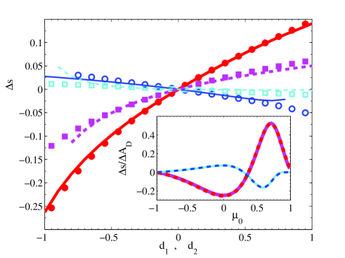
Figure 2: DSA for anisotropic diffusion. The spectrum is calculated numerically/with $L0\ldots L5$ (symbols/curves) for $D=1+d_{n}\mu^{n}$ in a $\gamma=10$, strong shock with the Jüttner-Synge equation of state. Plotted is $\Delta s=s-s_{0}$ vs. $d_{n}$ for $n=1$ (circles/solid curves) and $n=2$ (squares/dashed curves), downstream/upstream (filled/open symbols, heavy/light curves). Inset: local deviations from an isotropic DF down/upstream (heavy/light curves): $D=1+d_{0}\Theta(w_{0}-|\mu-\mu_{0}|)$ (solid curves) and $D=1+d_{0}\exp[-(\mu-\mu_{0})^{2}/2w_{0}^{2}]$ (dashed curves), where $(d_{0},w_{0})=(0.1,0.05)$ and $\Theta$ is the Heaviside step function.

Anisotropic diffusion.— Qualitatively good results for $d_{n\leq 3}\neq 0$; $d_{n\geq 4}=0$ are already obtained with $N=3$ Legendre-based moments. More complicated forms of the DF, involving additional $d_{n}\neq 0$ terms, require progressively larger $N$. Figure 2 shows that large $\Delta s=s-s_{0}$ values can be obtained for anisotropic diffusion in relativistic shocks. The spectrum is more sensitive to $D_{d}$ than it is to $D_{u}$, by a factor of a few. It is more sensitive to $d_{1}$ than to $d_{2}$; $|\Delta s(D=1+d_{n}\mu^{n})|$ is roughly monotonically decreasing with $n$. A linear, forward- (backward-) enhanced downstream DF, $D_{d}=1+d_{1}\mu$, yields $s>4.3$ ($s<4.0$) in a $\gamma>10$ shock, if $d_{1}>0.6$ ($d_{1}<-0.85$). Some forward- (backward-) enhanced choices of $D$ lead to more extreme spectra, e.g. $s_{ur}>4.6$ ($s_{ur}<3.7$). Constraints on $D_{d}$ may thus be imposed using observations that rule out such $s$ values, e.g. in GRB afterglows.

In order to elucidate the role of $D$, we numerically calculate $s$ for small deviations $\Delta D$, localized around some angle $\mu_{0}$, from an otherwise isotropic DF. The parameter $\Delta s/\Delta A_{D}$, where $\Delta A_{D}\equiv\int_{-1}^{1}\Delta D\,d\mu$, depends only weakly on the exact form of such $\Delta D$. Figure 2 (inset) shows that $s$ is sensitive to $\mu_{0}$, especially downstream. In general, the spectrum hardens when $D_{d}$ is enhanced at $\mu<\mu_{c}\simeq 0.4$ or diminished at $\mu>\mu_{c}$, and vice versa. Angles for which $\mu<\mu_{c}$ ($\mu>\mu_{c}$) roughly correspond to negative (positive) flux in momentum space, $j_{\mu}\propto-D(\mu)(1-\mu^{2})\partial_{\mu}q$, qualitatively accounting for this behavior. One way to see this is to note that the spectrum hardens when the average fractional energy gain $f_{E}$ (of a particle crossing, say, to the downstream and returning upstream) or the return probability (to the upstream) $P_{ret}$ increase; $s=3+\ln(1/P_{ret})/\ln f_{E}$ Achterberg01 . For example, enhanced diffusion in angles where $j_{\mu}<0$ shifts $q_{d}$ towards the upstream, raising both $P_{ret}$ and $f_{E}$. The above trend is roughly reversed upstream, but $\Delta s$ is smaller there and more sensitive to details of $\Delta D_{u}$.

I thank E. Waxman and D. Vinković for fruitful discussions.

References

- (1) For reviews see R. Blandford & D. Eichler, Phys. Rep. 154, 1 (1987); M. A. Malkov. & L. O’C. Drury, Rep. Prog. Phys. 64, 429 (2001).
- (2) T. Piran, Phys. Rep. 333, 529 (2000); P. Mészáros, ARA&A 40, 137 (2002); E. Waxman, Lect. Notes Phys. 598, 393 (2003).
- (3) M. C. Begelman, M. J. Rees, & M. Sikora, Astrophys. J. 429, L57 (1994); L. Maraschi, in AGNs: from Central Engine to Host Galaxy, Eds. S. Collin, F. Combes & I. Shlosman. ASP, Conference Series, 290 275 (2003).
- (4) M. J. Rees, Nature 229, 312 (1971); M. C. Begelman, R. D. Blandford & M. J. Rees, Rev. Mod. Phys. 56, 255 (1984); R. A. Laing, in Astrophysical Jets, ed. D. Burgarella, M. Livio & C. P. O’Dea (Cambridge: Cambridge Univ. Press), 95 (1993).
- (5) For review see R. Fender, astro-ph/0303339 [in Compact Stellar X-Ray Sources, edited by W.H.G. Lewin and M. van der Klis (Cambridge University Press, Cambridge, to be published)].
- (6) G. F. Krymskii, Dokl. Akad. Nauk SSSR, 234, 1306 (1977); W. I. Axford, E. Leer & G. Skadron, Proc. 15th Int. Cosmic Ray Conf., Plovdiv (Budapest: Central Research Institute for Physics) 11, 132 (1977); A. R. Bell, Mon. Not. R. Astron. Soc. 182, 147 (1978); R. D. Blandford & J. Ostriker, Astrophys. J. 221, L29 (1978).
- (7) E. Waxman, Astrophys. J. 485, L5 (1997); D. L. Freedman & E. Waxman, Astrophys. J. 547, 922 (2001); I. Berger, S. R. Kulkarni & D. A. Frail, Astrophys. J. 590, 379 (2003).
- (8) J. Bednarz & M. Ostrowski, Phys. Rev. Lett. 80, 3911 (1998).
- (9) J. G. Kirk, A. W. Guthmann, Y. A. Gallant, & A. Achterberg, Phys. Rev. 542, 235 (2000).
- (10) A. Achterberg, Y. A. Gallant, J. G. Kirk, & A. W. Guthmann, Mon. Not. R. Astron. Soc. 328, 393 (2001).
- (11) K. R. Ballard, & A. F. Heavens, Mon. Not. R. Astron. Soc. 259, 89 (1992); M. Ostrowski, Mon. Not. R. Astron. Soc., 264, 248 (1993).
- (12) J. G. Kirk & P. Schneider, Astrophys. J. 315, 425 (1987); A. F. Heavens & L. O’C Drury, Mon. Not. R. Astron. Soc. 235, 997 (1988).
- (13) M. Vietri, Astrophys. J. 591, 954 (2003); P. Blasi & M. Vietri, Astrophys. J., 626, 877 (2005).
- (14) U. Keshet & E. Waxman, Phys. Rev. Lett. 94, 111102 (2005).
- (15) D. C. Ellison & G. P. Double, Astroparticle Phys., 18, 213 (2002); M. Lemoine & G. Pelletier, Astrophys. J. Lett., 589, L73 (2003); A. Meli & J. J. Quenby, Astroparticle Phys., 19, 649 (2003); J. Niemiec & M. Ostrowski, Astrophys. J., 610, 851 (2004); D. C. Ellison & G. P. Double, Astroparticle Phys., 22, 323 (2004); J. Bednarz, PASJ, 56, 923 (2004); M. Lemoine & B. Revenu, Mon. Not. R. Astron. Soc., 366, 635 (2006).
- (16) J. G. Kirk & P. Duffy, J. Phys. G: Nucl. Part. Phys. 25, R163 (1999).