Time-Dependent Ionization in Radiatively Cooling Gas

Abstract

We present new computations of the equilibrium and non-equilibrium cooling efficiencies and ionization states for low-density radiatively cooling gas containing cosmic abundances of the elements H, He, C, N, O, Ne, Mg, Si, S, and Fe. We present results for gas temperatures between $10^{4}$ and $10^{8}$ K, assuming dust-free and optically thin conditions, and no external radiation. For non-equilibrium cooling we solve the coupled time-dependent ionization and energy loss equations for a radiating gas cooling from an initially hot, $\gtrsim 5\times 10^{6}$ K, equilibrium state, down to $10^{4}$ K. We present results for heavy element compositions ranging from $10^{-3}$ to $2$ times the elemental abundances in the Sun. We consider gas cooling at constant density (isochoric) and at constant pressure (isobaric). We calculate the critical column densities and temperatures at which radiatively cooling clouds make the dynamical transition from isobaric to isochoric evolution. We construct ion ratio diagnostics for the temperature and metallicity in radiatively cooling gas. We provide numerical estimates for the maximal cloud column densities for which the gas remains optically thin to the cooling radiation. We present our computational results in convenient on-line figures and tables (see http://wise-obs.tau.ac.il/$\sim$orlyg/cooling/).

1. Introduction

The collisionally controlled ionization states and radiative cooling rates of hot ($10^{4}-10^{8}$ K) low-density “coronal” gas clouds are crucial quantities in the study of the diffuse interstellar and intergalactic medium, including hot gas in supernova remnants, the Galactic halo, active galactic nuclei, galaxy groups and clusters, and warm/hot “baryonic reservoirs” in intergalactic clouds and filaments. In this paper we present new computations of the equilibrium and non-equilibrium cooling efficiencies and ionization states for radiatively cooling gas clouds with temperatures between $10^{4}$ and $10^{8}$ K. Our main emphasis is on the non-equilibrium cooling and ionization states that occur when an initially hot gas cools radiatively below $\sim 5\times 10^{6}$ K. Below this temperature, cooling can become rapid compared to ion-electron recombination, and the gas at any temperature tends to remain “over-ionized” compared to gas in collisional ionization equilibrium (CIE). Because the energy losses below $\sim 10^{7}$ K are dominated by atomic and ionic line emissions from many species, the non-equilibrium cooling rates also differ (are suppressed for over-ionized gas) compared to equilibrium cooling. The “recombination lag” and departures from equilibrium depend on the abundances of the heavy elements, and we present results for compositions ranging from $10^{-3}$ to 2 times the elemental abundances in the Sun. We include H, He, C, N, O, Ne, Mg, Si, S, and Fe, and we calculate the ion fractions as functions of temperature, for both equilibrium and non-equilibrium cooling, for all ionization stages of these elements.

The non-equilibrium radiative cooling of hot ($>10^{4}$ K), highly-ionized gas, with emphasis on the associated time-dependent ionization of the metal ions, is a classical problem first investigated by Kafatos (1973), and subsequently by several authors including Shapiro & Moore (1976), Edgar & Chevalier (1986), Schmutzler & Tscharnuter (1993), Sutherland & Dopita (1993), and Smith et al. (1996). Time dependent cooling in colder ($T\lesssim 10^{4}$ K) neutral hydrogen gas was studied earlier by Bottcher et al. (1970), Jura & Dalgarno (1972), and Schwarz et al. (1972) (see also Dalgarno & McCray [1972]). These investigations demonstrated that below a few $10^{6}$ K recombination lags can indeed lead to significant departures from CIE states and the associated equilibrium cooling rates. Computations of hot gas cooling efficiencies and ionization states assuming CIE have been presented in many papers dating back to House (1964), Tucker & Gould (1966), Allen & Dupree (1969), Cox & Tucker (1969), Jordan (1969), followed by Raymond et al. (1976), Shull & van Steenberg (1982), Gaetz & Salpeter (1983), Arnaud & Rothenflug (1985), Boehringer & Hensler (1989), and more recently Sutherland & Dopita (1993), Landi & Landini (1999), and Benjamin et al. (2001).

In this paper we reexamine the fundamental problem of non-equilibrium ionization in a time-dependent radiatively cooling gas. We focus on the behavior for pure radiative cooling with no external sources of heat or photoionization. Recombination lags and non-equilibrium ionization also occur in an initially hot gas undergoing rapid expansion and adiabatic cooling (Breitschwerdt & Schmutzler 1994; 1999). We do not consider such dynamical effects here.

Our work is motivated by ultraviolet (UV) and X-ray metal absorption-line spectroscopy of hot gas in the Galactic halo (e.g., Sembach & Savage 1992; Spitzer 1996), including, more recently, in discrete ionized “high-velocity clouds” (Savage et al. 2002; Fox et al. 2004, 2005, Fox, Savage, & Wakker 2006, see also Sternberg, McKee, & Wolfire 2002; Gnat & Sternberg 2004; Maller & Bullock 2004). We are also motivated by recent Hubble Space Telescope (HST), Far Ultraviolet Spectroscopic Explorer (FUSE), Chandra, and XMM-Newton, detections and observations of hot gas around the Galaxy (Collins et al. 2005; Fang et al. 2006), and/or of gas that may be part of a 10⁵-10⁷ K “warm/hot intergalactic medium” (WHIM) (Tripp, Savage, & Jenkins 2000; Shull, Tumlinson, & Giroux 2003; Richter et al. 2004; Sembach et al. 2004; Soltan, Freyberg, & Hasinger 2005; Nicastro et al. 2005; Savage et al. 2005, Williams et al. 2006; see however Rasmussen et al. 2006). This includes the temperature range where departures from equilibrium cooling are expected to be important. An intergalactic shock heated WHIM is expected to be a major reservoir of baryons in the low redshift universe (Cen & Ostriker 1999; Davé et al. 2001; Furlanetto et al. 2005). Important ions for the detection of such gas include C IV, N V, O VI, O VII, O VIII, Si III, Si IV, Ne VIII, and Ne IX.

The early discussions of Kafatos (1973) and Shapiro & Moore (1976) focused on time-dependent isochoric (constant density) cooling at a single metallicity. Sutherland & Dopita (1993) calculated isobaric (constant pressure) cooling efficiencies for a range of metallicities, but presented limited results for the time-dependent ion-fractions, and did not consider isochoric cooling. Schmutzler & Tscharnuter (1993) considered isochoric cooling for a range of metallicities, and presented ion-fractions only for solar metallicity gas. They presented limited results for isobaric cooling. In our calculations, we use up-to-date atomic data, and we present complete results for the time-dependent ion fractions and cooling efficiencies, for both isochoric and isobaric evolutions, for a wide range of metallicities. Because of the “$PdV$” work, isobaric cooling is less rapid than isochoric cooling, so departures from equilibrium are somewhat smaller in the isobaric case.

We consider metallicities ranging from $10^{-3}$ to twice the solar abundances of the heavy elements. In our calculations we assume that any initial dust is rapidly destroyed (e.g. by thermal sputtering) on a time-scale that is short compared to the initial cooling rate (Smith et al. 1996), and we consider dust-free cooling at fixed gas-phase elemental abundances. The sensitivity of the cooling efficiencies to the metallicity was studied by Boehringer & Hensler (1989) for equilibrium cooling, and by Schmutzler & Tscharnuter (1993) and Sutherland and Dopita (1993) for non-equilibrium conditions as well. Time-dependent effects are enhanced (diminished) as the cooling efficiencies are increased (reduced) for larger (smaller) gas-phase abundances of the heavy elements. Thus, recombination lags are more significant as the metallicity is increased. For a low-density gas, the non-equilibrium ion fractions and cooling efficiencies are independent of the gas density or pressure, because the ratio of the cooling and recombination times is independent of density. The density scales out of the problem. If the gas is assumed to cool, at either constant density or constant pressure, from an initial equilibrium state at high temperature, the only remaining free parameter in the problem is the metallicity $Z$.

We present results for the optically thin limit in which reabsorption of diffuse “self-radiation” may be neglected. We verify previous findings that trapping of hydrogen and helium recombination radiation, in optically thick clouds has only a small effect on the cooling and resulting ionization states. We also provide estimates of the maximal cloud column densities for which reabsorption of radiation from the metals (lines and continua) may be neglected in computations of the gas cooling efficiencies. Elsewhere, we will consider the effects of external fields on the non-equilibrium evolution of radiatively cooling gas. The inclusion of such radiation will introduce a pressure/density dependence via the ratio of the photoionization and recombination times.

In a separate paper we will present computations of the integrated metal ion “cooling columns” produced in steady flows of cooling gas (e.g. Edgar & Chevalier 1986; Dopita & Sutherland 1996; Heckman et al. 2002) including the effects of “upstream” cooling radiation on the “downstream” ionization states. Such flows occur, for example, in the radiative (isobaric) cooling layers behind steady shock waves (Shull & McKee 1979; Draine & Mckee 1993).

The outline of our paper is as follows. In §2 we write down the basic equations that we solve in our computations, and we describe our numerical method. In §3 we discuss isochoric versus isobaric cooling, and we derive critical cloud column densities and temperatures at which the dynamical transition from isobaric to isochoric cooling occurs. In §4 we present our computations of the ionization states as functions of gas temperature, for both CIE and non-equilibrium cooling. For time-dependent ionization we present results for both isochoric and isobaric evolutions. In §5 we present our computations of the radiative cooling efficiencies. We compare the CIE and non-equilibrium cooling efficiencies, and determine the temperatures below which non-equilibrium effects become important for each assumed metallicity. In this paper we have generated a large number of figures and tables containing results for metallicities ranging from $10^{-3}$ to 2 times solar. Some of the figures and tables appear in the main text, and some are available as online data files. Our data sets can be used to construct ion density-ratio diagnostics for radiatively cooling gas for a wide range of conditions. As an example, in §6 we discuss the evolution of the density ratios C IV/O VI versus N V/O VI in radiatively cooling gas. We summarize in §7.

2. Basic Equations and Processes

We are interested in studying the evolving ionization states of radiatively cooling gas, which is initially heated to some high temperature $T_{0}\gtrsim 5\times 10^{6}$ K, and then cools from an initial (equilibrium) ionization state. In the absence of continued heating and ionization the ions recombine as the gas cools, and the overall ionization state decreases with time. If the gas cools faster than it recombines, non-equilibrium effects become significant, and the gas remains over-ionized throughout the cooling. Non-equilibrium ionization leads to a suppression of the cooling rates. We compute this coupled time-dependent evolution for clouds cooling at constant density or constant pressure, for a wide range of metallicities. Non-equilibrium effects are most important at high metallicity, where the cooling times are shortest.

2.1. Ionization

In our numerical computations we follow the time-dependent ionization of an optically thin “parcel” of cooling gas, given an initial ionization state at an initial temperature $T_{0}$. We consider all ionization stages of the elements H, He, C, N, O, Ne, Mg, Si, S, and Fe. The temperature-dependent ionization and recombination processes that we include are collisional ionization by thermal electrons (Voronov 1997), radiative recombination (Aldrovandi & Pequignot 1973; Shull & van Steenberg 1982; Landini & Monsignori Fossi 1990; Landini & Fossi 1991; Pequignot, Petitjean, & Boisson 1991; Arnaud & Raymond 1992; Verner et al. 1996), dielectronic recombination (Aldrovandi & Pequignot 1973; Arnaud & Raymond 1992; Badnell et al. 2003, Badnell 2006; Colgan et al. 2003, Colgan, Pindzola, & Badnell 2004, 2005; Zatsarinny et al. 2003, 2004a, 2004b, 2005a, 2005b, 2006; Altun et al. 2004, 2005, 2006; Mitnik & Badnell 2004), and neutralization and ionization by charge transfer reactions with hydrogen and helium atoms and ions (Kingdon & Ferland fits, based on Kingdon & Ferland 1996, Ferland et al. 1997, Clarke et al. 1998, Stancil et al. 1998; Arnaud & Rothenflug 1985). Our atomic data set is the up-to-date compilation used in the steady-state photoionization codes ION (Netzer et al. 2005; and private communication) and Cloudy (Ferland et al. 1998).

We assume that the gas is dust-free (see below) and exclude neutralization processes by dust grains. Our code can also account for photoionization by a steady or time-varying external radiation field. However, in the computations presented here we exclude such radiation.

The time-dependent equations for the ion abundance fractions, $x_{i}$, of element $m$ in ionization stage $i$ are,

$$\begin{array}[]{l}d{x_{i}}/dt=x_{i-1}~{}~{}[q_{i-1}n_{\rm e}+\Gamma_{i-1}+k^{\rm H}_{\uparrow i-1}n_{\rm H^{+}}\\ \;\;\;\;\;\;\;\;\;\;\;\;\;\;\;\;\;\;\;\;\;\;\;\;\;\;+k^{\rm He}_{\uparrow i-1}n_{\rm He^{+}}]\\ \;\;\;\;\;\;\;\;\;\;\;+x_{i+1}~{}~{}[\alpha_{i+1}n_{\rm e}+k^{\rm H}_{\downarrow i+1}n_{\rm H^{0}}+k^{\rm He}_{\downarrow i+1}n_{\rm He^{0}}]\\ \;\;\;\;\;\;\;\;\;\;\;-x_{i}~{}~{}[(q_{i}+\alpha_{i})n_{\rm e}+\Gamma_{i}+k^{\rm H}_{\downarrow i}n_{\rm H^{0}}+k^{\rm He}_{\downarrow i}n_{\rm He^{0}}\\ \;\;\;\;\;\;\;\;\;\;\;\;\;\;\;\;\;\;\;\;\;+k^{\rm H}_{\uparrow i}n_{\rm H^{+}}+k^{\rm He}_{\uparrow i}n_{\rm He^{+}}]\ \ \ .\end{array}$$ (1)

In this expression, $q_{i}$ and $\alpha_{i}$ are the rate coefficients for collisional ionization and recombination (radiative plus dielectronic), and $k^{\rm H}_{\downarrow i}$, $k^{\rm He}_{\downarrow i}$, $k^{\rm H}_{\uparrow i}$, and $k^{\rm He}_{\uparrow i}$ are the rate coefficients for charge transfer reactions with hydrogen and helium that lead to ionization or neutralization. The quantities $n_{\rm H^{0}}$, $n_{\rm H^{+}}$, $n_{\rm He^{0}}$, $n_{\rm He^{+}}$, and $n_{\rm e}$ are the particle densities (cm^-3) for neutral hydrogen, ionized hydrogen, neutral helium, singly ionized helium, and electrons, respectively. $\Gamma_{i}$ are the photoionization rates of ions $i$, due to externally incident radiation. Here, we set $\Gamma_{i}=0$.

For each element $m$, the ion fractions $x_{i}\equiv n_{i,m}/(n_{\rm H}A_{m})$ must at all times satisfy

$$\sum x_{i}=1$$ (2)

where $n_{i,m}$ is the density (cm^-3) of ions in ionization stage $i$ of element $m$, $n_{\rm H}$ is total density of hydrogen nuclei, and $A_{m}$ is the abundance of element $m$ relative to hydrogen. The sum is over all ionization stages of the element.

In our time-dependent code we can explicitly account for the effects of trapping of hydrogen and helium recombination radiation by switching appropriately from “case A” to “case B” recombination, depending on the total cloud column density and temperature. As we discuss in the Appendix, we find that such trapping has generally only a small effect on the ionization states of the metals in the radiatively cooling gas. We therefore present results assuming optically thin case A conditions throughout. We also neglect reabsorption of line and continuum radiation emitted by metals in the cooling gas. In the Appendix we provide computational estimates of the maximal column densities for which reabsorption of the cooling radiation may be ignored.

2.2. Cooling

The ionization equations (1) are coupled to an energy equation for the time-dependent heating and cooling, and resulting temperature variation. Here we are interested in clouds undergoing pure radiative cooling with no heat sources.

For an ideal gas, the gas pressure $P=Nk_{\rm B}T/V$, and the internal thermal energy $U=3/2~{}Nk_{\rm B}T$, where $T$ is the gas temperature, $V$ is the total volume, $N$ is the total number of particles in the system, and $k_{\rm B}$ is the Boltzmann constant. If $dQ$ is an amount of heat lost (or gained) by the thermal electron gas, then

$$dQ=dU+PdV=\left(\frac{3}{2}+s\right)(Nk_{\rm B}dT+k_{\rm B}TdN).$$ (3)

where

$$s=\left\{\begin{array}[]{lcl}0&,&{\rm isochoric~{}cooling,~{}~{}{\it dV=}\ 0}\\ 1&,&{\rm isobaric~{}cooling,~{}~{}{\it dP=}\ 0}\\ \end{array}\right.$$ (4)

For pure radiative cooling, with no heating, $dQ\equiv-n_{e}n_{H}\Lambda(T,x_{i},Z)Vdt$ where $\Lambda(T,x_{i},Z)$ is the electron cooling efficiency (erg s^-1 cm³), which depends on the gas temperature, the ionization state, and the total abundances of the heavy elements specified by the metallicity $Z$. The electron cooling efficiency includes the removal of electron kinetic energy via recombinations with ions, collisional ionizations, collisional excitations followed by prompt line emissions, and thermal bremsstrahlung. For the low density “coronal limit” that we consider, $\Lambda$ is independent of the gas density or pressure.

In equation (3) we do not include the ionization potential energies as part of the total internal energy (e.g. Schmutzler & Tscharnuter 1993) since $dQ$ refers to the heat lost by the thermal electrons. In our definition of $\Lambda$, therefore, the ionization potential energy that is released as recombination radiation does not appear. Only the kinetic energy of the recombining electrons contributes to the cooling efficiency. On the other hand, kinetic energy removed via collisional ionization is included in our $\Lambda$. If ionization potential energy is considered as part of the total internal energy, then collisional ionization does not lead to a net energy loss, since the kinetic energy removed is merely stored as potential energy. Either way of accounting for the energy losses leads to the same temperature versus time relation $T(t)$.

It follows from equation (3) that the gas temperature declines at a rate given by (e.g., Kafatos 1973),

$$\frac{dT}{dt}=-\frac{n_{\rm e}n_{\rm H}\Lambda(T,x_{i},Z)}{(3/2+s)nk_{\rm B}}-\frac{T}{N}\frac{dN}{dt}$$ (5)

where $n\equiv N/V$ is the total particle density of the gas. Because of the $PdV$ work, the temperature declines more slowly for isobaric ($s=1$) cooling compared to isochoric ($s=0$) cooling.

The second term in equation (5) reflects the relative change in the total number of particles in the system. At temperatures $\gtrsim 10^{4}$ K, where the hydrogen and helium remain ionized, the number of particles remains approximately constant and this term may be neglected. It plays a role at lower temperatures as the hydrogen recombines (Kafatos 1973). For a primordial helium abundance, $A_{\rm He}\equiv n_{\rm He}/n_{\rm H}=1/12$ (Ballantyne, Ferland, & Martin 2000), the temperature declines at a rate

$$\frac{dT}{dt}\simeq\frac{n\Lambda}{4.34\times(3/2+s)k_{\rm B}},$$ (6)

for gas in which the hydrogen and helium are fully ionized.

Equation (5) can also be expressed as (e.g., Shapiro & Moore 1976),

$$\frac{3}{2}\frac{dP}{dt}-\frac{5}{2}\frac{P}{\rho}\frac{d\rho}{dt}=-n_{\rm e}n_{\rm H}\Lambda(T,x_{i},Z)$$ (7)

where $\rho=\mu n$ is the mass density of the gas, and $\mu$ is the mean mass per particle. For hydrogen and helium fully ionized, and a primordial helium abundance, $\mu=16/27~{}m_{\rm H}$ where $m_{\rm H}$ is the proton mass.

Equations (1) and (5) imply that in the absence of external radiation ($\Gamma_{i}=0$) the derivatives of the ion fractions with respect to temperature, $dx_{i}/dT\equiv(dx_{i}/dT)(dT/dt)$, are independent of the gas density or pressure. Because collisional ionization, electron-ion recombination, hydrogen and helium charge-transfer reactions, and the gas cooling processes are all “two-body” interactions, with rates per unit volume proportional to $n^{2}$, the density dependence divides out. The solutions for the ion fractions as functions of the instantaneous gas temperature, $x_{i}(T)$, are therefore independent of the assumed gas density or pressure.

Given a set of non-equilibrium ion abundances, $x_{i}(T)$, and an assumed metallicity $Z$, we use the cooling functions included in Cloudy (version 06.02, Ferland et al. 1998) to calculate $\Lambda(T,x_{i},Z)$. We present results for $Z$ ranging from $10^{-3}$ to 2 times solar. For $Z=1$ we adopt the elemental abundances for C, N, O, Mg, Si, S, and Fe reported by Asplund et al. (2005a) for the photosphere of the Sun. An exception is Ne, for which we adopt the “enhanced” abundance recommended by Drake & Testa (2005). We list our assumed solar abundances in Table 1. In all computations we assume a primordial helium abundance $A_{\rm He}=1/12$, independent of $Z$. The elements we include are the dominant coolants over the entire temperature range we study. Cooling by other elements is negligible.

Table 1Solar Elemental Abundances

Element	Abundance
	(X/H)⊙
Carbon	$2.45\times 10^{-4}$
Nitrogen	$6.03\times 10^{-5}$
Oxygen	$4.57\times 10^{-4}$
Neon	$1.95\times 10^{-4}$
Magnesium	$3.39\times 10^{-5}$
Silicon	$3.24\times 10^{-5}$
Sulfur	$1.38\times 10^{-5}$
Iron	$2.82\times 10^{-5}$

Non-equilibrium effects become important when the cooling time

$$t_{{\rm c}}\equiv\frac{T}{|dT/dt|}\simeq\frac{4.34\times(3/2+s)k_{\rm B}T}{n\Lambda(T,x_{i},Z)}$$ (8)

becomes short compared to the recombination time for an ion $i$,

$$t_{{\rm r},i}\simeq\frac{1}{n\alpha_{i}^{\rm tot}}\ \ \ ,$$ (9)

where $\alpha_{i}^{\rm tot}$ is the total recombination coefficient at the temperature $T$. The ionization state remains close to “collisional ionization equilibrium” (CIE) when $t_{\rm c}/t_{\rm r,i}>>1$ for the most abundant ions at the given temperature. Non-equilibrium effects become significant when $t_{\rm c}/t_{\rm r,i}<1$.

Because different ions have different recombination times, the recombination-lag is not similar for all ions. Ions with longer recombination times, in particular the helium-like ions, may be expected to persist over a wider range of temperatures when out of equilibrium.

Crucially, the ratios $t_{\rm c}/t_{\rm r,i}$ are independent of the gas density or pressure, so that departures from CIE are independent of the assumed gas density or pressure, for both isochoric or isobaric cooling. However, because $t_{\rm c}$ is shorter for isochoric cooling, non-equilibrium effects may be expected to be somewhat more pronounced for isochoric cooling compared to isobaric cooling.

The primary, and essentially only, “free parameter” in the problem is the metallicity $Z$ of the gas, through its control of $\Lambda$ and the cooling time. A higher $Z$ leads to enhanced metal line cooling, and larger departures from CIE, and vice versa.

In our computations we assume that the gas is dust-free, and we do not consider cooling via gas-grain collisions, a process that can dominate the total cooling at high temperatures if a high dust mass can be maintained (Ostriker & Silk 1973, Draine 1981). The neglect of dust is appropriate when the dust sputtering destruction time scale, $t_{\rm s}$, is shorter than the initial cooling rate, $t_{\rm c}$, so that any initial dust is destroyed before appreciable gas cooling occurs. Here we rely on the computations of Smith et al. (1996) who found that $t_{\rm s}/t_{\rm c}<1$ for $T\gtrsim 3\times 10^{6}$ K (see their Fig. 7). In our calculations we consider gas cooling from initial temperatures greater than this, and we assume that the dust is instantaneously destroyed. The gas then evolves with constant gas-phase elemental abundances specified by the assumed initial metallicity $Z$.

2.3. Numerical Procedure

For the atomic elements that we include, equations (1) and (5) are a set of $103$ coupled ordinary differential equations (ODEs). In our numerical procedure we advance the isochoric solutions in small pressure steps $\Delta P=\varepsilon~{}P$ where $\varepsilon\lesssim 0.05$, and $P$ is the current pressure, associated with a temperature $T(P)$. For isobaric conditions, we advance the solutions in small density steps $\Delta\rho=\varepsilon~{}\rho$, where $\rho$ is the current mass density, associated with a temperature $T(\rho)$.

For any $T$ we compute the total cooling rate by passing the current (non-equilibrium) ionization fractions $x_{i}(T)$ to the Cloudy cooling functions. We then use equation (7) to compute the time interval $\Delta t$ associated with pressure change $\Delta P$ (or density change $\Delta\rho$). We then integrate equations (1) over the time interval $\Delta t$ using a Livermore ODE solver (Hindmarsh 1983). When integrating the ionization equations (1), we assume that over the time step $\Delta t$, the pressure (or density) evolves linearly with time. In the integrations, the estimated local errors on the fractional abundances were controlled so as to be smaller than $10^{-6}$, $10^{-5}$, and $10^{-4}$ for hydrogen, helium, and metal-ions, respectively.

The above procedure is repeated with the new values of the ionization fractions, $x_{i}(T+\Delta T)$, down to a minimum temperature $T_{\rm low}$. Here we set $T_{\rm low}=10^{4}$ K. We verify convergence by re-running the computation at higher resolution (smaller $\varepsilon$), and confirming that the resulting ionization and cooling rates as functions of time remain unaltered.

3. Isochoric Versus Isobaric Cooling

A gas cloud will cool isochorically (i.e., at constant mass-density and volume) when the cooling time as defined by equation (8) is short compared to the dynamical time

$$t_{d}\equiv\frac{D}{c_{s}}$$ (10)

where $D$ is the cloud diameter, and $c_{s}=\sqrt{k_{\rm B}T/\mu}$ is the sound speed. Cooling is isobaric (i.e., occurs at constant pressure and decreasing volume) when the cooling time is long compared to the dynamical time.

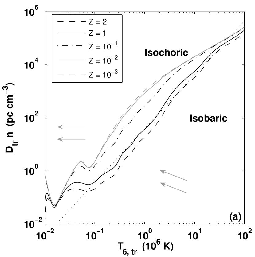
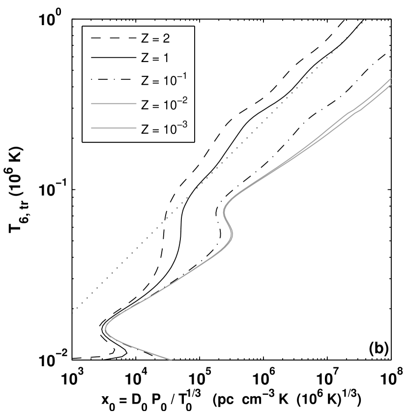
Figure 1.— Critical column densities, $D_{\rm tr}n$, and temperatures, $T_{\rm tr}$, for the transition from isobaric to isochoric cooling, for clouds with metallicities $Z$ ranging from $10^{-3}$ to $2$ times solar. (a) Transition column, $D_{\rm tr}n$, versus transition temperature, $T_{\rm tr}$, as given by equation (12). The dotted line is the power-law approximation for $Z=1$. In the region above the curves the cooling is isochoric. Below the curves the cooling is isobaric. The arrows indicate the direction in which the gas evolves as it cools. (b) Transition temperature, $T_{\rm tr}$, from isobaric to isochoric cooling, versus the initial state parameter $x_{0}\equiv D_{0}P_{0}/T_{0}^{1/3}$, as given by equation (13). The dotted line is the power-law approximation for $Z=1$.

The dynamical evolution is therefore determined by the ratio

$$\frac{t_{\rm c}}{t_{d}}\simeq 4.34\times\frac{(3/2+s)(k_{\rm B}T)^{3/2}}{\mu^{1/2}n\Lambda D}\ \ \ .$$ (11)

Cooling is isochoric when $t_{c}/t_{d}<<1$ and is isobaric when $t_{c}/t_{d}>>1$. Equation (11) shows that for a given cloud size and density the cooling is isobaric if the temperature is sufficiently high. This is because $T^{3/2}/\Lambda$ generally increases rapidly with increasing temperature (see §5). Conversely, for a given temperature and density, the cooling is isochoric for sufficiently large $D$.

For isochoric cooling, $D$ and $n$ remain constant with time. For these conditions $t_{\rm c}/t_{d}\propto T^{3/2}/\Lambda$, which generally decreases as the gas cools. Hence, cooling that is initially isochoric remains isochoric.

For isobaric cooling, a spherical cloud with initial diameter $D_{0}$, density $n_{0}$, and temperature $T_{0}$, will contract to a size $D=D_{0}(T/T_{0})^{1/3}$ with density $n=n_{0}T_{0}/T$ after cooling to a temperature $T$. Thus, as the cloud cools and contracts $t_{\rm c}/t_{d}\propto T^{13/6}/\Lambda$. This ratio decreases rapidly as the gas cools, so that a transition to isochoric cooling must eventually occur.

The transition from isobaric to isochoric cooling occurs at a critical cloud size, $D_{\rm tr}$, and temperature, $T_{\rm tr}$, at which $t_{\rm c}\simeq t_{d}$. It follows from equation (11) that the transition occurs at a critical column density

$$\begin{array}[]{l}D_{\rm tr}n\cong 10~{}k_{\rm B}^{3/2}\mu^{-1/2}\frac{T_{\rm tr}^{3/2}}{\Lambda(T_{\rm tr})}\\ \;\;\;\;\;\;\;\stackrel{{{}_{(Z=1)}}}{{\cong}}40\times T_{6,{\rm tr}}^{2.04}~{}{\rm pc}~{}{\rm cm}^{-3}\end{array}$$ (12)

where $n$ is the gas density. Given that non-equilibrium effects reduce the cooling efficiencies by only factors a few (see §5) compared to CIE cooling, we use the CIE cooling efficiencies, $\Lambda_{\rm eq}$, in equation (12) to estimate $D_{\rm tr}$ and $T_{\rm tr}$. The resulting estimates for the critical sizes and temperatures are then independent of initial conditions. For the numerical evaluation in equation (12) we use the power-law approximation $\Lambda_{\rm eq}^{Z=1}=2.3\times 10^{-19}~{}T^{-0.54}$ erg cm³ s^-1 for equilibrium cooling at solar metallicity (see §5).

For a cloud that initially cools isobarically at pressure $P_{0}$, from an initial diameter $D_{0}$ and temperature $T_{0}$, it then follows that

$$\begin{array}[]{l}\frac{D_{0}P_{0}}{T_{0}^{1/3}}\cong 10~{}k_{\rm B}^{5/2}~{}\mu^{-1/2}\frac{T_{\rm tr}^{13/6}}{\Lambda(t_{\rm tr})}\\ \;\;\;\;\;\;\;\stackrel{{{}_{(Z=1)}}}{{\cong}}4\times 10^{7}~{}T_{6,{\rm tr}}^{2.7}~{}\frac{{\rm pc}~{}({\rm cm}^{-3}~{}{\rm K})}{(10^{6}~{}{\rm K})^{1/3}}\end{array}$$ (13)

which provides an implicit relation for the temperature, $T_{\rm tr}$, at which the transition to isochoric cooling occurs (cf. Edgar & Chevalier 1986). The numerical evaluation is for the power-law cooling efficiency at solar metallicity.

In Figure 1 we plot $D_{\rm tr}n$ versus $T_{\rm tr}$ (left panel), and $T_{\rm tr}$ versus the parameter $x_{0}\equiv D_{0}P_{0}/T_{0}^{1/3}$ (right panel) as given by equations (12) and (13). We present results for metallicities $Z$ ranging from $10^{-3}$ to $2$ times solar, assuming the CIE cooling efficiencies we compute in §5.

In Figure 1a, the cooling for each $Z$ is isochoric for temperatures and cloud column densities to the left and above of the curves. The cooling is isobaric to the right and below the curves. The dotted line in Figure 1a is the power-law approximation given in equation (12). The arrows in Figure 1a indicate the direction in which the gas evolves as it cools. For isochoric cooling the column $Dn$ remains constant, and the gas cools along horizontal trajectories. For isobaric cooling $Dn\propto T^{-2/3}$, as indicated by the inclined arrows, showing that the gas must eventually make the transition to isochoric cooling. For example, a condensation with diameter $D=10$ kpc, density $n=10^{-5}$ cm³, and temperature $T=10^{6}$ K (corresponding to a thermal pressure $P=10$ cm^-3 K) cools isobarically, since $Dn=0.1$ pc cm^-3, whereas for this temperature $D_{\rm tr}n=40$ pc cm^-3 for $Z=1$, or $10^{3}$ pc cm^-3 for $Z<10^{-2}$.

In Figure 1b, $T_{\rm tr}$ is the temperature at which the transition from isobaric to isochoric cooling occurs, given an initial state defined by the parameter $x_{0}$. In computing $T_{\rm tr}$ we again use the equilibrium cooling efficiencies for the different values of $Z$. The dotted line in Figure 1b shows the power-law approximation for $Z=1$ as given in equation (13). For our above example (with $D=10$ kpc, $P=10$ cm³ K, $T=10^{6}$ K), the parameter $x_{0}=10^{5}$, so that the initial isobaric condensation will begin cooling isochorically at $T_{\rm tr}=10^{5}$ K for $Z=1$, or at $4\times 10^{4}$ K for $Z<10^{-2}$.

As we show in the Appendix, a cooling gas cloud remains optically thin up to column densities that are much greater than the critical transition columns in Figure 1. Expressions (12) and (13), and the curves in Figure 1 are therefore of broad applicability for determining the isobaric versus isochoric dynamical evolution for radiatively cooling clouds.

4. Ionization Fractions

We have carried out computations of the collisionally controlled ionization states of the elements H, He, C, N, O, Ne, Mg, Si, S, and Fe, as functions of gas temperature for three sets of assumptions. First we assume CIE imposed at all $T$. Then we consider the non-equilibrium ionization states as functions of the time-dependent temperature for radiatively cooling gas, for constant pressure and constant density evolutions. Our results are displayed in Figure 2 and listed in tabular form in Tables 2-4, and in additional tables and figures that we describe below.

The left-hand panels of Figure 2 show our results for the CIE ion fractions $x_{i}^{\rm eq}(T)$. Each panel displays the ionization stages of a particular element. In our CIE computations we have integrated the time-dependent equations (1) to the equilibrium states reached at late times when the formation and destruction rates for each ion are equal. We performed these time integrations at fixed temperatures $T$ ranging from 10⁴ to 10⁸ K. For purposes of comparison with our non-equilibrium computations, in Figure 2 we display results for temperatures between $10^{4}$ and $5\times 10^{6}$ K only. Results for higher temperatures, up to 10⁸ K where nearly all of the ions become fully stripped, are given in Table 2. We verified that the CIE solutions we obtained by time-integration are identical to those found by solving the set of algebraic equations for $x_{i}$ obtained by setting $dx_{i}/dt=0$ in equation (1), as appropriate for steady state.

Table 2CIE Ion Fractions

Temperature	H0/H	H+/H	He0/He	…
(K)
$1.00\times 10^{4}$	$9.99\times 10^{-1}$	$9.30\times 10^{-4}$	$1.00\times 10^{0}$	…
$1.05\times 10^{4}$	$9.97\times 10^{-1}$	$2.88\times 10^{-3}$	$1.00\times 10^{0}$	…
$1.10\times 10^{4}$	$9.93\times 10^{-1}$	$6.98\times 10^{-3}$	$1.00\times 10^{0}$	…
$1.15\times 10^{4}$	$9.84\times 10^{-1}$	$1.51\times 10^{-2}$	$1.00\times 10^{0}$	…
$1.20\times 10^{4}$	$9.69\times 10^{-1}$	$3.05\times 10^{-2}$	$1.00\times 10^{0}$	…

Note. — (1) The complete version of this table is in the electronic edition of the Journal. The printed edition contains only a sample. (2) CIE ion fractions are given for $Z=1$. For $T\lesssim 10^{4}$ K the electron density, and associated ion fractions, depend on $Z$.

For an ionized hydrogen gas, the CIE ion fractions are independent of the metallicity $Z$, and are “universal” functions of the gas temperature $T$, as determined by the microscopic steady-state balance between electron impact collisional ionization, electron-ion recombination, and charge transfer. Our CIE solutions, and in particular the shapes and peak positions of the $x_{i}^{\rm eq}(T)$ curves, are in excellent agreement with previous computations available in the literature (see §1). Our CIE ion fractions differ only slightly from the widely quoted results of Sutherland & Dopita (1993). For example, as found by Sutherland & Dopita for carbon (see their Fig. 3), $x({\rm C^{3+}})$ peaks at a value of $0.3$ around a narrow temperature range close to $10^{5}$ K, whereas $x({\rm C^{4+}})$ is close to 1 for a broad temperature range from $\sim 1.5\times 10^{5}$ K to $\sim 7\times 10^{5}$ K. The widths of the $x_{i}^{\rm eq}(T)$ curves reflect the magnitudes of the ionization potentials of the ions. For example, C⁴⁺, N⁵⁺, and O⁶⁺ persist for a wide range of temperatures due to the increase in thermal energy scale that is required to remove the inner K-shell electrons.

The right-hand panels of Figure 2 display our results for non-equilibrium ionization in radiatively cooling gas for solar ($Z=1$) composition. For time-dependent cooling the behavior depends on the initial conditions. Here we assume that the gas is cooling from an initially hot, $T>5\times 10^{6}$ K, equilibrium state. For such high temperatures the cooling times are long, and there is generally sufficient time for the gas to reach CIE before appreciable cooling occurs. Our results are also listed in “on-line” Tables 3 and 4. Results for other metallicities are presented in additional electronic on-line figures and tables. In each panel in Figure 2, the black curves are for isochoric cooling, and the light grey curves are for isobaric cooling. Departures from CIE become apparent for $T\lesssim 10^{6}$ K, for which cooling becomes rapid compared to recombination.

When departures from equilibrium occur, the gas at any temperature remains over-ionized compared to CIE, as recombination lags behind cooling. The recombination lag affects all elements including hydrogen and helium. For example, in CIE the hydrogen is half-ionized at $T=1.6\times 10^{4}$ K, and is fully neutral ($99.9\%$) at $10^{4}$ K. However, for non-equilibrium (isochoric) cooling for $Z=1$ the hydrogen is only $9\%$ neutral at $10^{4}$ K. The metals are affected in a similar manner, with $x_{i}(T)$ remaining overionized compared to CIE at low temperatures. The recombination lags are largest for ions with small recombination efficiencies. Thus, He-like ions, such as C⁴⁺, N⁵⁺, and O⁶⁺, which have long recombination times, persist to much lower temperatures in radiatively cooling gas compared to CIE. For example, for solar composition $x({\rm C^{4+}})>0.2$ down to $T\sim 1.4\times 10^{4}$ K for isochoric cooling, and $2.3\times 10^{5}$ K for isobaric cooling, whereas in CIE $x^{\rm eq}({\rm C^{4+}})$ becomes vanishingly small for $T$ below $\sim 8\times 10^{4}$ K. Similarly, the non-equilibrium abundance of the widely observed ion O⁵⁺ remains greater than 10% of its peak value of $0.11$ occurring at $3.0\times 10^{5}$ K, down to temperatures of $2.0\times 10^{4}$ K for isochoric cooling, and $1.0\times 10^{5}$ K for isobaric cooling. In CIE, O⁵⁺ vanishes below $\sim 2\times 10^{5}$ K.

Figure 2 shows that at high temperatures, where CIE is attained, the isobaric and isochoric $x_{i}(T)$ curves converge as they must. However, for lower temperatures, the recombination lags are greater for isochoric cooling compared to isobaric cooling. This is due to the shorter isochoric cooling times (see equation [8]). The isochoric and isobaric ion fractions differ most substantially for ions with the largest recombination lags. The differences grow with increasing metallicity as the cooling times become shorter.

Another important feature of the time-dependent ion distributions is the “double-peaked” behavior of the $x_{i}(T)$ curves seen for many ions, e.g. C⁺⁺, C³⁺, Si³⁺, S⁴⁺, and S⁵⁺. This behavior reflects the temperature dependence of dielectronic versus radiative recombination (Kafatos 1973). For such ions, dielectronic recombination is the dominant removal mechanism from the high-temperature peaks to the central minima. At lower temperatures dielectronic recombination weakens, and the ion fractions rise again due to continuing recombination from the persisting higher ionization stages. As the temperature continues to decrease, radiative recombination becomes increasingly effective and the ion fractions drop again, leading to the low-temperature peaks. The double-peaked behavior is a time-dependent effect, because the low-temperature peaks occur at temperatures for which the ions no longer exist in CIE.

Our non-equilibrium $x_{i}(T)$ curves are in qualitative agreement with previous computations (Kafatos 1973, Shapiro & Moore 1976, Sutherland and Dopita 1993, Schmutzler & Tscharnuter 1993). However, there are some significant differences in detail which are due, at least in part, to differences in the assumed atomic processes and rate coefficients. For example, the early studies by Kafatos (1973) and Shapiro & Moore (1976) did not include charge transfer reactions with hydrogen or helium, which affect the ion fractions for $T\lesssim 10^{5}$ K. Differences between our results and the more recent computations of Sutherland and Dopita (1993) and Schmutzler & Tscharnuter (1993) are likely due to differences in dielectronic rate coefficients (which control the “double-peak” behavior) and in the assumed solar abundances. For example, Sutherland & Dopita adopted the Anders & Grevesse (1989) abundances with ${\rm O/H}_{\odot}=8.5\times 10^{-4}$, whereas we adopt the more recent Asplund et al. (2005a) value of $4.6\times 10^{-4}$ (see Table 1). Different assumed abundances lead to altered cooling times and departures from CIE.

Our results for the non-equilibrium ion fractions, $x_{i}(T)$, for metallicities $Z$ equal to $10^{-3}$, $10^{-2}$, $10^{-1}$, and $2$, are presented in electronic “on-line” Figures 3-6, and Tables 5-12. Here we consider two examples of how the assumed metallicity affects the ion fractions. In Figure 7 we display the O⁵⁺ and O⁺⁺ distributions for the different values of $Z$ in isochorically cooling gas. At high temperatures ($\gtrsim 5\times 10^{6}$ K) the cooling times are long for all $Z$, and the O⁵⁺ and O⁺⁺ abundances converge to the CIE distributions (thick grey curves). Departures from CIE occur at lower temperatures. The departures are largest for large $Z$ where the cooling times are shortest. For example, for $Z=2$ the O⁵⁺ distribution is very broad, and this ion persists down to $\sim 10^{4}$ K, remaining within a factor $3$ of its peak abundance of $0.1$ at $T=1.7\times 10^{4}$ K. For smaller $Z$ the cooling times are longer, and the deviations from CIE become smaller.

For very low metallicities ($Z\lesssim 10^{-2}$), the metals contribute negligibly to the gas cooling (see §5), and the cooling times are independent of $Z$ (e.g. Boehringer & Hensler 1989). In the “low-Z” limit, the ion-fraction

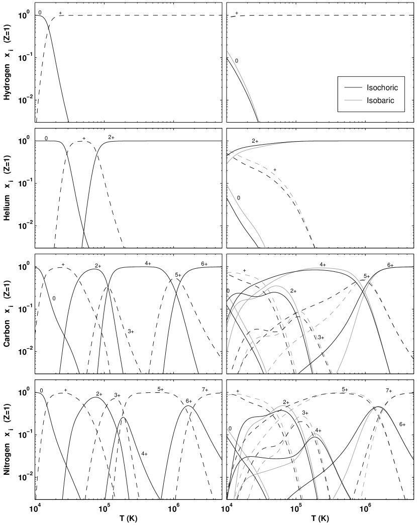
Figure 2.— Ion fractions $x_{i}\equiv n_{i,m}/n_{\rm H}A_{\rm m}$, versus gas temperature. Each row displays results for a different element. Left hand panels are for collisional ionization equilibrium (CIE). Right hand panels are for non-equilibrium isochoric and isobaric cooling for $Z=1$ times solar metallicity gas. Dark curves are for isochoric cooling. Light curves are for isobaric cooling. Panels show H, He, C, and N.

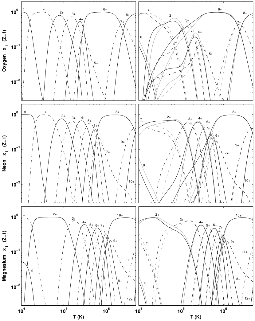
Figure 2.— Continued. Panels show O, Ne, and Mg.

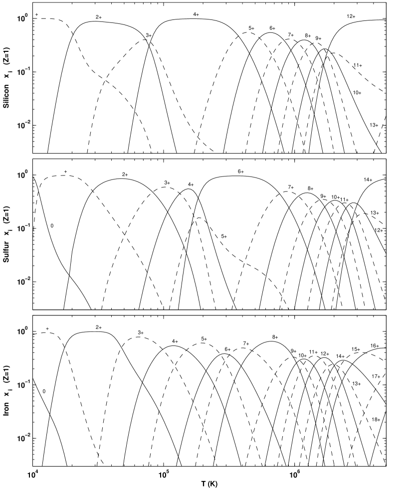
Figure 2.— Continued. Panels show CIE ion fractions for Si, S, and Fe.

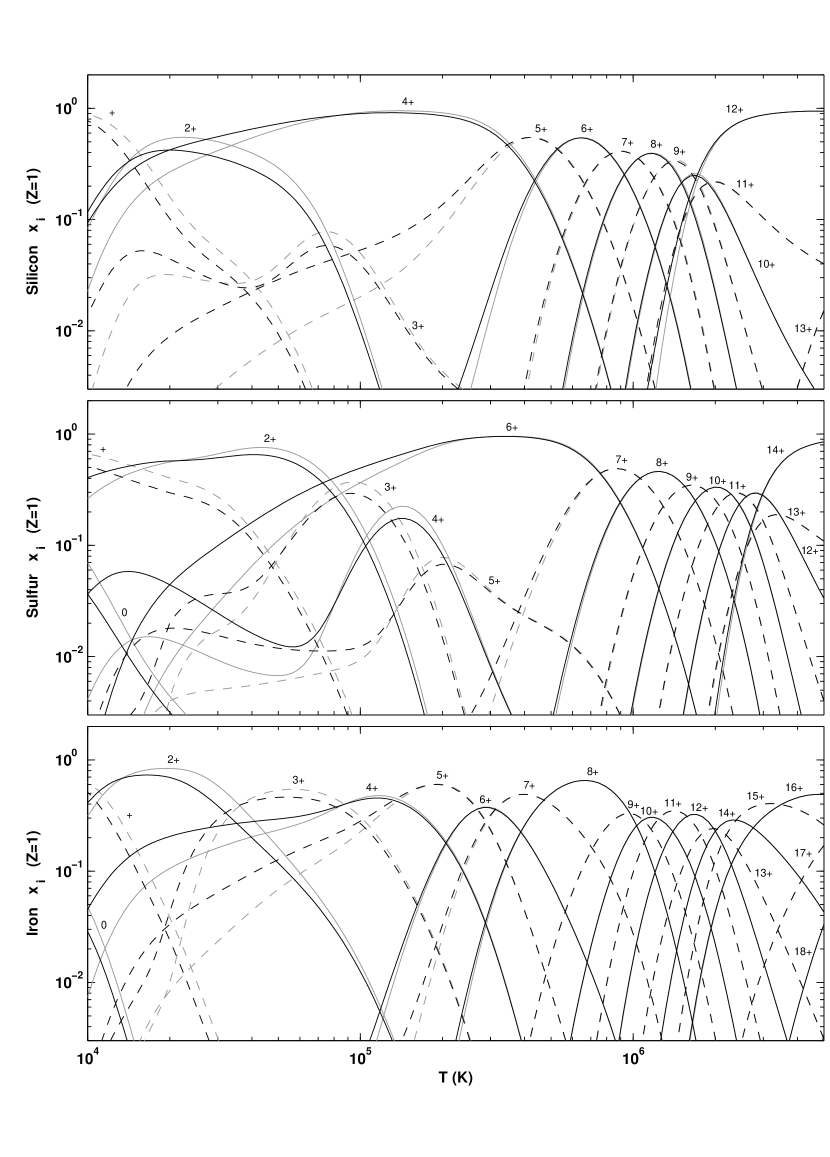
Figure 2.— Continued. Panels show time-dependent ion fractions for Si, S, and Fe.

curves therefore converge to specific “primordial” forms, which may or may not approach the CIE distributions. This depends on whether the low-$Z$ cooling time is long or short compared to the ion recombination time. For example, Figure 7a shows that at low $Z$, the O⁵⁺ fractions approach CIE. However, Figure 7b shows that O⁺⁺ remains out of equilibrium in the low-$Z$ limit. This is an example of an ion whose abundance distribution can never reach equilibrium, for any $Z$, in radiatively cooling gas. Such ions are generally those that appear at $T\lesssim 2\times 10^{5}$ K, where the low-$Z$ cooling times remain sufficiently short due to efficient cooling by hydrogen and helium Ly$\alpha$ emissions (see §5).

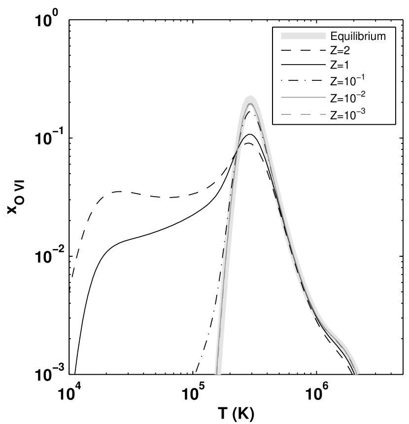
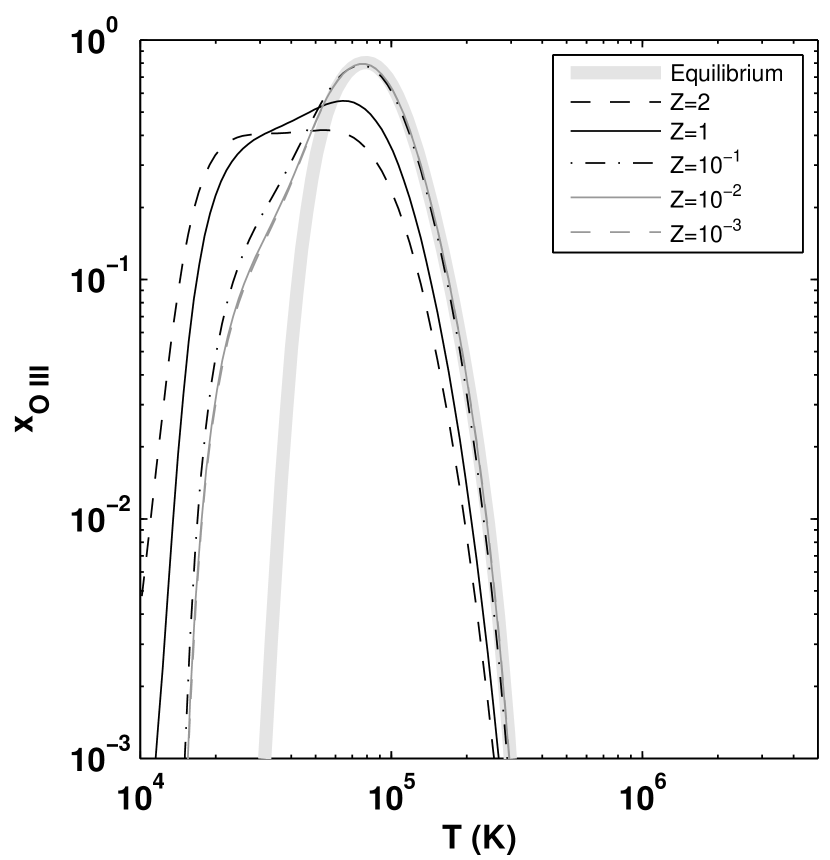
Figure 7.— O⁵⁺ (left) and O⁺⁺ (right) ion fractions versus temperature for metallicities $Z$ ranging from $10^{-3}$ to $2$, for isochoric cooling. The CIE distributions are shown by the thick grey lines.

5. Cooling Efficiencies

We have carried out computations of the cooling efficiencies $\Lambda(T,x_{i},Z)$ (erg cm³ s^-1) assuming CIE at all temperatures, and for time-dependent radiative cooling for isobaric and isochoric evolutions. Our results are displayed in Figure 8, and listed in Tables 13-15. The upper panel of Figure 8 shows our CIE cooling functions, $\Lambda_{\rm eq}$, for $T$ between $10^{4}$ and $10^{8}$ K, and $Z$ from $10^{-3}$ to $2$. The lower panel displays the non-equilibrium cooling curves.

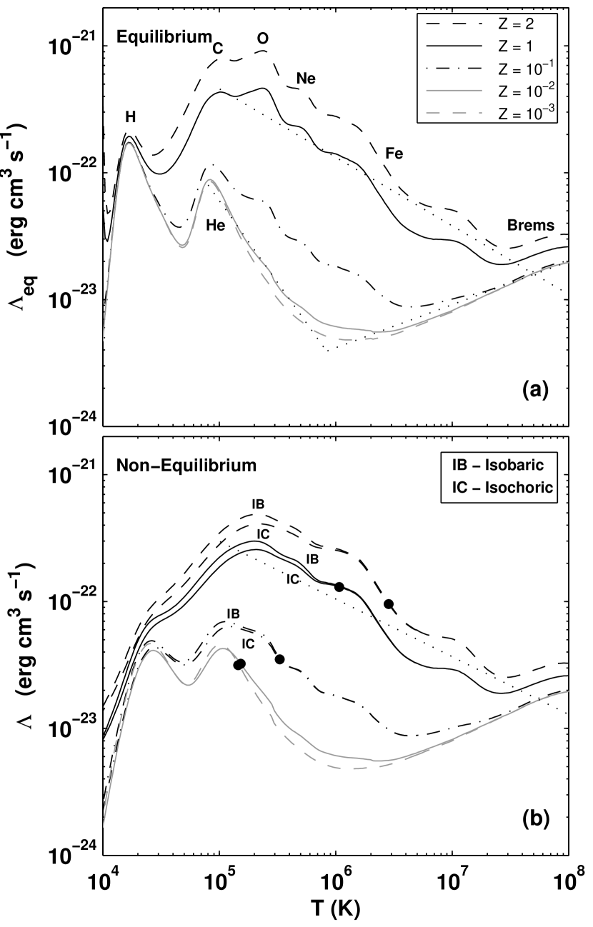
Figure 8.— Cooling efficiency (erg cm³ s^-1) versus temperature for $Z$ from $10^{-3}$ to $2$ times solar. (a) Equilibrium cooling. The dominant cooling elements at various temperatures are indicated near the curves. The dotted lines are our power-law fits for $Z=1$ and $Z=10^{-3}$, as given by equations 14 and 15. (b) Non-equilibrium cooling. For each $Z$, two curves are displayed: the lower curve is for isochoric (IC) cooling, and the upper curve is isobaric (IB) cooling. The dotted line is our power-law fit for $Z=1$ as given by equation 16. The filled circles indicate the temperatures where time-dependent cooling first deviate from the equilibrium cooling by 5%.

Table 13CIE Cooling Efficiencies

Temperature	$\Lambda(Z=10^{-3})$	$\Lambda(Z=10^{-2})$	…
(K)	(erg cm3 s-1)	(erg cm3 s-1)	…
$1.00\times 10^{4}$	$4.70\times 10^{-24}$	$4.98\times 10^{-24}$	…
$1.05\times 10^{4}$	$7.62\times 10^{-24}$	$7.79\times 10^{-24}$	…
$1.10\times 10^{4}$	$1.23\times 10^{-23}$	$1.25\times 10^{-23}$	…
$1.15\times 10^{4}$	$1.97\times 10^{-23}$	$1.98\times 10^{-23}$	…
$1.20\times 10^{4}$	$3.08\times 10^{-23}$	$3.09\times 10^{-23}$	…

Note. — The complete version of this table is in the electronic edition of the Journal. The printed edition contains only a sample.

In computing the CIE cooling efficiencies we use the equilibrium ion fractions $x_{i}^{\rm eq}(T)$ computed in §4 as inputs to the cooling functions. Our CIE results reproduce the standard “cosmic cooling curves” presented in many previous papers in the literature (see §1). Small differences compared to previous calculations are expected due to updates in the input atomic data and in the assumed gas phase abundances of the heavy elements.

For $Z\gtrsim 0.1$, the radiative energy losses between $10^{5}$ and $\sim 10^{7}$ K are dominated by electron impact excitations of resonance line transitions of metal ions. Above $\sim 10^{7}$ K, metal line cooling becomes less effective, and bremsstrahlung radiation dominates. The low-temperature peak at $2\times 10^{4}$ K is mainly due to hydrogen Ly$\alpha$ cooling, a process that becomes less effective at higher temperatures where the neutral hydrogen fraction becomes small. Recombinations and forbidden-line transitions are minor contributors to the gas cooling. The familiar peaks and features in the cooling curves are due to specific metal line coolants that dominate at different temperatures. The Ly$\alpha$ maximum is followed by peaks at $1.0\times 10^{5}$, $3.0\times 10^{5}$, $5.0\times 10^{5}$, and $1.5\times 10^{6}$, due respectively to resonance line transitions of carbon, oxygen, neon, and iron ions. For $Z=1$ we find a maximum equilibrium cooling efficiency of $4.6\times 10^{-22}$ erg cm³ s^-1 at $T=2.3\times 10^{5}$ K.

For $Z\lesssim 0.01$, metal cooling becomes negligible, and the energy losses are dominated by hydrogen and helium only. H, He and He⁺ line emissions dominate at low $T$, and electron bremsstrahlung due to scattering with H⁺ and He⁺⁺ at high $T$. The cooling peak at $10^{5}$ K that appears when $Z$ becomes small, is due to He⁺ Ly$\alpha$.

Between $10^{5}$ and $10^{8}$ K, our $Z=1$ cooling function is well fit by the power-law expression (cf. Kahn et al. 1976),

$$\Lambda_{\rm eq}^{Z=1}=2.3\times 10^{-19}~{}T^{-0.54}\ \ \ \ {\rm erg\ cm^{3}\ s^{-1}\ .}$$ (14)

This approximation is accurate to within a factor of $2.4$ over this temperature range ($10^{5}<T<10^{8}$ K), and to within a factor of 1.7 for $10^{5}<T<6.3\times 10^{7}$ K. For $Z\gtrsim 1$, and between 10⁵ and $\sim 10^{7}$ K, $\Lambda$ is linearly proportional to $Z$. For this range of parameters it follows from equations (14) and (8) that the cooling time $t_{c}\simeq 0.22~{}T_{6}^{1.54}/(n\,Z)$ Myr for isochoric cooling, and a factor 1.6 times longer for isobaric cooling.

For $Z\lesssim 0.01$, the cooling efficiency is independent of $Z$. In this low-Z limit, the two-piece power law

$$\Lambda_{\rm eq}^{Z=10^{-3}}=\left\{\begin{array}[]{lcl}1.7\times 10^{-16}~{}T^{-1.29}&,&8\times 10^{4}<T<8\times 10^{5}~{}{\rm K}\\ 3.8\times 10^{-26}~{}T^{~{}0.34}&,&8\times 10^{5}<T<10^{8}~{}{\rm K}\end{array}\right.$$ (15)

(in units of erg cm³ s^-1) reproduces the CIE cooling efficiency between $8\times 10^{4}$ and $10^{8}$ K to within a factor of 1.35.

Figure 8b displays our results for the non-equilibrium cooling efficiencies. In these computations we use the non-equilibrium ion fractions, $x_{i}(T)$, obtained by solving the coupled equations (1) and (5), as presented in §4, to compute $\Lambda(T,x_{i},Z)$. For each $Z$ we assume sufficiently large initial temperatures such that ionization equilibrium is established before significant cooling begins. Departures from equilibrium then occur as the temperature drops and the cooling times become short. For each $Z$ the filled circles in Figure 8b indicate the points where the cooling curves begin to deviate by more than 5% from CIE cooling. This is also where the isobaric and isochoric cooling curves (indicated for each $Z$ by the labels “IB” and “IC”) bifurcate. For $Z=1$, departures from equilibrium set in for $T\lesssim 10^{6}$ K. The deviations from CIE cooling begin at higher temperatures for higher $Z$, and lower temperatures for lower $Z$. For temperatures above the “departure points” the curves in the upper and lower panels of Figure 8 are identical.

There are several important differences between the non-equilibrium and CIE cooling curves. First, the distinct peaks and features that appear for CIE are smeared out in the non-equilibrium cooling curves. This is due to the broader ion distributions, $x_{i}(T)$, that occur for non-equilibrium cooling. Individual ions then contribute to the cooling over a larger temperature range. For example, for non-equilibrium cooling at high $Z$ ions such as O⁺⁺ and Ne⁺⁺ persist below $10^{5}$ K, where they contribute significantly to the cooling in addition to Ly$\alpha$. The Ly$\alpha$ cooling peak is itself broadened because a high electron fraction is maintained down to low temperatures.

Second, the non-equilibrium cooling efficiencies are suppressed, by factors of 2 to 4, compared to CIE cooling. For example, for $Z=1$ the maximum non-equilibrium cooling efficiency, occurring at $T=2.1\times 10^{5}$ K, is reduced to $2.6\times 10^{-22}$ erg cm³ s^-1, a factor of 1.8 less than the maximal CIE efficiency. The suppression occurs because the gas remains “over-ionized” as it cools, and the densities of the specific coolants that are most effective at each temperature are reduced. The more highly ionized species that remain present at each temperature generally have more energetic resonance line transitions, and these are less efficiently excited by the thermal electrons (McCray 1987). For example, for non-equilibrium cooling in the low-$Z$ limit the absolute and relative heights of the hydrogen and helium Ly$\alpha$ peaks are reduced compared to CIE cooling. This is because the H⁰ and He⁺ fractions remain smaller at any temperature compared to CIE.

Third, because isochoric cooling is faster (see equation [8]) with correspondingly greater recombination lags, the suppressions in the cooling efficiencies are larger, and the isochoric curves fall below the isobaric curves.

The differences we find between CIE and non-equilibrium cooling, are in good agreement with the results found by Sutherland & Dopita (1993; see their Fig. 13) and Schmutzler & Tscharnuter (1993; see their Fig. 2.2). For $Z=1$ the power-law expression

$$\Lambda_{\rm non-eq}^{Z=1}~{}=~{}5.6\times 10^{-20}~{}T^{-0.46}\ \ \ {\rm erg\ cm^{3}\ s^{-1}}$$ (16)

provides a good fit to the non-equilibrium cooling efficiency between $10^{5}$ and $10^{8}$ K, and is accurate to within a factor of 2.2. For $10^{5}<T<5.5\times 10^{7}$ K, it is accurate to within a factor of 1.5. For low-$Z$, departures from CIE cooling occur only below $2\times 10^{5}$ K, so that the fit given by equation (15) remains valid for radiatively cooling gas at low metallicity, for $T>2\times 10^{5}$ K.

The suppression of the cooling efficiencies compared to CIE implies longer cooling times. The actual recombination lag is therefore smaller than would occur if the gas were able to cool at the faster CIE rates. The departures from ionization equilibrium are thus stabilized by the reduction in the cooling rates.

6. Diagnostics

For a uniformly cooling gas cloud, the line-of-sight column densities of ions $i$ of element $m$ may be expressed simply as $N_{i}^{m}=A_{m}x_{i}(T)N_{\rm H}$, where $N_{\rm H}$ is the column density of hydrogen nuclei, $A_{m}$ is the abundance of element $m$ (relative to H), and $x_{i}(T)$ are the temperature-dependent ion fractions, as computed in §4. Specific column density ratios

$$\frac{N^{m}_{i}}{N^{n}_{j}}=\frac{A_{m}}{A_{n}}\frac{x_{i}(T)}{x_{j}(T)}$$ (17)

may therefore be used as diagnostic probes of the ionization state, temperature, and also metallicity in radiatively cooling gas. For CIE, the ion fractions are independent of the metallicity $Z$, and the column density ratios depend only on the gas temperature (and the relative elemental abundances $A_{m}/A_{n}$). However, for non-equilibrium cooling the ion fractions also depend on $Z$, and hence so do the column density ratios.

Diagnostic diagrams for radiatively cooling gas for different metallicities, may be constructed using the computational data we presented in §4 (Figs. 2-6 and Tables 2-12). As an example , in Figure 9 we display “cooling trajectories” for $N_{\rm C~{}IV}/N_{\rm O~{}VI}$ versus $N_{\rm N~{}V}/N_{\rm O~{}VI}$, for $T$ ranging from $5\times 10^{6}$ to $10^{4}$ K. The gas temperature is represented by color along the curves, from hot (red) to cool (blue). Panel (a) shows the behavior for CIE, for which the results are independent of $Z$. Panels (b)-(f) are for non-equilibrium isochoric cooling, for $Z$ from $10^{-3}$ to $2$. The CIE trajectory is reproduced as the grey curves in panels (b)-(f).

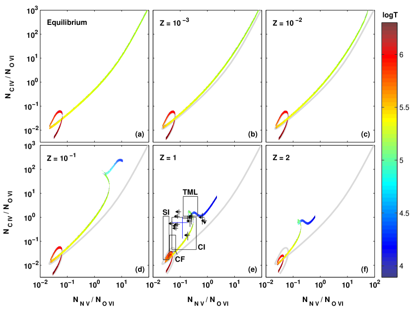
Figure 9.— Column density ratios $N_{\rm C~{}IV}/N_{\rm O~{}VI}$ versus $N_{\rm N~{}V}/N_{\rm O~{}VI}$ for radiatively cooling gas. Gas temperature is indicated by color along the trajectories, from hot (red) to cool (blue). Temperature versus color legend is on the right. (a) displays the CIE trajectory, shown again as grey curves in the other panels. (b)-(f) are the trajectories non-equilibrium isochoric cooling for different values of the metallicity $Z$. The data points (Fox et al. 2005) show the ionic ratios observed in metal absorbers toward HE 0226-4110 and PG 0953+414 (black), and in the Galactic halo (blue). The boxes show model prediction, as demarcated by Fox et al., for turbulent mixing layers (TMLs), conductive interfaces (CIs), cooling flows (CFs) and shock ionization (SI).

For the $Z$=1 model in Figure 9 we also display, as observational examples, the data points and upper limits presented by Fox et al. (2005) for the multiphased high-velocity cloud absorbers towards the background sources HE 0226-4110 and PG 0953+414 (black crosses). The plot also includes the Galactic halo average (blue cross) $N_{\rm C~{}IV}/N_{\rm O~{}VI}=0.6\pm 0.47$ and $N_{\rm N~{}V}/N_{\rm O~{}VI}=0.12\pm 0.07$ (Zsargó et al. 2003, as quoted by Fox et al.). We also show the regions demarcated by Fox et al. for the predictions for a variety of ionization mechanisms, including turbulent mixing layers (TMLs; Slavin, Shull, & Begelman 1993), conductive interfaces (CIs; Borkowski, Balbus, & Fristrom 1990), cooling flows (CFs; Edgar & Chevalier 1986) and shock ionization (SI; Dopita & Sutherland 1996).

To set the absolute scale of our predicted ion columns, in Figure 10 we plot $N_{\rm C~{}IV}/N_{\rm O~{}VI}$ versus $N_{\rm O~{}VI}/N_{{\rm H},20}$ for each $Z$, where $N_{{\rm H},20}$ is the hydrogen column density in units of $10^{20}$ cm^-2. For the CIE calculation we assume $Z=1$. At any temperature, the O VI column scales linearly with the assumed $N_{\rm H}$, whereas the column density ratios are independent of $N_{\rm H}$.

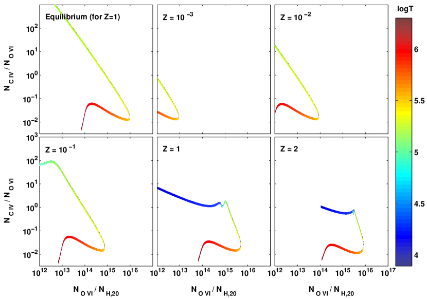
Figure 10.— Same as Figure 9 but for column density ratio $N_{\rm C~{}IV}/N_{\rm O~{}VI}$ versus $N_{\rm O~{}VI}/N_{{\rm H},20}$, where $N_{{\rm H},20}$ is the hydrogen column density in units of $10^{20}$ cm^-2.

Of the three ions we are considering, O⁵⁺ is the most highly ionized, so that C IV/O VI and N V/O VI are small at high temperature, and become large at low temperature. Figures 9 and 10 show again that for time-dependent radiative cooling the gas remains more highly ionized compared to CIE. As $Z$ becomes large and the recombination lags grow, the ion ratios remain small even at low temperatures. The cooling trajectories are therefore confined to a narrower range of ion ratios for non-equilibrium cooling. Furthermore, in our example, it is evident that for a given N V/O VI ratio, the associated C IV/O VI ratio is larger for non-equilibrium cooling compared to CIE. For example, a cloud for which $N_{\rm N~{}V}/N_{\rm O~{}VI}\simeq 3$ and $N_{\rm C~{}IV}/N_{\rm O~{}VI}\simeq 30$ would be inconsistent with gas at CIE at any temperature, yet consistent with isochoric radiatively cooling gas at a temperature near $\sim 1.3\times 10^{5}$ K. It is clear that assuming CIE when interpreting such data may lead to significant inaccuracies. For example, for an isochorically cooling cloud with $Z\simeq 1$, absorption line measurements yielding $N_{\rm C~{}IV}/N_{\rm O~{}VI}\approx 1$ and $N_{\rm N~{}V}/N_{\rm O~{}VI}\approx 1$ would be interpreted as indicating $T\simeq 2\times 10^{5}$ K assuming CIE, whereas in fact these ratios occur at a much lower temperature $\sim 10^{4}$ K.

Interestingly, many (but not all) of the Fox et al. (2005) data points lie close to our $Z=1$ cooling trajectory (see Figure 9e). At lower metallicities the column density ratios approach the CIE trajectory which lies well below the data points. However, as indicated by Figure 9e, even for $Z=1$ further constraints may be required to distinguish radiatively cooling gas from ionization occurring in conductive interfaces or turbulent mixing layers.

7. Summary

In this paper we present new computations of the equilibrium and non-equilibrium cooling efficiencies and ionization states for low-density radiatively cooling gas, containing cosmic abundances of the elements H, He, C, N, O, Ne, Mg, Si, S, and Fe. In these calculations we assume pure radiative cooling, with no gas heating or photoionization by external sources. We present results for gas temperatures, $T$, between 10⁴ and 10⁸ K. We assume that the gas is dust free, and we consider metallicities $Z$ ranging from 10^-3 to 2 times the elemental abundances in the Sun. We carry out our computations using up-to-date rate coefficients for all of the atomic recombination and ionization processes, and the energy loss mechanisms.

For temperatures below $\sim 5\times 10^{6}$ K, where ion-electron recombination lags significantly behind the cooling, we explicitly solve the coupled time-dependent ionization and energy loss equations for the cooling gas. For such gas we assume that the cooling is from an initially hot equilibrium state. The basic equations and our numerical method are presented in §2. We calculate the non-equilibrium cooling efficiencies for constant pressure (isobaric) and constant density (isochoric) evolutions. Departures from collisional ionization equilibrium (CIE) are slightly smaller for isobaric cooling.

In §3 we consider the conditions for isochoric versus isobaric cooling. We compute the critical column densities and temperatures at which the cooling time becomes short compared to the dynamical time, and the transition from isobaric to isochoric evolution occurs. These results are displayed in Figure 1, and are based on the cooling efficiencies we present in §5.

Because we exclude photoionization by external radiation, both the equilibrium and time-dependent behavior is independent of the assumed density or pressure. The primary parameter for radiative cooling is the metallicity. Departures from equilibrium are largest for high $Z$ where the ratios of the cooling and recombinations times are smallest. At very low metallicity ($Z\lesssim 10^{-2}$) the cooling rates, and hence also the recombination lags, are independent of the metallicity. In this limit any departures from CIE approach a universal “primordial” form. The results of our equilibrium ionization calculations are displayed in Figure 2 in §4. This figure also shows the ionization states for non-equilibrium isobaric and isochoric cooling, for $Z=1$. Results for other metallicities are presented in on-line tables and figures, as summarized in Table 16. Our computational data set can also be found at our website http://wise-obs.tau.ac.il/$\sim$orlyg/cooling/.

Table 16Ionization and Cooling Data

Data		Table	Figure
Ion Fractions:
CIE		$2$	$2$
$Z=1$,	Isochoric	$3$	$2$
$Z=1$,	Isobaric	$4$	$2$
$Z=10^{-3}$,	Isochoric	$5$	$3$
$Z=10^{-3}$,	Isobaric	$6$	$3$
$Z=10^{-2}$,	Isochoric	$7$	$4$
$Z=10^{-2}$,	Isobaric	$8$	$4$
$Z=10^{-1}$,	Isochoric	$9$	$5$
$Z=10^{-1}$,	Isobaric	$10$	$5$
$Z=2$,	Isochoric	$11$	$6$
$Z=2$,	Isobaric	$12$	$6$
Cooling Efficiencies:
CIE		$13$	$8$
Isochoric		$14$	$8$
Isobaric		$15$	$8$

Figure 8 in §5 displays our results for the equilibrium and non-equilibrium cooling efficiencies for $Z$ between 10^-3 and $2$. We provide simple, or two-piece, power-law fits (equations [14], [15], and [16]) for the equilibrium and non-equilibrium cooling efficiencies at high and low $Z$. Non-equilibrium cooling is suppressed, by factors of 2 to 4, relative to CIE, because of the generally higher ionization state of the rapidly cooling gas. The familiar peaks in the CIE cooling curve are smeared out for non-equilibrium cooling, because individual ions persist for a broader range of temperatures. Overall, our results are in good agreement with previous such calculations. Detailed difference are mainly due to differences in the input atomic data, and assumed abundances of the heavy elements. We make some explicit comparisons with previous computations in §4 and §5.

Ion ratios are useful as diagnostic probes. In §6 we discuss one example, N V/O VI versus C IV/OVI, and show how this ratio evolves in radiatively cooling gas, and how it can be used as a probe of metallicity for realistic non-equilibrium conditions.

In our computations we assume that the cooling gas is optically thin. In the Appendix, we provide numerical estimates for the maximal cloud column densities for which this assumption remains valid. We also investigate how reabsorption of hydrogen and helium recombination radiation in optically thick clouds alters the cooling rates and associated ionization states in non-equilibrium cooling gas. For high metallicity the effects of trapping are small, but become more significant ($\sim$ factors of 2) for low $Z$ gas.

In a companion paper we will present computations of the metal ion “cooling columns” produced in steady flows of radiative cooling gas, such as occur in post shock cooling layers, including the effects of “upstream” cooling radiation on the “downstream” ionization states. We will also consider how photoionization by external background radiation fields alters the ionization and thermal evolution of radiatively cooling gas such as we have considered here.

Appendix A Reabsorption of Diffuse Radiation Fields

In the computations presented in §4 and §5 we have assumed that the cooling gas is optically thin, and that reabsorption of line and continuum radiation emitted by the cooling gas may be ignored. In this Appendix we provide numerical estimates for the maximal cloud column densities for which the optically thin assumption is justified. We then examine how trapping of hydrogen and helium recombination radiation in optically thick clouds affects the time-dependent cooling efficiencies and ionization states.

For sufficiently large cloud column densities, absorption of the internally generated “diffuse radiation” can alter the ionization state in such a way as to enhance or reduce the net cooling rate. To estimate the critical column densities at which the cooling rates are altered, we use Cloudy to compute the local CIE cooling rates as functions of the total hydrogen column density, $N_{\rm H}$, for one-dimensional constant temperature slabs. We set the external radiation field to zero, so that the radiative transfer handled by Cloudy is for the internally generated diffuse fields only. For each temperature, $T$, and assumed metallicity $Z$, we identify the critical column density, $N_{\rm Hcrit}(T,Z)$, at which the local cooling efficiency at the cloud center first deviates by $50\%$ from the optically thin cooling rate at the cloud edge.

The critical column densities defined in this way are sensitive to the gas temperature and associated ionization states. Here we are not interested in the detailed fluctuations of $N_{\rm Hcrit}$ with gas temperature, but rather with the broad trends. In Figure 11, we display a smoothed representation of $N_{\rm Hcrit}$ versus $T$. The solid curve, appearing for $T\lesssim 6\times 10^{4}$ K is for the entire metallicity range $10^{-3}<Z<2$. For higher temperatures, the behavior is sensitive to $Z$, and we display the critical columns by dashed lines for selected metallicity ranges. For temperatures where no curves appear in Figure 11 the critical columns exceed $10^{24}$ cm^-2.

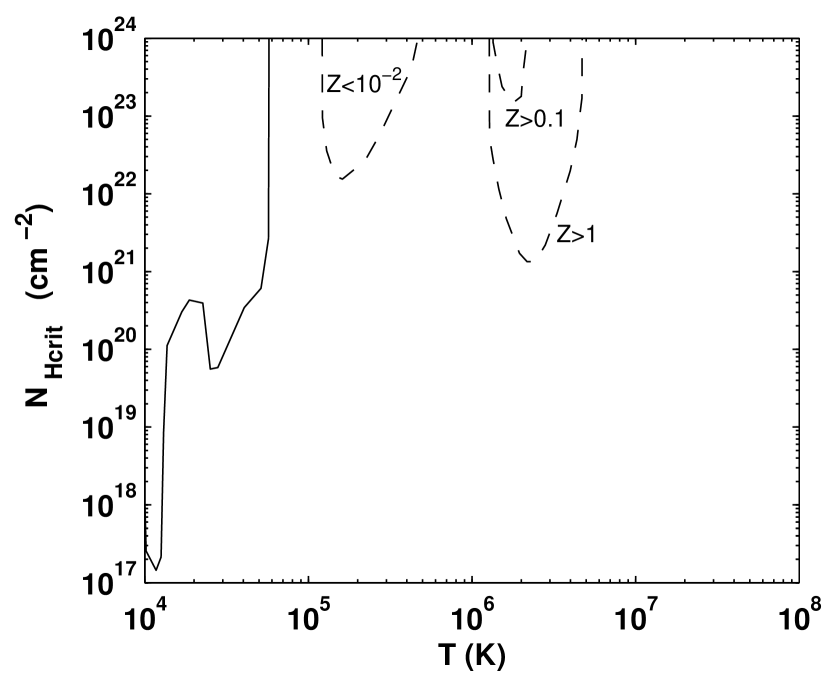
Figure 11.— $N_{\rm Hcrit}$ versus temperature. $N_{\rm Hcrit}$ is the column density at which the cooling deviates by $50\%$ from the optically thin value (see text). The solid curve is for all metallicities $10^{-3}<Z<2$. The dashed curves are for the displayed $Z$ range. For temperatures where no curve is displayed, $N_{\rm Hcrit}>10^{24}$ cm^-2.

Three distinct regimes appear in Figure 11. For $10^{4}\lesssim T\lesssim 6\times 10^{4}$ K, a transition from “case A” to “case B” hydrogen recombination occurs as the cloud becomes optically thick. Photoionization of hydrogen by H⁺ and He⁺ recombination radiation then alters the dominating Ly$\alpha$ cooling rate. The Ly$\alpha$ cooling rate is proportional to the product $x_{\rm e}(1-x_{\rm e})$, where $x_{\rm e}$ is the electron fraction. For $T\lesssim 1.5\times 10^{4}$ K, the neutral fraction $(1-x_{\rm e})\approx 1$, whereas $x_{\rm e}$ increases in the transition to case B. This leads to increased Ly$\alpha$ cooling. At these low temperatures we find that $N_{\rm Hcrit}\sim 10^{17}$ cm^-2. At higher temperatures, $T\gtrsim 2.5\times 10^{4}$ K, the hydrogen is largely ionized and $x_{\rm e}\approx 1$ so the transition to case B mainly reduces the neutral fraction $(1-x_{\rm e})$. This leads to decreased Ly$\alpha$ cooling. For $T=2.5\times 10^{4}$ K, we find $N_{\rm Hcrit}\approx 5\times 10^{19}$ cm^-2. Between these two temperatures, $x_{\rm e}(1-x_{\rm e})$ remains approximately constant in the transition to case B, and a local maximum of $N_{\rm Hcrit}=4\times 10^{20}$ cm^-2 appears at $T\approx 2\times 10^{4}$ K. Above $T\sim 6\times 10^{4}$ K $N_{\rm Hcrit}$ rises sharply because the hydrogen becomes so highly ionized that Ly$\alpha$ cooling is no longer the dominant coolant.

Similarly, absorption of He⁺⁺ recombination radiation by He⁺ ions alters the He⁺ Ly$\alpha$ cooling rate at temperatures near 10⁵ K where helium makes the transition from singly to doubly ionized form. However, this effect is only important for low metallicity ($Z<10^{-2}$) clouds, where He⁺ Ly$\alpha$ is a significant coolant. For such clouds, $N_{\rm Hcrit}=1.5\times 10^{22}$ cm^-2 at $T=1.6\times 10^{5}$ K.

Finally, for $10^{6}\lesssim T\lesssim 5\times 10^{6}$ K, we find that $N_{\rm Hcrit}\sim 10^{21}$ cm^-2 in high metallicity ($Z~{}\gtrsim~{}1$) clouds. At these temperatures, photoionization by numerous energetic metal emission lines ionize O⁷⁺, and shift the peak of the iron ion distribution from Fe¹¹⁺-Fe¹⁴⁺ to Fe¹³⁺-Fe¹⁶⁺. This reduces the cooling rate, because O⁷⁺, Fe¹¹⁺, and Fe¹²⁺ are dominant coolants at these temperatures. For lower $Z$, bremsstrahlung cooling plays a more dominant role, and photoionization of the oxygen and iron ions is less important, so $N_{\rm Hcrit}$ is much larger.

Our computations for $N_{\rm Hcrit}$ in Figure 11 are for CIE conditions. We now examine how trapping of hydrogen and helium recombination radiation alters the cooling efficiencies and non-equilibrium ionization states for time-dependent cooling. We consider a series of isochoric model clouds with total column densities ranging up to $N_{\rm H}=10^{24}$ cm^-2. We assume that the H⁺, He⁺, and He⁺⁺ recombination photons are reabsorbed on-the-spot when the photoionization optical depths at the H⁰, He⁰ and He⁺ ionization thresholds exceed unity respectively. The critical temperatures below which the clouds become optically thick are higher for clouds with larger total column densities, since lower neutral hydrogen and helium fractions are required. When the clouds become optically thick we switch from case A to case B recombination in computing the evolution of the hydrogen and helium ionization states.

In Figure 12 we plot the neutral hydrogen fractions, $x_{\rm H}(T)$, and cooling efficiencies, $\Lambda(T)$, for case A and case B recombination. We display results for $Z=1$ (left-hand panels), and for $Z=10^{-3}$ (right-hand panels). To illustrate the effects on the metal ion distributions we also plot the C⁺, C⁺⁺, and C³⁺ fractions.

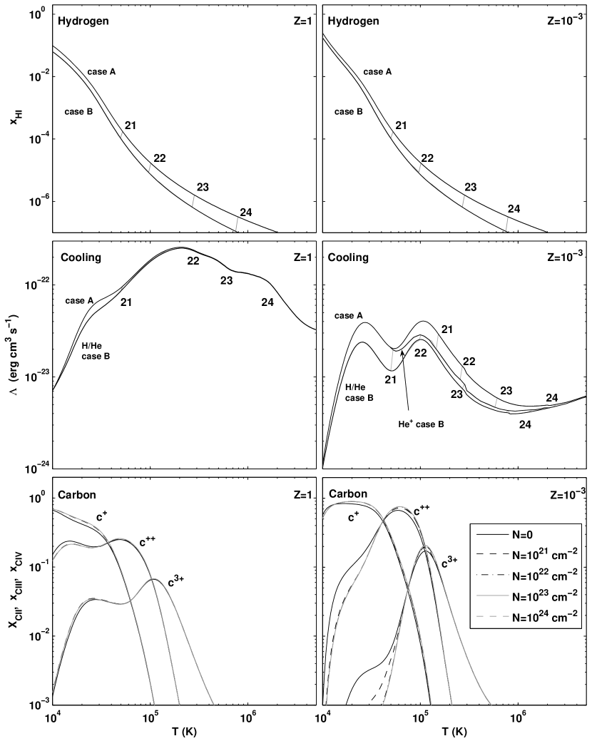
Figure 12.— Ionization and cooling in optically thin and thick clouds. Left hand panels are for $Z=1$. Right hand panels are for $Z=10^{-3}$. Upper row shows the neutral hydrogen fractions versus temperature for optically thin “case A”, and optically thick “case B” (see text). The vertical lines mark the temperatures at which the gas becomes optically thick for different total cloud column densities, as indicated by the adjacent labels showing $log(N_{\rm H})$. Middle row displays the optically thin and thick cooling efficiencies. For $Z=10^{-3}$ the intermediate curve is for a cloud that is optically thick only to He⁺⁺ recombination radiation (see text). Lower row displays the C⁺, C⁺⁺, and C³⁺ ion fractions for optically thin and thick clouds.

The neutral hydrogen fractions are, of course, reduced in optically thick clouds. The vertical lines connecting the case A and case B curves indicate the temperatures at which, for a given total cloud column $N_{\rm H}$, the cloud becomes optically thick to hydrogen recombination radiation. For example, for $N_{\rm H}=10^{21}$ cm^-2, this occurs at $T=5\times 10^{4}$ K.

For $Z=1$ the differences between case A and case B cooling are small, and are only apparent at low temperatures where Ly$\alpha$ cooling dominates. For non-equilibrium cooling the electron fraction remains large down to $10^{4}$ K. Therefore, down to this temperature Ly$\alpha$ cooling is reduced by the reduction in the neutral H fraction. (This is opposed to the situation in CIE where, as discussed above, for $10^{4}$ K gas the Ly$\alpha$ cooling is enhanced by an increased electron density in optically thick clouds.) For $Z=1$, the slightly altered cooling efficiencies in optically thick clouds lead to only very small changes in the non-equilibrium metal ion abundances, as is illustrated for the carbon ions in Figure 12. Our conclusions for $Z=1$ are consistent with the results of Kafatos (1973) and Shapiro & Moore (1976), who considered the transition from optically thin to thick (for hydrogen recombination radiation only) at a single temperature $T=3.5\times 10^{4}$ K (corresponding to $N_{\rm H}\approx 1.3\times 10^{20}$ cm^-2).

For $Z=10^{-3}$, hydrogen and helium are already the dominant emission line coolants below $\sim 10^{6}$ K, and the transition to optically thick conditions has a larger effect. The cooling efficiencies are reduced by up to a factor $\sim 2$. In Figure 12 we draw three cooling curves for $Z=10^{-3}$. The upper curve is for optically thin case A cooling. The middle curve (labeled “He⁺ case B”) is for clouds that are still optically thin to H⁺ and He⁺ recombination radiation, but are thick to He⁺⁺ recombination photons. The lower curve is for case B clouds that are thick to the H⁺ and He⁺ recombination photons as well. The vertical lines connecting the curves indicate the transition temperatures for different cloud columns $N_{\rm H}$. For example, a $10^{21}$ cm^-2 cloud shifts from case A to “He⁺ case B” at $\sim 2\times 10^{5}$ K, and then becomes thick to H⁺ and He⁺ recombination radiation (“H/He case B”) at $\sim 5\times 10^{4}$ K.

For low-$Z$ gas the overall cooling rates are small, and hence so are the departures from CIE. Therefore, even though the cooling efficiencies are significantly altered by trapping of the recombination radiation, the resulting effect on the ion fractions is not very large. As shown for C⁺, C⁺⁺, and C³⁺ the effects are most significant at low temperatures where the departures from CIE are largest.

References

- Aldrovandi & Pequignot (1973) Aldrovandi, S. M. V., & Pequignot, D. 1973, A&A, 25, 137
- Allen & Dupree (1969) Allen, J. W., & Dupree, A. K. 1969, ApJ, 155, 27
- Altun et al. (2004) Altun, Z., Yumak, A., Badnell, N. R., Colgan, J., & Pindzola, M. S. 2004, A&A, 420, 775
- Altun et al. (2005) Altun, Z., Yumak, A., Badnell, N. R., Colgan, J., & Pindzola, M. S. 2005, A&A, 433, 395
- Altun et al. (2006) Altun, Z., Yumak, A., Badnell, N. R., Loch, S. D., & Pindzola, M. S. 2006, A&A, 447, 1165
- Anders & Grevesse (1989) Anders, E., & Grevesse, N. 1989, Geochim. Cosmochim. Acta, 53, 197
- Antia & Basu (2005) Antia, H. M., & Basu, S. 2005, ApJ, 620, L129
- Arnaud & Raymond (1992) Arnaud, M., & Raymond, J. 1992, ApJ, 398, 394
- Arnaud & Rothenflug (1985) Arnaud, M., & Rothenflug, R. 1985, A&AS, 60, 425
- Asplund et al. (2005) Asplund, M., Grevesse, N., & Sauval, A. J. 2005a, ASP Conf. Ser. 336: Cosmic Abundances as Records of Stellar Evolution and Nucleosynthesis, 336, 25
- Asplund et al. (2005) Asplund, M., Grevesse, N., Gudel, M., & Sauval, A.J. 2005b, astro-ph/0510377
- Ayres et al. (2006) Ayres, T. R., Plymate, C., & Keller, C. U. 2006, ApJS, 165, 618
- Badnell et al. (2003) Badnell, N. R., et al. 2003, A&A, 406, 1151
- Badnell (2006) Badnell, N. R. 2006, A&A, 447, 389
- Ballantyne et al. (2000) Ballantyne, D. R., Ferland, G. J., & Martin, P. G. 2000, ApJ, 536, 773
- Bahcall et al. (2005) Bahcall, J. N., Basu, S., & Serenelli, A. M. 2005, ApJ, 631, 1281
- Benjamin et al. (2001) Benjamin, R. A., Benson, B. A., & Cox, D. P. 2001, ApJ, 554, L225
- Boehringer & Hensler (1989) Boehringer, H., & Hensler, G. 1989, A&A, 215, 147
- Borkowski et al. (1990) Borkowski, K. J., Balbus, S. A., & Fristrom, C. C. 1990, ApJ, 355, 501
- Bottcher et al. (1970) Bottcher, C., McCray, R.A., Jura, M., & Dalgarno, A. 1970, Ap.Lett., 6, 237
- Breitschwerdt & Schmutzler (1994) Breitschwerdt, D., & Schmutzler, T. 1994, Nature, 371, 774
- Breitschwerdt & Schmutzler (1999) Breitschwerdt, D., & Schmutzler, T. 1999, å, 347, 650
- Cen & Ostriker (1999) Cen, R., & Ostriker, J. P. 1999, ApJ, 514, 1
- Clarke et al. (1998) Clarke, N.J., et al. 1998, J. Phys. B: At. Mol. Opt. Phys. 33, 533
- Colgan et al. (2003) Colgan, J., Pindzola, M. S., Whiteford, A. D., & Badnell, N. R. 2003, A&A, 412, 597
- Colgan et al. (2004) Colgan, J., Pindzola, M. S., & Badnell, N. R. 2004, A&A, 417, 1183
- Colgan et al. (2005) Colgan, J., Pindzola, M. S., & Badnell, N. R. 2005, A&A, 429, 369
- Collins et al. (2005) Collins, J. A., Shull, J. M., & Giroux, M. L. 2005, ApJ, 623, 196
- Cox & Tucker (1969) Cox, D. P., & Tucker, W. H. 1969, ApJ, 157, 1157
- Dalgarno & McCray (1972) Dalgarno, A., & McCray, R. A. 1972, ARA&A, 10, 375
- Davé et al. (2001) Davé, R., et al. 2001, ApJ, 552, 473
- Draine (1981) Draine, B. T. 1981, ApJ, 245, 880
- Draine & McKee (1993) Draine, B.T., & McKee, C.F. 1993, ARA&A, 31, 373
- Dopita & Sutherland (1996) Dopita, M. A., & Sutherland, R. S. 1996, ApJS, 102, 161
- Drake & Testa (2005) Drake, J. J., & Testa, P. 2005, Nature, 436, 525
- Edgar & Chevalier (1986) Edgar, R. J., & Chevalier, R. A. 1986, ApJ, 310, L27
- Fang et al. (2006) Fang, T., Mckee, C. F., Canizares, C. R., & Wolfire, M. 2006, ApJ, 644, 174
- Ferland et al. (1997) Ferland, G. J., Korista, K. T., Verner, D. A., & Dalgarno, A. 1997, ApJ, 481, L115
- Ferland et al. (1998) Ferland, G. J., Korista, K. T., Verner, D. A., Ferguson, J. W., Kingdon, J. B., & Verner, E. M. 1998, PASP, 110, 761
- Fox et al. (2004) Fox, A. J., Savage, B. D., Wakker, B. P., Richter, P., Sembach, K. R., & Tripp, T. M. 2004, ApJ, 602, 738
- Fox et al. (2005) Fox, A. J., Wakker, B. P., Savage, B. D., Tripp, T. M., Sembach, K. R., & Bland-Hawthorn, J. 2005, ApJ, 630, 332
- Fox et al. (2006) Fox, A. J., Savage, B. D., & Wakker, B. P. 2006, ApJS, 165, 229
- Furlanetto et al. (2005) Furlanetto, S. R., Phillips, L. A., & Kamionkowski, M. 2005, MNRAS, 359, 295
- Gaetz & Salpeter (1983) Gaetz, T. J., & Salpeter, E. E. 1983, ApJS, 52, 155
- Gnat & Sternberg (2004) Gnat, O., & Sternberg, A. 2004, ApJ, 608, 229
- Heckman et al. (2002) Heckman, T. M., Norman, C. A., Strickland, D. K., & Sembach, K. R. 2002, ApJ, 577, 691
- Hindmarsh (1983) Hindmarsh, A. C., 1983, ODEPACK, A Systematized Collection of ODE Solvers, in Scientific Computing, R. S. Stepleman et al. (eds.), North-Holland, Amsterdam, 1983 (vol. 1 of IMACS Transactions on Scientific Computation), pp. 55-64.
- House (1964) House, L. L. 1964, ApJS, 8, 307
- Jordan (1969) Jordan, C. 1969, MNRAS, 142, 501
- Jura & Dalgarno (1972) Jura, M., & Dalgarno, A. 1972, ApJ, 174, 365
- Kafatos (1973) Kafatos, M. 1973, ApJ, 182, 433
- Kahn (1976) Kahn, F. D. 1976, A&A, 50, 145
- Kingdon & Ferland (1996) Kingdon, J. B., & Ferland, G. J. 1996, ApJS, 106, 205
- Landi & Landini (1999) Landi, E., & Landini, M. 1999, A&A, 347, 401
- Landini & Fossi (1991) Landini, M., & Fossi, B. C. M. 1991, A&AS, 91, 183
- Landini & Monsignori Fossi (1990) Landini, M., & Monsignori Fossi, B. C. 1990, A&AS, 82, 229
- Maller & Bullock (2004) Maller, A. H., & Bullock, J. S. 2004, MNRAS, 355, 694
- McCray (1987) McCray, R. 1987, in Spectroscopy of Astrophysical Plasmas, Eds. A. Dalgarno & D. Layzer (Cambridge University Press), p. 255
- Mitnik & Badnell (2004) Mitnik, D. M., & Badnell, N. R. 2004, A&A, 425, 1153
- Netzer et al. (2005) Netzer, H., Lemze, D., Kaspi, S., George, I. M., Turner, T. J., Lutz, D., Boller, T., & Chelouche, D. 2005, ApJ, 629, 739
- Nicastro et al. (2005) Nicastro, F., et al. 2005, Nature, 433, 495
- Ostriker & Silk (1973) Ostriker, J., & Silk, J. 1973, ApJ, 184, L113
- Osterbrock (1989) Osterbrock, D. E. 1989, Astrophysics of Gaseous Nebulae & Active Galactic Nuclei, (Mill Valley: University Science Books)
- Pequignot et al. (1991) Pequignot, D., Petitjean, P., & Boisson, C. 1991, A&A, 251, 680
- Rasmussen et al. (2006) Rasmussen, A. P., Kahn, S. M., Paerels, F., Willem den Herder, J., Kaastra, J., & de Vries, C. 2006, astro-ph/0604515
- Raymond et al. (1976) Raymond, J. C., Cox, D. P., & Smith, B. W. 1976, ApJ, 204, 290
- Richter et al. (2004) Richter, P., Savage, B. D., Tripp, T. M., & Sembach, K. R. 2004, ApJS, 153, 165
- Savage et al. (2002) Savage, B. D., Sembach, K. R., Tripp, T. M., & Richter, P. 2002, ApJ, 564, 631
- Savage et al. (2005) Savage, B. D., Lehner, N., Wakker, B. P., Sembach, K. R., & Tripp, T. M. 2005, ApJ, 626, 776
- Schmelz et al. (2005) Schmelz, J. T., Nasraoui, K., Roames, J. K., Lippner, L. A., & Garst, J. W. 2005, ApJ, 634, L197
- Schmutzler & Tscharnuter (1993) Schmutzler, T., & Tscharnuter, W. M. 1993, A&A, 273, 318
- Schwarz et al. (1972) Schwarz, J., McCray, R., & Stein, R.F. 1972, ApJ, 175, 673
- Sembach & Savage (1992) Sembach, K. R., & Savage, B. D. 1992, ApJS, 83, 147
- Sembach et al. (2004) Sembach, K. R., Tripp, T. M., Savage, B. D., & Richter, P. 2004, ApJS, 155, 351
- Shapiro & Moore (1976) Shapiro, P. R., & Moore, R. T. 1976, ApJ, 207, 460
- Shull & van Steenberg (1982) Shull, J. M., & van Steenberg, M. 1982, ApJS, 48, 95
- Shull et al. (2003) Shull, J. M., Tumlinson, J., & Giroux, M. L. 2003, ApJ, 594, L107
- Slavin et al. (1993) Slavin, J. D., Shull, J. M., & Begelman, M. C. 1993, ApJ, 407, 83
- Smith et al. (1996) Smith, R. K., Krzewina, L. G., Cox, D. P., Edgar, R. J., & Miller, W. W. I. 1996, ApJ, 473, 864
- Soltan et al. (2005) Soltan, A. M., Freyberg, M. J., & Hasinger, G. 2005, å, 436, 67
- Spitzer (1996) Spitzer, L. J. 1996, ApJ, 458, L29
- Stancil et al. (1998) Stancil, P. C., et al. 1998, ApJ, 502, 1006
- Sternberg et al. (2002) Sternberg, A., McKee, C. F., & Wolfire, M. G. 2002, ApJS, 143, 419
- Sutherland & Dopita (1993) Sutherland, R. S., & Dopita, M. A. 1993, ApJS, 88, 253
- Tripp et al. (2000) Tripp, T. M., Savage, B. D., & Jenkins, E. B. 2000, ApJ, 534, L1
- Tucker & Gould (1966) Tucker, W. H., & Gould, R. J. 1966, ApJ, 144, 244
- Verner et al. (1996) Verner, D. A., Ferland, G. J., Korista, K. T., & Yakovlev, D. G. 1996, ApJ, 465, 487
- Voronov (1997) Voronov, G. S. 1997, Atomic Data and Nuclear Data Tables, 65, 1
- Williams et al. (2006) Williams, R. J., Mathur, S., Nicastro, F., & Elvis, M. 2006, ApJ, 642, L95
- Zatsarinny et al. (2003) Zatsarinny, O., Gorczyca, T. W., Korista, K. T., Badnell, N. R., & Savin, D. W. 2003, A&A, 412, 587
- Zatsarinny et al. (2004) Zatsarinny, O., Gorczyca, T. W., Korista, K. T., Badnell, N. R., & Savin, D. W. 2004a, A&A, 417, 1173
- Zatsarinny et al. (2004) Zatsarinny, O., Gorczyca, T. W., Korista, K., Badnell, N. R., & Savin, D. W. 2004b, A&A, 426, 699
- Zatsarinny et al. (2005) Zatsarinny, O., Gorczyca, T. W., Korista, K. T., Fu, J., Badnell, N. R., Mitthumsiri, W., & Savin, D. W. 2005a, A&A, 438, 743
- Zatsarinny et al. (2005) Zatsarinny, O., Gorczyca, T. W., Korista, K. T., Fu, J., Badnell, N. R., Mitthumsiri, W., & Savin, D. W. 2005b, A&A, 440, 1203
- Zatsarinny et al. (2006) Zatsarinny, O., Gorczyca, T. W., Fu, J., Korista, K. T., Badnell, N. R., & Savin, D. W. 2006, A&A, 447, 379
- Zsargó et al. (2003) Zsargó, J., Sembach, K. R., Howk, J. C., & Savage, B. D. 2003, ApJ, 586, 1019