Very low metallicity massive star models:

Abstract

Context. Precise measurements of surface abundances of extremely low metallicity stars have recently been obtained and provide new constraints for the stellar evolution models.

Aims. Compute stellar evolution models in order to explain the surface abundances observed, in particular of nitrogen.

Methods. Two series of models were computed. The first series consists of 20 $M_{\odot}$ models with varying initial metallicity ($Z=0.02$ down to $Z=10^{-8}$) and rotation ($\rm\upsilon_{ini}=0-600$ km s^-1). The second one consists of models with an initial metallicity of $Z=10^{-8}$, masses between 9 and 85 $M_{\odot}$ and fast initial rotation velocities ($\rm\upsilon_{ini}=600-800$ km s^-1).

Results. The most interesting models are the models with $Z=10^{-8}$ ([Fe/H]$\sim-6.6$). In the course of helium burning, carbon and oxygen are mixed into the hydrogen burning shell. This boosts the importance of the shell and causes a reduction of the CO core mass. Later in the evolution, the hydrogen shell deepens and produces large amount of primary nitrogen. For the most massive models ($M\gtrsim 60$ $M_{\odot}$), significant mass loss occurs during the red supergiant stage. This mass loss is due to the surface enrichment in CNO elements via rotational and convective mixing. The 85 $M_{\odot}$ model ends up as a WO type wolf-Rayet star. Therefore the models predict SNe of type Ic and possibly long and soft GRBs at very low metallicities.

The rotating 20 $M_{\odot}$ models can best reproduce the observed CNO abundances at the surface of extremely metal poor (EMP) stars and the metallicity trends when their angular momentum content is the same as at solar metallicity (and therefore have an increasing surface velocity with decreasing metallicity). The wind of the massive star models can also reproduce the CNO abundances of the most metal-poor carbon–rich star known to date, HE1327-2326.

1 Introduction

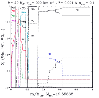
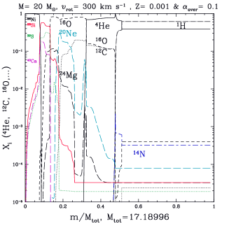
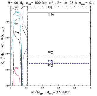
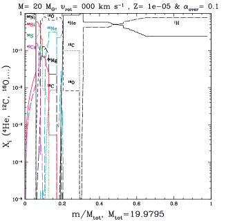
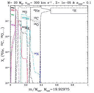
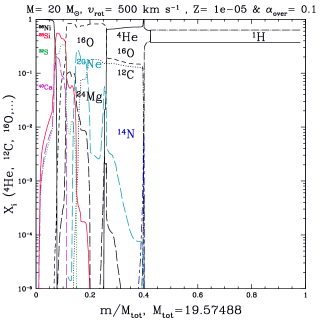
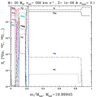
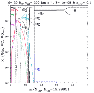
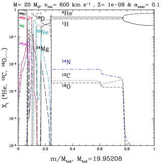
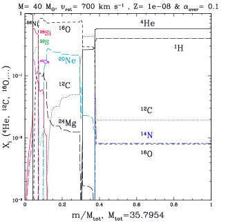
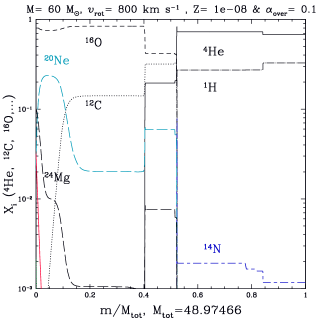
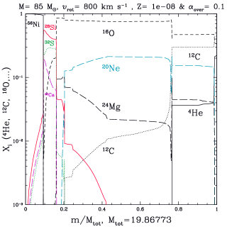
Figure 13: Final abundance profiles. The initial parameters of the models are given on top of each plot.

Precise measurements of surface abundances of extremely metal poor (EMP) stars have recently been obtained by Cayrel et al. (2004), Spite et al. (2005) and Israelian et al. (2004a). These provide new constraints for the stellar evolution models (see Chiappini et al., 2005; François et al., 2004; Prantzos, 2005). The most striking constraint is the need for primary ¹⁴N production in very low metallicity massive stars. Other constraints are an upturn of the [C/O] ratio with a [C/Fe] ratio (see for example Fig. 14 for C/O and Fig. 13 for C/Fe in Spite et al., 2005) about constant or slightly decreasing (with increasing metallicity) at very low metallicities, which requires an increase (with increasing metallicity) of oxygen yields below [Fe/H]$\sim$ -3. About one quarter of EMP stars are carbon rich (C-rich EMP, CEMP stars). Ryan et al. (2005) and Beers & Christlieb (2005) propose a classification for these CEMP stars. They find two categories: about three quarter are main s–process enriched (Ba-rich) CEMP stars and one quarter are enriched with a weak component of s–process (Ba-normal). The two most metal poor stars known to date, HE1327-2326 (Frebel et al., 2005; Aoki et al., 2006) and HE 0107-5240 (Christlieb et al., 2004) are both CEMP stars. These stars are believed to have been enriched by only one to several stars and the yields of the models can therefore be compared to their observed abundances without the filter of a galactic chemical evolution model (GCE).

The evolution of low metallicity or metal free stars is not a new subject (see for example Chiosi, 1983; El Eid et al., 1983; Carr et al., 1984; Arnett, 1996). The observations cited above have however greatly increased the interest in very metal poor stars. There are many recent works studying the evolution of metal free (or almost) massive (Heger & Woosley, 2002; Limongi & Chieffi, 2005; Umeda & Nomoto, 2005; Meynet et al., 2006), intermediate mass (Siess et al., 2002; Herwig, 2004; Suda et al., 2004; Gil-Pons et al., 2005) and low mass (Picardi et al., 2004; Weiss et al., 2004) stars in an attempt to explain the origin of the surface abundances observed. In this work pre-supernova evolution models of rotating single stars were computed with metallicities ranging from solar metallicity down to $Z=10^{-8}$ to study the impact of rotation and to see which initial rotation velocities can lead to the chemical enrichments observed. In Sect. 2, the model physical ingredients and the calculations are presented. In Sect. 3, the evolution of the models is described. In Sect. 4, the stellar yields of light elements are presented and compared to observations. In Sect. 5, the conclusions are given.

2 Description of the stellar models

The stellar evolution model used to calculate the stellar models is described in detail in Hirschi et al. (2004). Convective stability is determined by the Schwarzschild criterion. Convection is treated no longer as an instantaneous mixing but as a diffusive process from oxygen burning onwards. The overshooting parameter is 0.1 H_P for H and He–burning cores and 0 otherwise. The reaction rates are taken from the NACRE (Angulo et al., 1999) compilation for the experimental rates and from the NACRE website (http://pntpm.ulb.ac.be/nacre.htm) for the theoretical ones.

2.1 Initial composition

The initial composition of the models is given in Table 1. The solar metallicity composition is described in Hirschi et al. (2005b) and only low metallicity compositions are presented here. For a given metallicity $Z$ (in mass fraction), the initial helium mass fraction $Y$ is given by the relation $Y=Y_{p}+\Delta Y/\Delta Z\cdot Z$, where $Y_{p}$ is the primordial helium abundance and $\Delta Y/\Delta Z$ the slope of the helium–to–metal enrichment law. $Y_{p}$ = 0.24 and $\Delta Y/\Delta Z$ = 2.5 were used according to recent determinations (see Izotov & Thuan, 2004, for example). For the mixture of the heavy elements, the same mixture as the one used to compute the opacity tables for Weiss 95’s alpha–enriched composition (Iglesias & Rogers, 1996) was adopted.

Table 1: Initial abundance (in mass fraction) of the chemical elements followed in the calculations.

Element	$Z=10^{-3}$	$Z=10^{-5}$	$Z=10^{-8}$
1H	7.5650D-01	0.759965	0.759999965
3He	2.5702D-05	2.5440D-05	2.5437D-05
4He	2.4247D-01	0.23999956	0.239974588
12C	7.5542D-05	7.5542D-07	7.5542D-10
13C	9.0930D-07	9.0930D-09	9.0930D-12
14N	2.3358D-05	2.3358D-07	2.3358D-10
15N	9.2242D-08	9.2242D-10	9.2242D-13
16O	6.7105D-04	6.7105D-06	6.7105D-09
17O	2.7196D-07	2.7196D-09	2.7196D-12
18O	1.5162D-06	1.5162D-08	1.5162D-11
20Ne	7.8366D-05	7.8366D-07	7.8366D-10
22Ne	6.3035D-06	6.3035D-08	6.3035D-11
24Mg	3.2475D-05	3.2475D-07	3.2475D-10
25Mg	4.2685D-06	4.2685D-08	4.2685D-11
26Mg	4.8956D-06	4.8956D-08	4.8956D-11
28Si	3.2769D-05	3.2769D-07	3.2769D-10
32S	1.8897D-05	1.8897D-07	1.8897D-10
36Ar	1.9797D-06	1.9797D-08	1.9797D-11
40Ca	5.1728D-06	5.1728D-08	5.1728D-11
44Ti	0	0	0
48Cr	0	0	0
52Fe	0	0	0
56Ni	0	0	0

2.2 Mass loss

Since mass loss rates are a key ingredient for the evolution of massive stars, the prescriptions used are summarised here. The changes of the mass loss rates, $\dot{M}$, with rotation are taken into account as explained in Maeder & Meynet (2000a). As reference mass loss rates, the adopted mass loss rates are the ones of Vink et al. (2000, 2001), who account for the occurrence of bi–stability limits, which change the wind properties and mass loss rates. For the domain not covered by these authors the empirical law devised by de Jager et al. (1988) was used. Note that this empirical law, which presents a discontinuity in the mass flux near the Humphreys–Davidson limit, implicitly accounts for the mass loss rates of LBV stars. For the non–rotating models, since the empirical values for the mass loss rates are based on stars covering the whole range of rotational velocities, one must apply a reduction factor to the empirical rates to make them correspond to the non–rotating case. The same reduction factor was used as in Maeder & Meynet (2001). During the Wolf–Rayet phase the mass loss rates by Nugis & Lamers (2000) were used. The mass loss rates depend on metallicity as $\dot{M}\sim(Z/Z_{\odot})^{0.5}$, where $Z$ is the mass fraction of heavy elements at the surface of the star.

The mass loss rates (and opacity) are rather well determined for chemical compositions which are similar to solar composition or similar to a fraction of the solar composition (or of the alpha–enriched mixing). However, very little was known about the mass loss of very low metallicity stars with a strong enrichment in CNO elements until recently. Vink & de Koter (2005) study the case of WR stars and find a clear dependence with iron group mass fractions. For red supergiant stars (RSG), recent studies (see van Loon, 2005, and references therein) show that dust–driven winds at cool temperature show no metallicity dependence for $Z>0.1\,Z_{\odot}$. As we shall see later, due to rotational and convective mixing, the surface of the star is strongly enriched in CNO elements during the RSG stage. It is implicitly assumed in this work (as in Meynet et al., 2006) that CNO elements have a significant contribution to opacity and mass loss rates. The mass loss rates used depend on metallicity as $\dot{M}\sim(Z/Z_{\odot})^{0.5}$, where $Z$ is the mass fraction of heavy elements at the surface of the star, also when the iron group elements content is much lower than the CNO elements content. The largest mass losses in the present calculations occur during the RSG stage. This means that if the independence of the mass loss rates on the metallicity in the RSG stage (van Loon, 2005) is confirmed at very low metallicities, the mass loss rate used in this work possibly underestimate the real mass loss rate. This point surely deserves to be studied in more detail in the future.

A specific treatment for mass loss was applied at break-up (see Meynet et al., 2006). At break-up, the mass loss rate adjusts itself in such a way that an equilibrium is reached between the two following opposite effects. 1) The radial inflation due to evolution, combined with the growth of the surface velocity due to the internal coupling by meridional circulation, brings the star to break-up, and thus some amount of mass at the surface is no longer bound to the star. 2) By removing the most external layers, mass loss brings the stellar surface down to a level in the star that is no longer critical. Thus, at break-up, one should adapt the mass loss rates, in order to maintain the surface layers at the break-up limit. In practise, however, since the critical limit contains mathematical singularities, it was considered that during the break-up phase, the mass loss rates should be such that the model stays near a constant fraction (around 0.95) of the limit. Note that wind anisotropy (described in Maeder & Meynet, 2000a) was not taken into account for the present work.

2.3 Chemical elements and angular momentum transport

The instabilities induced by rotation taken into account in this work are meridional circulation and secular and dynamical shears. Meridional circulation is an advective process and shears are diffusive processes. The equations for the transport of angular momentum and chemical elements are given in Sect. 2.3 of Maeder & Meynet (2000b). For more details on the equation for the transport of angular momentum, the reader can refer to Maeder & Zahn (1998). The equation for the change of the mass fraction of chemical species $i$ is the following:

$$\left(\frac{dX_{i}}{dt}\right)_{M_{r}}=\left(\frac{\partial}{\partial M_{r}}\right)_{t}\left[(4\pi r^{2}\rho)^{2}D\left(\frac{\partial X_{i}}{\partial M_{r}}\right)_{t}\right]+\left(\frac{dX_{i}}{dt}\right)_{\rm n}$$ (1)

The second term on the right accounts for composition changes due to nuclear reactions. Note that the nuclear burning term and the diffusive term are treated in a serial way in the simulations. The coefficient $D$ is the sum of the different diffusion coefficients: $D=D_{\rm conv}+D_{\rm eff}+D_{\rm shear}$, where $D_{\rm conv}$ is the convective diffusion coefficient, $D_{\rm eff}$ accounts for the combined effect of advection and horizontal turbulence and $D_{\rm shear}$ represents the sum of secular (see Eqs. 5.32 in Maeder, 1997) and dynamical (see Eq. 5 in Hirschi et al., 2004) shear coefficients. Although meridional circulation is an advective process, its effect on the change in chemical abundances can be approximated by a diffusion process. The coefficient $D_{\rm eff}$ (accounting for the combined effect of advection and horizontal turbulence) is calculated in this work using the following formula:

$$D_{\rm eff}=\frac{\mid rU(r)\mid^{2}}{30D_{h}}\;,$$ (2)

where $D_{h}$ is the coefficient of horizontal turbulence, for which the estimate is $D_{h}=|rU(r)|$ (Zahn, 1992). This equation expresses that the vertical advection of chemical elements is severely inhibited by the strong horizontal turbulence characterised by $D_{h}$.

Even though there is no free parameter in the prescriptions above to increase or decrease the importance of the coefficients, different authors use different prescriptions for the various processes (see for example Heger et al., 2000). The coefficient of horizontal turbulence was also recently revised (Maeder, 2003). The new coefficient was used in Meynet et al. (2006) but not in this work. The impact of the new coefficient is discussed briefly in Sect. 3.4.

2.4 Initial rotation

The value of 300 km s^-1 as the initial rotation velocity at solar metallicity corresponds to an average velocity of about 220 km s^-1 on the Main Sequence (MS) which is very close to the average observed value (see for instance Fukuda, 1982). It is unfortunately not possible to measure the rotational velocity of very low metallicity massive stars since they all died a long time ago. Higher observed ratio of Be to B stars in the Magellanic clouds compared to our Galaxy (Maeder et al., 1999) could point out to the fact the stars rotate faster at lower metallicities. Also a low metallicity star containing the same angular momentum as a solar metallicity star has a higher surface rotation velocity due to its smaller radius (one quarter of $Z_{\odot}$ radius for 20 $M_{\odot}$ stars). Since there is however not yet firm evidence for fast surface rotation velocities at low metallicities, we explore in this work with 20 $M_{\odot}$ models different velocities ranging between no rotation and surface velocities corresponding to the same total angular momentum as in solar metallicity stars.

In order to compare the models at different metallicities and with different initial masses with another quantity than the surface velocity, the ratio $\upsilon_{\rm ini}/\upsilon_{\rm crit}$ is used (see Table 2). The critical velocity is reached when the gravitational acceleration is balanced by radiative and centrifugal forces. The critical velocity is given by the following formula if the star is far from its Eddington limit ($\Gamma_{\rm max}<0.64$):

$$v_{\mathrm{crit,1}}=\Omega\;R_{\mathrm{eb}}=\left(\frac{2}{3}\frac{GM}{R_{\mathrm{pb}}}\right)^{\frac{1}{2}}\;.$$ (3)

$R_{\mathrm{eb}}$ and $R_{\mathrm{pb}}$ are respectively the equatorial and polar radius at the break–up velocity. If the star gets closer to the Eddington limit, then the following critical velocity has to be used:

$$v_{\mathrm{crit,2}}^{2}=\frac{9}{4}\;v_{\mathrm{crit,1}}^{2}\;\frac{1-\Gamma_{\mathrm{max}}}{V^{\prime}(\omega)}\;\frac{R^{2}_{\mathrm{e}}(\omega)}{R^{2}_{\mathrm{pb}}}\;,$$ (4)

where R${}_{\mathrm{e}}(\omega)$ is the equatorial radius for a given value of the rotation parameter $\omega$. More details can be found in Maeder & Meynet (2000a). Towards lower metallicities, $\upsilon_{\rm ini}/\upsilon_{\rm crit}$ increases only as $r^{-1/2}$ for models with the same angular momentum ($J$), whereas the surface rotational velocity increases as $r^{-1}$ ($J\sim\upsilon r$). The angular momentum varies significantly for models with different initial masses. Finally, $\upsilon_{\rm ini}/\upsilon_{\rm crit}$ is a good indicator for the impact of rotation on mass loss.

In the first series of models, the aim is to scan the parameter space of rotation and metallicity with 20 $M_{\odot}$ models since a 20 $M_{\odot}$ star is not far from the average massive star when a Salpeter (1955) like IMF is used. For this series, on top of non-rotating models, two initial rotational velocities were used at very low metallicities. The first velocity is the same as at solar metallicity, i. e. 300 km s^-1. The ratio $\upsilon_{\rm ini}/\upsilon_{\rm crit}$ decreases with metallicity (see Table 2) for the initial velocity of 300 km s^-1. The second $\upsilon_{\rm ini}$ is 500 km s^-1 at Z=10^-5 ([Fe/H]$\sim$-3.6) and 600 km s^-1 at Z=10^-8 ([Fe/H]$\sim$-6.6). These values have ratios of the initial velocity to the break–up velocity, $\upsilon_{\rm ini}/\upsilon_{\rm crit}$ around 0.55, which is only slightly larger than the solar metallicity value (0.44). The 20 $M_{\odot}$ model at Z=10^-8 and with 600 km s^-1 has a total initial angular momentum $J_{\rm tot}=3.3\,10^{52}$ erg s, which is the same as for the solar metallicity 20 $M_{\odot}$ model with 300 km s^-1 ($J_{\rm tot}=3.6\,10^{52}$ erg s). So even though a star at Z=10^-8 with a velocity of 600 km s^-1 at first glance seems to be an extremely fast rotator, it is in fact similar to a solar metallicity star in terms of angular momentum and ratio $\upsilon_{\rm ini}/\upsilon_{\rm crit}$. In the second series of models, following the work of Meynet et al. (2006), models were computed at Z=10^-8 with initial masses of 40, 60 and 85 $M_{\odot}$ and initial rotational velocities of 700, 800 and 800 km s^-1 respectively. Note that, for these models as well, the initial total angular momentum is similar to the one contained in solar metallicity models with rotational velocities equal to 300 km s^-1.

Table 2: Initial parameters of the models (columns 1–5): mass, metallicity, rotation velocity [km s^-1], total angular momentum [$10^{53}$ erg s] and $\upsilon_{\rm ini}/\upsilon_{\rm crit}$. Lifetimes [Myr] (6–8): total and core hydrogen and helium burnings. Various masses [$M_{\odot}$] (9–14): final mass, masses of the helium, carbon–oxygen, silicon and iron cores and the remnant mass.

$M_{\rm{ini}}$	$Z_{\rm{ini}}$	$\upsilon_{\rm{ini}}$	$J_{\rm{tot}}^{\rm{ini}}$	$\upsilon_{\rm ini}/\upsilon_{\rm crit}$	$\tau_{\rm{life}}$	$\tau_{\rm{H}}$	$\tau_{\rm{He}}$	$M_{\rm{final}}$	$M_{\alpha}$	$M_{\rm{CO}}$	$M_{\rm{Si}}$	$M_{\rm{Fe}}$	$M_{\rm{rem}}^{a}$
20	2e-2	300	0.36	0.44	11.0	10.1	0.798	8.7626	8.66	6.59	2.25	1.27	2.57
20	1e-3	000	–	0.00	10.0	9.02	0.875	19.5567	6.58	4.39	1.75	1.16	2.01
20	1e-3	300	0.34	0.39	11.5	10.6	0.813	17.1900	8.32	6.24	2.27	1.33	2.48
20	1e-5	000	–	0.00	9.80	8.86	0.829	19.9795	6.24	4.28	1.67	1.18	1.98
20	1e-5	300	0.27	0.34	11.1	10.2	0.806	19.9297	7.90	5.68	1.99	1.30	2.34
20	1e-5	500	0.42	0.57	11.6	10.6	0.812	19.5749	7.85	5.91	2.18	1.35	2.39
20	1e-8	000	–	0.00	8.96	8.24	0.598	19.9994	4.43	4.05	1.91	1.05	1.92
20	1e-8	300	0.18	0.28	9.98	9.20	0.610	19.9992	6.17	5.18	1.96	1.29	2.21
20	1e-8	600	0.33	0.55	10.6	9.71	0.703	19.9521	4.83	4.36	2.01	1.29	2.00
09	1e-8	500	0.80	0.08	30.5	26.8	3.24	8.9995	1.90	1.34	–	–	1.21
40	1e-8	700	1.15	0.55	5.77	5.31	0.402	35.7954	13.5	12.8	2.56	1.49	4.04
60	1e-8	800	2.41	0.57	4.55	4.19	0.321	48.9747	25.6	24.0	–	–	7.38
85	1e-8	800	4.15	0.53	3.86	3.50	0.322	19.8677	19.9	18.8	3.19	1.84	5.79

^a estimated from the CO core mass.

3 Evolution

The evolution of the models was in general followed until core Si–burning. The 60 $M_{\odot}$ model was evolved until neon burning and the 9 $M_{\odot}$ model until carbon burning. The main characteristics of the models are presented in Table 2.

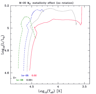
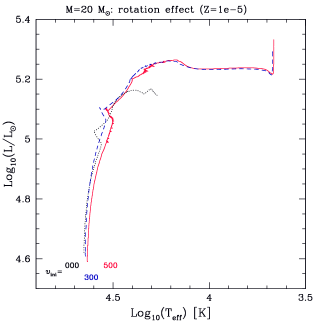
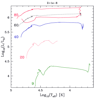
Figure 1: HR diagrams: (left) non–rotating 20 $M_{\odot}$ models, (middle) 20 $M_{\odot}$ models with $Z=10^{-5}$ and (right) $Z=10^{-8}$ models with average rotation.

3.1 Metallicity effects

The effects of metallicity on stellar evolution have already been discussed in the literature (see for example Heger et al., 2003; Chieffi & Limongi, 2004; Meynet et al., 1994). But before looking at the very low metallicity models and the impact of rotation, it is useful to summarise the effects low metallicity has on the evolution of massive stars. A lower metallicity implies a lower luminosity which leads to slightly smaller convective cores. This can be seen in Table 2 by comparing the core masses of non–rotating the 20 $M_{\odot}$ models at different metallicities. A lower metallicity implies lower opacity and lower mass losses (as long as the chemical composition has not been changed by burning or mixing in the part of the star one considers). So at the start of the evolution lower metallicity stars are more compact. This can be seen in the Herzsprung–Russell (HR) diagram (Fig. 1 left) where the lower metallicity models have bluer tracks during the main sequence. They also lose less mass as can be seen by looking at the final masses in Table 2. The lower metallicity models also have a harder time reaching the red supergiant (RSG) stage (see Maeder & Meynet, 2001, for a detailed discussion). The non–rotating model at $Z=10^{-3}$ becomes a RSG only during shell He–burning (see Fig. 2) and the lower metallicity non–rotating models never reach the RSG stage. As long as the metallicity is above about $Z=10^{-10}$, no significant differences have been found in non–rotating models. Below this metallicity and for metal free stars, the CNO cycle cannot operate at the start of H–burning. At the end of its formation, the star therefore contracts until it starts He-burning because the pp–chains cannot balance the effect of the gravitational force. Once enough carbon and oxygen are produced, the CNO cycle can operate and the star behaves like stars with $Z>10^{-10}$ for the rest of the main sequence. Shell H–burning still differs between $Z>10^{-10}$ and metal free stars. Metal free stellar models are presented in Chieffi & Limongi (2004), Heger & Woosley (2002) and Umeda & Nomoto (2005).

3.2 Rotation effects

How does rotation change this picture? At all metallicities, rotation usually increases the core sizes, the lifetimes, the luminosity and the mass loss. Maeder & Meynet (2001) and Meynet & Maeder (2002) have already studied the impact of rotation down to a metallicity of $Z=10^{-5}$. They find in Maeder & Meynet (2001) that rotation favours a redward evolution and that rotating models can reproduce the observed ratio of blue to red supergiants (B/R) in the small Magellanic cloud. We can see in Fig. 1 (middle) that the rotating models at $Z=10^{-5}$ become RSGs during shell He–burning (See Fig. 2). This does not change the ratio B/R but changes the structure of the star when the SN explodes. At $Z=10^{-8}$ (Fig. 1 right), the 20 $M_{\odot}$ models do not become RSG. However other mass models do reach the RSG stage and the 85 $M_{\odot}$ model even becomes a WR star of type WO (see below). Maeder & Meynet (2001) also find that a larger fraction of stars reach break-up velocities during the evolution. This will be further discussed in Sect. 3.4).

In Meynet & Maeder (2002), they show that low metallicity ($Z=10^{-5}$) models have strong internal $\Omega$–gradients, which favours an important mixing. This mixing leads to primary nitrogen production during He–burning by rotational diffusion of carbon and oxygen into the H-burning shell. Their results already point out that the primary nitrogen yields strongly depend on the initial rotation velocity. This dependence is further studied in Sect. 4.

Meynet et al. (2006) present the evolution of 60 $M_{\odot}$ models at $Z=10^{-8}$ and confirm the effects that were predicted in their previous papers. The fast rotating model, with an initial rotational velocity of 800 km s^-1 reaches break-up, becomes a red supergiant and produces significant amount of primary nitrogen. The model becomes a Wolf–Rayet (WR) star due to large mass losses during the RSG stage. These effects are further discussed below and models at $Z=10^{-8}$ with different initial masses are presented.

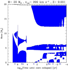
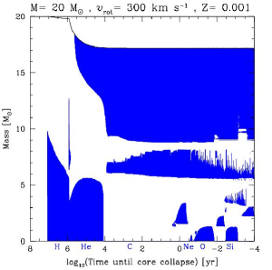
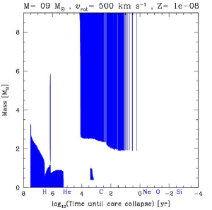
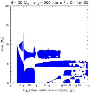
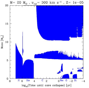
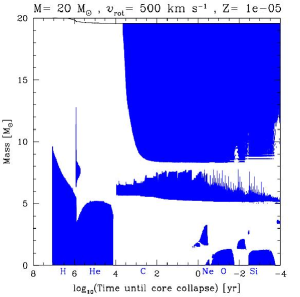
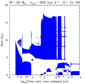
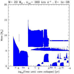
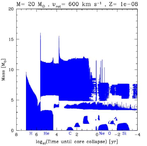
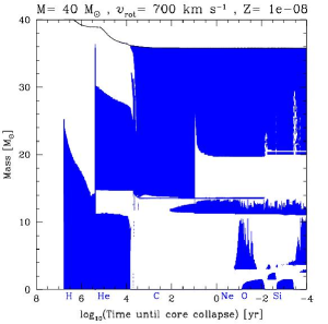
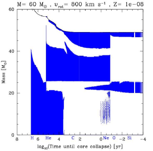
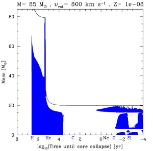
Figure 2: Stellar structure (Kippenhahn) diagrams, which show the evolution of the structure as a function of the time left until the core collapse. The initial parameters of the models are given on top of each plot. The coloured zone correspond to the convective zones and the symbols of the burning stages are given below the time axis.

3.3 Strong impact of mixing at very low metallicities

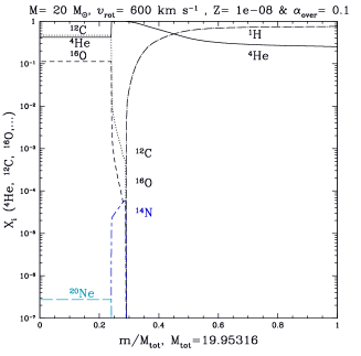
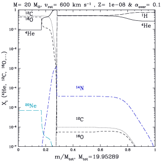
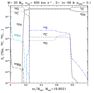
Figure 12: Abundance profiles for the 20 $M_{\odot}$ with $\upsilon_{\rm ini}=$600 km s^-1 at $Z=10^{-8}$: (left) before shell H–burning boost (induced by mixing of carbon and oxygen from the core), (middle) just after the boost and (right) after shell H–burning has deepened during shell He–burning.

At solar metallicity and metallicities higher than about $Z=10^{-5}$, rotational mixing increases the helium and CO core masses (see Table 2). In particular, the oxygen yield is increased. The impact of mixing on models at $Z=10^{-8}$ (and at $Z=0$ see Ekström et al., 2006) is however different for fast rotation ($\upsilon_{\rm ini}=$600-800 km s^-1). The impact of mixing on the structure and convective zones is represented in the Kippenhahn diagram for the $Z=10^{-8}$ models (see Fig. 2). During hydrogen burning and the start of helium burning, the impact of mixing is the same as at higher metallicity: mixing increases the core sizes and mixing of helium above the core suppresses the intermediate convective zones linked to shell H–burning. The difference from higher metallicity models occurs during He–burning. As shown in Fig. 12 (left) for the 20 $M_{\odot}$ with $\upsilon_{\rm ini}=$600 km s^-1, primary carbon and oxygen are mixed outside of the convective core into the H–burning shell. Once the enrichment is strong enough, the H–burning shell is boosted (the CNO cycle depends strongly on the carbon and oxygen mixing at such low initial metallicities). The shell then becomes convective, as can be seen in Fig. 3, which is a zoom of the Kippenhahn diagram. The boost phase, which could look like an instantaneous event in Fig. 2 (third line, right), is fully revealed in this zoom. The calculations have been repeated with different time steps to verify that the results did not depend on the numerical details. The evolution of the final model was followed with 2000 time steps between the time axis measures of 5.607 and 5.596.

In response to the shell boost, the core expands and the convective core mass decreases. At the end of He–burning, the CO core is less massive than in the non–rotating model (Fig. 2, third line, left and right). The yield of ¹⁶O being closely correlated with the mass of the CO core, it is therefore reduced due to the strong mixing. At the same time the carbon yield is slightly increased (See Table 3). It is interesting to note that the shell H–burning boost occurs in all the different initial mass models at $Z=10^{-8}$ as can be seen in Fig. 2 (noticeable by the appearance of a strong intermediate convective shell due to H–burning and the corresponding sharp decrease in the He–burning convective core mass). This means that the relatively ”low” oxygen yields and ”high” carbon yields are produced over a large mass range at $Z=10^{-8}$. This could be an explanation for the possible high [C/O] ratio observed in the most metal poor halo stars (ratio between the surface abundances of carbon and oxygen relative to solar; see Fig. 14 in Spite et al., 2005).

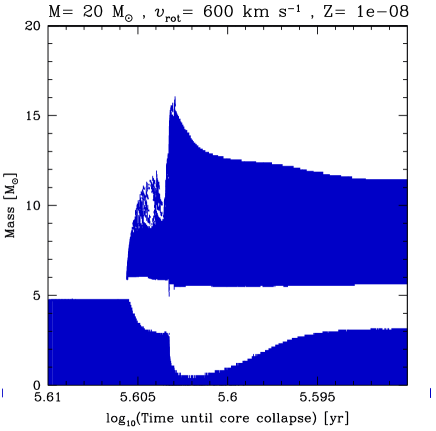
Figure 3: Stellar structure (Kippenhahn) diagram of the 20 $M_{\odot}$ with $\upsilon_{\rm ini}=$600 km s^-1 at $Z=10^{-8}$. The central convective zone is created by core He–burning and the intermediate convective zone is created by shell H–burning. This is a zoom around the time when the shell H–burning is boosted due to strong mixing of carbon and oxygen from the core. The graph shows the apparition of the convective zone induced by shell H–burning and that the mass of the helium burning core is smaller after than before the H–burning shell boost.

Figure 12 (left) shows the abundance profiles before the shell H–burning boost and Fig. 12 (middle) shows the profiles after. These profiles show that the carbon and oxygen brought to the shell H–burning are transformed into primary nitrogen. The bulk of primary nitrogen is however produced later in the evolution. It happens when the shell H–burning deepens in mass during core helium burning for the very massive models and during shell He–burning for the 20 $M_{\odot}$ model. The deepening of the convective H–burning shell is caused by dynamical shear instabilities (see Sect. 2.3 in Hirschi et al., 2004, and references therein). Dynamical shear instabilities take place just below the bottom of the convective zone due to the strong differential rotation between the convective H–burning shell and the layers below (deeper in the star). Dynamical shear instabilities occur on a dynamical time scale as opposed to secular shear and they therefore induce a fast mixing just below the convective zone. Note that the dynamical shear instabilities are not influenced by mean molecular weight gradients. The consequences are the same as during the first boost. Carbon and oxygen are mixed inside the H–burning shell and a new boost occurs, producing this time more nitrogen because the newly mixed material is richer in carbon and oxygen. Figure 12 (right) shows the abundance profiles after the second boost. The abundance of nitrogen does not change later during the advanced stages and the pre–SN profile for nitrogen (see Fig. 13) stays the same. The total production of primary nitrogen is further discussed in Sect. 4. Rotational mixing also influences strongly the mass loss of very massive stars as is discussed below.

3.4 Mass loss

Mass loss becomes gradually unimportant as the metallicity decreases in the 20 $M_{\odot}$ models. At solar metallicity, the rotating 20 $M_{\odot}$ model loses more than half of its mass, at $Z=0.001$, the models lose less than 15% of their mass, at $Z=10^{-5}$ less than 3% and at $Z=10^{-8}$ less than 0.3% (see Table 2). Meynet et al. (2006) show that the situation can be very different for a 60 $M_{\odot}$ star at $Z=10^{-8}$. Indeed, their 60 $M_{\odot}$ model loses about half of its initial mass. About ten percents of the initial mass is lost when the surface of the star reaches break–up velocities during the main sequence. The largest mass loss occurs during the red supergiant (RSG) stage due to the mixing of primary carbon and oxygen from the core to the surface through convective and rotational mixing. The large mass loss is due to the fact that the star crosses the Humphreys-Davidson limit.

What happens in the models calculated in this study? First let us study the mass loss at break–up. Figure 4 presents the evolution of the surface velocity and of the ratio of the surface angular velocity to the critical angular velocity, $\Omega/\Omega_{\rm crit}$ for the 85 $M_{\odot}$ (red solid line), 40 $M_{\odot}$ (dotted black line) and 20 $M_{\odot}$ (dashed blue line) models with fast rotation velocities, $\upsilon_{\rm ini}=$600-800 km s^-1, at $Z=10^{-8}$. It shows that the 20 $M_{\odot}$ model only reaches break–up velocities at the end of the main sequence (MS) and therefore does not lose mass due to this phenomenon. However, more massive models reach critical velocities early during the MS (the earlier the more massive the model). The evolution of rotation for the 60 $M_{\odot}$ model is very similar to the 40 $M_{\odot}$ model and is therefore not shown here for the clarity of the plot. The mass lost due to break–up increases with the initial mass and amounts to 1.1, 3.5 and 5.5 $M_{\odot}$ for the 40, 60 and 85 $M_{\odot}$ models respectively (see the top solid line in Fig. 2 going down during the MS). At the end of core H–burning, the core contracts and the envelope expands, thus decreasing the surface velocity and $\Omega/\Omega_{\rm crit}$. The mass loss rates becomes very low again until the star crosses the HR diagram and reaches the RSG stage. At this point the convective envelope dredges up CNO elements to the surface increasing its overall metallicity. As said in Sect. 2.2, the total metallicity, $Z$, is used (including CNO elements) for the metallicity dependence of the mass loss. Therefore depending on how much CNO is brought up to the surface, the mass loss can become very large again. The CNO brought to the surface comes from primary C and O produced in He–burning. As described in the above subsection, rotational and convective mixing brings these elements into the H–burning shell. A large fraction of the C and O is then transformed into primary nitrogen via the CNO cycle. Additional convective and rotational mixing is necessary to bring the primary CNO to the surface of the star. The whole process is complex and depends on mixing (see Fig. 5).

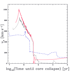
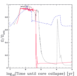
Figure 4: Evolution of rotation for the 85 $M_{\odot}$ (red solid line), 40 $M_{\odot}$ (dotted black line) and 20 $M_{\odot}$ (dashed blue line) models with fast rotation velocities, $\upsilon_{\rm ini}=$600-800 km s^-1, at $Z=10^{-8}$: (left) surface equatorial velocity, and (right) ratio of the surface angular velocity to the critical angular velocity, $\Omega/\Omega_{\rm crit}$.

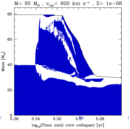
Figure 5: Stellar structure (Kippenhahn) diagram of the 85 $M_{\odot}$ model at $Z=10^{-8}$. This is a zoom covering the period when C and O are transported from the core to the surface and induce a strong mass loss. The central convective zone is related to core He–burning. The main intermediate convective zone is caused by shell H–burning and the surface convective zone appears when the star becomes a RSG.

Of particular importance is the surface convective zone, which appears when the star becomes a RSG. This convective zone dredges-up the CNO to the surface. For a very large mass loss to occur, it is necessary that the star becomes a RSG in order to develop a convective envelope. It is also important that the extent of the convective envelope is large enough to reach the CNO rich layers. Finally, the star must reach the RSG stage early enough (before the end of core He–burning) so that there will be time remaining to lose mass. Figure 6 shows the evolution of the effective temperature as a function of the central helium mass fraction. This figure shows that the 9 and 40 $M_{\odot}$ models reach the RSG stage only after the end of helium burning, so too late for a large mass loss. The 60 $M_{\odot}$ model reaches the RSG stage during He–burning. It would therefore have time to lose large amounts of mass. However, the dredge–up is not strong enough. The 85 $M_{\odot}$ model becomes a RSG during He–burning earlier than the 60 $M_{\odot}$ model. The dredge-up is stronger for this model and the surface CNO abundance becomes very high (see Fig. 8 bottom). The series of models presented here constrain the minimum initial mass for significant mass loss (more than half of the initial mass) to be between 60 and 85 $M_{\odot}$.

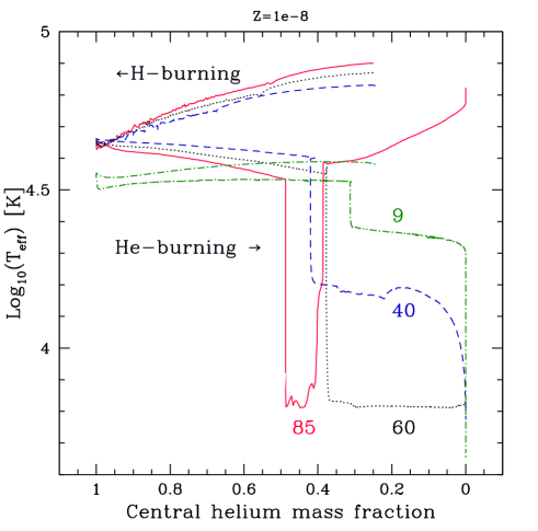
Figure 6: Evolution of the effective temperature as a function of the central helium mass fraction for the $Z=10^{-8}$ models. Models evolve from the top right corner to the top left corner during the MS. They then evolve to the right during helium burning and downwards when they become RSG. The 20 $M_{\odot}$ track resembles the 9 $M_{\odot}$ model track except that it doesn’t reach the RSG stage at the end of He–burning.

The dependence on mixing of the lower initial mass for a large mass loss to occur can be estimated by comparing the 60 $M_{\odot}$ model calculated here and the one presented by Meynet et al. (2006). The model calculated by Meynet et al. (2006), which does not include overshooting and uses a different prescription for the horizontal diffusion coefficient, $D_{\rm h}$ (Maeder, 2003), loses a large fraction of its mass (and becomes a WR star with high effective temperature) just before the end of core helium burning (see Fig. 4 from Meynet et al., 2006). The $D_{\rm h}$ used in Meynet et al. (2006), compared to the $D_{\rm h}$ used in the present calculations, tends to allow a larger enrichment of the surface in CNO processed elements. This different physical ingredient explains the differences between the two 60 $M_{\odot}$ models. The fact that, out of two 60 $M_{\odot}$ models, one model does not lose much mass and the other model with a different physics just does, could mean that the minimum initial mass for the star to lose a large fraction of its mass is around 60 $M_{\odot}$.

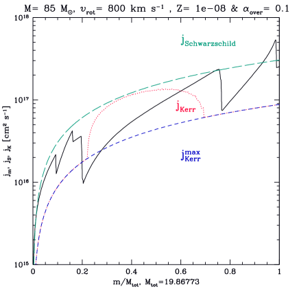
Figure 7: Profile of the specific angular momentum at the pre–SN stage for the 85 $M_{\odot}$ model at $Z=10^{-8}$ (solid line). The red dotted line shows the minimum angular momentum necessary in order to form an accretion disk around a rotating black hole. The blue short dashed and green long dashed lines show the minimum angular momentum necessary for a maximally rotating and a non–rotating black hole respectively.

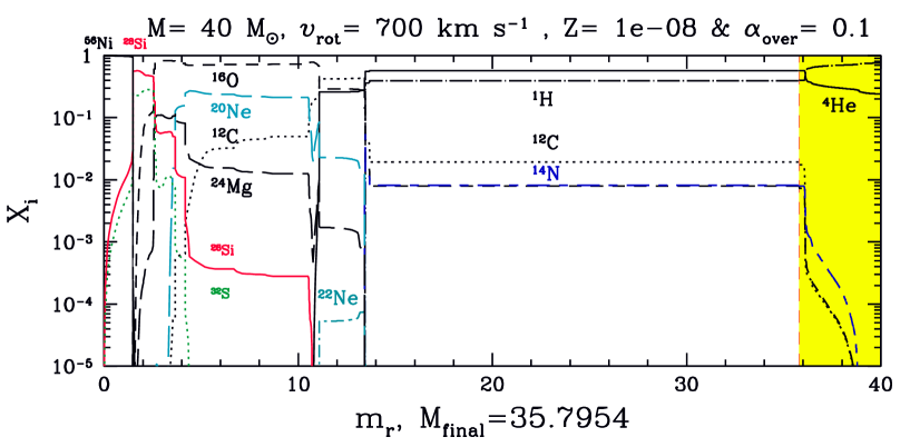
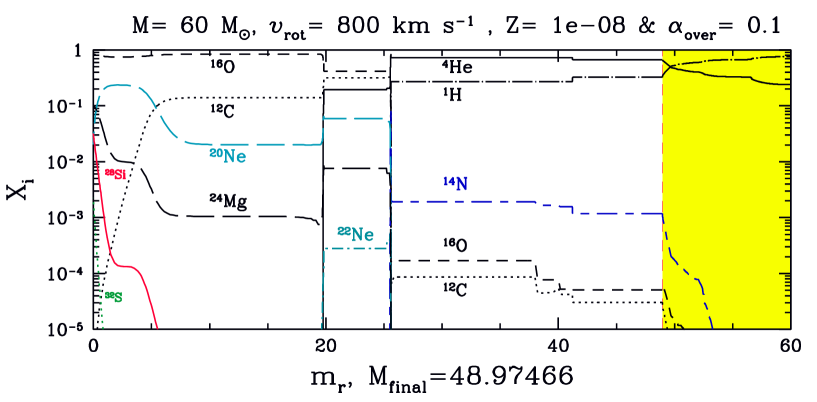
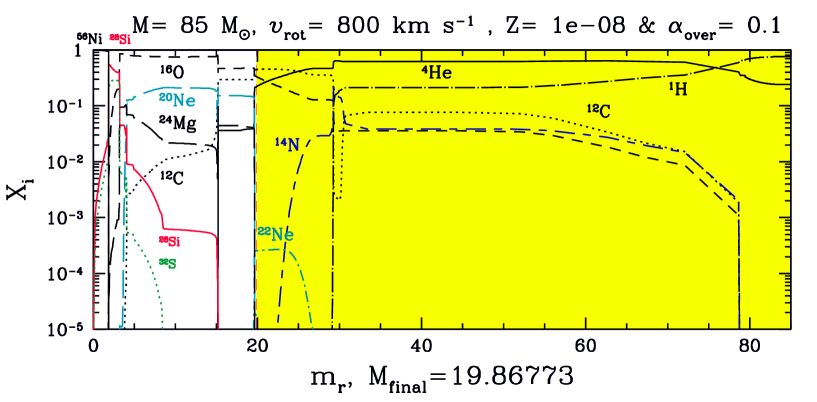
Figure 8: Abundance profiles for the 40 (top), 60 (middle) and 85 (bottom) $M_{\odot}$ models. The pre–SN and wind (yellow shaded area) chemical compositions are separated by a red dashed line located at the pre–SN total mass ($M_{\rm final}$), given below each plot.

Table 3: Initial mass, metallicity and velocity and total stellar yields^a ($mp^{\rm{pre-SN}}_{im}+mp^{\rm{wind}}_{im}$) of the models. All masses and yields are in solar mass units and velocities are in km s^-1. For the metallicity, $Z_{\rm{ini}}$ is in log10 units (-3 corresponds to $Z_{\rm{ini}}=10^{-3}$) except for $Z=0.02$ ($\odot$). Z is the total metal content and is defined by: Z$=1-X_{\rm{{}^{1}H}}-X_{\rm{{}^{3}He}}-X_{\rm{{}^{4}He}}$. These are the yields to be used for chemical evolution models using Eq. 2 from (Maeder, 1992).

$M$	$Z_{\rm{ini}}$	$\upsilon_{\rm{ini}}$	4He	$\rm\frac{{}^{3}He}{10^{4}}$	12C	13C	14N	16O	17O	18O	22Ne	$Z$
20	$\odot$	300	1.62	-3.36	0.433	1.01e-3	4.33e-2	2.57	-2.75e-6	-1.96e-4	4.26e-2	3.98
20	-3	000	2.47	-2.84	0.373	2.58e-5	3.31e-3	1.46	-5.48e-7	-1.12e-5	2.48e-3	2.38
20	-3	300	2.11	-3.31	0.676	2.84e-5	3.10e-3	2.70	4.83e-7	-1.89e-5	1.04e-2	3.77
20	-5	000	2.50	-3.32	0.370	1.93e-7	4.27e-5	1.50	3.05e-7	-9.43e-8	2.11e-5	2.30
20	-5	300	2.34	-3.91	0.481	2.42e-6	1.51e-4	2.37	3.40e-7	5.27e-7	2.74e-3	3.35
20	-5	500	2.26	-4.08	0.648	1.53e-5	5.31e-4	2.59	4.79e-7	5.49e-6	1.07e-2	3.54
20	-8	000	2.27	-4.17	0.262	2.27e-4	8.52e-3	1.20	1.94e-7	-2.15e-0	1.85e-6	2.14
20	-8	300	2.03	-4.37	0.381	1.80e-6	1.20e-4	1.96	1.70e-8	2.14e-7	5.48e-5	2.97
20	-8	600	3.15	-4.50	0.823	5.55e-3	5.90e-2	1.35	1.73e-5	2.52e-7	7.72e-5	2.49
09	-8	500	1.43	-1.76	0.082	1.35e-4	2.53e-3	5.85	5.64e-7	4.07e-5	1.86e-4	0.143
40	-8	700	6.01	-9.10	1.79	6.31e-2	1.87e-1	5.94	6.31e-5	4.74e-7	1.51e-4	9.64
60	-8	800	8.97	-13.3	3.58	5.00e-4	4.14e-2	12.8	6.26e-6	3.56e-7	1.66e-3	17.1
85	-8	800	16.8	-2.00	7.89	5.60e-1	1.75e+0	12.3	6.66e-4	4.95e-5	1.55e-3	25.5

^a Note that the corresponding ejected masses can be calculated by adding the initial composition given in Table 1 multiplied by the mass interval, the mass boundaries of which (initial and remnant masses) are given in Table 2.

Table 4: Initial mass and velocity and stellar wind yields^a ($mp^{\rm{wind}}_{im}$) of the $Z=10^{-8}$ models. All masses and yields are in solar mass units and velocities are in km s^-1.

$M$	$\upsilon_{\rm{ini}}$	4He	3He	12C	13C	14N	16O	17O	18O	22Ne	$Z$
09	500	2.80e-5	-8.34e-9	5.86e-08	1.72e-09	2.53e-08	2.33e-08	6.19e-12	1.20e-11	9.77e-12	1.10e-7
20	600	2.36e-4	-1.04e-6	-3.27e-11	5.06e-13	3.08e-10	-2.54e-10	5.30e-13	-7.22e-13	2.72e-16	7.59e-9
40	700	3.29e-1	-1.03e-4	5.34e-03	8.06e-04	3.63e-03	2.42e-03	1.05e-06	2.18e-09	2.35e-07	1.17e-2
60	800	1.21e+0	-2.72e-4	1.80e-05	4.94e-06	6.87e-04	5.48e-05	7.94e-08	-9.49e-11	4.80e-08	7.25e-4
85	800	2.00e+1	-1.64e-3	6.34e+00	5.60e-01	1.75e+00	3.02e+00	6.66e-04	4.95e-05	1.46e-03	1.16e+1

^a Note that the corresponding ejected masses can be calculated by adding the initial composition given in Table 1 multiplied by the mass interval, the mass boundaries of which (initial and final masses) are given in Table 2. For heavy elements with yields larger than 1e-6, ejected masses and stellar yields are essentially the same here since the initial total metallicity is 1e-8.

3.5 WR stars at very low metallicities

The lower limit for WR star formation is roughly the same as for large mass loss to occur, i.e. probably about 60 $M_{\odot}$, since models calculated here that lose a lot of mass become WRs. Therefore our models of single rotating massive stars produce WR stars at very low metallicities. The 85 $M_{\odot}$ model even becomes a WO type WR star. SNe of type Ib and Ic are therefore predicted to ensue from the death of single massive stars at very low metallicities. The next question is whether or not these stars can produce long and soft gamma ray bursts (GRBs) via the collapsar model (Woosley, 1993). Figure 7 shows the angular momentum distribution at the pre–SN stage. This figure shows that the core has enough angular momentum to produce a GRB (see Yoon & Langer, 2005; Woosley & Heger, 2006; Hirschi et al., 2005a, for more details on GRB progenitors). The effects of magnetic fields are however not included in the calculations. It is therefore possible that the core will not retain enough angular momentum to form an accretion disk. It is interesting to point out here that the outer part of the star also contains sufficient angular momentum to form an accretion disk, which is less likely to be removed due to the effects of magnetic fields. In a very optimistic outcome, one could imagine that the model could produce two jet episodes, one when the core collapses and one when the outer parts collapse, since for such a high initial mass the central black hole could swallow the whole pre–SN structure.

4 Stellar yields of light elements and comparison with observations

4.1 Stellar yields

The stellar yields are calculated using the same formulae as in Hirschi et al. (2005b). The wind contribution from a star of initial mass, $m$, to the stellar yield of an element $i$ is:

$$mp^{\rm{wind}}_{im}=\int_{0}^{\tau(m)}\dot{M}(m,t)[X_{i}^{S}(m,t)-X_{i}^{0}]\,dt$$ (5)

where $\tau(m)$ is the final age of the star, $\dot{M}(m,t)$ the mass loss rate when the age of the star is equal to $t$, $X_{i}^{S}(m,t)$ the surface abundance in mass fraction of element $i$ and $X_{i}^{0}$ its initial mass fraction (see Table 1). The pre–SN contribution from a star of initial mass, $m$, to the stellar yield of an element $i$ is:

$$mp^{\rm{pre-SN}}_{im}=\int_{m(\rm{rem})}^{m(\tau)}[X_{i}(m_{r})-X_{i}^{0}]\,dm_{r}$$ (6)

where $m(\rm{rem})$ is the remnant mass estimated from the CO core mass (see Maeder, 1992), $m(\tau)$ the final stellar mass, $X_{i}^{0}$ the initial abundance in mass fraction of element $i$ and $X_{i}(m_{r})$ the final abundance in mass fraction at the lagrangian mass coordinate, $m_{r}$. The pre–SN contribution is calculated at the end of Si–burning. Therefore the contribution from explosive nucleosynthesis is not included. However, elements lighter than neon are marginally modified by explosive nucleosynthesis (Chieffi & Limongi, 2003; Thielemann et al., 1996) and are mainly determined by the hydrostatic evolution. The total stellar yield of an element $i$ from a star of initial mass, $m$, is then :

$$mp^{\rm{tot}}_{im}=mp^{\rm{pre-SN}}_{im}+mp^{\rm{wind}}_{im}$$ (7)

$mp^{\rm{tot}}_{im}$ corresponds to the amount of element $i$ newly synthesised and ejected by a star of initial mass $m$. One notes that, using the above formulae, negative yields are obtained if the star destroys an element (see yields of ³He). The total stellar yields for the chemical elements which are not significantly affected by the evolution beyond the calculations done in this work are presented in Table 3. The stellar wind contribution is presented for the $Z=10^{-8}$ models in Table 4. The SN contribution to the yields (layers of the stars ejected during the SN) is not presented but the pre–SN abundance profiles are presented in Figs. 8 and 13. The 60 $M_{\odot}$ model was evolved until neon burning and the 9 $M_{\odot}$ model until carbon burning. This means that, for these two models only, the abundance profiles can still vary in the central regions before the collapse. Since the remnant mass probably contains a large fraction of the CO core for these two models, the SN contribution to the yields should not be affected by these variations.

The 20 $M_{\odot}$ models are expected to produce neutron stars and eject most of their envelope. On the other hand, stars more massive than about 40 $M_{\odot}$ on the ZAMS are expected to form black holes directly and not to eject anything during or after their collapse (Heger et al., 2003). The present 40 and 60 $M_{\odot}$ models probably follow this scenario. If this is the case, the wind contribution is the only contribution to be taken into account. The outcome is uncertain for the 85 $M_{\odot}$ model because the final mass is only about 20 $M_{\odot}$ but the alpha and CO core masses are very large (see Table 2). This model could produce a GRB, in which case jets would be produced and some iron rich matter would be ejected.

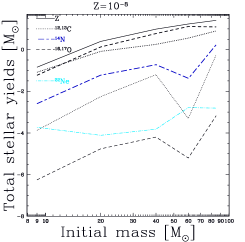
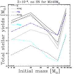
Figure 9: Total stellar yields as a function of the initial mass of the models with $Z=10^{-8}$ and (left) assuming the SN ejects matter for $M\gtrsim 40$ $M_{\odot}$ and (right) assuming direct black hole formation and no matter ejection by the SN for $M\gtrsim 40$ $M_{\odot}$.

In Fig. 9, the two possible outcomes for very massive stars are compared. On the left, the stellar yields include the SN contribution and on the right, the stellar yields only include the wind contribution for stars with $M\gtrsim 40$ $M_{\odot}$. As can be expected, the two outcomes give very different yields for the 40 and 60 $M_{\odot}$ since they do not lose much mass before the SN explosion. For stars above about 60 $M_{\odot}$, the difference is much smaller because the strong winds peal off most of the CNO rich layers before the final collapse.

4.1.1 Metallicity dependence of the CNO yields

The metallicity dependence of the yields can be studied using the 20 $M_{\odot}$ models. Indeed when the yields are convolved by a Salpeter (1955) like initial mass function, 20 $M_{\odot}$ is not far from the average massive star. Note that it is however uncertain whether a standard IMF applies at very low metallicities. Recent studies tend to argue that the IMF is top heavy but very massive stars (VMS, $M\gtrsim 140M_{\odot}$) are not necessary to reproduce observations (see for example Schneider et al., 2006; Tumlinson et al., 2004).

The yields for ¹²C, ¹⁴N and ¹⁶O are presented in Fig. 10.

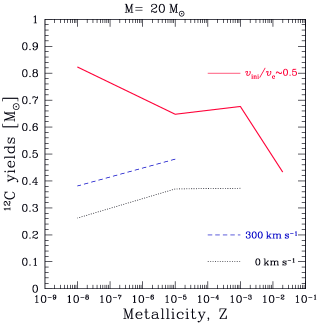
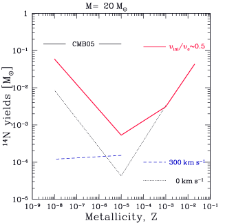
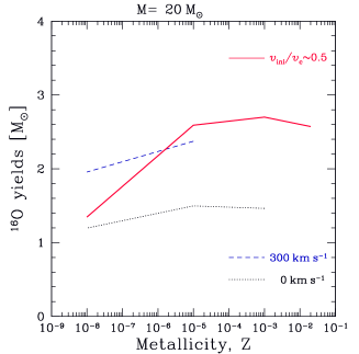
Figure 10: ¹²C (left), ¹⁴N (centre) and ¹⁶O (right) total stellar yields as a function of the initial metallicity of the 20 $M_{\odot}$ models. The red solid curves corresponds to the models with fast rotation, the blue dashed curve to the very low metallicity models with $\upsilon_{\rm ini}$=300 km s^-1 and the dotted black curve to the non–rotating models. In the graph of the ¹⁴N yields, the yields used in the chemical evolution models of Chiappini et al. (2005) in order to reproduce observations is marked with the symbol CMB05. For the fast rotating models, one sees that the carbon yield increases slightly between $Z=10^{-5}$ and $Z=10^{-8}$. At the same time, the oxygen yield decreases towards lower $Z$ by a factor about two.

The most stringent observational constraint at very low Z is a very high primary ¹⁴N production. This requires extremely high primary ¹⁴N production in massive stars, of the order of 0.1 $M_{\odot}$ per star ($\sim$0.15 $M_{\odot}$ used in the heuristic model of Chiappini et al., 2005). In Fig. 10, we can see that only the model at $Z=10^{-8}$ and with a fast rotation ($\upsilon_{\rm ini}=$600 km s^-1) gets close to such high values. The bulk of ¹⁴N is produced in the convective zone created by shell hydrogen burning (see Sect. 3.3). If this convective zone deepens enough to engulf carbon (and oxygen) rich layers, then significant amounts of primary ¹⁴N can be produced (0.01$\sim$0.1$\,M_{\odot}$). This occurs in both the non–rotating model and the fast rotating model but for different reasons. In the non–rotating model, it occurs due to structure rearrangements similar to the third dredge–up at the end of carbon burning (see also Chieffi & Limongi, 2004, for a similar process in Z=0 models). In the model with $\upsilon_{\rm ini}=$600 km s^-1 it occurs during shell helium burning because of the strong mixing of carbon and oxygen into the hydrogen shell burning zone. Another interesting feature is the possible upturn of the [C/O] ratio observed at very low metallicities (ratio between the surface abundances of carbon and oxygen relative to solar; see Fig. 14 Spite et al., 2005). Indeed, the models at $Z=10^{-8}$ with a fast rotation have high C and low O yields compared to the $Z=10^{-5}$ models and could reproduce such an upturn. As explained in Sect. 3.3, the reason is the reduction of the He–burning core mass after the shell H–burning boost induced by strong mixing. As can be seen in Fig. 2, this occurs for all initial masses calculated in the $Z=10^{-8}$ series. The stellar yields of the fast rotating models calculated here were used in a galactic chemical evolution model and successfully reproduce the early evolution of CNO elements (Chiappini et al., 2006). This is a good argument in favour of fast rotation at very low metallicities. Note that in Chiappini et al. (2006), the SN contribution was included in the stellar yields for all masses. The impact of including only the wind contribution for masses above 40 $M_{\odot}$ will be studied in the future. The impact of the important primary nitrogen production and of the other yields on the initial composition and therefore on the evolution of the next stellar generations and their yields is an interesting aspect that will also be studied in the future.

4.1.2 $Z=10^{-8}$ models

The stellar yields of the fast rotating $Z=10^{-8}$ models are presented in Fig. 9. It shows that the significant (above 0.01 $M_{\odot}$) production of primary nitrogen occurs for the entire mass range. For massive stars with $40<M<60\,M_{\odot}$, the yields depend on whether or not the SN contributes to the total yields as discussed earlier. The production of nitrogen is accompanied by a production of ¹³C and ¹⁷O (and to a lesser extent ¹⁸O). The ratio ¹²C/¹³C is very different between the wind and the SN contributions. It is around 5 for the wind and more than 100 for the SN and SN+wind contributions. This, with the N/C and N/O ratios are good tests to differentiate between the two contributions. Part of the primary nitrogen also captures two $\alpha$–particles and becomes ²²Ne. The primary ²²Ne yields are of the order of $10^{-4}\,M_{\odot}$. ²²Ne is one of the main neutron sources for the weak s–process in massive stars. With a low initial iron content due to the low initial overall metallicity, the s–process could occur with a high neutron to seed ratio and produce surprising results. This will be the subject of a future study.

4.2 Carbon rich EMP stars

The zoo of the extremely metal poor stars has been classified by Beers & Christlieb (2005). Carbon rich extremely metal poor stars (CEMPs also called CRUMPs at a recent meeting at Tegernsee, http://www.mpa-garching.mpg.de/$\sim$crumps05) are different from normal EMP star and are rarer (Ryan et al., 2005). About three quarter of the CEMPs show a standard s–process enrichment pointing to the fact that they have accreted matter from an AGB companion in a binary system (Suda et al., 2004). The other CEMP stars show a weak s–process enhancement. Their peculiar abundances are therefore thought to originate from the previous generation of stars. The two most metal poor stars known to date, HE1327-2326 (Frebel et al., 2005; Aoki et al., 2006; Frebel et al., 2006) and HE 0107-5240 (Christlieb et al., 2004; Bessell et al., 2004) are both CEMP stars with a weak s–process enrichment. Chieffi & Limongi (2002) and Nomoto et al. (2005) have studied the enrichment due to PopIII SNe. By using one or a few SNe and using a very large mass cut, they are able to reproduce the abundance of most elements (Limongi et al., 2003; Iwamoto et al., 2005). However they are not able to reproduce the nitrogen surface abundance of HE1327-2326 without rotational mixing or the oxygen surface abundance of HE 0107-5240 without mixing and fall–back mimicking an aspherical explosion. In this work, the impact of rotation is explored. HE1327-2326 is characterised by very high N, C and O abundances, high Na, Mg and Al abundances, a weak s–process enrichment and depleted lithium. The star is not evolved so has not had time to bring self–produced CNO elements to its surface and is most likely a subgiant (Korn, presentation at the CRUMPS meeting). A lot of the features of this star are similar to the properties of the stellar winds of very metal poor rotating stars (Meynet et al., 2006).

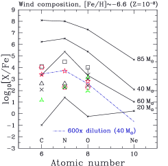
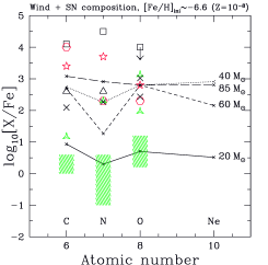
Figure 11: Composition in [X/Fe] of the stellar wind (left) and the mixture of the wind and SN ejecta (right) for the $Z=10^{-8}$ models. The lines represent predictions from the models. The following symbols correspond to the values obtained from measurements at the surface of giant CEMP stars: red hexagons for HE 0107-5240, [Fe/H]$\simeq$ -5.3 (Christlieb et al., 2004); green thin triangles CS 22949-037, [Fe/H]$\simeq$ -4.0 (Norris et al., 2002; Depagne et al., 2002; Israelian et al., 2004b); crosses CS 29498-043, [Fe/H]$\simeq$ -3.5 (Aoki et al., 2004). Two values are given for oxygen for the last two stars. They come from the determinations using O triplet or [OI] forbidden lines (Aoki et al., 2004; Israelian et al., 2004b). The empty triangles (Plez & Cohen, 2005), [Fe/H]$\simeq-4.0$ and squares (Frebel et al., 2005), [Fe/H]$\simeq-5.4$ correspond to non-evolved CEMP stars. The new (3D/NLTE corrected) estimates for HE1327-2326 from Frebel et al. (2006) are represented by the red stars. On the right, wind+SN ejecta are compared to the normal EMP stars (green hatched area with lines going down to the right Cayrel et al., 2004; Spite et al., 2005) for the 20 $M_{\odot}$ model and again to the CEMP stars for the more massive models. For this purpose, the value [O/Fe] is chosen to fall in the middle of the observed range (20 $M_{\odot}$: [O/Fe]=0.7 and $M>20\,M_{\odot}$: [O/Fe]=2.8). For HE1327-2326, the best fit for the CNO elements is obtained by diluting the composition of the wind of the 40 $M_{\odot}$ model by a factor 600.

HE1327-2326 could therefore have formed from gas, which was mainly enriched by stellar winds of rotating very low metallicity stars. In this scenario, a first generation of stars (PopIII) pollutes the interstellar medium to very low metallicities ([Fe/H]$\sim$-6). Then a PopII.5 star (Bromm, 2005; Hirschi, 2005; Karlsson, 2006) like the 40 $M_{\odot}$ model calculated here pollutes (mainly through its wind) the interstellar medium out of which HE1327-2326 forms. This would mean that HE1327-2326 is a third generation star. In this scenario, the CNO abundances are well reproduced, in particular that of nitrogen, which according the new values for a subgiant from Frebel et al. (2006) is 0.9 dex higher in [X/Fe] than oxygen. This is shown in Fig. 11 where the new abundances are represented by the red stars and the best fit is obtained by diluting the composition of the wind of the 40 $M_{\odot}$ model by a factor 600. On the right side of Fig. 11, one sees that when the SN contribution is added, the [X/Fe] ratio is usually lower for nitrogen than for oxygen. The lithium depletion cannot be explained by rotational and convective mixing in the massive star if the wind material is diluted in the ISM by a factor 600 (600 parts of ISM for 1 part of wind material) as is suggested above. However, if the wind material is less enriched in CNO elements, a lower dilution factor would be necessary to reproduce the observations. Also if the massive star is born with a higher iron content, a lower dilution factor is necessary. If this dilution factor is of the order of unity, it becomes possible to explain the lithium depletion by internal mixing in the massive star. To investigate this possibility, more models have to be calculated with different initial metallicities. Although the existence of a lower limit for the minimum metallicity $Z$ for low mass stars to form is still under debate, It is interesting to note that the very high CNO yields of the 40 $M_{\odot}$ stars brings the total metallicity $Z$ above the limit for low mass star formation obtained in Bromm & Loeb (2003).

For HE 0107-5240 (red hexagons in Fig. 11), rotation does not help since neither the wind contribution nor the total contribution produce such large overproduction of carbon compared to nitrogen and oxygen. Possible origins for this star are presented in Iwamoto et al. (2005) and (Suda et al., 2004). For the other carbon rich stars presented in Fig. 11, the oxygen abundances are either not determined or still quite uncertain (Izotov & Thuan, 2004). The C and N surface abundances of G77-61 (Plez & Cohen, 2005) could originate from material similar to the wind of the 85 $M_{\odot}$. The C and N surface abundances of CS 22949-037 (Norris et al., 2002; Depagne et al., 2002; Israelian et al., 2004b) resemble the wind composition of the 60 $M_{\odot}$ model although some oxygen needs be ejected from the supernova. The enrichments in C, N and O are very similar for CS 29498-043 (around +2, see Aoki et al., 2004) and a partial ejection due to the supernova is necessary to explain the oxygen enrichment since in the winds the oxygen is usually under produced compared to C and N. It will be interesting to follow the evolution of Na, Mg and Al since the high yields of ²²Ne seem to indicate that there could an overproduction of these elements in the wind (see Table 3 and the $Z=10^{-5}$ model presented in Meynet et al., 2006). Since ²²Ne is also a neutron source, s–process calculations are also planned.

5 Conclusion

Two series of models were computed. The first series consists of 20 $M_{\odot}$ models with varying initial metallicity (solar down to $Z=10^{-8}$) and rotation ($\rm\upsilon_{ini}=0-600$ km s^-1). The second one consists of models with an initial metallicity of $Z=10^{-8}$, masses between 9 and 85 $M_{\odot}$ and fast initial rotation velocities. The results presented confirm the crucial role of rotation in stellar evolution and its impact in very low metallicity stars (Meynet et al., 2006). The evolution of the models with $Z=10^{-8}$ ([Fe/H]$\sim-6.6$) is very interesting. In the course of helium burning, carbon and oxygen are mixed into the hydrogen burning shell. This boosts the importance of the shell and causes a reduction of the CO core mass. Later in the evolution, the hydrogen shell deepens and produces large amount of primary nitrogen. For the most massive models ($M\gtrsim 60$ $M_{\odot}$), significant mass loss occurs during the red supergiant stage assuming that CNO elements are important contributors to mass loss. This mass loss is due to the surface enrichment in CNO elements via rotational and convective mixing. The models predict the production of WR stars for an initial mass higher than 60 $M_{\odot}$ at $Z=10^{-8}$ and the 85 $M_{\odot}$ model becomes a WO. Therefore SNe of type Ib and Ic are predicted from single massive stars at these low metallicities. The 85 $M_{\odot}$ model retains enough angular momentum to produce a GRB but the calculations did not include the effects of magnetic fields.

The stellar yields are presented for light elements. These yields were used in a galactic chemical evolution model and successfully reproduce the early evolution of CNO elements (Chiappini et al., 2006). A scenario is also proposed to explain the abundances of the most metal poor star known to date HE1327-2326 (Frebel et al., 2005). In this scenario, a first generation of stars (PopIII) pollutes the interstellar medium to very low metallicities ([Fe/H]$\sim$-6). Then a PopII.5 star (Bromm, 2005) like the 40 $M_{\odot}$ model calculated in this study pollutes only with its wind the interstellar medium out of which HE1327-2326 forms.

There are still many questions or issues that could not be treated in this work. It is necessary to determine over which metallicity range the large primary production and the other specific features of the $Z=10^{-8}$ models occur. The impact of the yields on the initial composition and therefore on the evolution of the next stellar generations also needs to be studied. It will also be interesting to follow the evolution of Na, Mg and Al since the high yields of ²²Ne seem to indicate that there could an overproduction of these elements in the wind (see Table 3 and the $Z=10^{-5}$ model presented in Meynet et al., 2006). Since ²²Ne is also a neutron source, s–process calculations are also planned. The effects of magnetic fields (Yoon & Langer, 2005; Woosley & Heger, 2006; Maeder & Meynet, 2005) on the results will be studied in the near future. The dependence of the mass loss rates on the metallicity, especially in the RSG stage need to be further studied to see how the results of van Loon (2005, mass loss in the RSG phase independent of metallicity) can be extrapolated to very low metallicities.