The Optimum Distance at which to Determine the Size of a Giant Air Shower

Abstract

To determine the size of an extensive air shower it is not necessary to have knowledge of the function that describes the fall-off of signal size from the shower core (the lateral distribution function). In this paper an analysis with a simple Monte Carlo model is used to show that an optimum ground parameter can be identified for each individual shower. At this optimal core distance, $r_{\mathrm{opt}}$, the fluctuations in the expected signal, $S(r_{\mathrm{opt}})$, due to a lack of knowledge of the lateral distribution function are minimised. Furthermore it is shown that the optimum ground parameter is determined primarily by the array geometry, with little dependence on the energy or zenith angle of the shower or choice of lateral distribution function. For an array such as the Pierre Auger Southern Observatory, with detectors separated by 1500 m in a triangular configuration, the optimum distance at which to measure this characteristic signal is close to 1000 m.

1 Introduction

The extreme rarity of the largest extensive air showers necessitates an observatory of large aperture if large numbers of events are to be recorded. In the case of an array of surface detectors, the need to cover as large an area as possible, combined with inevitable economical constraints, invariably leads to an array with large separation between adjacent detectors. The result is that properties of any individual air shower are sampled at a limited number of points at different distances from the shower core. When reconstructing the size of the shower, the lateral distribution function (LDF), which describes the fall-off of signal size with the distance from the shower core, must be assumed and any inaccuracies in it (either from uncertainties in the form of the LDF or from intrinsic fluctuations in the development of the air shower) will lead to a corresponding inaccuracy in both the location of the shower core and in the measurement of the integrated LDF (traditionally a measure of the total number of particles in the shower). To avoid the large fluctuations in the signal integrated over all distances, Hillas hillas , hillas1 proposed using the signal at some distance from the shower core to classify the size of the shower, and ultimately the energy of the primary particle. In his original paper he pointed out the practical advantages of this method: (i) the effect of uncertainties in the LDF are minimised at a particular core distance, and (ii) although the total number of particles at ground level is subject to large fluctuations, the fluctuations of the particle density far from the core are quite small. For example in ref.hillas it is shown that at $10^{17}$ eV the RMS variation in the total number of particles is $\approx 67$ %; for the same shower the RMS variation in the signal of a water-Cherenkov detector at 950 m is $\approx 6$ %. While these absolute numbers are certainly model dependent, his conclusion was shown to be robust for a variety of models and energies.

The measurement of the energy of a primary particle with a surface array of particle detectors, is thus a two-step process. Firstly the detector signal at a particular core distance must be measured and secondly this characteristic signal must be linked to the energy of the primary particle. The choice of the distance at which to measure this characteristic signal will depend on the combined (and independent) uncertainties of each step. All cosmic ray observatories which employ surface detectors (with the notable exception of the Pierre Auger Observatory) have relied on models to perform the second step. Systematic uncertainties aside, the effects of intrinsic shower-to-shower fluctuations are minimised if the characteristic signal (the shower ground parameter) is measured at a core distance of $\gtrsim 600$ m hillas , hillas1 . The Pierre Auger Observatory eapaper , with the benefit of its hybrid design, utilises fluorescence detectors to measure around 10% of the EASs observed with the surface array. The calorimetric energy measurement from the fluorescence detectors can be used to calibrate the characteristic signal from the surface detectors sommers , thus substantially reducing a large source of systematic uncertainty.

The optimum core distance for the first step, the measurement of a characteristic signal, is solely dependent on the geometry of the array. The optimum distance to measure the shower ground parameter, S($r_{\mathrm{opt}}$), can be identified for each individual event. The work of Hillas led to the Haverah Park Collaboration adopting $\rho(600)$, the particle density at 600 m from the shower core measured in a 1.2 m deep water-Cherenkov detector, as the optimum energy estimator.

Identifying this optimum core distance, $r_{\mathrm{opt}}$, is especially relevant to giant arrays, where the large array spacing (typically $\gtrsim 1$ km) makes measuring the LDF problematic, except in events of very high multiplicity. The low number of signals obtained from any one event usually makes measurement of the LDF on an event-by-event basis impractical. Instead an average LDF, parameterised in measurable observables such as zenith angle and energy, must be used. Even if the average LDF can be measured to a high degree of accuracy (which may not always be possible with a surface detector alone), intrinsic shower-to-shower fluctuations will affect the lateral structure of any particular event, often characterised as the slope of the LDF, describing how rapidly the particle density decreases with core distance. Identifying the optimum core distance at which to measure the characteristic signal of an air shower, will minimise the uncertainty in this parameter due to a lack of knowledge of the true LDF.

In this paper, a method of identifying this optimum ‘ground parameter’, where the observed signal shows the least dependence on the assumed LDF, is discussed and its dependence on energy, zenith angle and array geometry is investigated.

2 Simple Monte Carlo Analysis

The signals observed by an array of surface detectors were simulated using a simple Monte Carlo technique. This was achieved by adopting a lateral distribution function for an extensive air shower:

$$S(r)=k\,f(\beta,r)\,,$$

where $S(r)$ is the signal observed at a core distance $r$, $k$ is a size parameter, and $f(\beta,r)$ is the functional form of the LDF, parameterised as a function of the slope parameter, $\beta$, and the core distance, $r$. Throughout this paper, the signal is expressed as that relative to a vertical equivalent muon (VEM), although any arbitrary unit would give a similar result. The simulated shower was projected onto a virtual array with a specified core location and arrival direction and the signals in each tank, at the calculated core distance, were given by the assumed LDF. The signals were then varied according to a Poissonian distribution in the number of particles, assuming each particle contributes 1 VEM. Signals below a threshold of 3.2 VEM were set to zero, and those above 1000 VEM were treated as saturated. These values were chosen to accord with what is currently used at the Auger Observatory. Using the known arrival direction as an input, the event can then be analysed to assess the reconstruction algorithm, in particular the effect of using an incorrect LDF.

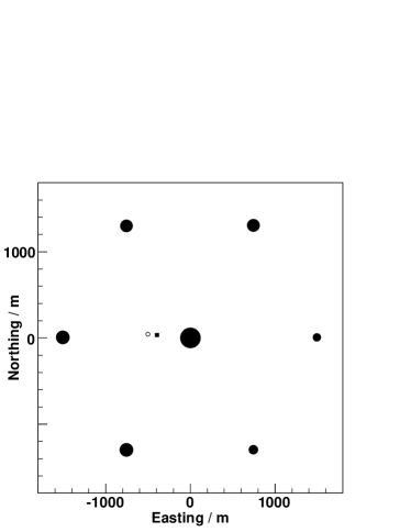
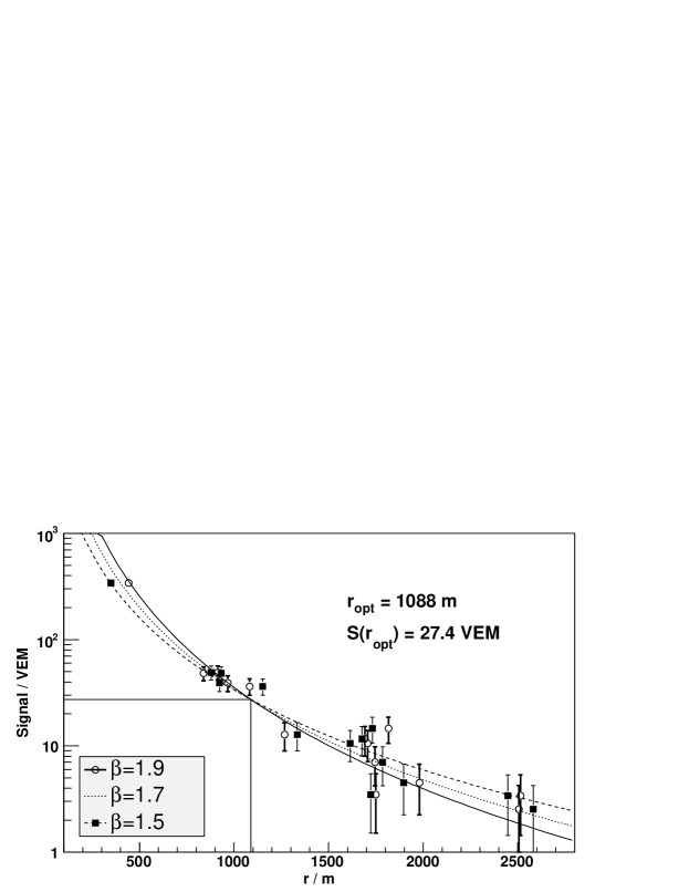
Figure 1: The optimum core distance for one event. The same event was reconstructed with an ‘NKG’ type LDF, using two different values for the slope parameter: $\beta=1.5$ (filled squares), $\beta=1.7$ (dotted line), and $\beta=1.9$ (circles). The different slope parameters result in different reconstructed core locations (separated by $\sim 100$ m), indicated by the open circle and the square on the plan of part of the array (top) where the black points indicate tanks with a signal and the size of the point is proportional to the logarithm of the signal. Both reconstructions give reasonable fits to the signals (bottom). The dotted line shows the reconstruction using an intermediate value of $\beta=1.7$ (points not plotted). At $\sim r_{\mathrm{opt}}$, the same signal ($\sim 27$ VEM) is measured for each reconstruction, and by converting this ground parameter, $S(r_{\mathrm{opt}})$ into the energy of the primary particle, uncertainties due to a lack of knowledge of the true slope parameter are minimised.

A hexagonal array was chosen with detector spacing of 1500 m corresponding to that of the Pierre Auger Southern Array. The dependence of the event reconstruction on the slope parameter of the LDF is shown in figure 1. For this single event the input LDF was an ‘NKG’ type function with the form

$$S=k\left(\frac{r}{r_{s}}\right)^{-\beta}\left(1+\frac{r}{r_{s}}\right)^{-\beta}\,.$$

The slope parameter $\beta$ was parameterised as a function of zenith angle, $\theta$, such that $\beta=2.5-(\sec\theta-1)$ , the scaling parameter, $r_{s}$ was set to 700 m and the size parameter, $k$, was set to 250 (comparisons with full Monte Carlo simulations suggest this corresponds to a shower initiated by a primary with energy of $\sim 10$ EeV). The zenith angle was set to $55^{\circ}$. From this LDF signals for each tank were drawn and varied according to typical (Poissonian) measurement uncertainties, as described above. To reconstruct the shower, the ‘NKG’ type function was used to fit the location of the shower core and the size parameter, $k$, simultaneously. The reconstruction of the event was carried out three times using different fixed values for the slope parameter $\beta$ with each reconstruction. The effect of the differing values for the slope of the LDF is clearly seen in figure 1. While the fits result in a substantial shift in the reconstructed core location (of $\sim 100$ m) and corresponding shifts in the core distances of the individual detectors, it is evident that the characteristic signal for this event, at $\sim 1090$ m, is very similar for all three reconstructions. Measuring the signal at this point minimises the effect of the systematic uncertainty in the slope parameter of the LDF.

3 Determining $r_{\mathrm{opt}}$

To find the distance, $r_{\mathrm{opt}}$, for which the signal variation with respect to the slope parameter, $\beta$, is smallest, one can minimise $\frac{dS}{d\beta}$. For a power law LDF, this is shown in the following.

$$S=kr^{-\beta}=ke^{-\beta\ln r}\ ,$$

where $S$ is the predicted signal, k is the shower size parameter and $\beta$ is the slope parameter.

If $k=k(\beta)$,

$$\frac{\mathrm{d}S}{\mathrm{d}\beta}=\frac{\mathrm{d}k}{\mathrm{d}\beta}e^{-\beta\ln r}+ke^{-\beta\ln r}(-\ln r)$$ (1)

$\frac{\mathrm{d}S}{\mathrm{d}\beta}=e^{-\beta\ln r}\left(\frac{\mathrm{d}k}{\mathrm{d}\beta}-k\ln r\right)=0$, at $r_{\mathrm{opt}}$

so,

$$\frac{\mathrm{d}k}{\mathrm{d}\beta}=k\ln r_{\mathrm{opt}}$$

and,

$$\frac{\mathrm{d}\ln k}{\mathrm{d}\beta}=\ln r_{\mathrm{opt}}$$ (2)

A similar deduction can be applied to different classes of LDF, such as a ‘Haverah Park’ function:

$$S=kr^{-(\beta+\frac{r}{4000})}$$

$$\Rightarrow\frac{\mathrm{d}(\ln k)}{\mathrm{d}\beta}=\ln r_{\mathrm{opt}}\,,$$

or an ‘NKG’ type function:

$$S=k\left(\frac{r}{r_{s}}\right)^{-\beta}\left(1+\frac{r}{r_{s}}\right)^{-\beta}$$

$$\Rightarrow\frac{\mathrm{d}(\ln k)}{\mathrm{d}\beta}=\ln\left(\frac{r_{\mathrm{opt}}}{r_{s}}\right)+\ln\left(1+\frac{r_{\mathrm{opt}}}{r_{s}}\right)$$ (3)

which leaves a quadratic equation to be solved to find $r_{\mathrm{opt}}$:

$$\frac{r_{\mathrm{opt}}}{r_{s}}=\frac{-1+\sqrt{1+4e^{\alpha}}}{2}$$ (4)

where $\alpha=\frac{\mathrm{d}(\ln k)}{\mathrm{d}\beta}$.

Of course, in a real event, the observed signals are subject to a measurement uncertainty and the LDF must be fitted to the data using a suitable minimisation procedure, but using reasonable values for $\beta$ and the size of the fluctuations gives a good approximation to this analytical solution. $r_{\mathrm{opt}}$ can then be found for any event by analysing it several times, using different values for the slope parameter and either plotting $ln\,k$ against $\beta$, or numerically minimising the spread of S(r) at any core distance, $\Delta S(r)$.

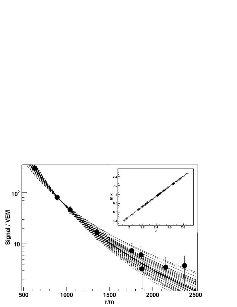
Figure 2: Reconstructing the same event 50 times, using different values for the slope parameter, $\beta$, allows the optimum ground parameter, $r_{\mathrm{opt}}$ to be found (using an ‘NKG’ type LDF in this example). At $r_{\mathrm{opt}}$, the expected signal is essentially independent of the slope parameter. The inset plot shows the relationship between the slope parameter and the fitted size parameter, allowing $r_{\mathrm{opt}}$ to be calculated analytically (equation 3).

A simulated event is shown in figure 2 after reconstructing the event 50 times, using values of the slope parameter, $\beta$, drawn from a Gaussian distribution with a mean of 2.4 and a width of 10%, which corresponds approximately to the uncertainty in $\beta$. The zenith angle of the event is $24^{\circ}$ and the size parameter, $k$, was set to 1050 (again, corresponding to a primary energy of $\sim 10$ EeV). The value taken for the magnitude of the intrinsic fluctuations in the slope parameter is based on measurements made at Haverah Park ave , coy , which indicate that 10% is an appropriate value. Fluctuations of a similar magnitude were measured at Volcano Ranch vr . The reconstructed LDFs can be seen to converge at around 940 m. The inset panel shows $\beta\,vs\,\ln k$ found from the 50 reconstructions. The relationship is approximately linear and, using the formula given in equation 3, the spread in $S(r)$ is found to be minimised at 938 m. The spread, $\Delta S(r)$, at any core distance corresponds to the systematic uncertainty in $S(r)$ due to the uncertainty in the slope parameter, $\beta$ and can be found analytically by equating

$$\frac{dS(r)}{d\beta}\approx\frac{\Delta S(r)_{\mathrm{sys}}}{\Delta\beta}$$

and rearranging equation 1 for the appropriate LDF.

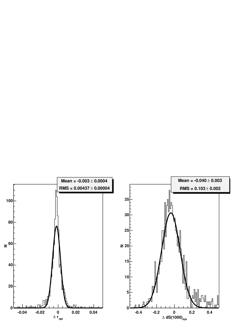
Figure 3: Comparing the optimum ground parameter (left) and the systematic uncertainty in S(1000) (right) found using a numerical and an analytical technique. In each case the residual is shown as $\frac{numerical-analytical}{numerical}$. The statistics refer to the Gaussian fit.

A comparison of the analytical and numerical techniques, found from 1000 simulated showers is shown in figure 3. Each shower had a randomly assigned zenith angle, $\theta$, of between 0 and $60^{\circ}$ following a flat distribution in $\sec\theta$. The size parameter, $k$, was also randomly assigned from a flat distribution, to give a range of equivalent energies of between 5 and 100 EeV. The slope parameter, $\beta$ for each event had the mean value found using the parameterisation given in section 2, but was then varied according to a Gaussian distribution with a width of 10 %. The resulting values of $r_{\mathrm{opt}}$ and $\Delta S(1000)_{\mathrm{sys}}$ agree within 1% and 10 % respectively, demonstrating that the analytical technique is a good approximation to the numerical analysis.

3.1 Saturated Signals

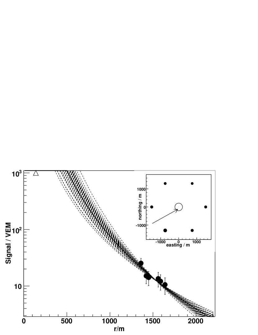
Figure 4: $r_{\mathrm{opt}}$ for a saturated, vertical ($\theta=24^{\circ}$) event. With 6 tanks at roughly the same distance ($\sim 1500$ m), this is the optimum point to measure the shower ground parameter. The open triangular point indicates the saturated tank. The inset plot shows a plan of the array - the saturated tank (open circle) is surrounded by a hexagon of tanks with signals (filled circles). The shower core and azimuthal direction are indicated by the arrow .

If, by chance, a shower core lies close to one tank, the signal in that tank may be saturated: for the Auger Observatory, currently, saturation occurs for signals larger than $\approx$ 1000 VEM. The effect of a saturated signal on the reconstruction algorithm can be seen in figure 4. This vertical shower has one saturated tank, then a ring of 6 tanks with similar signals, all lying at about 1500 m from the core. The reconstructed values are only weakly constrained by the presence of the saturated tank, and so $r_{\mathrm{opt}}$ is found at the point where most of the signals are measured ($\sim 1500$ m).

3.2 Dependence on Zenith Angle and Energy

An analysis of 1000 showers with zenith angles between 0 and $60^{\circ}$ and size parameters such that $5<E<100$ EeV gives the distribution of $r_{\mathrm{opt}}$ shown in figure 5 (top left panel). The distribution has two distinct populations corresponding to events with and without saturated signals. The mean value for the showers without a saturated signal is $970\pm 1$ m and the RMS deviation is $102\pm 1$ m. The mean spread in $S(r)$ as a function of $r$ is shown in the upper right panel of the same figure. If the characteristic signal size is measured at 970 m for all the showers, the mean systematic uncertainty in this measurement is less than 2%, although this increases to $\sim 10$ % for the events with a saturated signal. The relatively small change of $r_{\mathrm{opt}}$ with zenith angle is clear in the bottom left hand diagram of the figure.

If the same events are reconstructed with different forms of LDF, such as a power law or a ‘Haverah Park’ type LDF, the optimum ground parameters can be found with the same technique and give similar results as those found using the ‘NKG’ type function. The distribution of $r_{\mathrm{opt}}$, for the events without a saturated signal, found using 3 different LDFs are shown in table 1. Also shown in table 1 are the values of S(1000) measured with each LDF, normalised to S(1000) measured with the ‘NKG’ type LDF. The agreement between the values of S(1000) found using these 3 different LDFs is better than 5%.

LDF	$r_{\mathrm{opt}}$ / m, mean	$r_{\mathrm{opt}}$ / m, RMS	$\Delta S(1000)=\frac{S(1000)_{\mathrm{LDF}}}{S(1000)_{\mathrm{NKG}}}$
Power Law	960	110	$1.045\pm 0.001$
‘Haverah Park’	940	100	$0.986\pm 0.001$
‘NKG’ type	970	110	1.00

Table 1: The optimum ground parameter found using 3 different LDFs

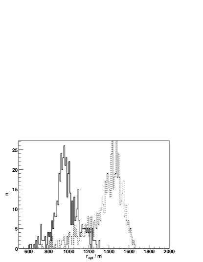
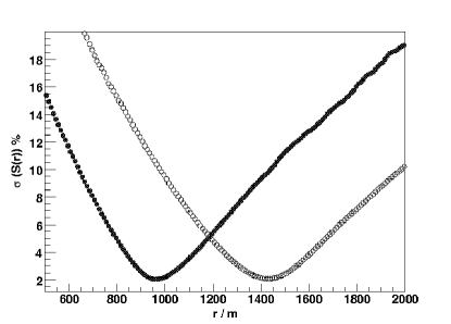
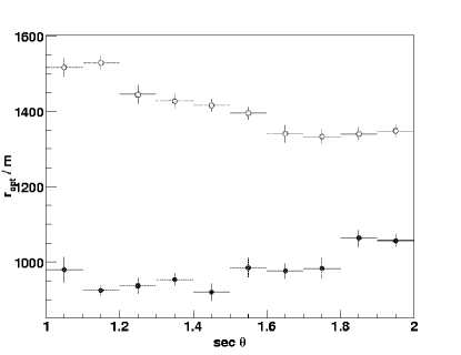
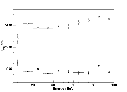
Figure 5: Top left panel: The distribution of $r_{\mathrm{opt}}$ (assuming $10\%$ fluctuations in the slope parameter), for $10$ simulated showers, with zenith angle $1.0<\sec\theta<2.0$ and energies between 5 and 100 EeV. The dashed line shows the distribution of saturated signal while the solid line is for events without a saturated signal. Top right panel: The mean percentage spread in $S(r)$. Bottom row: The dependence of $r_{\mathrm{opt}}$ on the zenith angle, $\theta$, and energy of the primary particle. In all plots, the solid markers indicate events in which there are no saturated signals while the open markers are for events with one or more saturated signals.

The variation of $r_{\mathrm{opt}}$ as a function of the array spacing is shown in figure 6. The relationship is approximately linear with the value of $r_{\mathrm{opt}}$ increasing at a rate of $\sim 45$ m for each 100 m increase in the detector separation.

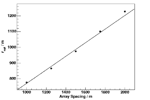
Figure 6: $r_{\mathrm{opt}}$ as a function of the surface array spacing. The uncertainties in $r_{\mathrm{opt}}$ are smaller than the points.

4 Conclusion

An analysis of the events simulated with a simple Monte Carlo model has shown that the optimum core distance to measure the size of the shower can be calculated for each shower and is determined primarily by the array geometry, with no significant dependence on the shower zenith angle, energy or the assumed lateral distribution function (figure 5, table 1). The presence of saturated tanks has a significant impact on $r_{\mathrm{opt}}$, resulting in an increase of up to 500 m (depending on the zenith angle). This will primarily affect large, vertical showers that have a relatively small number of tanks with signals and a high probability of saturation in one tank. The determination of $r_{\mathrm{opt}}$ for these events will depend on the treatment of these signals in the reconstruction algorithm.

For an array with 1500 m spacing, such as the Pierre Auger Observatory, the plot shown in figure 6 indicates that $r=1000$ m is a good choice at which to measure the characteristic signal, S(1000), used to determine the energy of the primary particle. At around 1000 m the expected signal is robust against inaccuracies in the assumed LDF at better than 5%.

5 Acknowledgments

Research on Ultra High Energy Cosmic Rays at the University of Leeds is supported by PPARC, UK. DN is grateful for the support of a PPARC Research Studentship.

References

- [1] Hillas A.M., Acta Phys. Acad. Sci. Hung., 29 (1970), Suppl. 3, 355
- [2] Hillas A. M., Proceedings of the 12th International Conference on Cosmic Rays, vol. 3, 1001, 1971
- [3] Abraham J. et al. (The Pierre Auger Collaboration), NIMA, 523 (2004), 50-95
- [4] Sommers P., for the Pierre Auger Collaboration, Proceedings of the 29th International Cosmic Ray Conference, vol. 7, 387, 2005
- [5] Ave M. et al, Astroparticle Physics, vol. 19 (2003), 61-75
- [6] Coy R.N. et al, Proceedings of the 17th International Conference on Cosmic Rays, vol. 6, 1981
- [7] Linsley J, Proceedings of the 15th International Conference on Cosmic Rays, vol. 12, pp (56, 62, 89), 1977