The Advantage of Increased Resolution in the Study of Quasar Absorption Systems

Abstract

We compare a new $R=120,000$ spectrum of PG $1634+706$ ($z_{QSO}=1.337,m_{V}=14.9$) obtained with the HDS instrument on Subaru to a $R=45,000$ spectrum obtained previously with HIRES/Keck. In the strong Mgii system at $z=0.9902$ and the multiple cloud, weak Mgii system at $z=1.0414$, we find that at the higher resolution, additional components are resolved in a blended profile. We find that two single-cloud weak Mgii absorbers were already resolved at $R=45,000$, to have $b=2$-$4$ km s^-1. The narrowest line that we measure in the $R=120,000$ spectrum is a component of the Galactic Nai absorption, with $b=0.90\pm 0.20$ km s^-1. We discuss expectations of similarly narrow lines in various applications, including studies of DLAs, the Mgi phases of strong Mgii absorbers, and high velocity clouds. By applying Voigt profile fitting to synthetic lines, we compare the consistency with which line profile parameters can be accurately recovered at $R=45,000$ and $R=120,000$. We estimate the improvement gained from superhigh resolution in resolving narrowly separated velocity components in absorption profiles. We also explore the influence of isotope line shifts and hyperfine splitting in measurements of line profile parameters, and the spectral resolution needed to identify these effects. Super high resolution spectra of quasars, which will be routinely possible with 20-meter class telescopes, will lead to greater sensitivity for absorption line surveys, and to determination of more accurate physical conditions for cold phases of gas in various environments.

1 INTRODUCTION

With the advent of high resolution spectroscopy on 8-meter class telescopes in the early 1990’s came a revelation in the study of quasar absorption line systems. Previous to this time, several large surveys were conducted with a typical resolution of $R=\lambda/\Delta\lambda=1000$–$3000$, corresponding to $100$–$300$ km s^-1. These surveys tabulated the redshift path densities of Mgii, Civ, and Ly$\alpha$ lines over the redshift range accessible from optical telescopes (Lanzetta et al., 1987; Sargent et al., 1988; Caulet, 1989). However, most individual systems were not resolved, so that the kinematics of the different metal lines could not be compared system by system. It is not surprising that an increase of resolution to $R=45,000$ ($\sim 7$ km s^-1) provided detailed views of the multiphase structure of gas inside and around galaxies, since parcels of gas within the different components of galaxies are often moving at several to tens of km s^-1 relative to one another. The increase of resolution from thousands to tens of thousands also brought a dramatic increase in the sensitivity of surveys. This allowed measurements of the metallicity in the most diffuse gas sampled by weak Ly$\alpha$ forest lines (e.g., Cowie et al., 1995), and for deeper surveys of metal lines as well (e.g., Churchill et al., 1999; Misawa et al., 2002).

Presently, hundreds of quasar spectra have been obtained with $R\sim 45,000$ using the High Resolution Echelle Spectrograph on Keck I (HIRES, Vogt et al., 1994), the High Dispersion Spectrograph on Subaru (HDS, Noguchi et al., 1999) and the Ultraviolet-Visual Echelle Spectrograph on the VLT (UVES, Dekker et al., 2000). There is undoubtedly much to be gained from detailed studies of the absorption lines detected in these databases. However, in this paper we look toward the future and ask what advances we should expect in studies of quasar absorption lines with an increase in resolution from the presently attainable value of $7$ km s^-1 to $0.5$-$2$ km s^-1, which is within the reach of 20-meter class telescopes for hundreds of quasars. This follows a study by Tappe & Black (2004) of the quasar PKS $2145+067$ at $R\sim 100,000$ with UVES on the VLT UT2 telescope. That study focused on the $z=0.79089$ strong Mgii absorber, and measured $b$ parameters in the range $1$–$7$ km s^-1, showing considerably more structure than previous spectra (Churchill et al., 2001) with $R\sim 45,000$. More recently, Chand et al. (2006) considered the effect of observing at $R>100,000$ for studies of variation in the fine-structure constant.

In addition to the increased sensitivity to weak lines, gained at higher resolution, there is reason to expect we should see substructure on km s^-1 scales. Distinct small-scale structures are seen in the interstellar medium of the Milky Way on these velocity scales (Points et al., 2004). Very narrow components, indicating cold clouds, are seen through 21-cm absorption in some damped Ly$\alpha$ systems (Lane et al., 2000). Also, detailed models of transitions detected in DLA systems indicate the presence of a cold phase (Wolfe et al., 2003). The large Mg to Mg⁺ ratios in many components of strong Mgii absorbers, most of which are produced by lines of sight through $L^{*}$ galaxies, could be explained by a cold phase that produces the bulk of the Mgi absorption (Churchill et al., 2003). In the case of the $z=0.9902$ system toward PG$1634+706$, Ding et al. (2003) proposed cold clouds with Doppler parameters of $b(Mg)\sim 0.75$ km s^-1 to explain the strong Mgi absorption, but these could not be resolved at FWHM$\sim 7$ km s^-1. Finally, VLA observations of Milky Way high velocity clouds indicate that they have $T<900$ K, and most Milky Way lines of sight show narrow Caii lines from HVCs (Richter et al., 2005). However, at FWHM$\sim 7$ km s^-1 these Caii lines were unresolved. Richter et al. (2005) suggested that if the Milky Way is typical of spiral galaxy halos these narrow absorption features should be commonly seen in the profiles of strong Mgii absorbers and Lyman limit systems.

For the brightest quasars it is already feasible to use the highest resolution settings on 8-meter class telescopes ($\sim$ 40 with $m_{V}<16$ for non-exorbitant exposure times) to study quasar absorption line systems. In this paper, we present an exploration of the power of $R=120,000$ in studying four Mgii absorbers along the line of sight toward the magnitude $m_{V}=14.9$ quasar PG$1634+706$. Our observations were carried out in the service mode with the HDS on the Subaru Telescope.

The paper begins, in § 2, with a general consideration of how accurately line parameters can be determined at super-high resolution. In § 3, we present our Subaru/HDS observations of several absorption line systems in the spectrum of one of the brightest quasars, PG $1634+706$, and discuss the implications of our $R=120,000$ observations of these systems. We also show the Milky Way absorption along this line of sight. In § 4, we speculate about the progress that will be made in the study of quasar absorption lines when many quasars are observed at $R>100,000$.

2 SIMULATION OF VERY NARROW ABSORPTION LINES

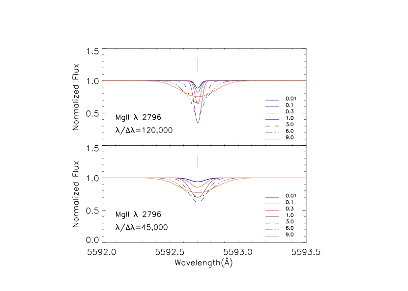
Figure 1: Synthetic absorption profiles of varying Doppler parameter $b$ convolved to spectral resolutions of $R=120,000$ and $R=45,000$. The absorption line is redshifted to $z=1$. The tick marks the center of the absorption profile.

In gas with temperatures T $<8000$ K, most metals would produce absorption features that are narrower than $b_{therm}$ = 2 km s^-1. Figure 1 illustrates progressively narrow absorption profiles of Mgii$\lambda$ 2796 line with column density $N({\hbox{{\rm Mg}${}^{+}$}})=10^{12}$ cm^-2 and with Doppler parameters $b({\hbox{{\rm Mg}${}^{+}$}})$ from $9$ km s^-1 to $0.01$ km s^-1 at high ($R=45,000$) and super-high spectral resolutions ($R=120,000$). The various profiles were produced by convolving a model absorption feature with Gaussian kernels of FWHM = $6.6$ km s^-1 and FWHM = $2.5$ km s^-1, to simulate the resolving powers corresponding to the two spectral resolutions. Comparing the profile shapes, it is apparent that, even at high resolution, the width of intrinsically very narrow lines is often misrepresented. A measurement of the $b$ would result in a value significantly higher than the true value, which further affects the estimation of the upper limit for the gas temperature. To explore the effect of resolution further, we evaluate the consistency with which Voigt profile parameters (i.e., column density and Doppler parameter) can be recovered from very narrow absorption profiles at two resolutions; $R=120,000$ and $R=45,000$ in synthetically simulated spectra. Both these parameters are important for deriving ionization structure, gas phase metallicities, and other physical conditions for the absorber. In addition, using this approach, we also consider two other effects: (1) blending of lines, and (2) isotope shifts and hyperfine splitting in absorption lines. We evaluate the advantage of increased resolution in recognizing these effects and also in determining how they influence Doppler parameter measurements of absorption profiles.

2.1 Very Narrow Single Component Lines

For our simulations we synthesized Mgii $\lambda$ 2796 lines with two sets of values: (1) column density of $N({\hbox{{\rm Mg}${}^{+}$}})$ = $10^{12}$ cm^-2 and $b({\hbox{{\rm Mg}${}^{+}$}})$ = $2.0$ km s^-1, corresponding to a rest-frame equivalent width limit of $W_{r}(2796)=0.03$ Å, and (2) $N({\hbox{{\rm Mg}${}^{+}$}})$ = $10^{12}$ cm^-2 and $b({\hbox{{\rm Mg}${}^{+}$}})$ = $1.0$ km s^-1, corresponding to $W_{r}(2796)=0.02$ Å. The former characterizes the typically measured profile parameter for the unique class of weak metal line absorbers known as “single-cloud weak Mgii” systems (Churchill et al., 1999; Rigby et al., 2002; Charlton et al., 2003). The latter would be representative of even colder phases of gas ($T<1460$ K) at low ionization. Our choice of these values for $b({\hbox{{\rm Mg}${}^{+}$}})$ for the simulations was also motivated by a desire to find the minimum Doppler width at which we expected to resolve lines at $R=45,000$, and to show the improvement with $R=120,000$. Thus the simulations are driven by the characteristics of the particular instruments that we compare.

In generating a synthetic spectrum, an ideal absorption line for the chosen parameters was first simulated using a Voigt function to represent the dependence of absorption on wavelength. The synthetic profile was initially oversampled to assure accurate representation of narrow lines. It was then convolved with a Gaussian instrument kernel, as described above. The convolved profile was then resampled at a rate of three pixels per resolution element to enable comparison with observed spectra for a particular $R$. Finally, Poisson noise was added to the spectra, corresponding to a specified $S/N$ per pixel. To determine the parameters $N$ and $b$ we performed Voigt Profile fits on the absorption lines in $10,000$ simulated spectra. Figure 2 shows a sample from those simulated lines. The fit parameters were derived by first generating an initial model profile using an automated fitting routine (AUTOVP, Davé et al., 1996), and then adjusting parameters to minimize the chi-square of that initial model (MINFIT, Churchill, 1997), after convolving with the instrumental spread function.

Since we want to evaluate the balance between $S/N$ and resolution, we consider pairs of equal length exposures with $R=120,000$ and $R=45,000$. The $S/N$ ratios were calculated using the relation:

$$\Bigl{(}\frac{S}{N}\Bigr{)}_{45}=\Bigl{(}\frac{S}{N}\Bigr{)}_{120}\times\sqrt{\frac{F_{45}\cdot\delta\lambda_{45}\cdot f_{45}(s)}{F_{120}\cdot\delta\lambda_{120}\cdot f_{120}(s)}}$$ (1)

where $F$ is the expected number of photons incident on the spectrograph slit, $\delta\lambda$ is the grating dispersion (Å/pixel), and $f(s)$ is the slit throughput for the assumed seeing ($s$). For simplicity we assume that the incident numbers of photons are the same (i.e, $F_{45}=F_{120}$), though for real systems this is a function of the telescope throughput and collecting area. (We note also that this scaling assumes object-limited observations with negligible contributions from the background and detector read-noise.) We assume that the grating dispersions are 0.04Å and 0.016Å for the R=45,000, and 120,000 spectra, respectively. To calculate the slit throughput, we consider a seeing of 0.6″  (FWHM, with a Gaussian PSF) with slit widths of 0.861″  and 0.3″  for the R=45,000, and 120,000 cases. These slit widths were chosen because they represent the two instrumental set-ups used in our observations of PG $1634+706$ with Keck I/HIRES and Subaru/HDS. In our $R=120,000$ observation of PG $1634+706$ using Subaru/HDS we were able to obtain a $S/N\sim 55$ pixel^-1 for a 1 hour exposure under 0.6″  seeing condition. Using the relation described above, this scales to a $S/N$ of 128 pixel^-1 for a spectral resolution of $R=45,000$ for identical exposure time and seeing condition.

Figure 3 presents the distributions of the measured values of $b$ and $N$ for $10,000$ realizations of simulated spectra with $N=10^{12}$ cm^-2 and $b=2.0$ km s^-1 lines for various combinations of $R$ and $S/N$. Doppler parameter characterizes the width of the Voigt profile which in turn influences the gas temperature estimation. Therefore we compare the consistency in the measured $b$-values for each of the $10,000$ simulated spectra. For the $R=45,000$ simulations, we find the measured $b$-values are distributed with a large tail to higher values. The mode of this distribution also falls at a value that is higher than the true $b$-parameter and it shifts to even higher values as the $S/N$ ratio is decreased. In a small subset of cases the Voigt profile models from our fitting procedure yielded results that have large formal uncertainties, $\sigma$ $(b)$, in the measurement of $b$. We find that measurements with $\sigma(b)>b$ are poorly constrained, often with the data in one or more pixels deviating by more than 3 $\sigma$ from the model fit. These models are shown in the distribution plots of Figure 3 as a separate category. For the $S/N=80$ case, the small peak at $\sim 0.95$ km s^-1 results from a pixelization effect. Typical line profiles with the appropriate sampling are detected in a small discrete number of pixels ($\sim 1$-$2$), which can lead to bias toward particular values of $b$. For these profiles the noise also sometimes conspires to produce a $b$ value even narrower than the instrumental spread function. In such a case, the true $b$ value is likely to be small, but the measurement cannot be claimed as accurate. These simulations therefore reveal the inadequacy of $R=45,000$ data in allowing the recovery of a narrow $b$-value.

In comparision, for the super-high resolution synthetic spectra, the distribution of the measured $b$ is significantly narrower and the mode is very close to the true value. Additionally, the intrinsic value remains the most frequently recovered $b$-parameter even as the S/N ratio is reduced. For the $S/N$ that are compared, in almost all $10,000$ cases our fitting procedure gave a well constrained measurement of the $b$-value. Table 1 lists, for the various simulations with the two resolutions, the median value of $b$, with asymmetric $1$-$\sigma$ error bars, and the fraction of Voigt Profile fit models with accurate fits [$b>\sigma(b)$]. We conclude that at $R=120,000$, a line profile with a true $b$-value of $2$ km s^-1 is very accurately recovered. At $R=45,000$, there is a significantly wider distribution of measurements, with a non-negligible chance of obtaining $b$ significantly greater than $2$ km s^-1, and even occasional measurement of $b\sim 1$ km s^-1 due to pixelization effects.

Figure 4 shows the distribution of the column density measurements for the same set of simulations. The distributions are broader for the $R=45,000$ case, with mode values smaller than the true value. Measurements thus preserve equivalent width in the sense that a line with an $N$ measurement smaller than the true value will have a measured $b$ larger than the true value. The Voigt profile models that gave large $\sigma(b)$ also yield large uncertainties in column density $\sigma$ $(N)$. Table 1 also summarizes our measurements of $N$-values for the various simulations. Comparing values in Table 1, it is evident that the constraints from these model fits are poor. We conclude that there is a benefit of observing at $R=120,000$ for lines with $b=2$ km s^-1, however it is likely that even at $R=45,000$, the derived value will be roughly correct.

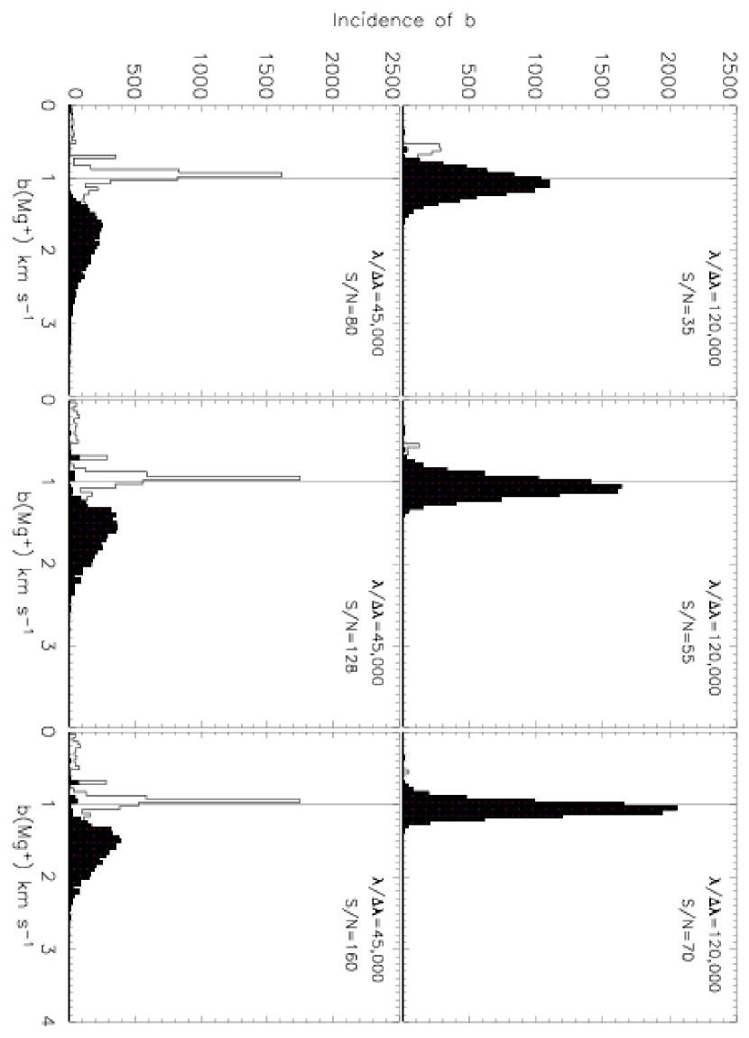
Figure 5: The distribution of measured Doppler parameter $b$ from $10,000$ realizations of an Mgii $\lambda 2796$ Å line with $W_{r}(2796)=0.02$ Å. The solid historgrams are measurements from well constrained Voigt Profile models that had $\sigma(b)<b$. For each case, the measurements that were affected by pixelization are separately shown as the unfilled histogram. The true value of $b$-parameter is $1.0$ km s^-1.

The real advantage of higher resolution is for even narrower lines. We performed a similar series of simulations for Mgii $\lambda$2796 lines with $N=10^{12}$ cm^-2 and $b=1$ km s^-1. The results for the distributions of $b$ parameters for various $S/N$ values at $R=120,000$ and $R=45,000$ are presented in Figure 5. The large spread in the measured value of $b$ for $R=45,000$ is indicative that this spectral resolution is inadequate to faithfully recover line widths of narrow line profiles. We again, for $R=45,000$ find a large number of measurements with large $\sigma(b)$ values, for measured $b$ of $\sim 0.95$ km s^-1. This is again explained by a pixelization effect, but in this case the measurement happens to be very close to the true value. Even if we had chosen a true value of $b$ between $1$ and $2$ km s^-1, this peak would still be at $b\sim 0.95$ km s^-1. Nonetheless, a measurement of a small $b$ value does imply a true narrow line–width, even if the measured value is biased by the pixelization.

Even for the $R=120,000$ spectra, the mode of the distribution for measured-$b$ is at a value slightly larger than the true $b$ although in general the measurements are well constrained. Table 1 lists the median values of Doppler parameters and column densities, and their $1$-$\sigma$ errors, for various $S/N$ values at the two resolutions. The distributions of $N$-values are compared in Figure 6.

The significance of increased resolution is clearly seen from Figures 3 through 6. The determination of $b$ is also sensitive to the sampling, where $b$ greater than roughly a pixel is required. In comparison, the precision in measurements from lower resolutions can be improved only by using substantially higher $S/N$ spectra thus requiring very long exposure time. Furthermore, we find that similar equivalent width limits are attained in the $R=120,000$ and $R=45,000$ spectrum for equal exposure lengths though the $S/N$ ratio of the former is substantially lower. For example, the $5\sigma$ equivalent width limit for $R=45,000$, $S/N=80$ and $R=120,000$, $S/N=35$ is $5$ mÅ/pixel. Also, as we discuss in the following sub-section and in § 3, observations with $R=120,000$, corresponding to a resolution of $2.5$ km s^-1, are very important for resolving lines and separating velocity sub-structures.

2.2 Blending of Lines

To probe the nature of small scale structure in absorbers it is essential to resolve closely separated velocity components. Here we focus on making estimates of the scale at which superhigh resolution offers a real improvement over intermediate resolution spectra. We chose a simple scenario of two absorbing clouds, with different physical properties, marginally separated in velocity. The column densities and Doppler parameters of the simulated lines were selected to match closely with those of the weak multiple cloud system at $z=1.0414$ in the spectrum of PG $1634+706$, so that our choice is not completely arbitrary. This multiple cloud system is discussed in § 3.3. The two components have column densities $N({\hbox{{\rm Mg}${}^{+}$}})$ of $10^{12}$ and $10^{11.5}$ cm^-2 and Doppler parameters $b({\hbox{{\rm Mg}${}^{+}$}})$ of 4.0 and 3.0 km s^-1, respectively. This corresponds to an equivalent width ratio of approximately $3:1$ between the two components. In a set of $1000$ simulations with a $S/N$ of $80$ pixel^-1 at $R=45,000$, and with the two clouds separated in velocity by $\Delta$v=10 km s^-1, we found that in $\sim 84\%$ of the cases Voigt Profile fitting was able to distinguish the two components in the absorption profile. For the same $S/N$ ratio, with the velocity separation reduced to $\Delta$v=7km s^-1, in $\sim 95\%$ of the cases the simulated line was fit with just a single broad Voigt profile with a mean value of $\bigl{<}b$(Mg⁺)$\bigl{>}=6.3$ km s^-1. This translates to a larger upper limit for the estimated temperature of the gas (T $<58000$ K) compared to the true value of T $<20000$ K. For lines with the same intrinsic properties, but simulated at $R=120,000$ and $S/N=35$ pixel^-1 (corresponding to an identical exposure time), we found that Voigt profile fits recovered both kinematic components in $\sim 97\%$ of the cases with a velocity separation of $\Delta$v=7 km s^-1, and in $100\%$ of the cases with the velocity separation increased to $\Delta$v=10 km s^-1. Furthermore, increasing the $S/N$ ratio of the intermediate resolution spectra did not compensate for the lower resolution. For example, when the two components were separated in velocity by $7$ km s^-1, even with $S/N=160$ pixel^-1 at $R=45,000$, the kinematically separate components were resolved only in $\sim 40\%$ of the cases. Figure 7 shows a sample of the simulated lines at the two resolutions. From these results we infer that even at fairly high $S/N$ ratios, intermediate resolutions can be completely inadequate in revealing closely blended velocity structures on scales smaller than $8$ km s^-1. Further, such unresolved lines can lead to overestimation of the temperature of the absorbing gas. More generally, we conclude that, if two lines are narrower than their velocity separation, they can be resolved by a Voigt profile fit if the resolution is less than $\sim 70$% of the velocity separation. The exact criterion for separating blends is dependant on the quality of the spectra and the Doppler parameters of the two lines.

2.3 Contribution from Isotopes and Hyperfine Splitting

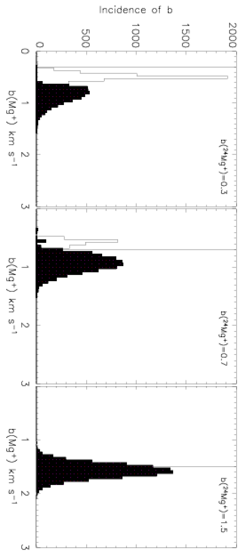
Figure 9: The distribution of measured Doppler parameter from 10,000 realizations of Mgii 2796 Å involving the isotopic and hyperfine lines of Magnesium. The unfilled histograms are measurements with poor constraints ($\sigma(b)>b$). The vertical line shows the true $b$-value assigned to ²⁴Mg⁺ in each of the three cases. The $b$ parameter is quoted in units of km s^-1.

Magnesium has three isotopes with mass numbers 24, 25 and 26 a.m.u, with relative abundances of $78.99\%$, $10.00\%$, $11.01\%$, respectively. The wavelengths of the resonance lines for these isotopes differ from one another. Furthermore, ²⁵Mg shows hyperfine splitting. The relative shifts in rest frame wavelength for each line of the resonance doublet are measured to be $\lambda_{24}-\lambda^{+}_{25}=0.0014$ Å, $\lambda_{24}-\lambda^{-}_{25}=0.0061$ Å, and $\lambda_{24}-\lambda_{26}=0.008$ Å (Morton, 2003). In velocity space this corresponds to $0.1500$ km s^-1, $0.6540$ km s^-1 and $0.8577$ km s^-1, respectively. For such narrow velocity separations, the effect of isotope shifts and hyperfine splitting becomes distinguishable only at extremely high spectral resolutions ($R>500,000$), as illustrated in Figure 8. To estimate the scale at which this effect is likely to influence our $b$-value measurements, we simulated very narrow synthetic lines with true $b({\hbox{${}^{24}${\rm Mg}${}^{+}$}})$ of 0.3, 0.7, and 1.5 km s^-1. The $b$-values of the other isotope lines were thermally scaled. The simulated lines had $S/N=35$ pixel^-1 at $R=120,000$. Figure 9 shows the dispersion in the incidence of measured $b$ for the various cases. Of the $10,000$ simulated lines with $b({\hbox{${}^{24}${\rm Mg}${}^{+}$}})=0.3$ km s^-1, only $\sim 10\%$ of the measurements yielded a $b$-value less than $0.5$ km s^-1, with the recovered $b$-value almost always larger than the true value. For a higher true $b$-value of $0.7$ km s^-1, the measurements were still distributed across a range from $0.7$ to $1.5$ km s^-1. The peak of this distribution, however, was closer to the true-value as compared to the previous case. For the final case, with $b=1.5$ km s^-1, the spectral resolution became adequate to repeatedly measure values close to the true $b$ value along with consistently yielding measurements that are reliable ($\sigma(b)<b$). In this case, although the isotope and hyperfine lines were still contributing to the final absorption profile, their contribution did not induce a significant change in the line width as the individual line widths were now larger than the largest separation between the isotope lines.

With these results we infer that isotopic line shifts and hyperfine splitting are to be considered as influencing our measurements only when the true line width is really narrow (T $<700$ K, $b({\hbox{{\rm Mg}${}^{+}$}})<0.7$ km s^-1). Furthermore, for such narrow Mgii lines, identifying the effect would require spectral resolutions of $R>500,000$.

3 SUPER HIGH RESOLUTION OBSERVATION OF PG $\mathbf{1634+706}$

We obtained a super high resolution spectrum of PG $1634+706$ with the High Dispersion Spectrograph (Noguchi et al., 1999, HDS) on Subaru. Using a 0.3″ slit width, we were able to attain $R=120,000$ spectrum with a sampling rate of $3$ pixels per resolution element. Our 1 hr observation yielded a spectrum with an average $S/N\sim 30$ pixel^-1 over the entire spectral range. The reduced $1$D spectrum was extracted in a standard manner with the IRAF software . Wavelength calibration was done using a standard Th–Ar spectrum. The spectrum was continuum fitted with a third–order cubic spline function and normalized. Previously identified weak and strong Mgii absorption systems in a $R=45,000$ Keck/HIRES spectrum of PG $1634+706$ made this observation an ideal test case. The HIRES data aquisition and reduction procedure is described in (Churchill et al., 2001). The short exposure on HDS reached an equivalent width limit several times smaller than our exposure of twice its length with the HIRES instrument at a lower resolution of $R=45,000$. Details of the two observations are listed in Table 2. Figures 10a–10c show the wavelength regions that are covered in both the HDS and HIRES spectrum.

In the following subsections, we compare detections of the strong, single cloud weak , and multiple cloud weak Mgii absorption features in the super-high resolution HDS and the high resolution HIRES spectra for this quasar. We also consider the Milky Way absorption along this line of sight. We discuss the particular case of these systems, but also generalize to discuss how studies of the same type of system would be affected by higher resolution observations. Since the scope of this paper is to compare observations taken at different spectral resolutions, we defer detailed analyses of the absorption-line systems presented herein to future work.

3.1 Strong Mgii absorber at $\mathbf{z=0.9902}$

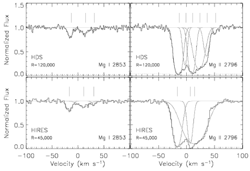
Figure 11: The $z=0.9902$ strong Mgii system as captured by the Keck/HIRES and Subaru/HDS spectrum of PG $1634+706$. The left panel shows the low ionization Mgi feature associated with this strong system. The thin solid line superimposed on the spectrum are the various Voigt Profile components contributing to the absorption feature. The tick marks placed above the features represent the center of each component. The dotted line is the error spectrum. The results from the Voigt Profile fit are listed in Table 3

The $z=0.9902$ system along the line of sight to the quasar PG $1634+706$ has previously been studied using a combination of the $R=45,000$ Keck/HIRES spectrum, data from HST/FOS (Churchill et al., 2000; Charlton et al., 2000) and from HST/STIS (Ding et al., 2003). Churchill et al. (2003) found that this strong Mgii doublet could be adequately fit with five blended components. With the higher resolving power of HDS, additional kinematic components were revealed in the Mgii absorption feature. Our Voigt profile fit decomposes the Mgii $\lambda\lambda 2796,2803$ profile into seven components. Figure 11 shows the HIRES and HDS data, comparing differences in the profile shapes for the two resolutions. The asymmetrical shapes for the Mgii$\lambda$2796 line at $\Delta v\sim 22$ km s^-1 and $\Delta v\sim 8$ km s^-1 from the flux–weighted system center in HIRES spectrum were indicative of narrowly blended features which are clearly distinguished in the profiles in the HDS spectrum. Table 3 presents our Voigt fitting parameters for Mgii $\lambda\lambda 2796,2803$ from the Keck/HIRES and the Subaru/HDS observations. This ability of superhigh resolution to resolve additional components in strong metal line absorbers was also noted by Chand et al. (2006).

Strong Mgii absorption systems usually have absorption from gas in different phases (different densities and temperatures) residing within an impact parameter of 35h^-1 kpc of a luminous galaxy with $L>0.05$ L^∗ (Bergeron & Boissé, 1991; Steidel et al., 1997). Dissecting the Mgii absorption profile to reveal kinematic structures at small velocity separations of $\Delta v<1$ km s^-1 is therefore useful in developing a physical understanding of the spatial distribution of gas in galaxies along the line of sight. If the observed Mgii absorption signatures are characteristic of disk ISM (Lanzetta & Bowen, 1992; Charlton & Churchill, 1998), then measuring structure on the smallest scales is important to determine if the interstellar medium of high redshift galaxies follows a complex fractal structure similar to Milky Way (e.g., Elmegreen, 1997). Resolving closely blended components, as in the $z\sim 0.9902$ system is also essential in developing ionization models that provide strong constraints on physical parameters. This is especially relevant when there is a difference or gradient in metallicity, abundance pattern or ionization from cloud to cloud.

Churchill et al. (2003) studied $23$ Mgii systems at $z\sim 1$ and found that many strong Mgii systems have observed column density ratios of N(Mg)/N(Mg⁺) $>0.01$. This value is the maximum expected if the absorption is taking place in gas at a single phase under photoionization equilibrium. In developing a model for this $z=0.9902$ absorption system based on the $R=45,000$ Keck/HIRES observations, Ding et al. (2003) found that the Mgi absorption line in this system is too strong to arise in the same phase as Mgii for all possible ionization parameters. To reconcile this discrepancy, Ding et al. (2003) invoked an additional lower ionization phase that gave rise to the majority of Mgi absorption, but which produced small amounts of Mgii. The lower ionization phase also produced most of the neutral hydrogen absorption from this system, with a range $17.3<\log N({\hbox{{\rm H}}})<17.7$ for the five Mgi clouds. In this model, the Mgi phase gas has a very low temperature ($T\sim 800$ K, $b\sim 0.75$ km s^-1), high density (n${}_{H}\sim 200$ cm^-3) and small size ($\sim 100$ AU), reminiscent of a cold pocket embedded in a warm, ionized inter-cloud medium as in the ISM of galaxies. The spectral resolution of HIRES was inadequate to show the narrow line widths that we might expect from such cold, small-scale clumps of gas. However, the present Subaru/HDS spectrum provides a direct test of the Ding et al. (2003) prediction for this $z=0.9902$ absorber.

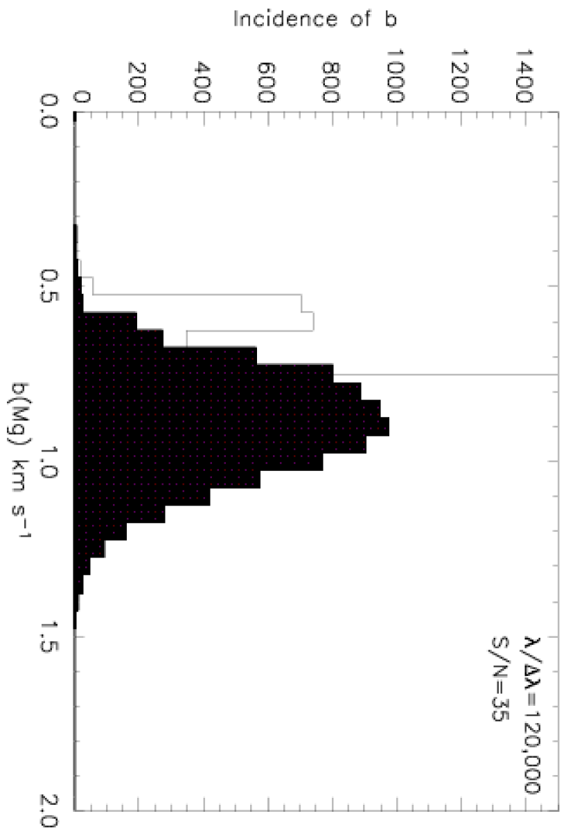
Figure 12: The distribution of measured $b$ parameter from 10,000 realization of Mgi 2853 Å by considering the isotopic lines of Magnesium. The unfilled histogram includes measurements that yielded poor constraints($\sigma(b)>b$). The vertical line shows $b({\hbox{${}^{24}${\rm Mg}}})=0.75$ km s^-1, which is the true Doppler parameter for that line. The line was chosen to have a column density of $N({\hbox{{\rm Mg}}})=10^{11.1}$ cm^-2 to match with the model predicted by (Ding et al., 2003).

Figure 12 shows the absorption from Mgi $\lambda$2853 in the $z=0.9902$ system, as seen in the HDS spectrum. The Voigt profile fit constraints on the various line features is listed in Table 3. For the three clouds used to fit the Mgi profile, the line widths are not as small as what Ding et al. (2003) had predicted in their models (see their Table 1). For the line width predicted by their model, the Mgi absorbption has to be from gas at temperature $T<800$ K. Our simulation results from § 2.3 show that in instances where the true-$b$ value is very small, Voigt profile measurements can yield higher values because of unresolved isotopic lines. To investigate if our measurements of $b$-value for the various components of Mgi is influenced by this effect, we resort to simulations. The isotopic lines of Mgi occur at $\lambda_{24}=2852.9635$ Å, $\lambda_{25}=2852.9655$ Å and $\lambda_{26}=2852.9674$ Å (Beverini et al., 1990). The Mgi $2853$ Å line does not have hyperfine structure. In our simulations, we used the profile parameters predicted by the model (N(Mg)=$10^{11.1}$ cm^-2, $b({\hbox{{\rm Mg}}})=0.75$ km s^-1) for the isotopic line of ²⁴Mg, with the $b$-parameters of the other two isotopic lines thermally scaled. The spectra were simulated for a $S/N=35$ pixel^-1 at $R=120,000$, with the lines redshifted to match the redshift of the system. Figure 12 shows the distribution in the incidence of measured $b$ from a simulation of $1000$ lines. It can easily be noticed that, although the measured $b$ is almost always larger than the true $b$ of $0.75$ km s^-1, a measurement of $2$ km s^-1 or higher (as in the observed HDS spectrum) never occurs. It is therefore to be concluded that the hypothesis of a two phase structure as an explanation of the Mg to Mg⁺ ratio is therefore not consistent with the high resolution observations. It is clear from § 2 that a component with $b=0.75$ km s^-1 will not be measured to have $b$ as high as several km s^-1 at $R=120,000$. Therefore, another explanation must be sought for this system. Tappe & Black (2004) suggested that a UV flux contribution from the absorbing galaxy and/or Mg $+$ H⁺ charge transfer could significantly influence the Mg to Mg⁺ ratio. Their $R=100,000$ VLT/UVES observation of a different system, at $z=0.79089$ toward PKS $2145+067$, yield $b({\hbox{{\rm Mg}${}^{+}$}})=1.02\pm 1.65$ km s^-1 for the one component detected in Mgi in a spectral region with $S/N\sim 30$. The error is too large to draw a conclusion in that case. Another possibility for the $z=0.9902$ system is that there are more components in the Mgi than we are able to resolve.

We conclude that our $R=120,000$ spectrum does not provide support for a cold phase model for the $z=0.9902$ system, though some modified version could apply. Direct tests with super high resolution for other similar systems are needed. One excellent candidate is the $z=0.4523$ multiple-cloud, weak Mgii system toward the quasar HE $0001-2340$ ($z=2.28,m_{V}=16.7$), which has detected Fei, and Cai as well as Mgi (Jones et al., 2006). Cold phase models may also have significant consequences for the study of damped Lya absorbers (DLAs) and sub-DLAs. Lane et al. (2000) have resolved narrow components ($b\sim 2-3$ km s^-1) in an Hi $21$cm study of the DLA system at $z=0.0912$ toward B $0738+313$. Mgi lines in these systems are expected, from thermal scaling, to be significantly narrower. Also, more recently, Srianand et al. (2005) report measuring kinetic temperature of $\sim 150$ K from H₂ lines in three DLAs. Such a low gas phase temperature can produce narrow metal lines, with Doppler width of $\sim 3$ km s^-1, that can be accurately recovered with superhigh resolution spectra. A fair fraction of DLAs have detected molecules (e.g., Petitjean et al., 2000) , indicating directly that they have a cold phase. Other DLAs and Lyman limit systems may also be produced by lines of sight through cold regions surrounding molecular clouds, or regions that did not quite reach the threshold for star formation.

3.2 Single-Cloud Weak Mgii absorbers

Most single-cloud, weak Mgii absorbers (rest–frame equivalent width $W_{r}(2796)<0.3$ Å) are not associated with luminous galaxies, although models designed to fit the Lyman series line and the observed lack of Lyman break constrain the metallicity of the absorbing gas to be at least 10$\%$ solar. Photoionization models suggest that the structures responsible for weak Mgii absorption might be unstable over astronomical timescales, because of pressure imbalance between a high density, low ionization ($p/k=10^{-5}$ cm^-3 K^-1) and a low density high ionization ($p/k=10^{-8}$ cm^-3 K^-1) phase (Charlton et al., 2003; Narayanan et al., 2005). The conclusions from photoionization models are based on the observed values of column density and Doppler parameter for the low and high ionization transitions. The best constraints on these parameters were mostly from high resolution data at $R\sim 45,000$ or lower. The $b$ parameters measured at $R\sim 45,000$ ($b\sim 2$ or $3$ km s^-1) allowed for temperatures of thousands of Kelvin, similar to the temperatures inferred for the high ionization phases. If the true Doppler parameter is smaller than that derived from the HIRES measurements, then it would imply that the low ionization phase has a much lower temperature than the high ionization phase. This influences the inference about their stability. Line widths narrower than $\sim 2$ km s^-1 ($T<15,000$ K) cannot be accurately measured at $R=45,000$. Therefore the temperature estimations for the low ionization phase in these absorbers may not be accurate. Our $R=120,000$ Subaru/HDS spectrum allows us to test the assumption that these single-cloud weak Mgii lines are resolved.

For the two single cloud weak Mgii absorbers at $z=0.9056$ and $z=0.8181$ found in the PG $1634+706$ spectrum, we find from the HDS spectrum that the weak Mgii lines are not any narrower than values measured at R $45,000$ (Figures 13). The column densities and Doppler parameters from simultaneous Voigt profile fits to Mgii $\lambda\lambda 2796,2803$ are listed in Table 4. Thus at least for these cases, the lines were already sufficiently resolved at $R=45,000$ to allow measurements of the $b$-values that were accurate within the errors. These measurements are in concordance with the instability inference based on photoionization model. Analogs of weak Mgii absorbers are known to exist in the present day universe (Narayanan et al., 2005) as well as at intermediate ($z\sim 1$, Churchill et al., 1999) and higher redshifts ($z\sim 2$, Lynch et al., 2006). Therefore confirming the transient nature of these systems is significant in addressing the question of the evolution of the processes that created these absorbing structures. A larger sample of weak Mgii absorbers should be measured with super high resolution in order to verify that we can generalize this conclusion. However, the real value in $R>100,000$ observations in the study of weak Mgii absorbers will be the enhanced sensitivity which will allow us to establish the shape of the distribution function for the weakest absorbers, and to infer their physical properties.

3.3 Multiple-Cloud Weak Mgii absorbers

Approximately 35$\%$ of weak Mgii absorbers have multiple clouds (Rigby et al., 2002). Based on their kinematics, these multiple-cloud, weak Mgii absorbers can be described as “kinematically compact” or “kinematically spread”. The kinematically compact systems have been hypothesized to arise in dwarf galaxies, and the kinematically spread systems in the outskirts of spiral galaxies (Masiero et al., 2005; Ding et al., 2005), but it is likely that the situation is more complicated. Varying degrees of line blending in the absorption features implies that the Voigt profile fit results are sometimes going to be sensitive to resolution. This is illustrated by the $z=1.0414$ multiple-cloud, weak Mgii system in the spectrum of PG $1634+706$. Based on HIRES data, this weak Mgii absorber was classified as a multiple cloud weak Mgii system with $4$ discrete Mgii clouds (Churchill et al., 2003). Two additional weak components were resolved in Voigt profile fits to the higher resolution data in the same region, as shown in Figure 14. Zonak et al. (2004) produced models for the system based on the HIRES data along with $R=30,000$ ultraviolet spectra obtained with HST/STIS. It is apparent from our HDS spectrum, in Figure 15, that there are two subsystems in Mgii, separated by $\sim 150$ km s^-1. For the blueward subsystem (see Zonak et al., 2004), Mgii $\lambda$2796 was not covered in the HIRES spectrum, and Mgii $\lambda$2803 was not detected, but several other metal-line transitions (e.g. Siiii $1207$, Siiv $\lambda\lambda 1394,1403$ etc) were detected in the HST/STIS spectrum. The greater sensitivity of the $R=120,000$ HDS spectrum led to detection of Mgii $\lambda$2803 in the blueward subsystem, which was a prediction of the models of Zonak et al. (2004)

Enhanced resolution allows the detailed shapes of absorption profiles to be surveyed, and blends to be separated. Some single-cloud weak Mgii absorbers appear asymmetric when observed at $R=45,000$ (Churchill et al., 1999), suggesting they may have more than one Voigt profile component. More generally, it is of interest what fraction of the single-cloud weak Mgii absorbers are truly fit by single Voigt profile components when viewed at higher resolution. The profiles of the $z=0.9056$ and $z=0.8181$ systems observed at $R=120,000$ here, still are fit adequately by a single component, suggesting a very simple structure. Observing some asymmetric single-cloud weak Mgii may reveal some to be more similar to kinematically compact multiple cloud weak Mgii absorbers, or they could just be variations of ordinary single-cloud weak Mgii absorbers. Determinations of their metallicities and comparisons of kinematics of other transitions should allow a separation of these classes.

3.4 Milky Way Absorption and High Velocity Clouds

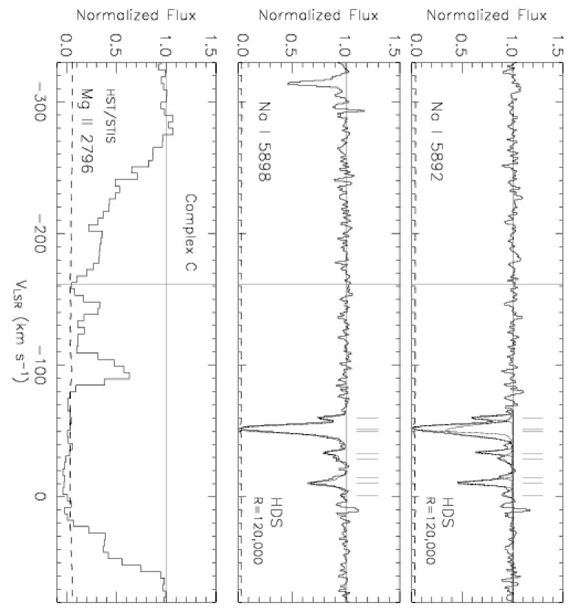
Figure 16: Galactic Nai detections in the HDS spectrum of PG $1634+706$. The superhigh resolution spectrum allowed measurements of $b$-value $\sim 1$ km s^-1. Superimposed in thin lines are the various Voigt Profile components contributing to the absorption. The vertical ticks mark the center of each component. The thin line in the Nai 5898 panel shows the cumulative Voigt Profile by combining the various components. The fit results are listed in Table 5. The Mgii absorption from the HVC Complex C along the line of sight to the quasar is also shown. To guide the eye, the expected location of the Nai doublet absorption from the HVC is marked by the vertical line.

In the HDS spectrum, Galactic Nai is detected, as shown in Figure 16. Voigt profile fitting parameters are listed in Table 5. For the narrowest component, at $v_{LSR}=-32$ km s^-1 we measure $b=0.9\pm 0.2$ km s^-1. This shows that such narrow lines as $b\sim 1$ km s^-1 can be measured at $R=120,000$. At the same time, we also note that the hyperfine splitting in Nai lines are likely to affect our measurement of such a narrow line width. The difference in rest-frame wavelength from the basic hyperfine splitting of the D1 and D2 lines has been measured to be $0.0213$ Å and $0.0198$ Å, respectively (Morton, 2003). This corresponds to shifts in velocity of $1.0827$ km s^-1 and $1.0075$ km s^-1, respectively. As these values are very close to our measurement of $b\sim 1$ km s^-1, we expect the true-$b$ to be lower than this measured value. However, observing this effect by resolving the line would require spectral resolutions that are significantly larger than our HDS measurement at $R=120,000$ (as discussed in § 2.2.)

The PG $1634+706$ line of sight passes through the well-studied high velocity cloud complex C. Upon inspection of a HST/STIS E230M spectrum, we find absorption detected in Mgii, Mgi, and Feii at $v_{LSR}\sim-115$ and $-155$ km s^-1. We do not detect Nai$\lambda\lambda$5892,5898 at these velocities in our $R=120,000$ spectrum to a $3\sigma$ limit of $0.004$ Å pixel^-1. Recently, $21$cm Hi observations have found that high velocity, low column density hydrogen clumps have T $<900$ K (Hoffman et al., 2004; Richter et al., 2005) and that narrow Caii lines are detected in most sightlines (Richter et al., 2005). Unfortunately, Caii$\lambda\lambda$3935,3970 is not covered in either our $R=45,000$ or $R=120,000$ spectrum of PG $1634+706$. However, at $R=45,000$, it would not be possible to test if the Caii lines are as narrow as would be suggested by the low temperatures from Hi. Thus the study of HVCs is an application for which super-high resolution will be particularly valuable. This applies to HVCs around galaxies at high redshift as well as to Milky Way HVCs.

4 CONCLUSION

The ability to routinely obtain quasar spectra with resolutions of $R>100,000$ is not likely to provide as large a change in the field of quasar absorption lines as the previous advance to $R=45,000$, made possible with $8$–meter class telescopes. However, the ability to probe structure on scales of $\sim 1$ km s^-1 will certainly be valuable in select applications and in detailed studies of particular absorbers. Examples of such applications include probing the physical conditions of cold regions in the ISM of galaxies, particularly in DLAs and other strong Mgii absorbers. Also, it appears that high velocity clouds, both around the Milky Way and at high redshift, may have a cold phase. Finally, surveys extending to small equivalent widths will be aided by the enhanced sensitivity of higher resolution observations.

Our comparison of $R=120,000$ Subaru/HDS observations to $R=45,000$ Keck/HIRES observations of various systems toward PG $1634+706$ show that at the higher resolution, more accurate Doppler parameter measurements can be made, and that additional Voigt profile components are resolved. However, for the particular Mgii absorbers along the PG $1634+706$ sightline no extremely narrow individual components were measured. It was only for the Galactic Nai line in this line of sight that $b<1$ km s^-1 was measured. Because such narrow components are expected in a variety of environments, it would be valuable to push the limits of 8-meter class telescopes in order to detect them in a variety of types of systems toward the brightest quasars.

We are grateful to Chris Churchill for giving us permission to use the Keck/HIRES spectrum for this work. We also wish to thank the referee, John Black, for several insightful comments that have increased the scope of this paper.

Figure 2: A sample from our synthetically simulated Mgii $\lambda$2796 Å absorption lines with noise added. The two set of lines with Doppler parameters $b({\hbox{{\rm Mg}${}^{+}$}})=2.0$ km s^-1 and $b({\hbox{{\rm Mg}${}^{+}$}})=1.0$ km s^-1 have a column density of $N({\hbox{{\rm Mg}${}^{+}$}})=10^{12}$ cm^-2. The dotted line in each panel is the error spectrum. The tick marks represent the center of each absorption profile.

Figure 3: The distribution of measured Doppler parameter $b$ from $10,000$ realizations of an Mgii $\lambda 2796$ Å line with $W_{r}(2796)=0.03$ Å. The solid historgrams are measurements from well constrained Voigt Profile models that had $\sigma(b)<b$. For each case, the measurements that were affected by pixelization are separately shown as the unfilled histogram. The true value of $b$-parameter is $2.0$ km s^-1

Figure 4: The distribution of measured $N({\hbox{{\rm Mg}${}^{+}$}})$ column density from $10,000$ realizations of the Mgii $\lambda 2796$ Å line with $W_{r}(2796)=0.03$ Å. The true value of column density is $N({\hbox{{\rm Mg}${}^{+}$}})=10^{12}$ cm^-2.

Figure 6: The distribution of measured $N({\hbox{{\rm Mg}${}^{+}$}})$ column density from $10,000$ realizations of the Mgii $\lambda 2796$ Å line with $W_{r}(2796)=0.02$ Å. The histogram shown in dotted line are measurements that yielded poor constraints ($\sigma(b)>b$). The true value of column density is $N({\hbox{{\rm Mg}${}^{+}$}})=10^{12}$ cm^-2.

Figure 7: A sample showing closely blended synthetically simulated Mgii 2796 Å lines with noise added corresponding to a $S/N$ ratio. The sub-panels in the left panel correspond to the two absorbing components separated in velocity by $10$ km s^-1. The right panel are sample simulated spectra illustrating the case where the two absorbing components are separated in velocity by $7$ km s^-1. The ticks mark the position of the two components. The $S/N$ ratio for the two resolutions are estimated for equal exposure times.

Figure 8: Synthetic spectra involving isotope and hyperfine lines, without adding Poisson noise. The Mgii line is redshifted to $z=1$. A column density of $N({\hbox{{\rm Mg}${}^{+}$}})=10^{11.5}$ cm^-2 was assumed. The $b$ parameter is quoted in units of km s^-1. The line asymmetry because of isotopic line shift becomes distinguishable at spectral resolution $R>500000$ and also when the Doppler width is smaller.

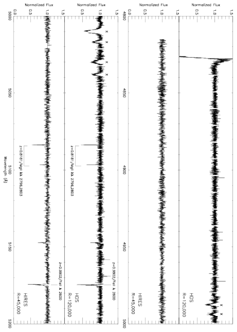
Figure 10a: Comparison of PG $1634+706$ observations using $R=120,000$ Subaru/HDS and $R=45,000$ Keck/HIRES. The details of the observation are listed in Table 1. The metal lines associated with the absorption systems discussed in this paper are identified and labelled in both spectrum. The features in the HDS spectrum marked with ’x’ are unreal and were produced by bad regions in the CCD.

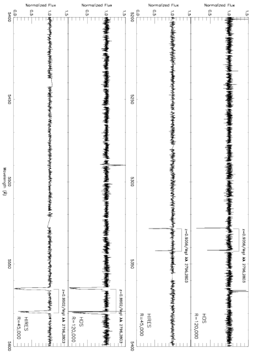
Figure 10b: Contd. Figure 10a

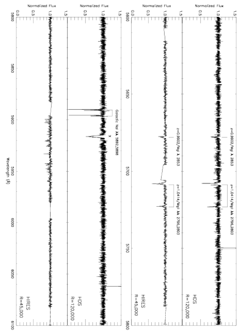
Figure 10c: Contd. Figure 10a

Figure 13: The two single–cloud weak Mgii systems at redshifts 0.8181 (left panel) and 0.9056 (right panel) as detected in the Keck/HIRES and Subaru/HDS spectrum of PG $1634+706$. The dotted line is the error spectrum. The Voigt Profile fit results are listed in Table 4

Figure 14: The multiple–cloud weak Mgii system at $z=1.0414$ as detected in the Keck/HIRES and Subaru/HDS spectrum of PG $1634+706$. The thin solid line superimposed on the spectrum are the various Voigt Profile components contributing to the absorption feature. The tick marks placed above the features represent the center of each component in the absorption profile. The dotted line represents the error spectrum. The Voigt Profile fitting results are listed in Table 4

Figure 15: The $z=1.0414$ multiple–cloud weak Mgii system and the associated subsystem in the spectrum of PG $1634+706$. The dotted line represents the error spectrum. The thin solid lines mark the respective positions for the $\lambda$$\lambda$ 2796 Å and 2803 Å lines that form the doublet pair. The two absorption systems are separated by $\sim 150$ km s^-1. In the HIRES spectrum, for the bluer subsystem, Mgii $\lambda 2796$ transition was not covered due to an echelle order break. However, the weaker pair of the doublet, Mgii $\lambda 2803$, was not detected down to an equivalent-width limit of $3\sigma$. However, there is a clear detection of this weak subsytem in the HDS spectrum.

Table 1: Results from simulations

$R/1000$	$S/N$ ratio	$b({\hbox{{\rm Mg}${}^{+}$}})=2.0$ km s-1			$b({\hbox{{\rm Mg}${}^{+}$}})=1.0$ km s-1
	pixel-1	$b({\hbox{{\rm Mg}${}^{+}$}})^{*}$	$\log$ $N({\hbox{{\rm Mg}${}^{+}$}})^{*}$	% Models †	$b({\hbox{{\rm Mg}${}^{+}$}})^{*}$	$\log$ $N({\hbox{{\rm Mg}${}^{+}$}})^{*}$	% Models †
$120$	$35$	$2.02_{-0.14}^{+0.15}$	$12.0_{-0.02}^{+0.02}$	$99.99$	$1.07_{-0.16}^{+0.16}$	$11.97_{-0.04}^{+0.06}$	$90.21$
$45$	$80$	$2.15_{-0.48}^{+0.43}$	$11.99_{-0.03}^{+0.04}$	$94.33$	$1.82_{-0.33}^{+0.44}$	$11.84_{-0.03}^{+0.04}$	$44.00$
$120$	$55$	$2.02_{-0.09}^{+0.10}$	$12.0_{-0.02}^{+0.01}$	$99.98$	$1.05_{-0.13}^{+0.11}$	$11.97_{-0.03}^{+0.05}$	$97.80$
$45$	$128$	$2.17_{-0.32}^{+0.26}$	$11.98_{-0.01}^{+0.03}$	$98.44$	$1.56_{-0.27}^{+0.35}$	$11.85_{-0.02}^{+0.04}$	$51.86$
$120$	$70$	$2.02_{-0.07}^{+0.08}$	$12.0_{-0.01}^{+0.01}$	$99.98$	$1.05_{-0.10}^{+0.09}$	$11.97_{-0.02}^{+0.04}$	$98.98$
$45$	$160$	$2.17_{-0.25}^{+0.21}$	$11.98_{-0.01}^{+0.02}$	$98.03$	$1.55_{-0.28}^{+0.33}$	$11.86_{-0.03}^{+0.03}$	$51.98$

Note. — ^∗ Median $b$ and $N$ values.

^† - Out of 10,000 realizations, the percentage of Voigt Profile fit models that gave a reliable measurement ($\sigma(b)<b$).

Table 2: PG $1634+706$ Observations; $z_{\textrm{\scriptsize QSO}}$=$1.337$, $m_{V}$=14.9.

Instrument	Resolution	${\triangle}v$	Date(s) of	Texp	Coverage	PI
	$\lambda$/${\triangle}\lambda$	km s-1	Observation	seconds	$\lambda$ Å
Keck/HIRES	$45,000$	$6.6$	$1994$ Jul $04$	$2700$	$3723-6185$	Churchill
	$45,000$	$6.6$	$1994$ Jul $05$	$5400$	$3723-6185$	Churchill
Subaru/HDS	$120,000$	$2.5$	$2005$ Jun $06$	$3600$	$4830-7560$	Misawa

Table 3: Voigt Profile Fit Results for $z=0.9902$ Strong Mgii System

Instrument	$v$	$\log$ $N$	$b$
	km s-1	atoms cm-2	km s-1
Mgi Fit Results
HIRES	$-22.6$	$11.35~{}{\pm}~{}0.04$	$6.52~{}{\pm}~{}0.71$
	$5.2$	$11.37~{}{\pm}~{}0.06$	$13.52~{}{\pm}~{}2.44$
	$25.0$	$10.65~{}{\pm}~{}0.18$	$3.2~{}{\pm}~{}2.52$
HDS	$-20.1$	$11.26~{}{\pm}~{}0.03$	$5.87~{}{\pm}~{}0.46$
	$7.7$	$11.28~{}{\pm}~{}0.04$	$10.55~{}{\pm}~{}1.28$
	$24.5$	$10.51~{}{\pm}~{}0.10$	$5.87~{}{\pm}~{}0.94$
Mgii Fit Results
HIRES	$-22.1$	$13.04~{}{\pm}~{}0.01$	$7.72~{}{\pm}~{}0.09$
	$1.1$	$12.82~{}{\pm}~{}0.01$	$4.11~{}{\pm}~{}0.12$
	$8.3$	$13.30~{}{\pm}~{}0.01$	$22.29~{}{\pm}~{}0.21$
HDS	$-20.2$	$13.05~{}{\pm}~{}0.01$	$7.57{\pm}~{}0.15$
	$-8.2$	$12.44~{}{\pm}~{}0.06$	$4.46~{}{\pm}~{}0.48$
	$3.8$	$12.90~{}{\pm}~{}0.22$	$6.50~{}{\pm}~{}1.00$
	$16.8$	$12.93~{}{\pm}~{}0.34$	$11.03~{}{\pm}~{}8.00$
	$30.1$	$12.34~{}{\pm}~{}0.55$	$6.11~{}{\pm}~{}1.91$
	$45.4$	$11.34~{}{\pm}~{}0.09$	$3.37~{}{\pm}~{}0.69$

Table 4: Voigt Profile Fit Results for Weak Mgii Systems

Instrument	$v$	$\log$ [$N({\hbox{{\rm Mg}${}^{+}$}})$]	$b({\hbox{{\rm Mg}${}^{+}$}})$
	km s-1	atoms cm-2	km s-1
$z=0.8181$ single–cloud system
HIRES	$0$	$12.04~{}{\pm}~{}0.03$	$2.14~{}{\pm}~{}0.40$
HDS	$0$	$11.97~{}{\pm}~{}0.02$	$2.61~{}{\pm}~{}0.13$
$z=0.9056$ single–cloud system
HIRES	$0$	$12.47~{}{\pm}~{}0.01$	$2.77~{}{\pm}~{}0.12$
HDS	$0$	$12.42~{}{\pm}~{}0.01$	$3.14~{}{\pm}~{}0.07$
$z=1.0414$ multiple–cloud system
HIRES	$-38.2$	$11.49~{}{\pm}~{}0.08$	$6.53~{}{\pm}~{}1.62$
	$-15.2$	$11.90~{}{\pm}~{}0.06$	$10.81~{}{\pm}~{}2.03$
	$0$	$12.02~{}{\pm}~{}0.03$	$3.12~{}{\pm}~{}0.38$
	$15.7$	$11.68~{}{\pm}~{}0.04$	$5.95~{}{\pm}~{}0.83$
HDS	$-36.4$	$11.17~{}{\pm}~{}0.23$	$3.98~{}{\pm}~{}2.78$
	$-29.6$	$10.98~{}{\pm}~{}0.27$	$2.23~{}{\pm}~{}1.46$
	$-17.3$	$11.38~{}{\pm}~{}0.14$	$5.19~{}{\pm}~{}1.99$
	$-10.1$	$11.05~{}{\pm}~{}0.25$	$2.35~{}{\pm}~{}1.08$
	$1.9$	$12.02~{}{\pm}~{}0.01$	$3.82~{}{\pm}~{}0.13$
	$18.0$	$11.48~{}{\pm}~{}0.04$	$2.86~{}{\pm}~{}0.34$

Table 5: Voigt Profile Measurement of Galactic Nai absorption in the HDS spectrum of PG $1634+706$

$v_{LSR}$	$\log$ [$N$(Na)]	$b$ (Na)
km s-1	atoms cm-2	km s-1
$-1.1$	$10.56~{}{\pm}~{}0.10$	$1.68~{}{\pm}~{}0.82$
$-10.0$	$11.51~{}{\pm}~{}0.02$	$1.63~{}{\pm}~{}0.16$
$-14.4$	$10.67~{}{\pm}~{}0.10$	$0.89~{}{\pm}~{}0.88$
$-28.6$	$10.90~{}{\pm}~{}0.11$	$2.80~{}{\pm}~{}1.02$
$-33.2$	$11.14~{}{\pm}~{}0.05$	$0.90~{}{\pm}~{}0.33$
$-49.9$	$11.96~{}{\pm}~{}0.34$	$4.64~{}{\pm}~{}0.28$
$-51.7$	$14.21~{}{\pm}~{}1.63$	$1.02~{}{\pm}~{}0.35$
$-59.6$	$11.26~{}{\pm}~{}0.05$	$0.86~{}{\pm}~{}0.21$

References

- Bergeron & Boissé (1991) Bergeron, J., & Boissé, P. 1991, AA, 243,344
- Beverini et al. (1990) Beverini, N., Maccioni, E., Pereira, D., Strumia, F., Vissani, G., & Wang, Y.-Z. 1990, Optics Communications, 77, 299
- Caulet (1989) Caulet, A. 1989, ApJ, 340, 90
- Chand et al. (2006) Chand, H., Srianand, R., Petitjean, P., Aracil, B., Quast, R., & Reimers, D. 2006, AA, 451, 45
- Charlton & Churchill (1998) Charlton, J. C., & Churchill, C. W. 1998, ApJ, 499, 181
- Charlton et al. (2003) Charlton, J. C., Ding, J., Zonak, S. G., Churchill, C. W., Bond, N. A., & Rigby, J. R. 2003, ApJ, 589, 111
- Charlton et al. (2000) Charlton, J. C., Mellon, R. R., Rigby, J. R., & Churchill, C. W. 2000, ApJ, 545, 635
- Churchill (1997) Churchill, C. W. 1997, Ph.D. Thesis, University of Santa Cruz
- Churchill et al. (2000) Churchill, C. W., Mellon, R. R., Charlton, J. C., Jannuzi, B. T., Kirhakos, S., Steidel, C. C., & Schneider, D. 2000, ApJ, 543, 577
- Churchill et al. (1999) Churchill, C. W., Rigby, J. R., Charlton, J. C., & Vogt, S. S. 1999, ApJS, 120, 51
- Churchill et al. (2001) Churchill, C. W., & Vogt, S. S. 2001, AJ, 122, 679
- Churchill et al. (2003) Churchill, C. W., Vogt, S. S., & Charlton, J. C. 2003, AJ, 125, 98
- Cowie et al. (1995) Cowie, L. L., Songaila, A., Kim, T.-S., & Hu, E. M. 1995, AJ, 109, 1522
- Davé et al. (1996) Davé, R., Hernquist, L., Katz, N., Weinberg, D., & Churchill, C. W. 1996, AAS, 188.2308D
- Dekker et al. (2000) Dekker, H., et al. 2000, SPIE, 4008, 534
- Ding et al. (2003) Ding, J., Charlton, J. C., Bond, N. A., Zonak, S. G., & Churchill, C. W. 2003, ApJ, 587, 551
- Ding et al. (2005) Ding, J., Charlton, J. C., & Churchill, C. W. 2005, ApJ, 621, 615
- Elmegreen (1997) Elmegreen, B. G. 1997, ApJ, 477, 196
- Fox et al. (2005) Fox, A. J., Wakker, B. P., Savage, B. D., Tripp, T. M., Sembach, K. R., & Bland-Hawthorn, J. 2005, ApJ, 630, 332
- Hoffman et al. (2004) Hoffman, G. L., Salpeter, E. E., & Hirani, A. 2004, AJ, 128, 2932
- Jones et al. (2006) Jones, T., Narayanan, A., Mshar, A., & Charlton, J. C. 2006, in preparation
- Kerr & Lynden-Bell (1986) Kerr, F. J., & Lynden-Bell, D. 1986, MNRAS, 221, 1023
- Lane et al. (2000) Lane, W. M., Briggs, F. H., & Smette, A. 2000, ApJ, 532, 146
- Lanzetta & Bowen (1992) Lanzetta, K. M., & Bowen, D. V. 1992, ApJ, 391, 48
- Lanzetta et al. (1987) Lanzetta, K. M., Turnshek, D. A., & Wolfe, A. M. 1987, ApJ, 322, 739
- Lynch et al. (2006) Lynch, R. S., Charlton, J. C., Kim, T. S. 2006, ApJ, 640, 81
- Masiero et al. (2005) Masiero, J. R., Charlton, J. C., Ding, J., Churchill, C. W., Kacprzak, G. 2005, ApJ, 623, 57
- Misawa et al. (2002) Misawa, T., Tytler, D., Iye, M., Storrie-Lombardi, L. J., Suzuki, N., & Wolfe, A. M. 2002, AJ, 123, 1847
- Morton (2003) Morton, D. C. 2003, ApJS, 149, 205
- Narayanan et al. (2005) Narayanan, A., Charlton, J. C., Masiero, J. R., & Lynch, R. 2005, ApJ, 632, 92
- Noguchi et al. (1999) Noguchi, K., et al. 1999, PASJ, 54, 855
- Petitjean et al. (2000) Petitjean, P., Srianand, R., & Ledoux, C. 2000, AA, 364, 26
- Points et al. (2004) Points, S. D., Lauroesch, J. T., & Meyer, D. M. 2004, PASP, 116, 801
- Richter et al. (2005) Richter, P., Westmeier, T., & Bru̇ns, C. 2005, AA, 442L, 49
- Rigby et al. (2002) Rigby, J. R., Charlton, J. C., & Churchill, C. W. 2002, ApJ, 565, 743
- Sargent et al. (1988) Sargent, W. L. W., Boksenberg, A., & Steidel, C. C. 1988, ApJS, 68, 539
- Sembach (2002) Sembach, K. R. 2002, ASPC, 254, 283 (astro-ph/0108088)
- Srianand et al. (2005) Srianand, R., Petitjean, P., Ledoux, C., Ferland, G., & Shaw, G. 2005, MNRAS, 362, 549
- Steidel et al. (1997) Steidel, C. C., Dickinson, M., Meyer, D. M., Adelberger, K. L., & Sembach, K. R. 1997, ApJ, 480, 568
- Tappe & Black (2004) Tappe, A., & Black, J. H 2004, AA, 423, 943
- Vogt et al. (1994) Vogt, S. S., et al. 1994, Proc.SPIE, 2198, 362
- Wolfe et al. (2003) Wolfe, A, M., Prochaska, J. X., & Gawiser, E. 2003, ApJ, 593, 215
- Zonak et al. (2004) Zonak, S. G., Charlton, J. C., Ding, J., & Churchill, C. W. 2004, ApJ, 606, 196