The isocurvature fraction after WMAP 3–year data

Abstract

I revisit the question of the adiabaticity of initial conditions for cosmological perturbations in view of the 3–year WMAP data. I focus on the simplest alternative to purely adiabatic conditions, namely a superposition of the adiabatic mode and one of the 3 possible isocurvature modes, with the same spectral index as the adiabatic component.

I discuss findings in terms of posterior bounds on the isocurvature fraction and Bayesian model selection. The Bayes factor (models likelihood ratio) and the effective Bayesian complexity are computed for several prior ranges for the isocurvature content. I find that the CDM isocurvature fraction is now constrained to be less than about $10\%$, while the fraction in either the neutrino entropy or velocity mode is below about $20\%$. Model comparison strongly disfavours mixed models that allow for isocurvature fractions larger than unity, while current data do not allow to distinguish between a purely adiabatic model and models with a moderate (i.e., below about $10\%$) isocurvature contribution.

The conclusion is that purely adiabatic conditions are strongly favoured from a model selection perspective. This is expected to apply in even stronger terms to more complicated superpositions of isocurvature contributions.

1 Introduction

The detailed nature of the initial conditions for cosmological perturbations is one of the open questions in cosmology. The exquisite precision of the WMAP measurement of the first acoustic peak location in the cosmic microwave background (CMB) temperature power spectrum ($\ell=220.7\pm 0.7$, see Hinshaw et al. (2006)) is a strong indication in favour of adiabatic initial conditions, which predict for the first peak $\ell\approx 220$. The alternative possibility of cold dark matter (CDM) isocurvature initial conditions excites a sine wave (rather than the cosine excited by adiabatic conditions) in the photon–baryon plasma, resulting in a first acoustic peak displaced by half a period to $\ell\approx 330$, see e.g. Trotta (2004); Durrer (2004). Furthermore, the ratio of the Sachs–Wolfe plateau for $\ell\,\raise 1.72218pt\hbox{$<$}\kern-8.00003pt\lower 2.6694pt\hbox{$\sim$}\,50$ to the height of the peak is very different for the two modes.

A few years ago, Bucher and collaborators introduced two new isocurvature modes, called “neutrino density” (or, more appropriately, “neutrino entropy”) and “neutrino velocity” modes (Bucher et al., 2000). They are characterized by a non–vanishing initial entropy perturbation in the neutrino sector and by a non–vanishing difference in the neutrino to photon velocity, respectively. A superposition of the adiabatic and the three isocurvature modes (cold dark matter, neutrino entropy and neutrino velocity) constitutes the most general initial conditions for the perturbations, at least if the Universe is radiation dominated in its early phase (Trotta, 2004). A baryon isocurvature mode is observationally indistinguishable from a CDM isocurvature one (Bucher et al., 2001; Gordon & Lewis, 2003) and can thus be neglected without loss of generality.

Allowing for the most general type of initial conditions has two effects on cosmological parameter extraction from CMB measurements. First, the extra parameters associated with the initial conditions introduce severe degeneracies which limit our ability to reconstruct the cosmology (Trotta et al., 2001, 2003), even though this can fortunately be remedied by using polarization information (Bucher et al., 2001; Trotta & Durrer, 2004). Secondly, it becomes difficult to constrain the type of initial conditions, i.e. the amount of isocurvature contributions allowed on top of the predominantly adiabatic mode (Moodley et al., 2004).

Recent works have investigated general isocurvature admixtures in the initial conditions (Beltran et al., 2005; Moodley et al., 2004; Bean et al., 2006). In this work I focus on the simplest alternative to a purely adiabatic power spectrum, namely a superposition with one totally (anti–)correlated isocurvature mode at the time with the same spectral index as the adiabatic one. This is partly motivated by models for the generation of initial conditions such as the curvaton (see e.g. Gordon & Lewis (2003); Lyth & Wands (2002) and references therein), where this kind of scenario arises as a generic prediction. A second justification comes from the model selection approach used in the second part of this work. In comparing the simplest (i.e., purely adiabatic) scenario with a more complex one, it makes sense to start by adding a minimal number of extra parameters, and see whether the extended model is justified by the data. This model selection perspective has been recently advocated by Beltran et al. (2005); Trotta (2005).

This paper is organized as follows: in section 2 we introduce the parameterization of the initial condition parameters space we are considering, while in section 3 we review some concepts of Bayesian statistics and in particular the model selection approach. We present our results in terms of parameters constraint and model comparison outcome in section 4 and offer our conclusions in 5.

2 The isocurvature fraction

The most general initial conditions for cosmological perturbations are described by a symmetric $4\times 4$ matrix, $M$, with $10$ free parameters representing the amplitudes of the pure modes (along the diagonal) and their correlations (off–diagonal elements). From a phenomenological point of view, there are also $10$ more parameters describing the spectral tilt of each mode and correlator. If one is willing to consider running of the spectral index, then this would introduce another 10 free parameters in the problem. As motivated in the introduction, we consider here a minimal extension of the simplest adiabatic model, namely a diagonal matrix

$$M =\text{diag}(\zeta,S_{c},S_{\nu},{V}_{\nu})$$ (1)

$$=\zeta\cdot\text{diag}(1,f_{\text{ci}},f_{\text{ne}},f_{\text{nv}}),$$ (2)

where $\zeta$ is the amplitude of the curvature perturbation (adiabatic mode), $S_{c},S_{\nu}$ are the (gauge invariant) entropy perturbations in the CDM and neutrino component defining non–vanishing CDM isocurvature and neutrino entropy modes, respectively. The neutrino entropy mode is often referred to as “neutrino density”. The quantity ${V}_{\nu}$ corresponds to a non–zero neutrino–photon velocity giving rise to a neutrino velocity mode (see e.g. Trotta (2004) for precise definitions). The quantities $f_{\text{ci}},f_{\text{ne}},f_{\text{nv}}$ give the isocurvature fractions with respect to the curvature perturbation, where the notation employed is ci = CDM isocurvature, ne = neutrino entropy and nv = neutrino velocity. The sign of $f_{x}$ (with $x=$ ci, ne, nv) determines the nature of the correlation: a positive correlation ($f_{x}>0$) results in extra power to the Sachs–Wolfe plateau, a negative correlation ($f_{x}<0$) subtracts power in the region $\ell\,\raise 1.72218pt\hbox{$<$}\kern-8.00003pt\lower 2.6694pt\hbox{$\sim$}\,50$. As already mentioned, we take a common spectral index for the adiabatic and the isocurvature mode, $n_{s}$, and we analyse separately the three scenarios where only one of the isocurvature modes is non–zero, in addition to the adiabatic mode.

An alternative parameterization for the isocurvature contribution that is common in the literature is given in terms of the variable $\alpha_{x}$, or $\alpha_{x}^{2}$ (used e.g. by Beltran et al. (2004) and Bean et al. (2006)). This is related to $f_{x}$ by

$$\alpha^{2}_{x}=\text{sign}(f_{x})\frac{f_{x}^{2}}{1+f_{x}^{2}}.$$ (3)

From a phenomenological perspective, there is little reason to prefer one parameterization over the other. However, from a model selection point of view the choice of the variable one puts flat priors on is of great importance, since the available parameter space under the prior enters in the calculation of the Occam’s factor for the model, see the discussion in Trotta (2005). We must consider the choice of priors as inherent to the specification of the extended model and different choices will lead to different conclusions since the Occam’s razor effect is not invariant under non–linear transformations of variables.

Once a fundamental model for the generation of the initial condition is specified, one can select the appropriate physical variable over which to impose a prior reflecting our state of knowledge before we see the data. For instance, it can be argued that the $f_{x}$ parameterization is closer to the curvaton setup, while the $\alpha_{x}$ choice of variable compresses the parameter space in the compact interval $-1<\alpha_{x}<1$. A flat prior of $\alpha_{x}$ gives equal a priori accessible volume to adiabatic–dominated ($|\alpha_{x}|\leq 0.5$) and to isocurvature–dominated ($|\alpha_{x}|>0.5$) models. The prior on $f_{x}$ is very much dependent on what we think the available parameter space is under our extended model. Therefore we discuss below the results of model selection as a function of the prior width $\Delta f$, taking a flat prior in the range $-\Delta f\leq f_{x}\leq\Delta f$. This allows an easy comparison once a prior range under a specific model is given. We postpone to a future work a detailed analysis of prior selection based on first principles.

3 Parameter estimation, model selection and model complexity

Bounds on the isocurvature fraction are derived in terms of high probability regions in the posterior probability density function (pdf) for the parameters $\theta$ given the data $d$, $p(\theta|d)$. This is obtained through Bayes theorem,

$$p(\theta|d)=\frac{p(d|\theta)\pi(\theta)}{p(d)},$$ (4)

where $p(d|\theta)$ is the likelihood function, $\pi(\theta)$ is the prior pdf and $p(d)$ is the model likelihood (sometimes called “the evidence”) of the data under the model. The model under consideration is defined by the parameter set $\theta$ and the choice of the prior $\pi(\theta)$ (we shall return to this point below).

The model likelihood is a normalization constant independent on the parameters of the model, and it can be ignored as far as the parameter estimation step is concerned. It becomes the key quantity for model selection, and in particular we are interested in the relative odds between the simplest, purely adiabatic model $M_{0}$ and a model augmented by an extra isocurvature contribution, $I_{x}=(M_{0},f_{x})$, with $x=$ ci, ne, nv as above. The change in our degree of belief in the two models after we have seen the data is described by the Bayes factor

$$B=\frac{p(d|M_{0})}{p(d|I_{x})},$$ (5)

which is the ratio of the normalization constants for the two models in Bayes theorem, Eq. (4). Since the two models are nested (i.e., we obtain $M_{0}$ from $I_{x}$ by setting the isocurvature fraction to zero, $f_{x}=0$), the Bayes factor can be conveniently computed using the Savage–Dickey density ratio (SDDR) (see Trotta (2005) and references therein)

$$B=\left.\frac{p(f_{x}|d,I_{x})}{\pi(f_{x}|I_{x})}\right|_{f_{x}=0}.$$ (6)

This is easy to compute from a Monte Carlo Markov Chain (MCMC), requiring only knowledge of the properly normalized posterior over the extra variable $f_{x}$ of the extended model. Furthermore, using the SDDR has the advantage that the impact of a change of prior can usually be evaluated by simply post–processing a chain including the new prior. This is the approach used below in section 4. If the posterior pdf is well approximated by a Gaussian distribution with mean $\mu$ and standard deviation $\sigma$, and for a flat prior in the range $-\Delta f\leq f_{x}\leq\Delta f$, the Bayes factor (6) becomes

$$B=\sqrt{\frac{8}{\pi}}\frac{\Delta f}{\sigma}\left[\text{erfc}\left(-\frac{|\mu|-\Delta f}{\sqrt{2}\sigma}\right)-\text{erfc}\left(\frac{|\mu|+\Delta f}{\sqrt{2}\sigma}\right)\right]^{-1}.$$ (7)

For $\ln B>0$ model $M_{0}$ is favoured over $I_{x}$ because the extra complexity (in terms of wasted parameter space) of $I_{x}$ is not warranted by the data, while for $\ln B<0$ $I_{x}$ is favoured since the data require the extra parameter. A useful rule of thumb (Kass & Raftery, 1995) is that a positive (strong) preference requires $|\ln B|\,\raise 1.72218pt\hbox{$>$}\kern-6.99997pt\lower 2.6694pt\hbox{$\sim$}\,1\,(\,\raise 1.72218pt\hbox{$>$}\kern-6.99997pt\lower 2.6694pt\hbox{$\sim$}\,3)$. A model likelihood ratio $|\ln B|>5$ (corresponding to odds $>150:1$ is deemed to constitute “decisive” evidence.)

Finally, the last relevant quantity for our analysis is the Bayesian model complexity, which measures the number of parameters the data can support, regardless of whether the parameters in question are actually detected or not (for more details, see Kunz et al. (2006)). The Bayesian complexity is defined as

$$\mathcal{C}_{b}=\overline{\chi^{2}(\theta)}-\chi^{2}(\hat{\theta}),$$ (8)

where the effective $\chi^{2}(\theta)$ is derived from the likelihood as $\chi^{2}(\theta)=-2\ln p(d|\theta)$. The bar denotes an average over the posterior pdf, while the hat denotes a point–estimator which in our case we take to be the mean under the posterior, ı.e. $\hat{\theta}=\overline{\theta}$. We will use $\mathcal{C}_{b}$ to quantify the number of supported parameters in our extended models $I_{x}$, in order to verify whether the isocurvature fraction is a variable that could have been detected using current data. A detailed discussion of the meaning and interpretation of the Bayesian complexity can be found in Kunz et al. (2006).

It is important to stress that both the model likelihood and the Bayesian complexity depend not only on the data but also on the model description one chooses to adopt, i.e. on the prior choices one makes for $\pi(f_{x})$ (see Trotta (2006) for an example applied to the case of dark energy models). This is an irreducible feature of the Bayesian model selection approach. It seems to us that there cannot be an absolute notion of “a best model”, but only relative statements about the support the data give to different models when compared to each other. Furthermore, the very concept of Bayesian complexity is only meaningful when the constraining power of the data is compared to the scale of the problem at hand, which again must be defined by specifying the prior.

Our simplest model $M_{0}$ is a flat $\Lambda$CDM Universe with purely adiabatic conditions, described by following set of 6 parameters

$$\theta=(\zeta,\omega_{b},\omega_{c},\Theta_{\star},n_{s},\tau_{r})$$ (9)

where $\zeta$ is the curvature perturbation, $\omega_{b},\omega_{c}$ are the physical densities of baryons and CDM, respectively, $\Theta_{\star}$ is the ratio of the sound horizon to the angular diameter distance to last scattering, $n_{s}$ is the spectral tilt and $\tau_{r}$ the optical depth to reionization. An extra bias parameter $b$ for the matter power spectrum is treated as a nuisance parameter and marginalized over, hence we do not count it as an additional parameter. We do not consider tensor modes nor extra neutrino species nor running of the spectral index. We take our 3 neutrino families to be massless and we fix the dark energy equation of state to $w=-1$ at all redshifts. All of those choices are motivated by the fact that inclusion of any of the above extra parameters is presently not required by the data. This means that a comparison between a model including both the isocurvature fraction and one of the above extra parameters against the simple adiabatic model would favour even more strongly the latter, as a consequence of the extra Occam’s factor effect coming from the extra parameter. In this sense, our model selection is actually conservative.

The situation is different for parameter constraints, since in this case strong degeneracies between the isocurvature fraction and other extra parameters might change the posterior bounds of $f_{x}$. In particular, one can expect a strong degeneracy between the CDM isocurvature mode and the presence of a tensor mode from gravity waves, when considering temperature power spectrum information alone. The extra power contributed by the CDM isocurvature to the Sachs–Wolfe plateau for small $\ell$’s is strongly anti–correlated with the tensor mode amplitude. However, inclusion of polarization data would help in breaking this degeneracy, at least partially. The impact of allowing a tensor mode contribution is very mild for the neutrino modes, since the Sachs–Wolfe plateau is lower than the first acoustic peak for these modes, and as a consequence constraints on their amplitudes are dominated by the height of the peak, not by the height of the plateau. Similar considerations also apply for a possible running of the spectral index. Other parameters that mainly affect the angular diameter distance to last scattering and therefore the position of the acoustic peaks in the spectrum (such as the dark energy equation of state, the curvature of spatial sections or an extra background of relativistic particles) present only weak degeneracies with the isocurvature fractions, since the peaks’ position is strongly constrained by the data.

In the following, we therefore limit our analysis to the 6 parameters model $M_{0}$ described above, complemented in the extended models by the isocurvature fractions as follows. The extended models $I_{x}$ contain a non–vanishing isocurvature fraction

$$I_{x}=(\theta,f_{x})$$ (10)

where $f_{x}$ is defined in Eq. (2) and $x=$ ci, ne, nd. The spectral index of the isocurvature mode is the same as the adiabatic one, $n_{s}$. The correlation coefficient between the adiabatic and the isocurvature mode is $\pm 1$, depending on the sign of $f_{x}$.

4 Results and discussion

In this section we present our results about the isocurvature fraction in terms of posterior bounds, Bayesian model selection and effective model complexity.

We use the WMAP 3–year temperature and polarization data (Hinshaw et al., 2006; Page et al., 2006) supplemented by small–scale CMB measurements (Readhead et al., 2004; Kuo et al., 2004). We add the Hubble Space Telescope measurement of the Hubble constant $H_{0}=72\pm 8$ km/s/Mpc (Freedman et al., 2001) and the Sloan Digital Sky Survey (SDSS) data on the matter power spectrum on linear scales (Tegmark et al., 2004).

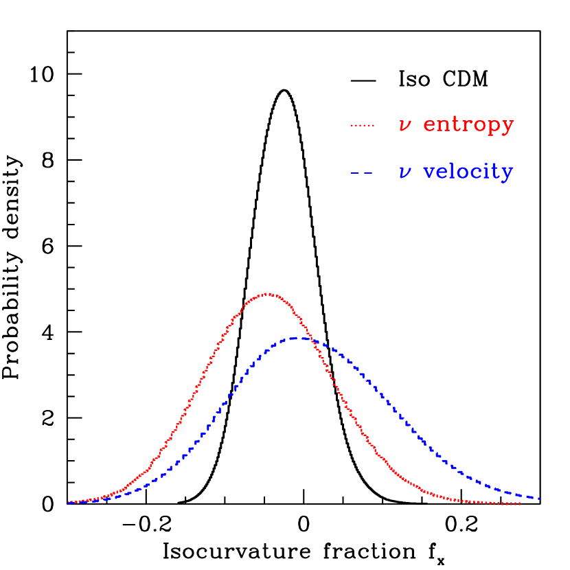
Figure 1: Normalized posterior probability density for the isocurvature fraction parameter $f_{x}$. CMB and large scale structure data are compatible with purely adiabatic initial conditions, with a slight tendency towards negatively correlated isocurvature components.

In Figure 1 we plot the 1–dimensional, marginalized posterior pdf on the isocurvature fraction parameter $f_{x}$. We we have adopted a flat prior of $f_{x}$ of width much larger than the posterior, so that the range of the prior does not influence the result. The isocurvature fraction is compatible with zero for all three isocurvature modes, with a slight shift of the peak of the pdf to negative values. This corresponds to a negative correlation, in which case the contribution to the large scales CMB power due to the isocurvature auto–correlation spectrum is largely compensated by the negative correlator. The posterior mean and standard deviation for $f_{x}$ are given in Table 1, as well as 1–dimensional marginalized intervals encompassing $95\%$ of probability. We find that the isocurvature fraction for the CDM mode is constrained to be $-0.10<f_{\text{ci}}<0.06$ ($95\%$ probability), while for the two neutrino modes we obtain $-0.20<f_{\text{ne}}<0.12$ (neutrino entropy) and $-0.18<f_{\text{nv}}<0.22$ (neutrino velocity). We notice that the tightest constrained mode is the CDM isocurvature one. This is because with our definition of $f_{x}$, for a given value of $f_{x}$ the CDM isocurvature is the mode with the largest contribution to the CMB power spectrum. Also, all of the 1–dimensional pdf’s for $f_{x}$ are very close to Gaussian. Hence we expect that Eq. (7) is a good approximation to the Bayes factor, Eq. (6), as we now show.

Table 1: Constraints on the isocurvature fraction $f_{x}$, from WMAP3 and other CMB data, and SDSS matter power spectrum measurements. We give the posterior mean $\mu$ and standard deviation $\sigma$, as well 1–dimensional marginalized regions encompassing $95\%$ of posterior probability.

Model	$\mu$	$\sigma$	95% interval on $f_{x}$
CDM iso	$-2.5\cdot 10^{-2}$	$4.0\cdot 10^{-2}$	$-0.10\dots 0.06$
$\nu$ entropy	$-4.4\cdot 10^{-2}$	$8.0\cdot 10^{-2}$	$-0.20\dots 0.12$
$\nu$ velocity	$-1.2\cdot 10^{-2}$	$1.0\cdot 10^{-1}$	$-0.18\dots 0.22$

We now evaluate the Bayes factor between the models including an isocurvature contribution and the simplest, purely adiabatic model. As we have seen above in the parameter extraction step, there is no indication that the data require and isocurvature component, since the isocurvature fraction is compatible with 0 . This is consistent with the findings of Bean et al. (2006). We therefore expect the Bayes factor to favour the purely adiabatic model on the ground of the Occam’s razor argument. The strength of evidence in favour of the adiabatic model depend on the amount of wasted parameter space for the isocurvature fraction, i.e. by the prior range $\Delta f$. In the top panel of Figure 2, we plot the Bayes factor as a function of the prior width $\Delta f$, while in the bottom panel we plot the Bayesian complexity, i.e. the number of parameters effectively constrained by the data. We can see that for models with poor predictivity, i.e. a large prior accessible range $\Delta f\gg 1$, one finds strong ($>20:1$) to decisive ($>150:1$) posterior odds against the extended model for all of the three isocurvature modes. We also plot the Gaussian approximation to the SDDR for the Bayes factor, Eq (7), for the CDM isocurvature mode, and find a very good match with the value computed numerically from the Monte Carlo chain.

For a prior choice $\Delta f\leq 1$, the Bayesian complexity is close to 7, indicating that all of the 7 parameters of the extended model have been measured. We therefore conclude that models predicting up to the same amount of isocurvature to adiabatic power (the case $\Delta f=1$) are strongly disfavoured for the CDM mode, and mildly disfavoured in the case of the two neutrino modes. However, if the prior range is reduced below $\Delta f=1$, i.e. for models predicting predominantly adiabatic initial conditions with subdominant isocurvature contribution, the Bayes factor gives an inconclusive result, with about equal odds for the purely adiabatic and the mixed models. At the same time, the Bayesian complexity decreases, indicating that $f_{x}$ is only poorly constrained with respect to the scale of the prior, especially for the neutrino density and velocity modes. This reinforces the conclusion that current data are not strong enough to select among a purely adiabatic model and one which predicts up to $10\%$ isocurvature contribution and we need to acquire better data in order to obtain a higher–odds result.

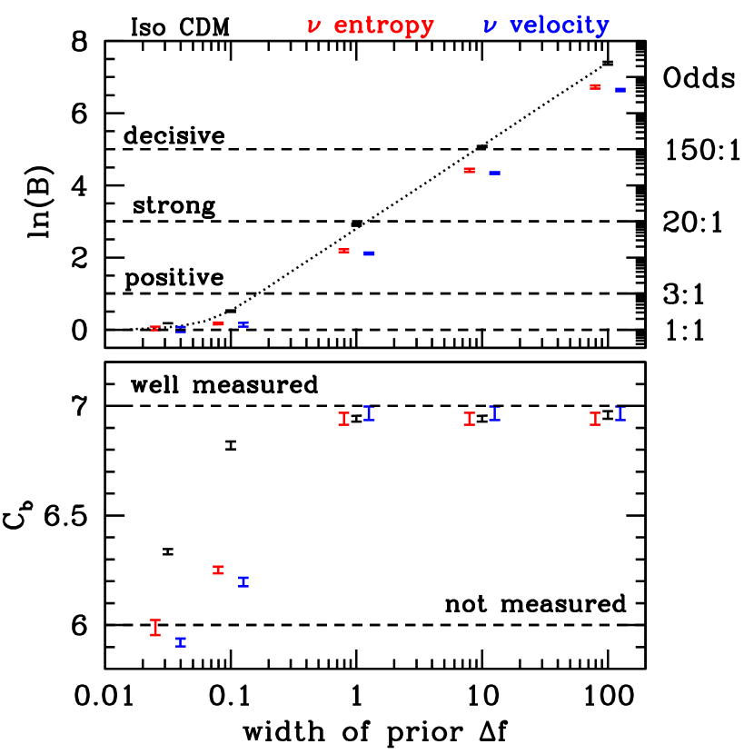
Figure 2: Result of model selection between a purely adiabatic model and an extended model featuring a totally (anti–)correlated isocurvature component, as a function of the prior available range for the isocurvature fraction, $\Delta f$. Top panel: the Bayes factor strongly disfavours models with $\Delta f\gg 1$ because of the Occam’s razor effect, while models predicting an isocurvature fraction below about $10\%$ in any of the three modes cannot presently be ruled out ($\ln B<1$). The dotted line gives the Gaussian approximation to the Bayes factor, Eq. (7), for the CDM isocurvature mode. Bottom panel: the Bayesian complexity gives the effective number of parameters the data can support. For $\Delta f\,\raise 1.72218pt\hbox{$<$}\kern-8.00003pt\lower 2.6694pt\hbox{$\sim$}\,1$ the isocurvature component in the neutrino entropy and velocity modes is not supported by the data. The errors have been computed as the variance of 10 random sub–chains, and the neutrino entropy and velocity modes have been shifted horizontally to the left and to the right, respectively, for clarity.

5 Conclusions

We have submitted the question of the type of initial conditions for cosmological perturbations to renewed scrutiny in the light of WMAP 3–year data. We have focused on the simplest and well motivated alternative to a purely adiabatic model, namely an admixture of one totally (anti–)correlated isocurvature mode at the time, with the same spectral tilt as the adiabatic one.

We have derived posterior bounds on the isocurvature fraction from WMAP 3–year data combined with other CMB measurements and SDSS. We have constrained the isocurvature fraction in the CDM mode to be less than about $10\%$, while the maximum allowed neutrino isocurvature contribution (either density or velocity) is about $20\%$.

Bayesian model selection tends to favour purely adiabatic initial conditions with strong odds ($>20:1$) when compared to models predicting isocurvature fractions larger than unity. For such models – having a large prior range on the isocurvature fraction – we have shown that the data can support 7 parameters, but that only 6 of them are required, with no need to include isocurvature modes from a model selection point of view. These findings confirm the conclusions of Kunz et al. (2006). However, mixed models that limit the isocurvature contribution to less than about $10\%$ cannot presently be ruled out. We have shown that the constraining power of the data for this class of models is insufficient, and therefore we must hold our judgement until better data becomes available. These findings are however dependent on the parameterization chosen for the isocurvature fraction, that in this work is motivated by the curvaton scenario. The question of prior selection will be further addressed in a future publication.

It is reasonable to expect that the same conclusion would apply in even stronger terms to the case of more complicated models, e.g. those involving a superposition of different isocurvature modes at the same time, or with arbitrary correlations among them. In fact, more complicated models (such as the class considered by Bean et al. (2006)) ought to be even more disfavoured because of their larger volume of wasted parameter space. At present, Occam’s razor is perfectly compatible with the simplest possibility, namely purely adiabatic initial conditions.

We think that this model comparison approach can be a useful complement to parameter constraints analysis, and that it can offer valuable guidance in building models for the generation of primordial perturbations.

Acknowledgments R.T. is supported by the Royal Astronomical Society through the Sir Norman Lockyer Fellowship. I am grateful to Andrew Liddle and David Parkinson for comments. I acknowledge the use of the package cosmomc, available from cosmologist.info and the use of the Legacy Archive for Microwave Background Data Analysis (LAMBDA). Support for LAMBDA is provided by the NASA Office of Space Science.

References

- Bean et al. (2006) Bean R., Dunkley J., Pierpaoli E., 2006, astro-ph/0606685
- Beltran et al. (2005) Beltran M., Garcia-Bellido J., Lesgourgues J., Liddle A. R., Slosar A., 2005, Phys. Rev., D71, 063532
- Beltran et al. (2004) Beltran M., Garcia-Bellido J., Lesgourgues J., Riazuelo A., 2004, Phys. Rev., D70, 103530
- Beltran et al. (2005) Beltran M., Garcia-Bellido J., Lesgourgues J., Viel M., 2005, Phys. Rev., D72, 103515
- Bucher et al. (2000) Bucher M., Moodley K., Turok N., 2000, Phys. Rev., D62, 083508
- Bucher et al. (2001) Bucher M., Moodley K., Turok N., 2001, Phys. Rev. Lett., 87, 191301
- Durrer (2004) Durrer R., 2004, Lect. Notes Phys., 653, 31
- Freedman et al. (2001) Freedman W. L., et al., 2001, Astrophys. J., 553, 47
- Gordon & Lewis (2003) Gordon C., Lewis A., 2003, Phys. Rev., D67, 123513
- Hinshaw et al. (2006) Hinshaw G., et al., 2006, astro-ph/0603451
- Kass & Raftery (1995) Kass R., Raftery A., 1995, J. Amer. Stat. Assoc., 90, 773
- Kunz et al. (2006) Kunz M., Trotta R., Parkinson D., 2006, Phys. Rev. D 74, 023503
- Kuo et al. (2004) Kuo C.-l., et al., 2004, Astrophys. J., 600, 32
- Lyth & Wands (2002) Lyth D. H., Wands D., 2002, Phys. Lett., B524, 5
- Moodley et al. (2004) Moodley K., Bucher M., Dunkley J., Ferreira P. G., Skordis C., 2004, Phys. Rev., D70, 103520
- Page et al. (2006) Page L., et al., 2006, astro-ph/0603450
- Readhead et al. (2004) Readhead A. C. S., et al., 2004, Astrophys. J., 609, 498
- Tegmark et al. (2004) Tegmark M., et al., 2004, Astrophys. J., 606, 702
- Trotta (2004) Trotta R., 2004, PhD thesis, University of Geneva, Thesis N. 3534, astro-ph/0410115
- Trotta (2005) Trotta R., 2005, astro-ph/0504022
- Trotta & Durrer (2004) Trotta R., Durrer R., 2004, Proceedings of the MG10 Meeting, Rio de Janeiro, Brazil 20–26 July 2003 (M. Novello and S. Perez Bergliaffa, Eds) World Scientific, astro-ph/0402032
- Trotta et al. (2001) Trotta R., Riazuelo A., Durrer R., 2001, Phys. Rev. Lett., 87, 231301
- Trotta et al. (2003) Trotta R., Riazuelo A., Durrer R., 2003, Phys. Rev., D67, 063520
- Trotta (2006) Trotta R., To appear in Proceedings of the Conference on Cosmology, Galaxy Formation and Astro-Particle Physics on the Pathway to the SKA, Oxford, England, 10–12 Apr 2006. arXiv:astro-ph/0607496.