Anomalous H₂CO Absorption Towards the Galactic Anticenter:
A Blind Search for Dense Molecular Clouds

Abstract

We have carried out a blind search in the general direction of the Galactic Anticenter for absorption of the Cosmic Microwave Background (CMB) radiation near 4.83 GHz by molecular clouds containing gaseous ortho-formaldehyde (H₂CO). The observations were done using the 25-m radio telescope at Onsala in Sweden, and covered strips in Galactic latitude $-1^{\circ}\leq b\leq+1^{\circ}$ at several longitudes in the region $170^{\circ}\leq l\leq 190^{\circ}$. Spectra were obtained in these strips with a grid spacing corresponding to the telescope resolution of $10^{\prime}$. We have detected H₂CO CMB absorption at $\approx 10\%$ of the survey pointings. This detection rate is likely to increase with further improvements in sensitivity, and may become comparable to the detection rate expected from a blind CO survey with a corresponding sensitivity limit. We have mapped some of these detections in more detail and compared the H₂CO absorption to existing maps of CO(1-0) emission in the same regions. There appears to be a rough correlation between the velocity-integrated line strength of the CO(1-0) emission and that of the H₂CO absorption. However, the scatter in this correlation is significantly larger than the measurement errors, indicating differences of detail at and below the linear resolution of our observations ($\approx 4-9$ pc). Although these two tracers are expected to have similar excitation requirements on the microscopic level characteristic of warm, T${}_{K}>10$K, dense, $10^{3}<n<10^{5}$ cm^-3 condensations in molecular clouds, the CO(1-0) line is expected to be optically thick, whereas the H₂CO line is not. This latter difference is likely to be responsible for a significant part of the scatter in the correlation we have found.

1 Introduction

Following on the discovery of the anomalous absorption of the Cosmic Microwave Background (CMB) at 4.83 GHz by gas-phase ortho-formaldehyde (H₂CO) molecules in a few nearby Galactic dark nebula (Palmer et al., 1969), several surveys were carried out in hopes of establishing the general Galactic distribution of distant dusty molecular clouds containing gaseous H₂CO. Gordon & Roberts (1971) used the NRAO 140-foot telescope (beam FWHM $\approx 6^{\prime}$, system temperature T${}_{S}\approx 85$ K) to survey 30 positions spread out along the Galactic plane near $b=0^{\circ}$ in the range $2.0^{\circ}\leq l\leq 251.1^{\circ}$ and chosen to be free of radio continuum emission. With the exception of the one position near to the Galactic center (which did indeed appear to have continuum emission in the general area), no detections of CMB absorption could be registered, with a typical peak limits (5$\sigma$) of 0.07 K in a velocity channel of width 1.6 km s^-1. Gordon & Roberts concluded either that the excitation temperature of the general Galactic distribution of H₂CO must be close to the brightness temperature of the CMB (now known to be 2.73 K), or that the dust clouds harboring the H₂CO must be much smaller than the telescope beam. This disappointing result was corroborated with additional observations by Gordon & Höglund (1973) using the 25-m radio telescope of the Onsala Space Observatory (OSO) in Sweden (FWHM $\approx 10.5^{\prime}$, T${}_{S}\leq 55$ K) in order to map three $1^{\circ}\times 1^{\circ}$ fields in the Galactic plane at $l=48^{\circ},70^{\circ}$, and $110^{\circ}$. Spectra were obtained in each of these fields on a grid with separation $10^{\prime}$. No emission or absorption was found, with a typical peak limit of 0.15 K in a 0.62 km s^-1 channel.

The first large-scale survey for H₂CO along the Galactic plane was carried out by Few (1979) using the Jodrell Bank Mark II radio telescope (FWHM $9.6^{\prime}\times 10.3^{\prime}$, T${}_{S}\approx 70$ K). Observations were made at $b=0^{\circ}$ every $2^{\circ}$ of Galactic longitude in the range $8^{\circ}\leq l\leq 60^{\circ}$ and every $1^{\circ}$ in the range $14^{\circ}\leq l\leq 36^{\circ}$. These observations were successful in recording H₂CO absorption in the inner Galaxy, and some approximate information on the spatial distribution was obtained. However, the signal dropped to undetectable levels beyond $l\gtrsim 50^{\circ}$, and no observations were attempted in the outer Galaxy. In fact, at no position did the absorption-line profile depth exceed the observed continuum temperature. One can therefore safely conclude that what was being measured was not the anomalous CMB absorption (which was still apparently too weak), but rather absorption of the Galactic background radio radiation, which is strongest in the inner Galaxy.

Although gaseous H₂CO may be nearly absent in parts of the ISM because it is dissociated or frozen out on grains, these early surveys provided an indication that the physical conditions under which detectable anomalous H₂CO absorption occurs may not be common in the Galaxy. Observers turned their attention to other, more easily detected molecules, notably CO, and we now have extensive surveys of the CO(1-0) line over large sections of the Galactic plane (Dame et al., 1987; Combes, 1991; Dame et al., 2001). These surveys, along with many detailed studies of specific molecular clouds in a wide range of molecular tracers, have all contributed to a much more complete (and much more complicated) view of physical conditions in the cool molecular ISM.

An explanation for the anomalous CMB absorption by H₂CO was first suggested by Townes & Cheung (1969) using a classical calculation for collisional excitation. Subsequent work, especially by Evans and his collaborators (Evans, 1975; Evans et al., 1975), confirmed this result using quantum mechanical calculations and observations. The collisional pumping mechanism is more effective at high collision rates, so in general the absorption is strongest at higher densities and temperatures. However, the calculations by Evans (1975) showed that the mechanism would still be effective at rather low temperatures, below about 10K. More precise quantum mechanical calculations reported by Garrison et al. (1975) suggested a smaller effect at very low kinetic temperatures, but both methods involved approximations. This leaves open the possibility that high-density, cold clumps of molecular gas in the ISM may be detectable in H₂CO absorption, and has provided part of the motivation for our observing program.

Our approach is to carry out long integrations at a set of blindly-selected positions in the general direction of the Galactic Anticenter. For these observations we have again used the 25-m OSO radio telescope at Onsala, the same telescope used by Gordon & Höglund more than 33 years ago in their failed attempt to detect the general H₂CO CMB absorption. Our present success is due entirely to the availability of more sensitive receivers and to generous allocations of observing time on this telescope. Our survey has two main features: First, it is a “blind” survey; we purposely avoided using maps of any other ISM tracer to construct the observing program. Second, we chose to observe in the Galactic anticenter region, i.e. in the general direction of the outer Galaxy. The Galactic nonthermal background at 6 cm is exceedingly faint in this direction, so we can be fairly confident that any absorption we might detect is indeed anomalous CMB absorption. We will return to this point later. Also, the velocity gradient owing to Galactic rotation is small in the anticenter direction, so we might hope for some degree of “bunching” of absorption features, enhancing the probability of detection.

2 Observations and results

The observations were obtained during two sessions, the first in September-October 2004, and the second in May 2005, with the 25m Onsala radio telescope. At 6 cm, the angular resolution of the telescope is FWHM $\approx 10^{\prime}$, and the pointing precision is better than $20^{\prime\prime}$. The local oscillator was operated in frequency-switching mode with a “throw” of 0.8 MHz, and both (circular) polarizations of the incoming signal were recorded simultaneously in two independent units of a digital autocorrelator spectrometer. Each of these units provided 800 channels spaced by 4 kHz. At the frequency of the 1₁₁-1₁₀ line of ortho-H₂CO (4829.660 MHz), this setup provided a total bandwidth of 3.2 MHz = 199 km s^-1 and a (twice-hanning-smoothed) velocity resolution of 16 kHz = 0.99 km s^-1. Daily observations of Cas A were made in order to check the overall performance of the receiver. The system temperature during our sessions varied from 33 to 36 K. The off-line data reduction was done with the CLASS/GILDAS software system (Guilloteau & Forveille, 1989), and involved only the subtraction of (flat) baselines from individual integrations and the averaging of all spectra taken at the same pointing position. The total integration time at each pointing position was $\approx 2$ hours, yielding a final typical rms noise level of 0.0035 K (T${}^{*}_{A}$) and a 5$\sigma$ detection limit of 0.0175 K in each $\approx 1$ km s^-1 channel.

2.1 The blind search

For our blind search, integrations were made every $10^{\prime}$ in 11 strips perpendicular to the Galactic plane from $-1^{\circ}$ to $+1^{\circ}$ at intervals of $2^{\circ}$ in Galactic longitude from $170^{\circ}$ to $190^{\circ}$. The spectrometer was centered at a slightly different systemic velocity for each strip (cf. Table 1), following the expected run of radial velocity according to the “standard” model of rotation in the outer Galaxy using HI data from Hartmann & Burton (1997).

Table 1: Spectrometer systemic velocity used at each longitude

Longitude (deg.)	170	172	174	176	178	180	182	184	186	188	190
Velocity (km s-1)	-12	-9.7	-8.5	-7.3	-5.4	-3.1	-1.0	1.4	3.1	4.3	6.2

The final (averaged) spectra are shown as a mosaic in Figure 1. There is clear evidence for absorption in 10 – 12 positions, and hints of absorption in several more. It is evident that, with our increased level of sensitivity, we have successfully detected H₂CO absorption at roughly 10% of the total of 143 positions observed. It is also interesting to note that we have not recorded any H₂CO emission; this may indicate that very dense gas with $n\gtrsim 10^{5}$ (see §4) is rare, with a low area filling factor, and/or the gas is much colder than about 10 K. For reference, Figure 1 also shows the disposition of our survey positions with respect to the CO emission obtained from the survey by Dame et al. (2001). We will return to this comparison later, but we wish to emphasize here that our choice of H₂CO survey positions took no prior account of the distribution of CO emission. Nevertheless, it is clear from this Figure that the H₂CO absorption is seen most strongly in regions of strong CO emission. Figure 1 also shows regions of faint CO emission without corresponding H₂CO absorption; for instance several survey points at $l=188^{\circ}$ are located in a region of faint CO emission. The absence of H₂CO absorption at such positions is likely to be a reflection of the sensitivity limit of our observations.

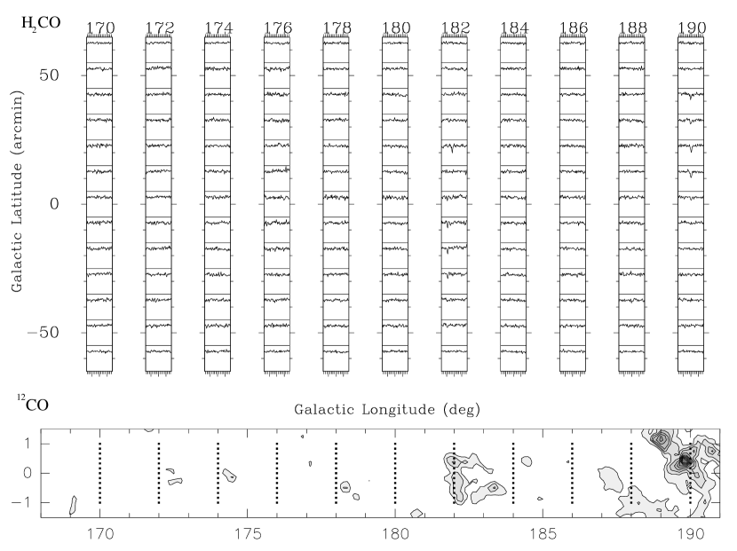
Figure 1: Mosaic of H₂CO spectra at 143 positions towards the Galactic anticenter. The Galactic longitude of each strip is given at the top of the figure, and the Galactic latitude on the left side. The velocity scale along the bottom of each longitude strip is centered at the values given in Table 1; the short tick marks indicate increments of 1 km s^-1 and the longer ticks are at intervals of 5 km s^-1. The lower panel shows the survey positions superposed on a map of the CO emission in the area, see text for details.

2.2 Mapping observations

The presence of two regions of relatively strong absorption can be identified in Figure 1, the first at $l\approx 182^{\circ}$, and the second at $l\approx 190^{\circ}$. We have mapped these two regions in more detail in order to examine the distribution of H₂CO absorption and to permit a point-by-point comparison with the existing CO(1-0) emission surveys in this region of the Galaxy. The receiver settings for these two maps were identical to those used for the blind survey, and the total integration times per pointing position were similarly long.

Figure 2a (left panel) shows profiles at 63 of 66 positions on a grid centered (position 0,0) at $l=182^{\circ}$, $b=0^{\circ}$, with an interval of $10^{\prime}$. Similarly, Figure 3a (left panel) shows profiles at 101 of 121 positions on a grid centered (position 0,0) at $l=190^{\circ}$, $b=0^{\circ}$, also with an interval of $10^{\prime}$.

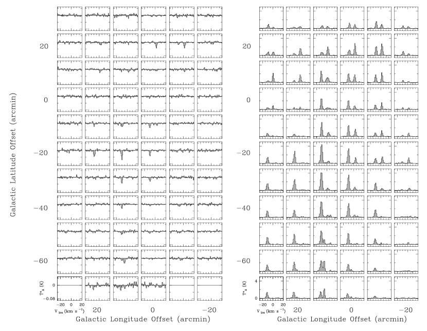
Figure 2: a.(left panel) Mosaic of H₂CO spectra observed in the direction $l=182^{\circ}$, $b=0^{\circ}$. b.(right panel) Observations of CO(1-0) at corresponding positions, from the Columbia survey, smoothed to $10^{\prime}$ (see text).

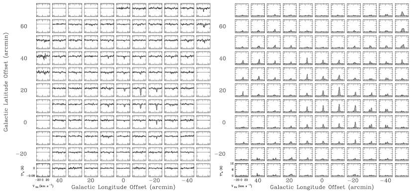
Figure 3: a.(left panel) Mosaic of H₂CO spectra observed in the direction $l=190^{\circ}$, $b=0^{\circ}$. b.(right panel) Observations of CO(1-0) at corresponding positions, from the Columbia survey, smoothed to $10^{\prime}$ (see text).

3 Analysis

3.1 The nature of the H₂CO absorption

How can we be sure that the absorption we have recorded, both in our blind search and in our two detailed maps, is actually absorption of the CMB? We have earlier argued that it is not likely to be absorption of the Galactic nonthermal background, since this background is very faint in the outer Galaxy at 6 cm, so we can confidently rule out the type of absorption recorded in the inner Galaxy by Few (1979). But what about discrete continuum sources in the background, perhaps distant H ii regions or radio galaxies? In order to examine this possibility, we have retrieved radio continuum survey data at 21-cm from Reich et al. (1997) covering the two regions we have mapped in detail. Figure 4 shows the 21-cm continuum in these two regions observed with the Effelsberg 100-m telescope at a resolution of $9.4^{\prime}$ (contours) overlaid on our H₂CO absorption data (grey scale, resolution $\approx 10^{\prime}$). From the general lack of correspondence of the radio continuum peaks with the H₂CO absorption maxima we can safely conclude that it is indeed the CMB absorption we have recorded in H₂CO. Furthermore, the continuum sources are either behind the H₂CO absorbers, or the area filling factor of the absorbing clouds is small and the line of sight to the sources just misses the clouds.

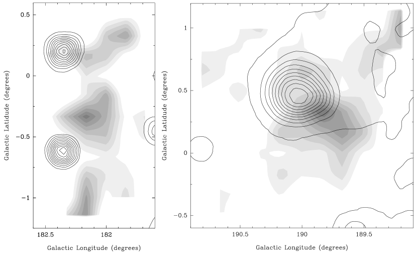
Figure 4: The location of the 21-cm radio continuum emission (contours, Effelsberg 100-m telescope, FWHM $9.4^{\prime}$) overlaid on our H₂CO observations (grey scale, Onsala 25-m telescope, FWHM $\approx 10^{\prime}$). a.(left panel) detailed survey area near $l=182^{\circ}$, $b=0^{\circ}$. b.(right panel) detailed survey area near $l=190^{\circ}$, $b=0^{\circ}$.

3.2 Statistics of the H₂CO absorption

Our blind search has succeeded in recording anomalous H₂CO absorption at approximately 10% of the survey positions. This is a significant improvement over the earlier blind searches of Gordon & Roberts (1971) and Gordon & Höglund (1973), which failed to record any such absorption. Since we have no reason to believe that the regions chosen for the early searches are in any way peculiar, we conclude that our success is likely due to the large improvement in sensitivity of our observations. Our rms noise level is typically 0.0035 K (T${}^{*}_{A}$) for a 5$\sigma$ detection limit of 0.0175 K. When compared at the same velocity resolution, this is an improvement of $\approx 5$ over the observations of Gordon & Roberts (1971) and a factor $\approx 6.8$ over those of Gordon & Höglund (1973). This result strongly suggests that the detection rate is simply sensitivity limited, and that it would increase with further increases in sensitivity. Future searches would benefit from using larger telescope apertures with more collecting area; beam dilution would also be reduced on the more distant dust clouds.

3.3 Relation of H₂CO CMB absorption to CO(1-0) emission

We have retrieved the CO(1-0) emission line data for our two mapped fields from the survey by Dame et al. (2001), smoothed that data slightly from its original $8.4^{\prime}$ resolution to the $10^{\prime}$ resolution of our H₂CO observations, and extracted profiles at the same positions as on our maps near $l=182^{\circ}$, $b=0^{\circ}$ and $l=190^{\circ}$, $b=0^{\circ}$. The results are shown in the right panels of Figure 2 and Figure 3. A cursory inspection of these mosaics shows that there is an overall general correlation between the two tracers, in particular, at every position where we have detected H₂CO, CO(1-0) emission is also detected. The converse is not always true; there are many positions where CO(1-0) is easily detected which show no corresponding H₂CO above the noise. Although this may simply be a consequence of a lower S/N for the H₂CO observations, a more detailed look at these profiles reveals that S/N is not the whole story. In particular, the H₂CO absorption profiles are not merely scaled versions of the CO(1-0) emission profiles. Consider the profiles on the mosaic of Figure 3 at $l=190^{\circ}$, in particular those at (-20,+10), (-10,+10), and (0,+10). In H₂CO this sequence of 3 profiles shows a uniform decrease in the depth of the absorption from about -0.05 to -0.04 to -0.03 K, but in CO the emission profiles peak at about 6, 7, and 6 K respectively.

Another way of showing the general correlation between CO and H₂CO is depicted in Figures 5 and 6, which show contour maps of the two components in a latitude-velocity plot integrated over a small range in longitude. Figure 5 shows the two velocity components in this region, a weaker component at $\approx+2.5$ km s^-1, and a stronger component at $\approx-10$ km s^-1. Figure 6 shows the data for the region centered at $l=190^{\circ}$ in the same latitude-velocity presentation. The principal component here is observed at $\approx+8.5$ km s^-1. These figures confirm the general similarity of the CO emission and the H₂CO absorption. The H₂CO CMB absorption clearly generally traces the same molecular gas seen in the more ubiquitous (and easier to observe) CO molecule.

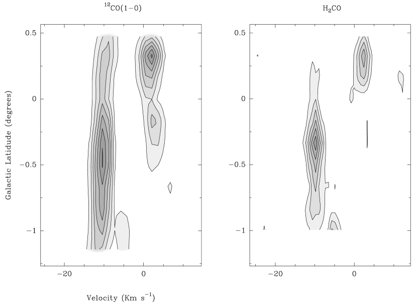
Figure 5: a.(left panel) Latitude-velocity contour maps of ¹²CO emission and b.(right panel) H₂CO absorption observed in the direction $l=182^{\circ}$, $b=0^{\circ}$. The data have been integrated over the longitude range from $l=181.7^{\circ}$ to $l=182.5^{\circ}$ in both panels.

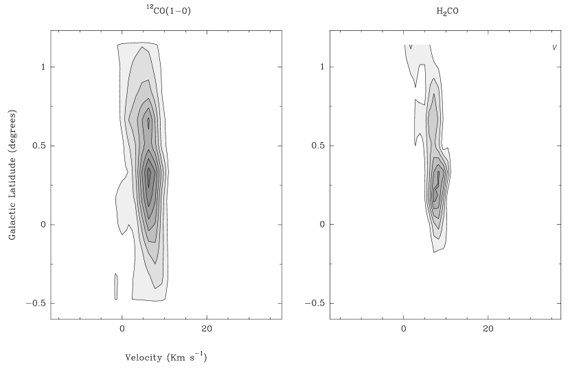
Figure 6: a.(left panel) Latitude-velocity contour maps of ¹²CO emission and b.(right panel) H₂CO absorption observed in the direction $l=190^{\circ}$, $b=0^{\circ}$. The data have been integrated over the longitude range from $l=189.2^{\circ}$ to $l=190.8^{\circ}$ in both panels.

A general correspondence of H₂CO and ¹²CO(1-0) was also noted by Cohen et al. (1983) in their extensive mapping study of H₂CO and OH in the Orion region. Those authors found a broad general agreement in that well-known star-forming region, but concluded that the detailed agreement was poor. They found a better correspondence with ¹³CO(1-0), and concluded that the reason for this was that the optically-thick ¹²CO(1-0) line was primarily tracing gas temperature, whereas the ¹³CO(1-0) emission and the H₂CO absorption are both optically-thin lines that will trace primarily the density. In general we agree with this interpretation, although as we will discuss in more detail later the dependence of the H₂CO absorption on kinetic temperature is also likely to be playing a role.

In order to study the relation between H₂CO absorption and CO(1-0) emission in more detail, we have computed the moments of the profiles shown in Figures 2 and 3. The results are listed in Tables 3 and 4 (see the electronic version of this paper). If two components are visible at a given pointing, the moments for each have been computed separately; in many cases a second component was too weak to be identified in H₂CO. Components that exceed the $3\sigma$ limit are indicated in column 6 of these tables and their values plotted in the correlation diagram of Figure 7. Since the data in the two fields did not seem to show any different trends, we have included the profile intensities from both fields in Figure 7.

Figure 7: The correlation between the H₂CO absorption line intensity and the CO(1-0) emission line intensity at corresponding points in the two fields surveyed in detail. The triangles correspond to data from Table 3, the squares to data from Table 4, and the open circles correspond to H₂CO upper limits (points where the CO was detected but H₂CO was not). The horizontal and vertical lines show the $\approx 3\sigma$ noise for the spectra with the lowest noise. The least squares fitted line is shown dashed. The data tables are shown in the electronic version of this paper.

We have fitted the data in Figure 7 by least squares to a straight line; the result is:

$$I(H_{2}CO)=a\times I(CO)+b$$ (1)

yielding a value of $a=-0.0041\pm 0.0005$ and $b=-0.034\pm 0.013$. While the fit is not bad, in several cases the data points lie significantly off the best-fit line. We will return to this point in the Discussion below.

3.4 Other sources in the two mapped fields

In order to have some idea of the distances to our detections, we have searched the Catalog of Star-Forming Regions in the Galaxy (Avedisova, 2002) for objects at known distances which may be associated with them. Table 3.4 lists several IRAS sources which are candidates, and their associated distances. These distances were obtained from the references listed in the table, and were determined from optical (H ii regions) and radio spectroscopy (CO(1-0) in molecular clouds) and using a model rotation curve of the outer Galaxy.

Table 2: IRAS sources possibly associated with CO and H₂CO emission in Figures 8 and 9.

IRAS source	Position (l,b)	Associated object	Distance (kpc)	References
IRAS 05490+2658	182.4, +0.3	S242	2.0 - 2.1	1, 2
IRAS 05431+2629	182.1, -1.1		0.1 *	3
IRAS 06067+2138	189.1, +1.1		0.9 *	3
IRAS 06051+2041	189.7, +0.3		2.3 *	3
IRAS 06055+2039	189.8, +0.3	Gem OB1, S252	1.5 - 2.9 *	3, 4, 5
IRAS 06063+2040	189.9, +0.5	Gem OB1, AFGL5183	1.5 - 2.8 *	3, 4, 6
IRAS 06068+2030	190.1, +0.5	S252, AFGL5184	1.5 - 2.7 *	1, 3, 6, 7
IRAS 06061+2028	190.0, +0.3		2.3 *	3
IRAS 06079+2007	190.5, +0.6		2.6 *	3

Note. — In all the cases the distances are taken from the published literature.

These distances are determined from spectroscopy of the exciting stars of the associated H ii regions.

** Kinematic distances using ¹²CO data and a model rotation curve of the outer Galaxy.

References. — (1) Blitz et al. (1982), (2) Carpenter et al. (1995), (3) Wouterloot & Brand (1989), (4) Humphreys (1978), (5) Snell et al. (1990), (6) Snell at al. (1988), (7) Moffat et al. (1979).

In Figures 8 and 9 we show contour plots of the H₂CO and CO profile fluxes integrated over velocity for our two detailed fields. The IRAS sources from Table 3.4 are indicated with the black triangles. We conclude that the correspondence is only marginal, but the results suggest that the regions we have found are likely to be located at distances of 1.5 - 3 kpc, probably in the Perseus arm of the Galaxy (2 – 3 kpc from the sun). In that case our $10^{\prime}$ beam corresponds to a linear resolution of 4 - 9 pc.

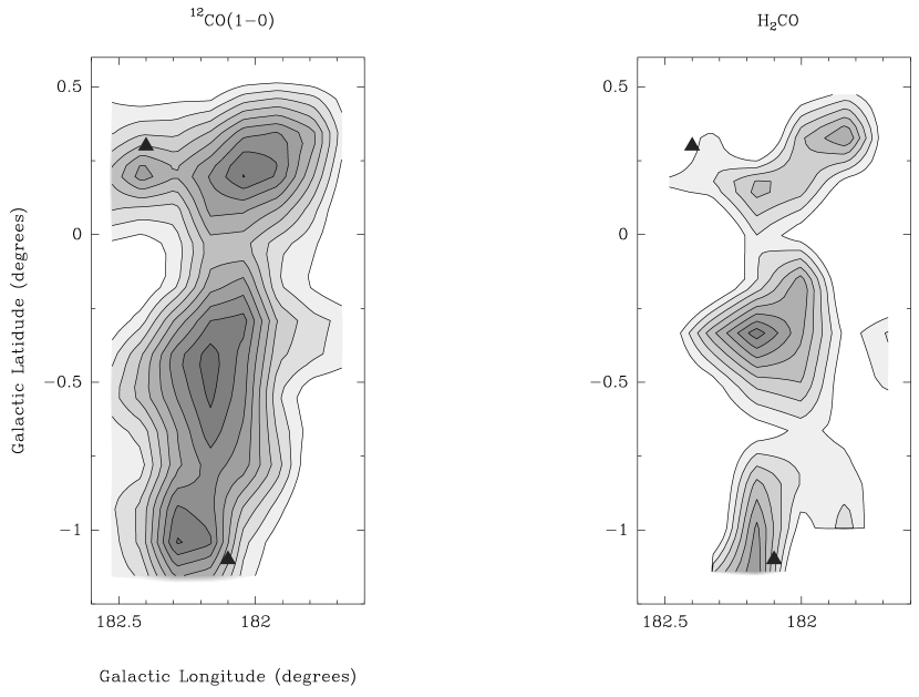
Figure 8: a.(left panel) Velocity-integrated contour map of the ¹²CO emission for the first region mapped in the direction $l=182^{\circ}$, $b=0^{\circ}$. b.(right panel) Velocity- integrated H₂CO absorption for the same region. The blue triangles show the positions of IRAS sources possibly associated with features in these regions. The velocity range extends from -16.0 km s^-1 to 6.0 km s^-1 in both panels.

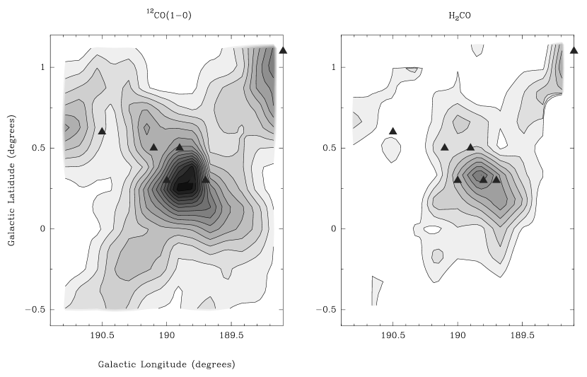
Figure 9: a.(left panel) Velocity-integrated contour map of the ¹²CO emission for the second region mapped in the direction $l=190^{\circ}$, $b=0^{\circ}$. b.(right panel) Velocity- integrated H₂CO absorption for the same region. The blue triangles show the positions of IRAS sources possibly associated with features in these regions. The velocity range extends from -3.0 km s^-1 to 16.0 km s^-1 in both panels.

4 Discussion

The general correlation between the integrated line intensities of the CO(1-0) emission and the H₂CO absorption suggests that the excitation characteristics of these two lines are similar. In fact, both of these lines trace warm, dense molecular gas, as various calculations have shown in many historical papers. For instance, Helfer & Blitz (1997) show examples of emergent brightness calculations for CO(1-0) in the Galactic GMC Lynds 1204 in the context of one popular model (the large-velocity-gradient model). As their Figure 1 shows, the observed brightness of this (usually optically-thick) line is essentially proportional to the kinetic temperature of the gas as long as the density exceeds the critical density of $\approx 10^{3}$ ${\rm cm^{-3}}$. It follows that any sensitivity-limited CO(1-0) survey will therefore preferentially record the warm, dense regions of the ISM.

The details of H₂CO 6-cm line formation have been studied for example in several papers by Evans and co-workers (Mundy et al. (1987); Young et al. (2004)). The 6 cm absorption line arises through collisions to higher rotational levels followed by radiative decay to the ground level, which becomes overpopulated owing to small differences in collision cross sections. The line is therefore generally stronger if the collision rate is higher, so this too favors warm, dense clouds. However, the absorption line is quenched at very high collision rates, when the level populations approach a Boltzmann distribution, and the 6 cm line then goes into emission. In a future paper on H₂CO mapping of the large Galactic dust cloud Lynds 1204 (Rodriguez et al., 2006) we will present model computations of H₂CO absorption in more detail. For the moment we note that the 6 cm absorption is strongest in the density range of $10^{3}\lesssim n\lesssim 10^{5}$ ${\rm cm^{-3}}$. In our model the absorption is deepest at $n\approx 10^{4.3}$ ${\rm cm^{-3}}$, first appearing at $T_{K}\gtrsim 10$ K, and saturating at $T_{K}\approx 40$ K in the sense that the absorption hardly increases for higher temperatures. This dependence on kinetic temperature is therefore somewhat different than is the case for the CO(1-0) line; this is mostly a consequence of the fact that the H₂CO line remains optically thin, so it more closely reflects the specific excitation conditions.

One of the premises for doing the blind search for H₂CO towards the Galactic Anticenter was the possibility of finding molecular gas in regions where CO emission had not previously been detected. This could potentially reveal a component of the molecular gas characterized by an excitation temperature lower than that corresponding to the energy level of the first rotational transition of CO (or any other commonly observed molecule). Such an excitationally cold molecular gas component would only be observable in absorption, either against a continuum background source or, when using the anomalous absorption of H₂CO, against the CMB. The fact that we do not see H₂CO absorption outside the regions where CO emission is observed, suggests that either such cold molecular gas is not present, or, as we will argue, the anomalous H₂CO absorption is not sensitive to excitationally cold molecular gas.

As shown by Townes & Cheung (1969) and Evans et al. (1975), the anomalous H₂CO absorption is due to collisional pumping and most effective at densities between $n_{\mathrm{H_{2}}}\approx 10^{3}-10^{5}$ cm^-3. Our observations of the 6-cm H₂CO line therefore seem to exclude the existence of dense molecular gas outside the regions probed by CO emission. However, the effectiveness of the collisional pumping at low temperatures has not been decisively determined (cf. Evans 1975; Garrison et al. 1975), and we cannot exclude the possibility of very cold molecular gas outside the CO emission regions, even if it meets the density requirement for inversion. In Rodriguez et al. (2006) we found that the effectiveness of the collisional pumping leading to the anomalous excitation of the 6-cm H₂CO transition is indeed temperature dependent, requiring a relatively high temperature. The combined requirement of a high temperature and density in order to render the anomalous H₂CO absorption line observable means that whenever present, the H₂CO absorption and CO emission lines will be spatially co-existing. Hence, the 6-cm H₂CO absorption seen against the CMB is not a viable tracer of cold molecular gas. This is discussed in more detail in Rodriguez et al. (2006).

5 Conclusions

• We have successfully detected anomalous CMB absorption by H₂CO-bearing dust clouds at $\approx 10\%$ of our blind survey positions in the direction of the outer Galaxy. No emission profiles were found.

• Our success is likely due to the large improvement in sensitivity of our observations over that of earlier surveys. This strongly indicates that the detection statistics will improve further if even higher-sensitivity searches are carried out. Since the absorption signal strength from more distant clouds will suffer from increasing beam dilution, future searches ought to be done with larger radio telescopes.

• H₂CO absorption and CO emission lines are spatially co-existing. All observed H₂CO absorption features were associated with know CO emission.

• We have found a rough correspondence between the H₂CO and the ¹²CO(1-0) line fluxes in detailed maps of two regions in our survey area. We have argued that both lines generally trace warm, dense gas in the ISM, with the situation for CO(1-0) being somewhat simpler owing to the fact that this line is usually optically thick.

Table 3: Profile moments for each position of Fig. 2. The upper limits correspond to $3\sigma$. An ellipsis …indicates no data were available; dashes — indicate data were available but no reliable fit could be made. Values marked with Y in column 6 are plotted in Figure 7.

Offset (l,b)	$100\times$ I(H2CO)	$\langle V\rangle$	I(CO)	$\langle V\rangle$	Include in
arcmin	K km s-1	km s-1	K km s-1	km s-1	Fig. 7 ?
30, -70	…	…	6.0 $\pm$ 1.7	-9.6 $\pm$ 2.8
20, -70	$<$ -9.3	—	7.2 $\pm$ 1.7	-10.6 $\pm$ 2.7
10, -70	$<$ -14.0	—	6.4 $\pm$ 0.8	-11.9 $\pm$ 1.8
	—	—	6.7 $\pm$ 1.3	-4.5 $\pm$ 1.0
0, -70	$<$ -14.0	—	4.5 $\pm$ 0.8	-11.9 $\pm$ 2.6
	—	—	$<$ 3.9	—
-10, -70	…	…	$<$ 5.7	—
-20, -70	…	…	$<$ 6.0	—
30, -60	$<$ -5.7	—	$<6.9$	—
20, -60	$<$ -6.9	—	10.0 $\pm$ 1.6	-9.3 $\pm$ 1.6
10, -60	-6.7 $\pm$ 1.9	-5.7 $\pm$ 3.2	7.3 $\pm$ 1.3	-4.2 $\pm$ 0.8	Y
	-4.5 $\pm$ 1.2	-10.3 $\pm$ 3.3	12.2 $\pm$ 0.9	-10.7 $\pm$ 0.9	Y
0, -60	$<$ -3.0	—	$<$ 3.0	—
	—	—	6.7 $\pm$ 0.9	-10.7 $\pm$ 1.8
-10, -60	$<$ -6.3	—	$<$ 6.0	—
-20, -60	$<$ -6.9	—	$<$ 6.0	—
30, -50	$<$ -6.6	—	6.9 $\pm$ 1.7	-9.1 $\pm$ 2.3
20, -50	$<$ -6.6	—	10.0 $\pm$ 1.7	-9.4 $\pm$ 1.7
10, -50	-7.8 $\pm$ 2.1	-3.2 $\pm$ 2.4	15.0 $\pm$ 1.0	-10.2 $\pm$ 0.8	Y
	—	—	$<$ 3.9	—
	—	—	$<$ 3.3	—
0, -50	-5.0 $\pm$ 1.0	-9.7 $\pm$ 2.3	11.3 $\pm$ 1.6	-8.9 $\pm$ 1.3	Y
-10, -50	$<$ -6.0	—	5.2 $\pm$ 1.2	-10.6 $\pm$ 2.7
	—	—	$<$ 4.5	—
-20, -50	$<$ -6.0	—	$<$ 6.9	—
30, -40	$<$ -6.3	—	$<$ 6.0	—
20, -40	$<$ -7.2	—	8.0 $\pm$ 1.8	-8.6 $\pm$ 2.1
10, -40	$<$ -4.2	—	17.1 $\pm$ 1.2	-10.5 $\pm$ 0.8
	—	—	$<$ 3.0	—
	—	—	$<$ 2.5	—
0, -40	$<$ -3.9	—	13.6 $\pm$ 1.2	-10.2 $\pm$ 1.1
	—	—	$<$ 3.0	—
	—	—	$<$ 2.5	—
-10, -40	$<$ -4.5	—	7.6 $\pm$ 1.5	-10.5 $\pm$ 2.3
	—	—	$<$ 5.1	—
-20, -40	$<$ -7.5	—	$<$ 6.3	—
30, -30	$<$ -8.4	—	8.3 $\pm$ 1.8	-8.3 $\pm$ 1.9
20, -30	$<$ -6.3	—	12.6 $\pm$ 2.0	-8.7 $\pm$ 1.4
10, -30	-8.7 $\pm$ 2.5	-8.8 $\pm$ 2.6	18.8 $\pm$ 1.0	-10.6 $\pm$ 0.7	Y
	—	—	$<$ 3.9	—
0, -30	-8.6 $\pm$ 1.3	-9.7 $\pm$ 1.3	14.3 $\pm$ 1.1	-10.3 $\pm$ 0.9	Y
	—	—	$<$ 4.2	—
-10, -30	$<$ -9.0	—	5.8 $\pm$ 0.8	-10.1 $\pm$ 1.7
	—	—	$<$ 3.6	—
-20, -30	-7.3 $\pm$ 2.3	0.7 $\pm$ 2.7	$<$ 5.7	—
30, -20	$<$ -7.5	—	$<$ 6.3	—
20, -20	-10.3 $\pm$ 1.9	-9.4 $\pm$ 1.9	11.8 $\pm$ 1.8	-8.6 $\pm$ 1.4	Y
10, -20	-15.8 $\pm$ 1.8	-9.7 $\pm$ 0.9	19.1 $\pm$ 1.0	-9.8 $\pm$ 0.6	Y
	—	—	$<$ 3.3	—
0, -20	-9.1 $\pm$ 1.3	-9.7 $\pm$ 1.2	13.4 $\pm$ 1.1	-10.4 $\pm$ 1.0	Y
	—	—	4.6 $\pm$ 1.3	3.6 $\pm$ 1.2
-10, -20	$<$ -7.5	—	4.6 $\pm$ 1.2	-10.1 $\pm$ 3.1
	—	—	5.2 $\pm$ 1.5	3.3 $\pm$ 1.1
-20, -20	$<$ -7.5	—	$<$ 3.6	—
	—	—	$<$ 4.5	—
30, -10	$<$ -7.5	—	$<$ 5.7	—
20, -10	$<$ -4.8	—	$<$ 6.0	—
10, -10	-5.7 $\pm$ 1.3	-9.6 $\pm$ 0.8	10.0 $\pm$ 1.0	-9.9 $\pm$ 1.1	Y
	—	—	4.0 $\pm$ 1.1	3.8 $\pm$ 1.2
0, -10	-11.3 $\pm$ 1.5	-9.7 $\pm$ 0.8	9.4 $\pm$ 1.0	-10.2 $\pm$ 1.2	Y
	—	—	6.3 $\pm$ 1.2	2.8 $\pm$ 1.3
-10, -10	$<$ -6.0	—	$<$ 3.6	—
	—	—	$<$ 4.8	—
-20, -10	$<$ -6.9	—	$<$ 4.5	—
	—	—	$<$ 3.1	—
30, 0	$<$ -6.0	—	$<$ 3.6	—
	—	—	$<$ 3.0	—
20, 0	$<$ -6.6	—	$<$ 3.3	—
	—	—	$<$ 2.7	—
10, 0	$<$ -6.3	—	9.0 $\pm$ 1.1	-10.4 $\pm$ 1.4
	—	—	$<$ 4.2	—
0, 0	$<$ -4.8	—	8.1 $\pm$ 1.0	-10.4 $\pm$ 1.5
	—	—	$<$ 3.9	—
-10, 0	$<$ -5.7	—	$<$ 3.9	—
	—	—	$<$ 3.8	—
-20, 0	$<$ -7.2	—	$<$ 3.6	—
	—	—	$<$ 2.4	—
30, 10	$<$ -7.5	—	7.0 $\pm$ 1.2	0.8 $\pm$ 1.3
	—	—	$<$ 3.0	—
20, 10	$<$ -5.7	—	7.0 $\pm$ 1.4	1.4 $\pm$ 1.3
	—	—	$<$ 5.1	—
10, 10	-8.3 $\pm$ 2.3	2.2 $\pm$ 0.8	7.3 $\pm$ 1.3	2.0 $\pm$ 1.3	Y
	—	—	8.5 $\pm$ 1.0	-10.5 $\pm$ 1.5
0, 10	$<$ -4.5	—	7.2 $\pm$ 1.1	1.8 $\pm$ 1.3
	—	—	8.5 $\pm$ 1.0	-9.7 $\pm$ 1.3
-10, 10	$<$ -6.6	—	6.7 $\pm$ 1.2	2.6 $\pm$ 1.3
	—	—	6.3 $\pm$ 0.9	-9.9 $\pm$ 1.7
-20, 10	$<$ -8.1	—	$<$ 4.2	—
	—	—	$<$ 3.0	—
30, 20	$<$ -8.2	—	$<$ 3.9	—
	—	—	3.7 $\pm$ 1.0	-9.7 $\pm$ 3.2
20, 20	$<$ -6.6	—	6.9 $\pm$ 1.4	1.2 $\pm$ 1.3
	—	—	$<$ 3.0	—
10, 20	$<$ -6.0	—	7.4 $\pm$ 1.2	1.9 $\pm$ 1.3
	—	—	4.3 $\pm$ 1.2	-9.1 $\pm$ 2.8
0, 20	-7.3 $\pm$ 1.6	1.5 $\pm$ 0.5	10.3 $\pm$ 1.2	2.3 $\pm$ 1.3	Y
	—	—	6.7 $\pm$ 1.2	-8.7 $\pm$ 1.7
-10, 20	-7.1 $\pm$ 1.0	2.1 $\pm$ 0.4	10.1 $\pm$ 1.2	2.5 $\pm$ 1.3	Y
	$<$ -4.5	—	7.7 $\pm$ 1.2	-8.8 $\pm$ 1.6
-20, 20	$<$ -5.7	—	$<$ 4.5	—
	—	—	3.6 $\pm$ 1.1	-8.9 $\pm$ 3.2
30, 30	$<$ -6.9	—	$<$ 3.9	—
	—	—	3.7 $\pm$ 1.0	-9.4 $\pm$ 3.0
20, 30	$<$ -9.0	—	$<$ 3.0	—
	—	—	$<$ 3.6	—
10, 30	$<$ -9.9	—	$<$ 4.5	—
	—	—	$<$ 3.3	—
0, 30	$<$ -3.9	—	4.5 $\pm$ 1.0	-8.6 $\pm$ 2.1
	—	—	$<$ 3.7	—
-10, 30	$<$ -7.2	—	$<$ 3.9	—
	—	—	5.4 $\pm$ 1.0	-8.7 $\pm$ 1.9
-20, 30	$<$ -5.7	—	$<$ 3.3	—
	—	—	$<$ 3.0	—

Table 4: Moments for each survey position of Fig. 3. The upper limits correspond to $3\sigma$. An ellipsis …indicates no data were available; dashes — indicate data were available but no reliable fit could be made. Values marked with a Y in column 1 are plotted in Figure 7.

Offset (l,b)	$100\times$ I(H2CO)	$\langle V\rangle$	I(CO)	$\langle V\rangle$	Include in
arcmin	K km s-1	km s-1	K km s-1	km s-1	Fig. 7 ?
50 -30	…	…	5.8 $\pm$ 0.9	6.6 $\pm$5.6
40 -30	$<$ -6.0	—	6.2 $\pm$ 0.7	8.5 $\pm$ 6.2
	—	—	6.3 $\pm$ 0.5	0.2 $\pm$ 6.0
30 -30	$<$ -8.1	—	7.1 $\pm$ 0.9	9.0 $\pm$ 6.0
	—	—	$<$ 3.3	—
20 -30	$<$ -5.4	—	7.1 $\pm$ 0.7	11.6 $\pm$ 5.0
	—	—	9.1 $\pm$ 0.7	5.4 $\pm$ 3.4
	—	—	$<$ 1.5	—
10 -30	$<$ -5.1	—	7.4 $\pm$ 0.9	6.7 $\pm$ 5.2
0 -30	$<$ -3.6	—	5.8 $\pm$ 0.8	5.1 $\pm$ 4.6
-10 -30	$<$ -5.7	—	6.0 $\pm$ 1.0	6.3 $\pm$ 6.3
-20 -30	$<$ -5.4	—	$<$ 2.3	—
	—	—	9.5 $\pm$ 0.5	4.8 $\pm$ 2.2
	—	—	$<$ 2.3	—
-30 -30	$<$ -5.1	—	7.7 $\pm$ 1.1	7.4 $\pm$ 6.3
-40 -30	$<$ -6.9	—	$<$ 2.9	—
-50 -30	…	…	$<$ 3.0	—
50 -20	…	…	$<$ 2.4	—
	…	…	$<$ 3.0	—
40 -20	$<$ -5.7	—	6.0 $\pm$ 0.8	7.0 $\pm$ 6.3
	—	—	5.3 $\pm$ 0.5	-0.5 $\pm$ 5.0
30 -20	$<$ -5.7	—	10.1 $\pm$ 0.7	9.4 $\pm$ 3.9
	—	—	$<$ 3.9	—
20 -20	$<$ -5.4	—	8.6 $\pm$ 0.7	11.2 $\pm$ 4.0
	—	—	7.9 $\pm$ 0.7	5.4 $\pm$ 3.7
	—	—	$<$ 1.5	—
10 -20	$<$ -5.7	—	12.1 $\pm$ 1.0	9.1 $\pm$ 4.2
0 -20	$<$ -3.3	—	10.2 $\pm$ 1.0	6.7 $\pm$ 3.7
-10 -20	$<$ -6.0	—	5.9 $\pm$ 0.9	5.6 $\pm$ 5.2
-20 -20	$<$ -5.4	—	9.8 $\pm$ 1.0	6.7 $\pm$ 4.0
-30 -20	$<$ -7.2	—	10.3 $\pm$ 0.8	7.1 $\pm$ 3.1
-40 -20	$<$ -4.8	—	7.2 $\pm$ 1.0	9.8 $\pm$ 6.0
	—	—	$<$ 3.2	—
-50 -20	…	…	$<$ 4.0	—
50 -10	…	…	10.0 $\pm$ 0.9	9.3 $\pm$ 5.2
40 -10	$<$ -5.4	—	$<$ 3.3	—
30 -10	$<$ -5.7	—	9.5 $\pm$ 0.8	7.9 $\pm$ 4.1
20 -10	$<$ -5.1	—	16.5 $\pm$ 0.9	6.5 $\pm$ 2.3
10 -10	$<$ -7.8	—	20.3 $\pm$ 1.0	8.7 $\pm$ 2.7
0 -10	$<$ -3.0	—	19.2 $\pm$ 0.9	8.1 $\pm$ 2.4
-10 -10	$<$ -6.6	—	10.9 $\pm$ 1.4	7.0 $\pm$ 5.4
-20 -10	-10.7 $\pm$ 2.9	6.7 $\pm$ 6.7	16.9 $\pm$ 1.0	7.7 $\pm$ 2.8	Y
-30 -10	$<$ -5.4	—	10.5 $\pm$ 0.7	8.4 $\pm$ 3.8
	—	—	$<$ 3.3	—
-40 -10	$<$ -6.9	—	11.2 $\pm$ 0.9	9.2 $\pm$ 4.4
	—	—	$<$ 4.2	—
-50 -10	…	…	6.4 $\pm$ 1.0	8.7 $\pm$ 7.6
50 0	…	…	8.7 $\pm$ 1.1	7.8 $\pm$ 5.9
40 0	$<$ -6.0	—	6.1 $\pm$ 0.8	6.6 $\pm$ 5.1
30 0	$<$ -5.4	—	5.3 $\pm$ 1.1	7.0 $\pm$ 8.9
20 0	$<$ -5.1	—	9.9 $\pm$ 1.2	6.8 $\pm$ 4.8
10 0	$<$ -6.6	—	17.8 $\pm$ 0.8	8.1 $\pm$ 2.3
0 0	-8.2 $\pm$ 1.3	7.9 $\pm$ 4.8	20.9 $\pm$ 1.0	8.2 $\pm$ 2.4	Y
-10 0	-5.8 $\pm$ 1.6	7.8 $\pm$ 8.8	21.2 $\pm$ 0.9	7.6 $\pm$ 2.0	Y
-20 0	-14.8 $\pm$ 2.4	8.5 $\pm$ 5.4	28.2 $\pm$ 1.0	7.6 $\pm$ 1.8	Y
-30 0	$<$ -5.4	—	9.1 $\pm$ 0.7	1.2 $\pm$ 3.1
	—	—	15.4 $\pm$ 0.9	8.7 $\pm$ 3.1
-40 0	$<$ -6.6	—	9.1 $\pm$ 0.6	1.2 $\pm$ 1.7
	—	—	12.0 $\pm$ 0.8	8.9 $\pm$ 3.9
-50 0	…	…	$<$ 4.5	—
	…	…	$<$ 2.6	—
50 10	…	…	5.4 $\pm$ 1.1	6.2 $\pm$ 7.6
40 10	$<$ -6.9	—	$<$ 3.6	—
30 10	$<$ -6.0	—	7.7 $\pm$ 1.1	5.5 $\pm$ 4.8
20 10	$<$ -4.8	—	9.7 $\pm$ 1.1	6.2 $\pm$ 4.3
10 10	-14.8 $\pm$ 2.3	6.3 $\pm$ 4.7	25.7 $\pm$ 0.9	7.7 $\pm$ 1.7	Y
0 10	-11.0 $\pm$ 1.7	7.0 $\pm$ 5.0	31.3 $\pm$ 1.4	7.9 $\pm$ 2.1	Y
-10 10	-16.5 $\pm$ 2.2	8.3 $\pm$ 5.2	40.5 $\pm$ 0.8	7.5 $\pm$ 1.2	Y
-20 10	-22.2 $\pm$ 1.9	7.9 $\pm$ 3.2	38.9 $\pm$ 0.8	7.4 $\pm$ 1.1	Y
-30 10	$<$ -6.6	—	18.2 $\pm$ 0.6	8.5 $\pm$ 2.0
	—	—	9.6 $\pm$ 0.5	0.7 $\pm$ 1.5
-40 10	$<$ -5.7	—	14.1 $\pm$ 0.6	7.8 $\pm$ 2.5
	—	—	9.1 $\pm$ 0.5	1.4 $\pm$ 1.7
-50 10	…	…	5.7 $\pm$ 1.1	4.1 $\pm$ 5.3
50 20	…	…	15.4 $\pm$ 1.0	6.3 $\pm$ 2.5
40 20	$<$ -6.0	—	9.9 $\pm$ 1.0	6.1 $\pm$ 3.4
30 20	$<$ -5.1	—	7.7 $\pm$ 0.9	5.7 $\pm$ 3.8
20 20	$<$ -6.9	—	7.0 $\pm$ 0.9	7.0 $\pm$ 5.4
10 20	$<$ -6.6	—	15.0 $\pm$ 0.8	7.6 $\pm$ 2.6
0 20	-17.3 $\pm$ 1.7	8.2 $\pm$ 3.8	29.4 $\pm$ 0.9	7.6 $\pm$ 1.5	Y
-10 20	-29.4 $\pm$ 2.0	8.3 $\pm$ 2.7	50.2 $\pm$ 0.6	7.9 $\pm$ 0.9	Y
-20 20	-19.8 $\pm$ 2.0	8.0 $\pm$ 3.8	19.7 $\pm$ 0.5	8.3 $\pm$ 1.4	Y
-30 20	$<$ -7.5	—	17.7 $\pm$ 0.7	8.7 $\pm$ 2.0
-40 20	$<$ -6.9	—	10.5 $\pm$ 0.6	9.6 $\pm$ 3.5
	—	—	$<$ 4.8	—
-50 20	…	…	5.2 $\pm$ 0.9	4.2 $\pm$ 4.9
50 30	$<$ -11.4	—	14.6 $\pm$ 1.2	7.1 $\pm$ 3.7
40 30	$<$ -5.7	—	17.6 $\pm$ 1.3	6.2 $\pm$ 2.3
30 30	-9.3 $\pm$ 1.8	7.2 $\pm$ 6.4	11.4 $\pm$ 1.0	6.7 $\pm$ 3.5	Y
20 30	$<$ -4.2	—	7.0 $\pm$ 0.8	6.5 $\pm$ 4.2
10 30	$<$ -5.7	—	24.6 $\pm$ 1.1	8.0 $\pm$ 2.3
0 30	-10.5 $\pm$ 1.3	6.4 $\pm$ 6.3	22.9 $\pm$ 0.9	8.1 $\pm$ 1.9	Y
-10 30	-9.6 $\pm$ 2.2	4.7 $\pm$ 5.4	30.5 $\pm$ 0.7	7.2 $\pm$ 1.1	Y
-20 30	$<$ -5.4	—	12.9 $\pm$ 0.6	7.3 $\pm$ 1.9
-30 30	$<$ -4.5	—	$<$ 4.9	—
	—	—	6.8 $\pm$ 0.5	9.4 $\pm$ 4.1
-40 30	$<$ -6.6	—	6.9 $\pm$ 0.5	2.8 $\pm$ 4.8
	—	—	8.1 $\pm$ 0.5	9.9 $\pm$ 4.0
-50 30	…	…	9.4 $\pm$ 0.9	4.5 $\pm$ 2.8
50 40	$<$ -12.0	—	18.9 $\pm$ 0.8	6.7 $\pm$ 1.9
40 40	$<$ -6.3	—	22.4 $\pm$ 1.0	7.3 $\pm$ 2.0
30 40	$<$ -6.6	—	13.5 $\pm$ 0.9	6.7 $\pm$ 2.8
20 40	$<$ -6.6	—	8.1 $\pm$ 1.0	6.7 $\pm$ 4.8
10 40	$<$ -6.3	—	28.4 $\pm$ 1.0	7.6 $\pm$ 1.7
0 40	-12.8 $\pm$ 1.4	7.2 $\pm$ 3.6	22.9 $\pm$ 1.0	7.8 $\pm$ 2.0	Y
-10 40	-11.0 $\pm$ 2.2	7.4 $\pm$ 5.7	22.3 $\pm$ 0.8	6.9 $\pm$ 1.7	Y
-20 40	$<$ -7.5	—	12.5 $\pm$ 0.8	6.4 $\pm$ 2.4
-30 40	$<$ -7.8	—	15.5 $\pm$ 0.8	5.7 $\pm$ 1.7
-40 40	$<$ -6.0	—	10.2 $\pm$ 0.4	3.8 $\pm$ 1.4
	—	—	$<$ 3.8	—
-50 40	…	…	21.8 $\pm$ 1.0	4.0 $\pm$ 1.4
50 50	$<$ -8.4	—	6.0 $\pm$ 1.1	5.6 $\pm$ 6.0
40 50	$<$ -8.1	—	14.7 $\pm$ 1.2	6.0 $\pm$ 2.8
30 50	$<$ -6.6	—	16.9 $\pm$ 0.9	6.6 $\pm$ 2.3
20 50	$<$ -7.5	—	12.9 $\pm$ 1.1	7.2 $\pm$ 3.8
10 50	$<$ -7.8	—	7.4 $\pm$ 1.1	8.1 $\pm$ 6.9
0 50	$<$ -3.6	—	$<$ 4.0	—
-10 50	$<$ -6.0	—	$<$ 4.5	—
-20 50	$<$ -5.7	—	11.1 $\pm$ 0.8	5.4 $\pm$ 2.4
-30 50	$<$ -6.6	—	15.2 $\pm$ 1.2	4.4 $\pm$ 2.2
-40 50	-13.6 $\pm$ 1.4	6.7 $\pm$ 4.4	17.2 $\pm$ 1.0	4.6 $\pm$ 1.8	Y
-50 50	-13.1 $\pm$ 2.4	7.0 $\pm$ 4.3	31.2 $\pm$ 0.8	6.0 $\pm$ 1.1	Y
50 60	…	…	5.7 $\pm$ 1.0	4.8 $\pm$ 4.9
40 60	$<$ -4.2	—	8.3 $\pm$ 1.2	4.4 $\pm$ 3.8
30 60	$<$ -5.7	—	14.5 $\pm$ 0.9	5.9 $\pm$ 2.2
20 60	-11.9 $\pm$ 1.8	7.9 $\pm$ 5.1	8.7 $\pm$ 1.0	7.9 $\pm$ 3.8	Y
	—	—	$<$ 2.2	—
10 60	$<$ -6.9	—	$<$ 1.5	—
	—	—	$<$ 4.2	—
	—	—	$<$ 2.5	—
0 60	$<$ -4.2	—	$<$ 3.6	—
-10 60	$<$ -5.4	—	$<$ 4.5	—
-20 60	$<$ -8.4	—	7.3 $\pm$ 0.9	4.3 $\pm$ 3.2
-30 60	$<$ -6.0	—	7.1 $\pm$ 0.7	5.2 $\pm$ 3.3
-40 60	$<$ -7.8	—	11.7 $\pm$ 1.0	5.0 $\pm$ 2.6
-50 60	-23.2 $\pm$ 2.7	5.8 $\pm$ 3.3	37.6 $\pm$ 0.9	6.2 $\pm$ 1.0	Y
50 70	…	…	$<$ 4.6	—
40 70	…	…	$<$ 3.0	—
30 70	…	…	8.3 $\pm$ 1.1	7.2 $\pm$ 5.7
20 70	…	…	7.5 $\pm$ 0.9	9.8 $\pm$ 5.0
	…	…	$<$ 2.4	—
10 70	…	…	$<$ 5.1	—
0 70	$<$ -6.0	—	$<$ 3.9	—
-10 70	$<$ -7.8	—	$<$ 4.6	—
-20 70	$<$ -6.9	—	$<$ 4.6	—
-30 70	$<$ -7.5	—	$<$ 2.6	—
	—	—	$<$ 4.8	—
-40 70	$<$ -6.6	—	7.4 $\pm$ 0.7	2.1 $\pm$ 5.7
	—	—	7.1 $\pm$ 0.7	8.9 $\pm$ 5.8
-50 70	-18.5 $\pm$ 2.7	4.6 $\pm$ 3.5	34.7 $\pm$ 0.9	4.6 $\pm$ 1.0	Y

References

- dummy (2006)
- Avedisova (2002) Avedisova, V.S., 2002, Astron. Zh., 79, 216
- Blitz et al. (1982) Blitz, L., Fich, M., & Stark, A.A. 1982, ApJS, 49, 183
- Carpenter et al. (1995) Carpenter, J.M., Snell, & R.L., Schloerb, F.P. 1995, ApJ, 445, 246
- Cohen et al. (1983) Cohen, R.J., Matthews, N., Few, R.W., & Booth, R.S. 1983, MNRAS, 203, 1123
- Combes (1991) Combes, F. 1991, A&A, 29, 195
- Dame et al. (1987) Dame, T.M., Ungerechts, H., Cohen, R.S., de Geus, E.J., Grenier, I.A., May, J., Murphy, D.C., Nyman, L.A., & Thaddeus, P. 1987, ApJ, 322, 706
- Dame et al. (2001) Dame, T.M., Hartmann, D., Thaddeus, P. 2001, ApJ, 547, 792
- Evans (1975) Evans, N.J. II, ApJ, 201, 112
- Evans et al. (1975) Evans, N.J. II, Zuckerman, B., Morris, G., & Sato, T. 1975, ApJ, 196, 433
- Few (1979) Few, R.W. 1979, MNRAS, 187, 161
- Garrison et al. (1975) Garrison, B.J., Lester, W.A. Jr., Miller, W.H., & Green, S. 1975, ApJ, 200, L175
- Gordon & Roberts (1971) Gordon, M.A., & Roberts, M.S. 1971, ApJ, 170, 277
- Gordon & Höglund (1973) Gordon, M.A., & Höglund, B. 1973, ApJ, 182, 41
- Guilloteau & Forveille (1989) Guilloteau S., & Forveille T. 1989, Grenoble Image and Line Data Analysis System (GILDAS), IRAM, http://www.iram.fr/IRAMFR/GILDAS
- Hartmann & Burton (1997) Hartmann, D., Burton, W.B. 1997, Atlas of Galactic Neutral Hydrogen
- Helfer & Blitz (1997) Helfer, T.T., & Blitz, L. 1997, ApJ, 478, 233
- Humphreys (1978) Humphreys, R.M. 1978, ApJS, 38, 309 AJ, 116, 1899
- Moffat et al. (1979) Moffat, A.F.J., Jackson, P.D., & Fitzgerald, M.P. 1979, A&AS, 38, 197
- Mundy et al. (1987) Mundy, L.G., Evans, N.J., Snell, R.L., & Goldsmith, P.F. 1987, ApJ, 318, 392
- Palmer et al. (1969) Palmer, P., Zuckerman, B., Buhl, D., & Snyder, L.E. 1969, ApJ, 156, L147
- Reich et al. (1997) Reich, P., Reich, W., & Furst, E., 1997, A&AS 126, 413
- Rodriguez et al. (2006) Rodriguez, M.I. et. al. 2006, in preparation
- Snell at al. (1988) Snell, R.L., Huang, Y.-L., Dickman, R.L., & Claussen, M.J. 1988, ApJ, 325, 853
- Snell et al. (1990) Snell, R.L., Dickman, R.L., Huang, Y.-L. 1990, ApJ, 352, 139
- Townes & Cheung (1969) Townes, C.H., & Cheung, A.C. 1969, ApJ, 157, L103
- Wouterloot & Brand (1989) Wouterloot, J.G.A., & Brand, J. 1989, A&AS, 80, 149
- Young et al. (2004) Young, K.E., Lee, J.-E., Evans, N.J., Goldsmith, P.F., & Doty, S.D. 2004, ApJ, 614, 252