Diagnostics of active galaxies

Abstract

Aims. Despite extensive observations over the last decades, the central questions regarding the power source of the large IR luminosity of Ultra Luminous Infra Red Galaxies (ULIRGs), and their evolution, are still not fully answered. In this paper we will focus on massive star formation as a central engine and present an evolutionary model for these dust-enshrouded star formation regions.

Methods. An evolutionary model was created using existing star formation and radiative transfer codes (STARBURST99, RADMC and RADICAL) as building blocks. The results of the simulations are compared to data from two IRAS catalogs.

Results. From the simulations it is found that the dust surrounding the starburst region is made up from two components. There is a low optical depth ($\tau=0.1$, which corresponds to 0.1 % of the total dust mass), hot (T$\sim$400K) non-grey component close to the starburst (scale size 10pc) and a large scale, colder grey component (100pc, 75K) with a much larger column ($\tau=10$). The simulations also show that starburst galaxies can be powered by massive star formation. The parameters for this star forming region are difficult to determine, since the IR continuum luminosity is only sensitive to the total UV input. Therefore, there is a degeneracy between the total starburst mass and the initial mass function (IMF) slope. A less massive star formation with a shallower IMF will produce the same amount of OB stars and therefore the same amount of irradiating UV flux. Assuming the stars are formed according to a Salpeter IMF ($\Psi(M)\propto M^{-2.35}$), the star formation region should produce $10^{9}$ M_☉  of stars (either in one instantaneous burst, or in a continuous process) in order to produce enough IR radiation.

Conclusions. Our models confirm that massive star formation is a valid power source for ULIRGs. In order to remove degeneracies and further determine the parameters of the physical environment also IR spectral features and molecular emissions need to be included.

1 Introduction

In 1983 the Infra-Red Astronomical Satellite (IRAS) surveyed 96% of the sky in four broad-band filters at 12$\mu$m, 25$\mu$m, 60$\mu$m, and 100$\mu$m. IRAS detected infrared (IR) emission from about 25,000 galaxies, primarily from spirals, but also from quasars (QSOs), Seyfert galaxies and early type galaxies. Among these galaxies IRAS discovered a new class of galaxies that radiate most of their energy in the infrared. The most luminous of these infrared galaxies, the (ultra-)luminous infrared galaxies [(U)LIRGs], have QSO-like luminosities of L $\geq 10^{11}$ L_☉  (LIRGs) or even L $\geq 10^{12}$ L_☉  (ULIRGs) (Genzel & Cesarsky 2000).

Despite extensive observations over the last decades, the central questions regarding the power source of the large IR luminosity of ULIRGs, and their evolution, are still not fully answered. Sanders et al. (1988) proposed that most ULIRGs are powered by dust-enshrouded QSOs in the late phases of a merger. The final state of such a merger would be a large elliptical galaxy with a massive quiescent black hole at its center (Kormendy & Sanders 1992). A significant fraction of the ULIRG population seems to confirm this assumption, since they exhibit nuclear optical emission line spectra similar to those of Seyfert galaxies (Sanders et al. 1988). Some also contain compact central radio sources and highly absorbed, hard X-ray sources, all indicative of an active nucleus (AGN).

On the other hand, the (Far)IR, mm, and radio characteristics of ULIRGs are similar to those of starburst galaxies. A centrally condensed burst of star formation activity (called a starburst, hereafter denoted as SB), for instance fueled by gas driven into the center of the potential well of a pair of interacting galaxies by a bar instability, provides an equally plausible power source (e.g. Blain et al. 2002). Observational evidence for the starburst nature of ULIRGs was found with the detection of a large number of compact radio hypernovae in each of the two nuclei of Arp220 by Smith et al. (1998).

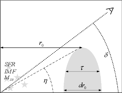
Figure 1: Schematic overview of the “physical” environment created in the simulations. In the center star formation is going on, which irradiates the dusty surroundings (here represented as a toroidal shape). This dust then re-radiates its given energy in the IR regime. Also the parameter space is shown. In the starburst, the total stellar mass ${\rm M_{SB}}$, the star formation rate (SFR) and the IMF-slope $\alpha$ are varied. In the dust the geometry is varied by changing the closing angle $\eta$. Also the dust column density (expressed as the optical depth $\tau$) is varied. A last variable is the observational inclination $\delta$. Also some parameters are shown, which initially were not varied: the radius $r_{0}$ and the radial scale size $dr_{0}$. More information on the parameter space can be found in Sect. 3.

Since both options are observationally supported, it is natural to think that there might be an evolutionary relation between the two. Several authors have suggested such schemes. In 1988, Baan explained the evolution of the FIR properties of active nuclei with a model which incorporated both a relatively rapid decreasing thermal SB component and a slower evolving non-thermal component.

Recently, more papers were published suggesting evolutionary schemes which incorporate both SB and AGN. Kawakatu et al. (2006) presented a sample of ULIRGs with type I Seyfert nuclei and showed with both observations and modeling that this type of galaxies can be powered by both a SB and a black hole (BH) with super-Eddington accretion. They suggest a scheme in which SB-powered ULIRGs and QSOs are two stages in the evolution of the host galaxy. The host will start as a SB-driven ULIRG, with only a small BH. Over time, the SB fades and the BH will grow into a super massive BH (SMBH), which will dominate the energy output of the host. By that time the host has become a QSO. Similar arguments are made by Hopkins et al. (2006) and Ho (2005). On the other hand, King (2005), Silk (2005) and Ho (2005) present schemes where the outflow of a super-Eddington accreting SMBH drives into the surrounding ISM, creating bubbles in which the gas cools and stars are formed. It is clear that detailed modeling is necessary to determine the evolution of ULIRGs and their engine(s).

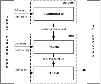
Figure 2: This flowchart shows the computational setup of the simulation. First the starburst properties are calculated using STARBURST99 (Sect. 2.1) and the results of these calculations are used as input for the dust calculations, which are performed by RADMC and RADICAL (Sects. 2.2 and 2.3).

In this paper, we focus on massive star formation as a central engine. In SB-powered ULIRGs, that are at sufficiently low redshift for their internal structure to be resolved, the great majority of the IR emission is found to originate from sub-kpc dusty regions within merging systems of galaxies (e.g. Downes & Solomon 1998). These dusty SB galaxies are an important class of objects. About 25% of the high-mass star formation within 10 Mpc distance from us occurs in just four SB galaxies (M82, NGC253, M83, NGC4945; Heckman 1998). Even though these galaxies create vast amounts of stars, the time scale of this formation is short. Near-IR imaging spectroscopy in M82, IC342, and NGC253 indicates that in the evolution of these galaxies there are several episodes of star formation activity, with timescales of around $10^{7}$ to $10^{8}$ years (Genzel & Cesarsky 2000). The relatively low efficiency of the energy production of stars ($E\sim 10^{-3}{\rm M}_{\star}{\rm c}^{2}$) and the large energy output (up to $\sim 10^{61}$ ergs for an ultra-luminous starburst like Arp220) yield a production $10^{8}$ to $10^{10}$ M_☉  of stars per burst. Combined with the short timescales, this leads to star formation rates (SFRs) ranging from 10 up to 1000 M_☉ per year (Heckman 1998). Numerical simulations confirm this picture. Jonsson et al. (2006) show that during a typical merger event, there are several short periods of star formation at a very high rate.

The goal of this paper is to present a model for these dust-enshrouded star formation regions and to study and explain the behavior of the broad band IR continuum properties of starburst ULIRGs during their evolution. The model consists of a number of existing codes, which are combined into one.

In future work, we will also investigate the spectral features in the IR regime, which will provide more diagnostics to determine the source of the activity in ULIRGs (e.g. Hollenbach & Tielens 1999; Genzel & Cesarsky 2000; Spoon 2003). We also intend to extend the model with a molecular environment, in order to further constrain the physical parameters of the cores of active galaxies (Meijerink & Spaans 2005). We will also investigate the similarities and differences between SB dominated and AGN dominated ULIRGs and will investigate the possibility of an evolutionary connection between the two.

The structure of this paper is as follows: in Sect. 2 the model is discussed. The parameter space and the simulations are presented in Sect. 3 and the results of these simulations in Sect. 4. In the last section the results are discussed and suggestions for future work are made.

2 The model

The “physical” setup of our model is shown in Fig. 1. A star formation region is placed in the center of our model, surrounded by a dusty environment, which is responsible for the re-emission of the stellar UV photons in the IR. The same scheme can be seen in Fig. 2, which shows the computational setup of the model. The first step in the simulations is the calculation of the spectral energy distribution (SED) of the star formation region using STARBURST99. The surrounding dust is modeled using RADMC and RADICAL, which use the stellar SED to calculate the dust temperature and the emergent IR radiation. The used codes will be briefly discussed and the interested reader is referred to the listed references for further details.

2.1 STARBURST99

As mentioned above, the stellar properties of the starburst are calculated using STARBURST99 (hereafter SB99), which is a set of stellar models, optimized to reproduce properties of galaxies with active star formation and their evolution through time. In this paper only a brief summary of the model is given. More information on the data produced by SB99 can be found in Leitherer et al. (1999). Detailed information on the computational techniques can be found in Leitherer et al. (1992) and Leitherer & Heckman (1995).

The calculations can roughly be divided into three stages. First an ensemble of stars is formed according to the available gas mass and the initial mass function (IMF), either in one instantaneous burst (i.e., the duration of the burst is short compared to the stellar life time) or continuous with a constant star formation rate (SFR). Because these two cases represent the extremes of star formation, realistic scenarios will lie somewhere in between (Leitherer & Heckman 1995; Leitherer et al. 1992).

After creating the stellar population, evolutionary models are used to calculate the time dependency of the stellar properties, such as stellar mass, luminosity, spectra, effective temperature, and chemical composition.

In the last stage of the calculation the integrated properties of the star formation region are computed by determining the stellar number densities, assigning all properties to these stars and integrating over the entire population (Leitherer & Heckman 1995).

2.2 RADMC

The output SEDs of the SB99 calculations are used to irradiate the dusty environment. In order to do this the SB99 spectrum must be re-binned to the number of channels the dust simulation codes can handle. The re-binning of the SB99 output is performed in such a way that both the UV/optical part of the spectra (which provides the energy for the dust heating) and the IR regime (which is the part of the spectrum of interest) are well covered. Since the SB99 output SED ranges from 100Å (extreme UV) up to wavelengths around $10^{6}$Å (100 $\mu$m; FIR) and the number of channels is limited, the resolution of the re-binned SED is low. Therefore, the re-binning is performed in such a way that the IR part of the SED has a somewhat higher resolution, so that the 10$\mu$m, 20$\mu$m, 60$\mu$m and 100$\mu$m bands are included, in order to compare the resulting IR data with IRAS observations. Because, in this work, we are focusing on defining a physical framework for an evolutionary model and not on the details, and also taking the low spectral resolution and the simple dust model into account, we did not compare our results with more recent ISO or Spitzer data. Readers who are interested in more detailed models which are not taking evolution into account are refered to, for instance, Efstathiou & Rowan-Robinson (1995), van Bemmel & Dullemond (2003), Fritz et al. (2006) and references there in.

The physical dust environment is simulated by creating a dust density grid with a central cavity, which is the region surrounding the central SB where the dust is destroyed and/or blown away by the star formation activity. Since we also want to explore the influence of the dust geometry on the emergent SEDs in our simulations, a 3D grid is needed. This, however, would lead to long calculation times. In order to limit this problem, the grid is chosen to be axisymmetric. This way the grid is reduced to two dimensions again, but still allows for various astrophysically interesting dust distributions, like shells, tori and disks.

RADMC is a 2-D Monte-Carlo radiative transfer code for axisymmetric circumstellar disks and envelopes. It is based on the method of Bjorkman & Wood (2001), but with several modifications to produce smoother results with fewer photon packages.

Table 1: This table lists the parameters used for the simulations. The top half of the table shows the default simulation and the simulations done in the second stage. In this stage the large scale parameters were varied. The bottom half shows the simulation from the third stage, where the influence of the second dust component was investigated. All simulations were calculated for inclinations 0, 30, 60 and 90 degrees. The names chosen for the simulations represent the parameter investigated in that simulation. Parameters not listed for a simulation were not used in that simulation.

name	${\rm M_{SB}}$	$\alpha$	$\tau$	$\eta$	SFR	$r_{0}$	$r_{1}$	$dr_{1}$	$\eta_{1}$	$\tau_{2}$	dust
	$\log{}{\rm M}_{\odot}$	$M^{-\alpha}$		0-1	M☉/yr	pc	pc	pc	0-1
DEFAULT	9	2.35	10	0.3							grey torus
LOWMASS	8	2.35	10	0.3							grey torus
HIGHMASS	10	2.35	10	0.3							grey torus
LOWALPHA	9	1.3	10	0.3							grey torus
HIGHALPHA	9	3.3	10	0.3							grey torus
LOWTAU	9	2.35	1	0.3							grey torus
HIGHTAU	9	2.35	100	0.3							grey torus
COVERED1	9	2.35	10	0.5							grey torus
COVERED2	9	2.35	10	0.7							grey torus
CONTINUOUS		2.35	10	0.3	100						grey torus
30pcTORUS	9	2.35	10	0.3		30					grey torus
50pcTORUS	9	2.35	10	0.3		50					grey torus
10pcSHELL	9	2.35	10	0.3			10	10	1	$\tau+\tau_{2}$ = 10	grey torus and grey stellar
10*10pcSHELL	9	2.35	10	0.3			10	10	1	$\tau+10*\tau_{2}$ = 10	grey torus and grey stellar
FINAL	9	2.35	10	0.3			10	10	1	0.1	grey torus and non-grey stellar

The method introduced by Bjorkman & Wood (2001) is to divide the luminosity of the radiation source (in this case the re-binned output spectrum of SB99) into equal-energy, monochromatic “photon packets” that are emitted stochastically by the source. The packets are then traced to random interaction locations on the dust grid, determined by the optical properties and density distribution of the dust. In every iteration step, the number of packets absorbed in each of the grid cells is recorded and the total amount of injected energy is used to calculate the new temperature of that cell. In order to ensure energy conservation and radiative equilibrium, the absorbed energy must be re-emitted immediately. The frequencies of the new packets are determined by the new grid cell temperature. Local thermal equilibrium (LTE) is assumed, so the amount of emitted energy equals the absorbed energy.

Because all the injected packets eventually escape and so does all the injected energy, the total energy is automatically conserved. Another advantage of this approach is that the simulation does not have some sort of convergence criterion to meet, so that the only source of error in the calculation is the statistical error inherent to Monte Carlo simulations.

One problem with the Bjorkman & Wood method is that it produces very noisy temperature profiles in regions of low optical depth, and requires a large number of photons ($N\sim 10^{7}$) for a smooth SED. These disadvantages have been solved in RADMC by treating absorption partly as a continuous process (see Lucy 1999 for more information), and using the resulting smooth temperature profiles with a separate ray-tracing code (RADICAL) to produce images and SEDs. These images and SEDs have a low noise level even for relatively few photon packages ($N\sim 10^{5}$). This improved Bjorkman & Wood method works well at all optical depths, but may become slow in cases where the optical depth is very large ($\tau_{\nu}\sim$ 1000; see Pascucci et al. 2004); this situation is not reached in our simulations.

2.3 RADICAL

RADICAL produces the final spectra, by solving the radiative transfer equation on the entire grid, using the dust temperature and the SED of the central source to calculate the source function.

First an image is created by integrating the source function along rays through the medium. Each ray represents one pixel of the image. Spectra can be derived by making images at a range of frequencies, and integrating these over an artificial detector aperture.

Resolution problems may occur, since the source spans a large radial range. The central parts of the image are often much brighter than the rest, but cover a much smaller fraction of the image. The spectrum may therefore contain significant contributions of flux from both the central parts and the outer regions of the image. Unless the image resolves all spatial scales of the object, the spectra produced in such a way are unreliable. Therefore, rather than arranging the pixels over a rectangle, as in usual images, they are arranged in concentric rings. The radii of these rings are related to the radial grid points of the transfer calculation. To resolve the central source, some extra rings are added. Using these kind of images, all relevant scales are resolved, while using only a fairly limited number of pixels (Dullemond & Turolla 2000).

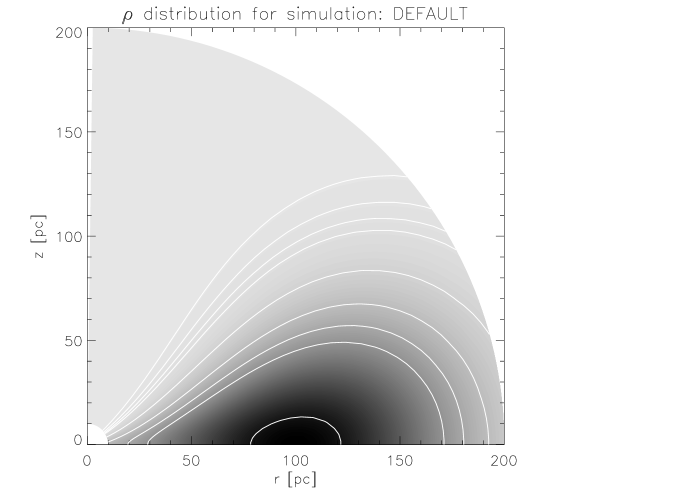
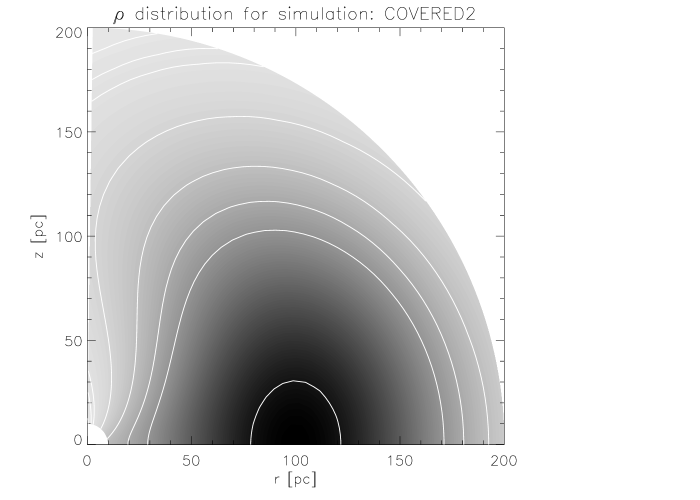
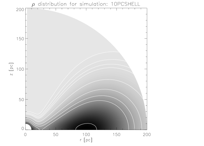
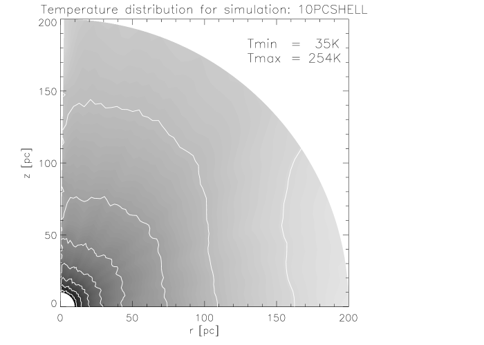
Figure 3: These figures show three examples of the dust and temperature distributions resulting from the simulations. The top panels show the dust density in grey scale, where dark colors indicate regions with high densities and light colors are low density regions. Also some contours are added to enhance the shape of the density profile. The bottom panels show the temperature distribution. In these panels, dark colors indicate high temperatures and light colors cooler regions. The minimum and maximum temperature is printed in the upper right corner of the panels. Contours are drawn from 50 to 250K in steps of 25K. The data in these plots was smoothed over 3 pixels to make the general temperature distribution more clear. The left panels show the default simulation, the middle ones a setup with $\eta=0.7$ and the right ones a default distribution with an extra 10 pc shell of grey dust.

3 The simulations

In this section, the simulation setup and the parameter space are discussed. As shown in Fig. 1, there are 6 parameters, which control the simulation: the combined mass of the stars in the starburst ${\rm M_{SB}}$, the star formation rate (SFR), the IMF slope $\alpha$, the closing angle of the dust distribution $\eta$, the dust column expressed in the edge-on V-band optical depth $\tau$ and the observation declination $\delta$.

This parameter space has been explored, starting with values chosen either from literature or at random. In order to verify the results of the simulations, a reference data set was made using IRAS data of starburst galaxies taken from the extended 12 micron galaxy sample (Rush et al. 1993) and the IRAS Bright Galaxy Sample (Condon et al. 1991).

From the simulations a default set is chosen, which fits the data best. This set will be referred to as DEFAULT. This set was chosen as the starting point for a more systematic sweep of the parameter space. Each parameter was both increased and decreased with respect to the default value. Exceptions are the closing angle $\eta$, the inclination $\delta$ and the SFR. Both permutations of $\eta$ are higher than the default value. The inclination was varied in all simulations: each setup was calculated for $\delta$ = 0, 30, 60 and 90 degrees. The SFR was only used in few simulation. In the other simulations, all stars are formed instantaneous. The entire parameter space is listed in Table 1.

3.1 STARBURST parameters

The SB in the center of the simulation has a large number of parameters. Only three are chosen as variables, in order to reduce the amount of data and to avoid unnecessary redundancy. These parameters are also expected to have the largest influence on the final results. The fixed parameters are listed in Table 2.

The variable parameters are the total mass of the stars involved in the starburst (${\rm M_{SB}}$), the star formation rate (SFR) and the IMF slope ($\alpha$). These were chosen because the large luminosities of ULIRGs can be explained by either a high total burst mass, a high SFR or a lower IMF slope exponent. Adding more stars or increasing the SFR will scale the entire spectrum, whereas decreasing the IMF slope increases the relative number of heavy stars, leading to more UV radiation and therefore more heating flux (as suggested in Heckman 1998).

Table 2: This table lists the parameters which determine the simulations, but were not varied. The upper part of the table lists the SB99 parameters, the lower part the RADMC parameters.

name	value
IMF upper mass limit	100	M☉
IMF lower mass limit	1	M☉
supernova cut-off mass	8	M☉
black hole cut-off mass	120	M☉
initial time	0.01	Myr
time step	0.1	Myr
end time	20	Myr
wind model	theoretical
atmosphere model	Pauldrach/Hillierb
metallicity of UV line spectrum	solar
$r_{0}$	100	pc
$dr_{0}$	50	pc

3.2 Dust setup

The dust distribution is made by creating a polar grid, with a density on each grid point. The shape is created by introducing a Gaussian distribution in both the $r$- and $\theta$-direction:

$$\rho\left(r,\theta\right)=\exp{\left[-\frac{1}{2}\left(\frac{\pi/2-\theta}{\eta}\right)^{2}-\frac{1}{2}\left(\frac{r-r_{0}}{dr_{0}}\right)^{2}\right]}\leavevmode\nobreak\ ,$$ (1)

where $\rho\left(r,\theta\right)$ is the dust density on each grid point, $r$ is the radial direction, $\theta$ the angular direction, $r_{0}$ the radius of the dust geometry, $dr_{0}$ the radial scale size and $\eta$ the closing angle. This density distribution is then fixed by scaling the edge-on optical depth (obtained by integration along the line of sight) to the desired V-band optical depth $\tau$. Three examples of resulting density distributions are plotted in Fig. 3. From this two-dimensional grid, a three-dimensional grid is made by first mirroring the grid on the $r$-axis and then rotating this semi-circle around the z-axis.

Two dust components are created: a large scale component distributed in a thick disk/torus (here after called torus dust) and a small scale shell (called stellar dust). The torus dust distribution is created by using an $r_{0}$ of 100 pc and closing angles ($\eta$) between 0.3 and 0.7. The stellar dust distribution is made by taking an $r_{0}$ of 10 pc and an $\eta$ of 1, making it a closed shell.

Besides the density and geometry, also the optical parameters of the dust must be specified. The dust used in the simulations has a grain size distribution $n(a)\propto a^{-3.5}$ (Mathis et al. 1977). The torus dust is assumed to be optically grey, i.e., radiation of all frequencies is absorbed in the same way and re-radiated using a black body profile. The stellar dust is much closer to the SB and will be hotter. In order to model the expected richer spectral properties of this component, the stellar dust is assumed to be composed of graphite, silicates and amorphous carbon (e.g. Draine & Lee 1984).

4 Results

The code produces four broadband IR fluxes as a function of time. These fluxes are used to calculate the IR luminosity (${\rm L_{IR}}$) following the definitions given in Sanders & Mirabel (1996) and Kim & Sanders (1998).

The simulations were carried out in three stages. First a default simulation was made. In the second stage the large scale parameters, like the starburst and the torus dust, are explored, which influence the long wavelength radiation. The last stage focuses on the stellar dust, which affects the short wavelength emission.

4.1 Stage 1 - The default simulation

The results of the default simulation from the first stage are plotted in Fig. 5. The first 4 panels show the results for the four IRAS bands. As can be seen the simulation results match the reference set quite well. Only the shortest wavelength at 10$\mu$m seems to be a poor fit. This is due to the fact that in this stage we have not included the stellar dust yet (see Sect. 4.3 for the stellar dust). This dust component will radiate mostly at short wavelengths.

The calculated ${\rm L_{IR}}$, which is plotted in the fifth panel, also covers the range observed in galaxies. At the peak of its activity the luminosity of the starburst exceeds $10^{12}$ L_☉, making it a ULIRG. It remains that luminous for about 3 Myr, after which it slowly dims and eventually reaches the LIRG regime.

In the last three panels of Fig. 5, three IR colors (10$\mu$m/100$\mu$m, 20$\mu$m/100$\mu$m and 60$\mu$m/100$\mu$m) are plotted versus the IR luminosity. These color-luminosity diagrams (CLDs) show results similar to the IRAS fluxes. The 20$\mu$m/100$\mu$m and 60$\mu$m/100$\mu$m results match the observations, whereas the 10$\mu$m/100$\mu$m is a poor fit, due to the absence of the stellar dust.

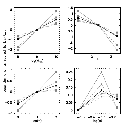
Figure 4: These panels give an overview of the simulation results. The four IRAS bands (in grey: 10$\mu$m solid, 20$\mu$m dashed, 60$\mu$m dash-dotted and 100$\mu$m dotted) and the IR luminosity (black solid) are shown as a function of the various parameters (top-left: ${\rm M_{SB}}$, top-right: $\alpha$, bottom-left: $\tau$, bottom-right: $\eta$). The points represent the values at 2Myr, which is the time where the luminosity of the system is at its maximum. All data were scaled to the results of DEFAULT, in order to make an easy comparison. Note that the results for the SFR are not included in these plots. Also the observational inclination $\delta$ was not included: the data are taken from the face-on results.

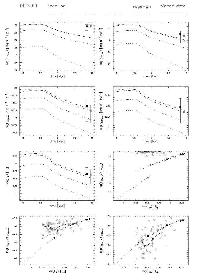
Figure 5: These panels show the infrared results of the simulation DEFAULT. The top 4 panels show the 10, 20, 60 and 100$\mu$m flux as a function of time. The fifth panel shows the calculated infrared luminosity (${\rm L_{IR}}$) through time. The last three panels give a more observational interpretation of the data. In these panels three IR colors (10$\mu$m/100$\mu$m, 20$\mu$m/100$\mu$m and 60$\mu$m/100$\mu$m) are plotted versus the IR luminosity. To indicate the evolution direction, the start of the track is marked with a star. All axes are logarithmic except the time axes. The observational inclinations are indicated by the line style: from face-on in solid, through dashed and dash-dotted to edge-on indicated with dotted lines. The two reference data sets are added with markers. In the first 5 panels, the error markers represent the mean of these data sets and a 1 $\sigma$ deviation. The grey marker is data from the 12 micron galaxy sample (Rush et al. 1993) and the black one from the IRAS Bright Galaxy Sample (Condon et al. 1991). In the last three panels, the data from the 12 micron galaxy sample is indicated by circles and the data from the IRAS Bright Galaxy Sample by squares. The black dots connected by a solid line show the reference data binned per 10 points.

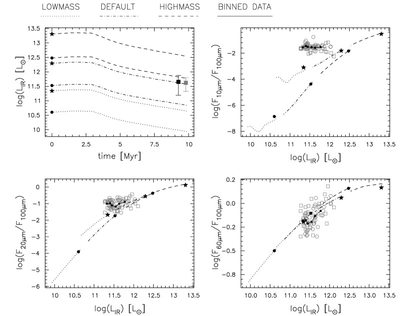
Figure 6: These panels show the influence of the starburst mass (${\rm M_{SB}}$) in the infrared results. The two deviations are compared to the default value. The simulation results for the lower deviation are indicated by dotted lines, the higher deviation by dashed lines and the default set is drawn in dash-dotted lines. The face-on observations are marked with a star, the edge-on results with a circle. These marks also indicate the start of the evolutionary track, to indicate the evolution direction. The panels are the same as the bottom four panels of Fig. 5: the first panel shows the IR luminosity as function of time and the other three panels show three IR colors (10$\mu$m/100$\mu$m, 20$\mu$m/100$\mu$m and 60$\mu$m/100$\mu$m) versus the IR luminosity. As in Fig. 5 the two reference data sets are added with markers. In the first panel, the error markers represent the mean of these data sets and a 1 $\sigma$ deviation. The grey marker indicates data from the 12 micron galaxy sample (Rush et al. 1993) and the black one from the IRAS Bright Galaxy Sample (Condon et al. 1991). In the last three panels, the data from the 12 micron galaxy sample is indicated by circles and the data from the IRAS Bright Galaxy Sample by squares. The black dots connected by a solid line show the reference data binned per 10 points.

The default results exhibit a strong dependence on inclination. The difference between edge-on and face-on ranges from a factor of 3.2 at 100$\mu$m up to 1000 at 10$\mu$m, with an average factor of 5.6 in the ${\rm L_{IR}}$. This large separation at short wavelengths is caused by the dust distribution. As can be seen in Fig. 3, the resulting temperature distribution is not spherical. Along the edge-on line of sight the optical depth is 10, whereas along the face-on line of sight the star formation region is almost “naked”. This causes the areas with lower temperature to become more flattened, compared to the inner, high temperature areas. When this temperature distribution is viewed edge-on, the cooler isothermal surfaces are seen at their maximum surface area and when observed face-on, their surface areas decrease rapidly. On the other hand, the inner high temperature regions are roughly spherical and will therefore look the same from all directions. The overall face-on spectrum will thus have a larger contribution at short IR wavelengths, as compared to the edge-on spectrum. This is also illustrated in the lower right panel of figure 3, which shows the temperature distribution of simulation COVERED2, in which the cooler dust is more spherical and the inclination dependence of the 10$\mu$m flux is an order of magnitude smaller. Another effect of the dust distribution is that short wavelength radiation emitted in the center will encounter much more dust when it is traveling along the edge-on line of sight compared to face-on, making the chance of it getting scattered or re-processed much larger.

The effect of this inclination dependence can also be seen in the three CLDs in figure 5. At short wavelengths (10$\mu$m/100$\mu$m and 20$\mu$m/100$\mu$m) the face-on observations trace the data sets, whereas the edge-on results cover an entirely different range. This effect will be discussed in more detail, when the results of the other simulations are presented.

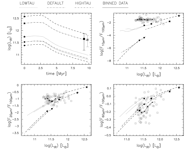
Figure 7: These panels show the influence of the dust optical depth ($\tau$) on the infrared results. The color coding is the same as in Fig. 6.

4.2 Stage 2 - Large scale parameters

In this section the parameters influencing the star formation and the torus dust are explored. Each parameter was varied twice, in most cases “in both directions” from the default values, in order to uncover systematic effects. The observational inclination will not be discussed, since the effects of the inclination have already been discussed above. The figures which show the most important effects have been included in this article. An overview of the results is shown in Fig. 4. The rest of the figures displaying all the results, including the four IRAS fluxes, of the individual simulations and comparisons between them are collected in Appendices A and B respectively.

4.2.1 Starburst mass

The effect of the starburst mass on the SB99 spectra is quite simple. Since this code works with a distribution of stars, integrated to a certain mass, the spectra will scale proportional to the total stellar mass. The influence on the dust is less straightforward, however. When the energy input provided by the starburst increases, the overall dust temperature will be higher and the flux at short wavelengths will increase faster relative to the long wavelengths. Also the IR luminosity is expected to increase with the stellar mass, since the energy input increases.

The simulations confirm these expectations. Figure 4, which gives an overview of the results of the simulations, clearly shows that the short wavelengths (grey solid and dashed) increase much faster than the long wavelengths (grey dash-dotted and dotted) and that ${\rm L_{IR}}$ (black) increases as the mass increases.

The color-luminosity plots in Fig. 6 seem to reveal less trivial information. Assuming all the other parameters are correct, a minimal SB mass of $10^{9}$ M_☉  is needed in order to create an IR luminosity higher than $10^{12}$ L_☉. Also all three simulations seem to lie on the same “track” in the CLDs, and starburst mass and age have the same effect on the results. In other words, a young, but relatively light starburst will, in IR colors, have the same appearance as a massive, older starburst.

4.2.2 IMF slope

When the IMF slope decreases, the number of massive stars in the starburst will increase. These high mass stars are the main source of UV radiation, and so the dust temperature will increase with a shallower IMF slope. This means that varying the IMF slope would yield results similar to increasing the starburst mass.

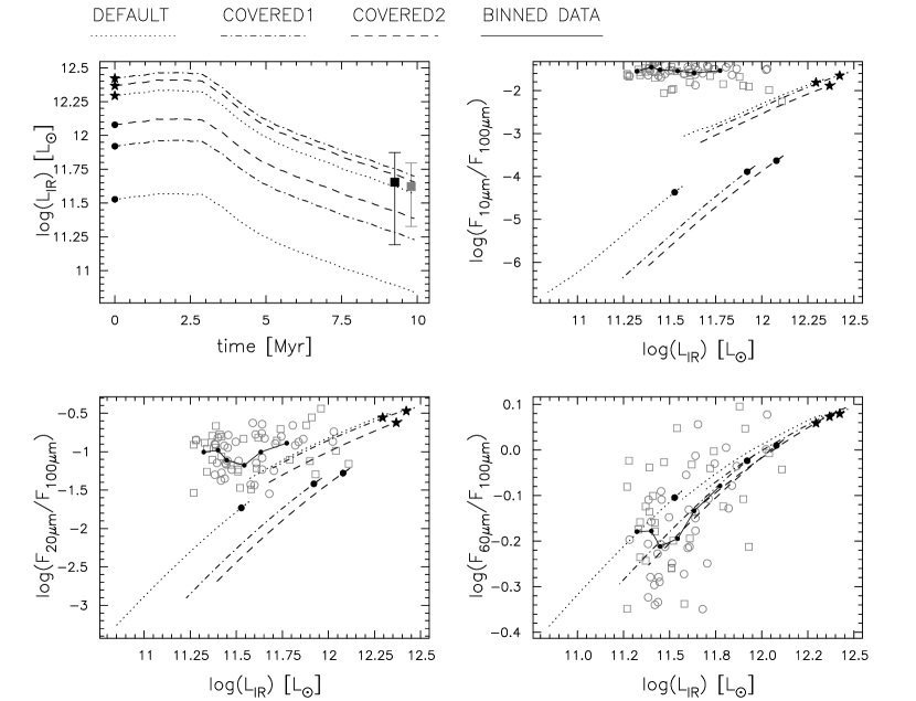
Figure 8: These panels show the influence of the closing angle ($\eta$) on the infrared results. The color coding is the same as in Fig. 6. Note: for this simulation both deviations are higher than the default value.

Figure 4 shows this is indeed the case. Note that at first sight the effect seems to be reversed, but the IMF is defined as $\Psi(M)\propto M^{-\alpha}$, and the axis is reversed. Interestingly, the effect is somewhat more complicated than for ${\rm M_{SB}}$. All fluxes scale proportionally to ${\rm M_{SB}}$, but the effect is stronger when going from high $\alpha$ to the default value, then when lowering it even further. This is caused by the fact that the number of OB stars does not increase linearly with $\alpha$.

Figure B.2 shows that although LOWALPHA starts with higher values for the IR luminosity and the colors, after about 10 Myr the low IMF case cannot be distinguished from the default simulation any more. This is due to the short life time of the high mass stars. Therefore, the same conclusion can be drawn for the IMF slope as for the starburst mass: the data either represent young starbursts with a normal IMF, or an older population of stars with a shallow IMF slope.

4.2.3 Dust column density

Several effects have been identified when changing the total amount of dust for a given energy input.

First, when the dust column is lower, the dust will be heated more evenly, since the radiation can travel through the dust easier. This will result in a smaller temperature gradient, with a higher minimum temperature. The spectrum will become flatter, and have less contribution from 10$\mu$m and 20$\mu$m. Conversely, large dust columns lead to larger dust temperature gradients and steeper spectra. This effect is shown in Figure 4, where the variation of $\tau$ has effects similar to ${\rm M_{SB}}$ and $\alpha$.

Second, due to the larger temperature gradient, the inclination dependence increases for larger $\tau$. In Figure 7, this effect can be seen in the first panel, where the edge-on and face-on results are almost the same for LOWTAU, whereas the results for HIGHTAU differ by up to an order of magnitude.

A third effect is the increase in the total IR luminosity ${\rm L_{IR}}$, simply because there is more radiating dust and therefore more UV photons can be converted into IR.

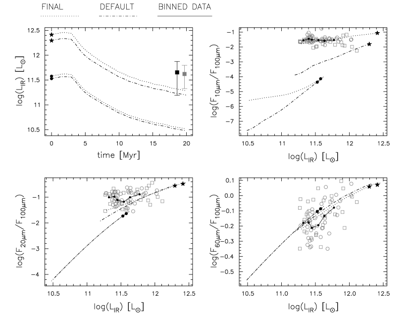
Figure 9: These panels show the influence of adding the stellar dust component on the infrared results. The color coding is the same as in Fig. 6. Note: to show that the whole reference set is traced in the CLDs, 20 Myr is shown instead of 10.

All these effects can be found in the color-luminosity diagrams. When going from LOWTAU to DEFAULT especially ${\rm L_{IR}}$ increases, resulting in a shift to the right. But when $\tau$ increases even more, the color changes rapidly, and the track moves to the upper right corner of the plot. Again, due to the inclination effects, the edge-on results do not match the reference sets. The edge-on results of LOWTAU are better, because they suffer less from inclination effects, but they give worse fits than the face-on DEFAULT results.

Like in the previous simulations, there is a degeneracy between $\tau$ and time. Young starbursts surrounded by moderate column density dust have the same IR properties as older, more enshrouded starbursts.

4.2.4 Closing angle

The effect of the closing angle is not as profound as that of the other parameters. The only major effect is that the inclination dependence effects are reduced, which is caused by a smaller density gradient in the $\theta$ direction (also see Fig. 3). The extreme case would be a simulation with $\eta=1$, which is a shell of dust with no inclination dependence at all.

Although the inclination effects are less in simulations with a higher closing angle, the edge-on tracks in the color-luminosity tracks of Fig. 8 still do not fit the reference data.

The shape of the spectrum also changes when the closing angle changes, but this is due to the fact that the total dust column changes, since the edge-on optical depth is kept constant.

4.2.5 Star formation rate

So far, all simulations were made under the assumption that the stars were formed instantaneously, or, in other words, on a timescale much shorter than the evolutionary timescale of the stars ($\lesssim$ 1 Myr). This is based on the assumption that there is a rapid build-up of gas in the starburst environment, which at some point becomes critically dense and “ignites”. It also assumes that the stellar winds and supernovae do not provide strong feedback, so that all gas can be converted into stars on a short time scale. However, the assumption that the starburst environment is less violent and more like normal star formation regions, with a steady inflow of gas, is also valid and must be explored as well.

In order to address this issue, simulations were done with continuous star formation scenarios with different SFRs and durations as presented in Figs. A.10, B.5 and B.10. It was found that a SFR of several tens of M_☉ yr^-1 is required to reproduce the fluxes found in observational data. Simulations with a duration of 100 Myr show that after about 10-20 Myr there is no further evolution in the IR fluxes and colors. However, our data cannot exclude longer burst durations, but there are considerations that would make such scenarios unlikely. First of all, long periods of star formation at high rates would require vast amounts of gas. Secondly, these high star formation rates also produce a lot of stellar feedback (stellar winds, SNe) that makes it increasingly difficult to supply gas to form new stars.

Because of these reasons, we consider the case of a high SFR and a short duration (100 M_☉ yr^-1 and 10 Myr, leading to the formation of $10^{9}$ M_☉  of stars, and making it comparable to the other simulations). The results of this simulation are compared to DEFAULT in Fig. B.5. This figure shows some remarkable differences between the two situations. Whereas the instantaneous burst starts at a maximum and decays rapidly after about 3 Myr, the continuous case starts at much lower values and takes quite some time to rise. After about 5 Myr the two scenarios cross and the continuous case starts to dominate. After about 10 Myr it reaches its maximum, but it does not decay, since stars keep forming at a constant rate.

The significant difference between the continuous and the instantaneous star formation is that objects with instantaneous star formation are only luminous enough in the first 5 to 10 Myr, which decreases their detection rate. The continuous starbursts remain luminous as long as there is inflow of gas to feed the star formation.

4.3 Stage 3 - Stellar dust

The torus dust alone is not able to explain all the IR continuum properties and therefore in the second set of simulations addresses the properties of the stellar dust component. The lack of emission at short wavelengths can have two reasons. A very simple explanation is that the geometry we are currently using does not provide enough hot dust and more dust must be added in the center of the dust distribution. Another possibility is that the optical properties of the large-scale dust are inappropriate and that the stellar dust modelling requires more realistic optical properties.

4.3.1 Smaller radius

One of the ways to create more hot dust is to decrease the size of the total dust distribution. This way all the dust will be closer to the central source and therefore the overall temperature will be higher. In order to investigate this possibility, two simulations were carried out, with $r_{0}=50$ pc and $r_{0}=30$ pc. The rest of the parameters were the same as for DEFAULT. As can be seen in Fig. B.6, decreasing $r_{0}$ does improve the short wavelength results. However, it also affects the longer wavelengths and although the fit in the 10$\mu$m/100$\mu$m CLD is better, the slope is not correct. A positive effect is that is introduces scatter in the vertical direction of the CLD, which could not be explained well by the previous simulations. Overall one can conclude that although changing the radius of the dust geometry does improve the results, it does not provide the hot dust contribution that we are looking for.

4.3.2 Grey stellar dust

Another possible solution is to add additional stellar dust close to the starburst. Maybe our assumption that the dust close to the central region is completely destroyed or blown away is not correct. Therefore, we introduce an extra (Gaussian) dust shell with a scale size of 10 pc (see also Fig. 3). Two simulations are performed, one where the total column of both the stellar and the torus dust is scaled to an optical depth of 10 and one where the dust density of the stellar component is first multiplied by a factor of 10 and then the total column is scaled to an optical depth of 10. Again, the rest of the parameters are the same as for DEFAULT. Fig. B.7 shows that introducing this second component does increase the 10$\mu$m flux, without affecting the 60$\mu$m and 100$\mu$m fluxes. However, the 20$\mu$m flux is still influenced, and the 10$\mu$m flux cannot be increased further, without compromising the 20 $\mu$m results. These simulations also introduce scatter perpendicular to the evolutionary tracks.

Both attempts to solve the 10$\mu$m problem by introducing extra hot dust, do not provide the results that are desired. This suggests that the optical properties of the dust must be modified.

4.3.3 Non-grey stellar dust

Since the stellar dust component must have non-grey optical properties, it it will be composed from graphite, silicates and amorphous carbon (as described in Draine & Lee 1984). In these computations, the SB99 output spectrum is first processed by the non-grey stellar dust and the emergent radiation is used to irradiate the (grey) torus dust distribution.

As can be seen in Fig. 9 (see also Fig. A.11 and Fig. B.8 for the full results and Fig. 10 and Fig. A.12 for SEDs), the addition of non-grey stellar dust finally produces the right amount of 10$\mu$m radiation, without influencing the flux at longer wavelengths. In addition, although this second dust component has a large influence on the 10$\mu$m radiation, only a very low optical depth is needed, which corresponds to a small amount of dust (see Fig. B.9). The final results are created using an V-band optical depth for the second component ($\tau_{2}$) of only 0.1. In terms of mass this means that the amount of dust in the second component is about 0.1% of the total dust mass. Observationally, similar values are found. For instance, Klaas et al. (1997) found that in order to properly fit the SEDs of Arp 244, NGC 6240, and Arp 220, they need to add about 0.1% of hot dust to the bulk of the (colder) dust.

Physically, the stellar dust component most likely represents the left-overs of the dust, which was shocked by stellar ejecta and blown away by the stellar radiation. This dust is much closer to the stars than the torus dust, is hotter and experiences disruptive events like sputtering and shattering. A simple grey dust model does not give the right results, since for these smaller grain sizes the wavelength dependence of the absorption cross section is important (e.g. Spoon 2003; Peeters et al. 2004). The torus dust is the ring or shell of dust surrounding the starburst nucleus. It has higher column densities, larger grain sizes and is further away, giving rise to lower dust temperatures. Therefore, the grey approximation is valid for this dust component.

Figure 10: These panels show the evolution of the emergent spectrum of our final simulation. The top panel shows four spectra as a function of time ranging from t=0 (black) to t=15Myr (light grey) in steps of 5Myr. The bottom panel shows the same spectra, but this time divided by the spectrum of t=0. All spectra were taken from the face-on results.

5 Conclusions

Our simulation model is able to reproduce the IR continuum properties of starburst galaxies, by using two dust components: a large scale component containing the bulk of the mass and a less massive component close to the starburst. The long wavelength radiation is influenced by macro-physics like the star formation activity and the large scale dust distribution. The short wavelength emission at 10 $\mu$m comes from hot dust and is influenced by the stellar dust and micro-physics like the optical properties and optical depth of the dust.

Not all parameters have a profound effect on the results. The stellar dust optical depth ($\tau_{2}$) and the parameters controlling the star formation (the total stellar mass ${\rm M_{SB}}$ and the IMF slope $\alpha$) have a large effect on the final results, whereas the influence of the large scale dust geometry ($\tau$ and $\eta$) on the final IR properties is smaller.

Star formation region
Because of their large influence on the results, the star formation parameters could be determined well. Increasing the stellar mass (${\rm M_{SB}}$) has two effects. First of all, the shape of the spectrum changes, the short wavelength fluxes increase as compared to the long wavelengths. A second effect is an increase in ${\rm L_{IR}}$, which changes a factor of 10 when changing the mass by a factor of 10. The effects of varying the IMF slope ($\alpha$) are similar to those of the stellar mass, but are less pronounced when decreasing $\alpha$ than when increasing it. Making the IMF slope more shallow increases the luminosity by a factor of 4.0, whereas steepening the slope decreases the luminosity by a factor of 7.9. There is a degeneracy between ${\rm M_{SB}}$ and $\alpha$. A less massive starburst with a shallower IMF will produce roughly the same amount of OB stars as a more massive starburst with a steeper IMF and therefore the same amount of massive stars and therefore the same irradiating UV flux. Assuming the stars are formed according to a Salpeter IMF ($\Psi(M)\propto M^{-2.35}$), the star formation region should produce $10^{9}$ M_☉  of stars (either in one instantaneous burst or in a continuous process) in order to produce enough IR radiation.

Stellar dust
For the stellar dust component, the grey approximation of the optical dust properties is not valid. A more realistic dust model, including graphite, silicates and amorphous carbon, is necessary to produce the right results. In addition, the V-band optical depth ($\tau_{2}$) is found to be an important factor. Using a $\tau_{2}$ of 10 (or 1) overproduces the amount of 10$\mu$m radiation by almost a factor of 4 (or 2.5). We require an optical depth of 0.1 to get values that agree with observations.

Torus dust
The influence of the large scale dust geometry on the final IR properties was far less and therefore these parameters could not be determined to great precision. Increasing the dust column density ($\tau$) has two effects. Like for ${\rm M_{SB}}$, the short wavelengths are enhanced compared to the long wavelengths and the IR luminosity increases. These effects are, however, much smaller: the luminosity changes by a factor of 2.0 when going from $\tau$=1 to 10 and by a factor of 3.2 when increasing it further to 100. A second effect is that the inclination dependence increases with increasing optical depth. The difference in the edge-on and face-on values of ${\rm L_{IR}}$ changes by a factor of 1.6 for $\tau=1$ to a factor of 16 for $\tau=100$. The best fit to the data was obtained with $\tau=10$, but the other simulations were also reasonable. The closing angle did not seem to have an optimum value at all. Varying it only affects the inclination dependence of the results. The variation of ${\rm L_{IR}}$ for a flat disk-like structure ($\eta=0.3$) is about a factor of 6.3, compared to a factor of 2.0 for a more shell-like dust geometry with a closing angle of 0.7. Even though the inclination effects are reduced for higher values, the edge-on results still do not match the data.

Considering the values determined for the parameters investigated, it seems that, although observationally starburst galaxies appear to have a very violent nature, the star formation environment does not need to be as “exotic” as one might expect. The only exceptional parameter needed to explain the high IR output of starburst galaxies is the large amount of massive stars (high ${\rm M_{SB}}$ or SFR), but there is no need for an adjusted IMF to increase the number of heavy stars. The torus dust surrounding the stars is no exception to this trend. Both the size (100 pc) and the V-band optical depth of the torus dust are moderate (10, comparable to values found for photon dominated regions). Furthermore, most of the dust has a low temperature ($\sim 75$K at 100pc from the center), while only a very small amount of hot dust ($\sim 400$K at 10pc) is needed.

In all simulations, including the final ones, the data were only fit well by the face-on evolutionary tracks. All the completely edge-on results were a poor fit. This effect is stronger in the short wavelength results than in the long wavelength result. This indicates that inclination dependence is mostly caused by the obscuration of the hot dust in the center by the outer dust distribution. This can have two implications. On the one hand, it could be that the inclination dependence resulting from our model is too large, and that extra parameters are needed to address this problem. A likely parameter is the clumpiness of the dust. A clumpy medium with the same average density (i.e. the same mass) would have a lower apparent optical depth then a smooth medium (e.g. Natta & Panagia 1984; Conway et al. 2005), which makes it easier for the short wavelength radiation to travel in the edge-on direction. On the other hand, if the predictions of our model are correct, the implication is that there is a significant number of starburst ULIRGs, which are currently not classified as such based on their IRAS colors.

A specific shortcoming of our models is that, although the IR properties are well explained, almost all parameters move the evolutionary tracks more or less along the same line and in the direction of the evolution. The result is that not all parameters of the physical environment in a given starburst galaxy can be uniquely inferred from observations, using this model. The UV input can be inferred from the total IR output, but this does not constrain the IMF or the SFR. Similarly, the optical properties of the dust can be determined, but the geometry is hard to infer. To address these problems, more information than just the IR continuum is needed and therefore we intend to extend the current model. First of all, the IR part of the code will be modified to include specific spectral characteristics (e.g. PAHs and high ionization lines). Also the molecular environment that surrounds the current dust region will be added to the model. The chemistry of such a region will give a better handle on the radiation field, as well as the densities and temperatures of the gas (e.g. Hollenbach & Tielens 1999; Meijerink & Spaans 2005; Aalto et al. 2002; Usero et al. 2004; Gao & Solomon 2004; Ott et al. 2005; Graciá-Carpio et al. 2006; Baan et al. 2006) . Also other wavelengths will be studied, since optical and UV data will give more information about the star forming region, whereas (sub)millimeter and radio observations will reveal more about the outer dust regions and the molecular environment.